3.1. Material A
From the ratio between the amount of CO
2 produced at time t (raw data) and the theoretical one (corresponding to full biodegradation of the dry material mass loaded initially, m°, based on its carbon content, as Equation (1)), we calculated the fraction of CO
2 produced, which represents the degree of advancement (
X) of the biodegradation reaction. The amount of residual polymer m(t) at time t was calculated from the formula
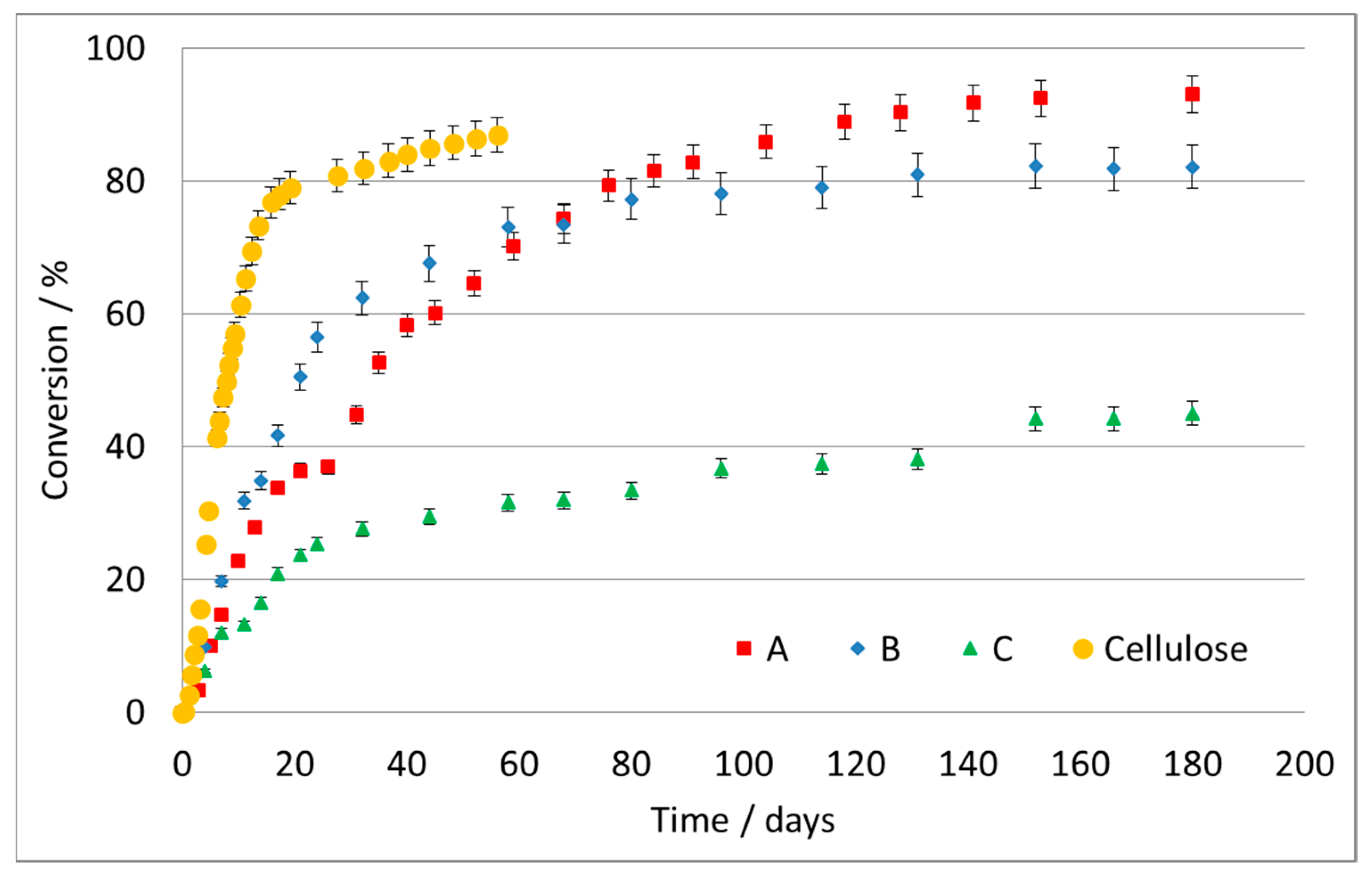
Figure 1 reports the conversion, as a percentage, as a function of time for the three tested samples of different materials and the cellulose used as reference.
The cellulose biodegradation data revealed very fast degradation in few days in the compost material used, assessing the validity of the test. It should be remembered that this test typically does not reach 100% conversion, since some carbon remains in the soil as part of the microorganism’s metabolism. The last linear part of the curve of the reference cellulose is considered as full degradation being accomplished.
These data were then processed by applying an integrated kinetic equation of the first order
where the time was expressed in days and k, the kinetic constant of the first order, expressed in days
−1. Data obtained using reaction orders of 0 or 2 with respect to the substrate are reported in the
Supporting Information file.
The maximum conversion achieved for the A formulate was ca. 93% after 180 days. The degradation rate strongly depends on the material itself and on particle size: here, the particles were very small, with a high surface area, which facilitates the attack and colonization by bacteria, and is not directly comparable with plastic foils, films, etc. Furthermore, formulates were used where the presence of pro-oxidants cannot be excluded to improve the degradability. Besides dependence on the material, it is important to note the different testing methods, burial materials and temperatures in the different data reported in the literature.
It should be noted that is not possible to directly estimate the conversion time of the polymer at 100% because the CO2 produced may not reach 100% compared with the theoretical, as stated above. In addition, it is noticed that a kinetic model of the first order does not admit the time estimate required for the conversion of 100% of the substrate, which would correspond to the computation of ln(0). We can then estimate the time required to achieve a conversion as close as desired to 100% (in our process: 90, 99, 99.9%).
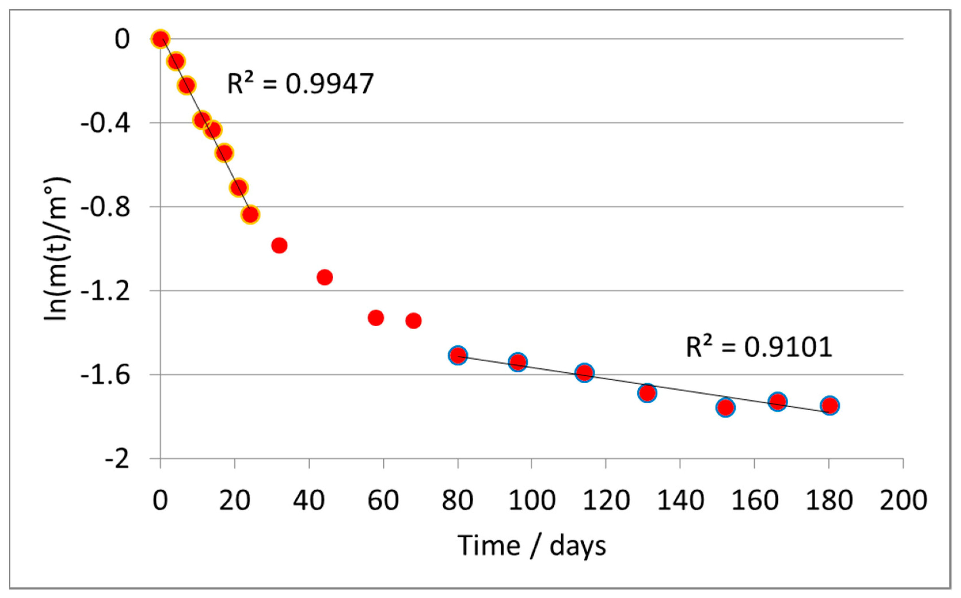
Representing the results according to Equation (4), a substantially linear trend was observed, confirming the validity of the assumption of a first-order kinetics, except for the last points of the test, in which the reaction was substantially complete.
Figure 2 shows the results obtained from the linear regression of the curve according to the first-order model for the A formulate. The last three points, marked in blue, were considered outliers according to a statistical analysis of the deviance of their error (>300% in absolute value), from the mean value of the difference between the value calculated by the regression and the experimental one.
The absolute value of the slope of the line directly provides the value of the kinetic constant k, according to Equation (4). It was calculated as a value of k = 0.0204 ± 0.0010 days−1.
As verification, we calculated the half-life of the polymer, t
1/2. For kinetics of first order, the calculation of the half-life is carried out with the following equation
This result is perfectly in line with the experimental data, thus confirming the correct attribution of the reaction order. Then, the time required to biodegrade the polymer to 90%, 99%, 99.9% is estimated in
Table 1.
The calculated data for the biodegradation of 90% of the material, 116 days, achieved further correspondence with the experimental data. It is noted, as said above, that it is impossible to estimate the time required to reach a 100% conversion for purely mathematic limits with this model, since it would be necessary calculate the ln(0). However, a concentration of residual polymer that is as low as desired can be entered in the formula, as long as it is different from 0.
The marked difference in the time taken for different conversions is due to the non-linear form of the model with respect to the concentration of the substrate. That is, when almost all the reagent is converted, the rate of the reaction slows down considerably, imposing longer times on the biodegradation of the residual material.
A model of enzyme biodegradation based on the Michaelis–Menten equation was also used to reprocess the data, applied in its linearized form according to a Lineweaver-Burk plot, where v is the degradation rate and v
max its maximum value, K
M is the Michaelis constant and [S] is the substrate concentration.
This model led to a non-linear plot for substrate A, denoting that it is unsuitable to correctly fit the data. The elaboration led to a broad estimation of the degradation time with respect to the first-order model. Details are reported in the
ESI, Figure S1, for the interested reader.
3.2. Material B
With an increase in the complexity of the polymer, we expect longer and possibly less complete biodegradation. The curve of biodegradation of formulate B (
Figure 1) indicates an initially faster conversion, which then slows down with respect to sample A.
The same approach was used for data elaboration. In this case, the initial rate of biodegradation was very high, but after approximately 25 days, it underwent an abrupt slowdown, until it became negligible. The application of the same criteria of data-reprocessing throughout the whole experimental field has, however, produced a curve instead of a line, as shown in
Figure 3.
This suggests the inadequacy of the first-order kinetic model in this case. Furthermore, the application of equations of order 0 or 2 did not produce significant improvements (see
Supplementary Information).
Therefore, we adopted a different strategy. We assumed a reaction of order n
and we applied the method of Wilkinson for the determination of kinetic parameters [
22].
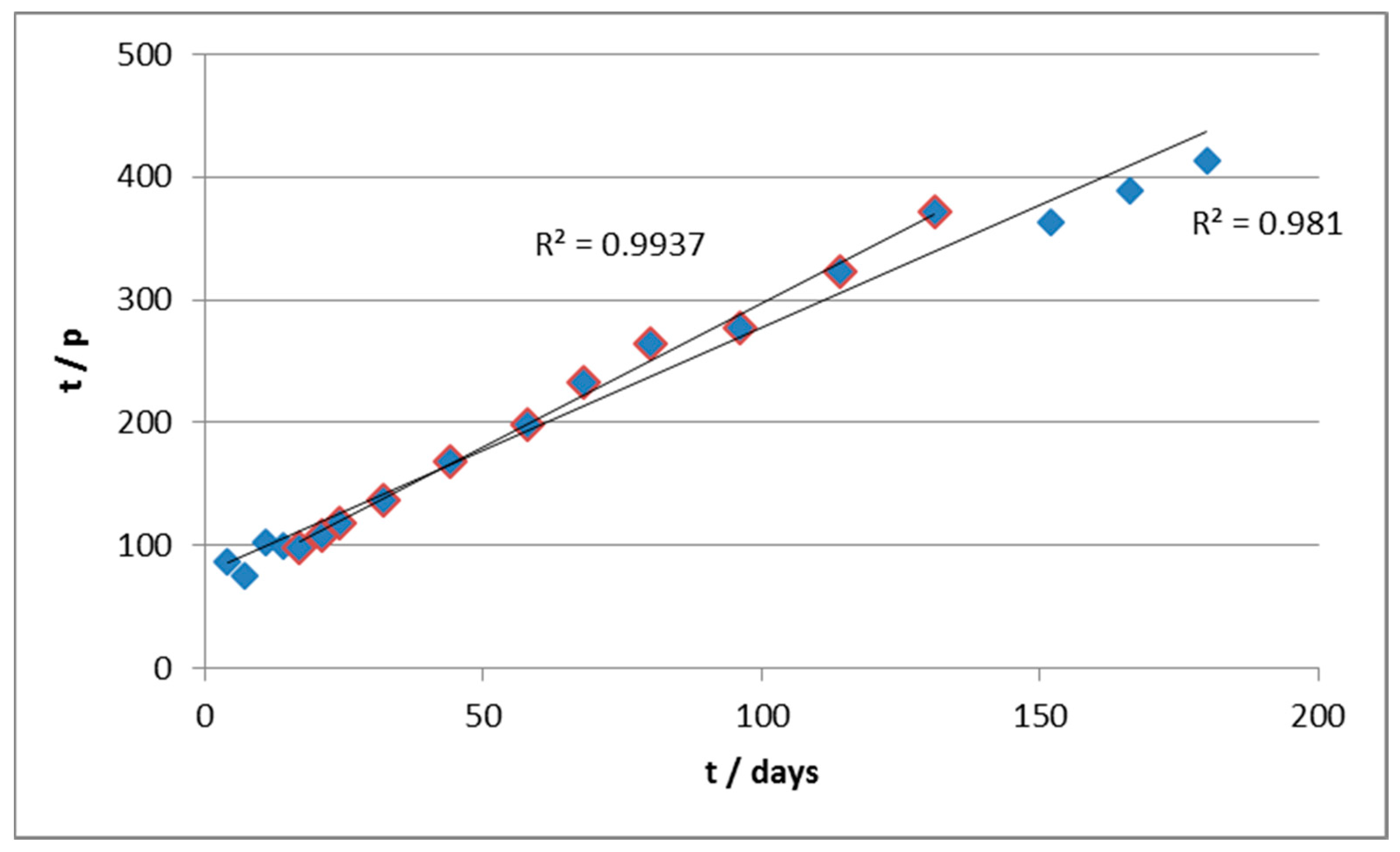
Approximately, it is possible to calculate a parameter p = 1-m/m° and to perform a linear regression of t/p vs. t, as follows
Therefore, the double of the slope of the line provides the estimated reaction order, while it is possible to estimate k from the intercept. According to this approach, we elaborated the kinetics of degradation of material B.
From the values of slope and intercepts, we estimated (
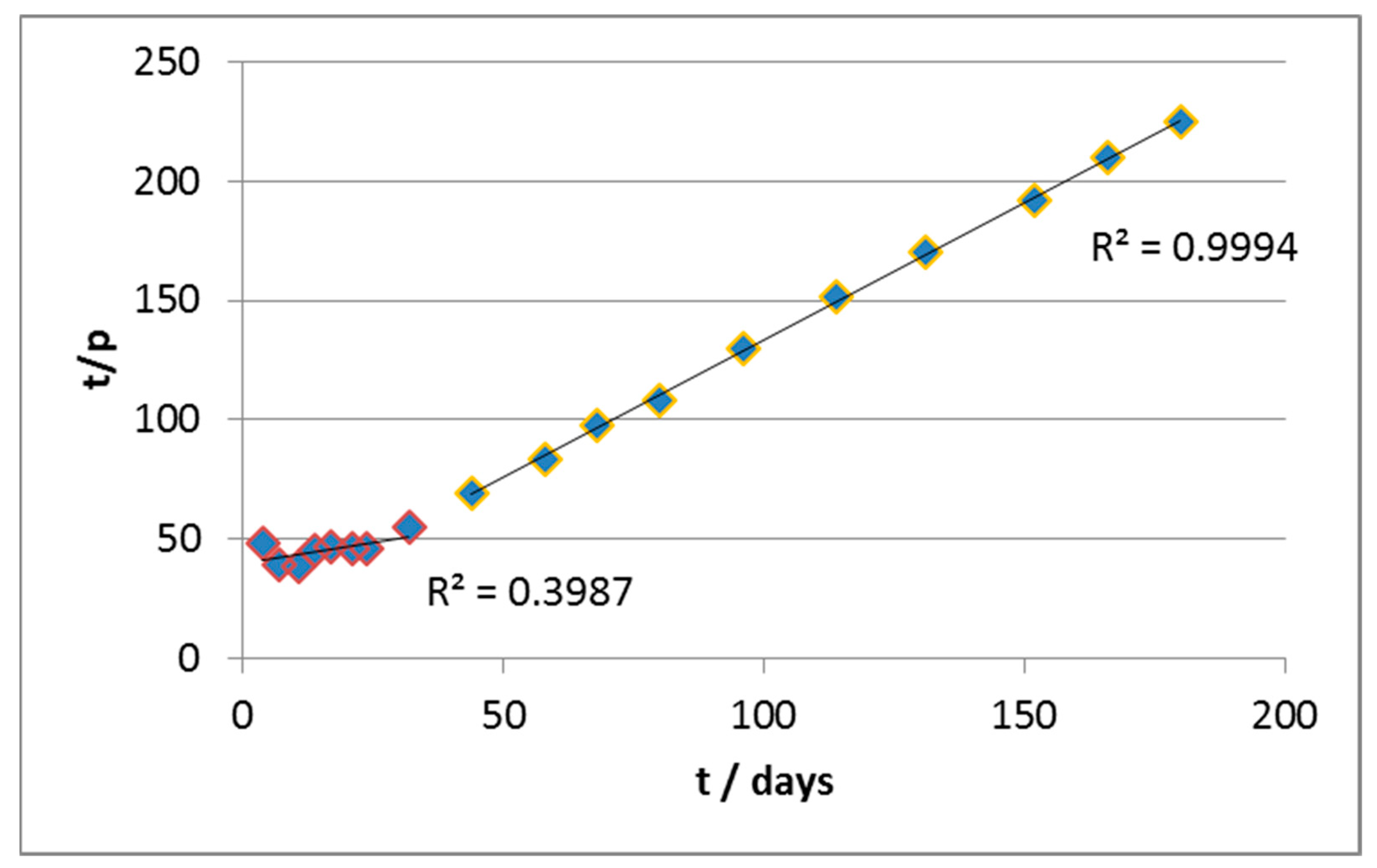
Table 2) the values of n and k in the two curve sections (roughly active before and after 30 days (
Figure 4).
In particular, it can be seen that in the early stages of the biodegradation, the estimated reaction order is <1 (as if there were product inhibition). The kinetics are also quite fast thanks to the relatively high value of k (as compared, for example, to material A) and the abundance of the substrate, which mitigates the slowing effect due to a fractional order of reaction. Notice that, in the first segment, the R2 value of the regression is severely low, partly for the scattered values, but also due to the very small slope of the curve, which is the main reason for the very low value of the correlation coefficient.
In the second section, on the other hand, the apparent order of reaction is higher and this, combined with the progressive consumption of substrate, leads to a significant slowing down of the reaction rate. In parallel, the fact that the curves of biodegradation practically reach a plateau is reflected in a kinetic constant which is orders of magnitude lower with respect to the previous section.
Using these kinetic data, we made two predictions, including the conversion in the experimental field to test the reliability of the model (
Table 3):
From these data, it is evident that the first section (t < 30 days) is effectively described by the model. In the second section, the prevision is reasonable, although underestimated by 8–10%. The kinetic data of the second segment were used to estimate the time of biodegradation to 90%, 99% and 99.9% with the results reported in
Table 1. By contrast, the first-order model underestimates the biodegradation time to achieve 20% conversion and poorly fits the prediction of 70% conversion.
We are interested in the prediction of the ultimate biodegradation, so the most interesting part of the curve is the one at higher times. The first part is also the most dependent on the possible presence of additives and pro-oxidants. The data reported in
Table 3 show that the predicted time for 20% biodegradation is better calculated by the Wilkinson model, even if the almost horizontal fitting curve has a lower correlation coefficient.
Therefore, it is highly recommended to compare the kinetic models, not only for their fitting ability, but for their overall capacity to correctly represent the whole dataset.
Finally, we applied the Michaelis–Menten, zero-order and second-order models also to material B
(see ESI), Figures S4–S6. The reprocessing of the data led to the same problems highlighted for material A.
3.3. Material C
The set of data for the formulate C (
Figure 1) shows only a partial conversion of the polymer at the end of the test and a sharp downturn in reaction rate after the first 20–25 days. There is a rapid digestion of approximately 20% of the initial mass of the polymer and a subsequent slowdown. This could be due to a sequential mechanism of attack, according to which the chain is first broken and is partially eliminated in a more degradable portion, e.g., an aliphatic chain; subsequently, it proceeds with the biodegradation of the less degradable residual, for instance, an aromatic ring, which is considerably more resistant. This may explain the evolution of the curve, which slows down after 30 days, without reaching a net plateau.
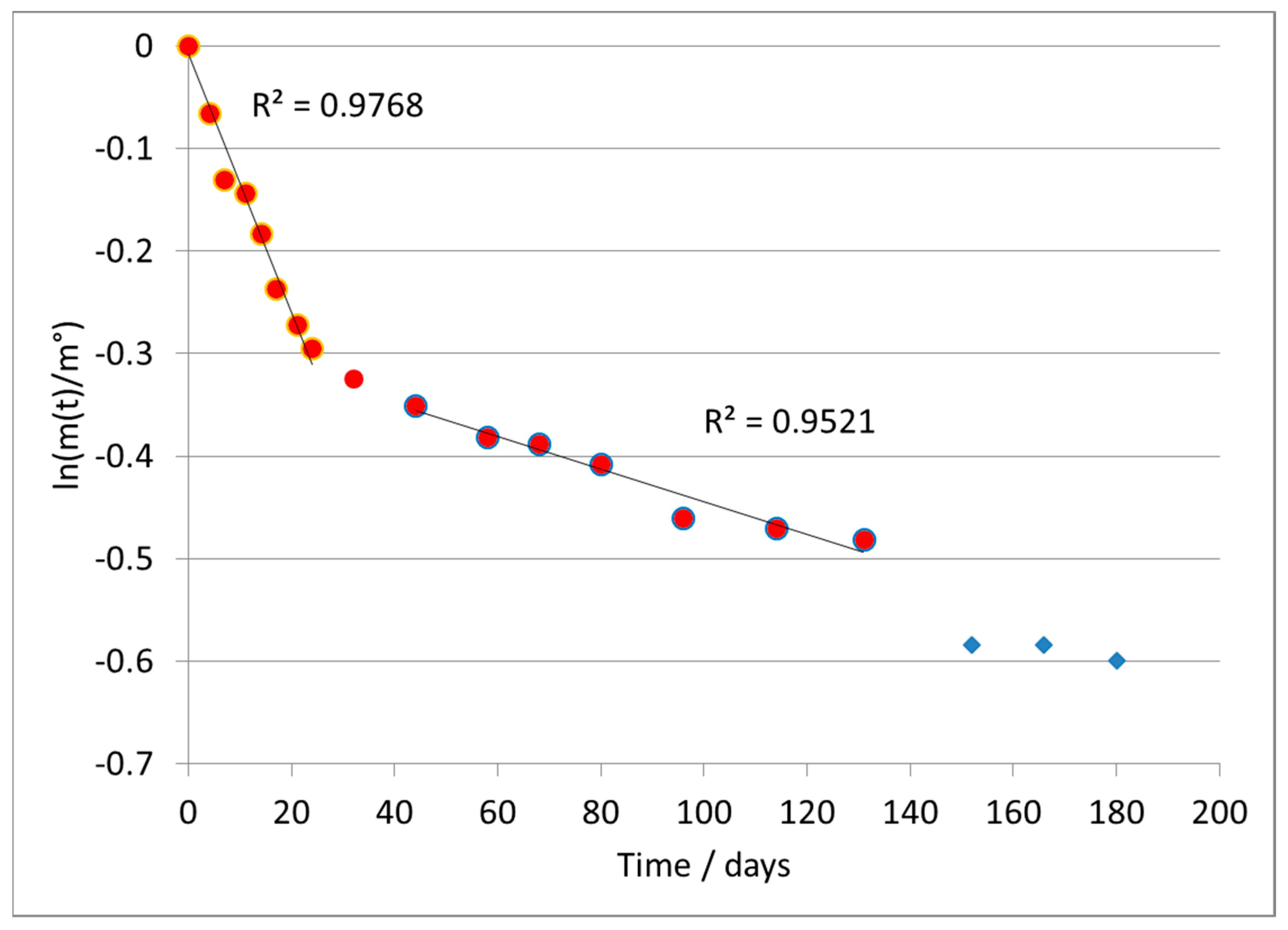
Applying the first-order model (
Figure 5) led again to a broken line, and in this case we separately treated the two branches of the curve.
In particular, we discuss the data of the second branch, since the first section does not clearly represent the rate-determining step of the reaction, as already discussed for previous types of material. The average value of the kinetic constant (second branch) was k = 0.00200 ± 0.00012 days−1.
The calculated halving time using k2 was 345 days, but there are no experimental data to check this value. However, this forecast seems to be reasonable, observing the available experimental data. In fact, the biodegradation of ca. 20–25% of the polymer occurs in ca. 155 days (excluding the first period of 25 days, in which the kinetic was much faster and converted ca. 20% of the substrate). It therefore seems likely that 345 days following the slowest kinetics can lead to 50% conversion.
Accordingly, we estimated the following conversion times for biodegradation of 90%, 99% and 99.9% of the substrate (
Table 1).
We also applied the Wilkinson model to this substrate (
Figure 6). The reprocessing led to an apparent value of reaction order n = 4.2, with values of k in the order of 10
−8 day
−1 mg
−3. Using these data to determine the time taken to reach 20% conversion returns an estimate of 25 days, broadly comparable with the experimental value. However, when one tries to provide the trend in the longer term, the deviations between calculated and experimental data become unacceptable. Even when excluding the last three points, which were again defined as outliers according to statistical analysis of the error distribution, the estimated parameters were n = 5.1 and k in the order of 10
−10 day
−1 mg
−3, leading to overall unreliable predictions. The calculated time for biodegradation of 20% of the substrate was 20.1 days vs. 21 in the experimental, while for 30% biodegradation it was 44.7 days vs. 80 experimental.
This approach was, therefore, abandoned for material C, in spite of the quite good quality of data regression, also testified by the higher R2 value with respect to the first-order model, because it does not allow the weighting of the different branches of the curve, which likely rely on different mechanisms.
The Michaelis–Menten, zero-order and second-order models were also unsatisfactory when applied to this sample
(see ESI), Figures S7–S9.
3.4. General Remarks
This work does not aim to provide evidence for or to discuss the biodegradability behavior of the tested materials, but rather to propose a kinetic approach to the elaboration of the degradability data (collected on whichever material) for a better comparison between different samples and tests.
Polyolefins represent the most widely used polymers, especially in the commercialization of single-use manufacts, such as food and beverage packaging. Pure polyethylene (i.e., not treated or combined with pro-oxidants) is extremely recalcitrant to degradation by abiotic or biotic factors, demonstrating limited mass loss after burial in humid soil for several years. Its resistance is due to concomitant factors. The hydrophobic chain prevents attack and colonization by microbials, which also cannot digest high-molecular-weight entities. Indeed, these molecules cannot enter microbial cells to be digested by intracellular enzymes and they are inaccessible to extracellular enzymes because of their excellent barrier properties. This is even more severe when increasing the crystallinity degree. As an example, UV-irradiation of polyethylene for 16 days before burial in soil produced less than 0.5 wt% carbon after 10 years, while in that without any pretreatment, less than 0.2 wt% CO
2 was observed [
23].
Thus, in order to circumvent this exceptional stability that brings environmental accumulation, different strategies have been formulated to improve the biodegradability of plastic-based objects prepared from conventional polymers, hence maintaining their functionality and processing advantages.
Possible pretreatments and the use of additives deeply modify the biodegradation of the material, in order to improve the abiotic steps of oxidation and to favour subsequent biotic action. For instance, a high-density PE film was chemically treated by immersion into KMnO
4/HCl at for 8 h and 10% citric acid for 8 h at 45 °C. The HDPE degradation gradually increased from 9.4 to 20.8%, indicating synergism between biotic and abiotic factors [
5]. Various transition-metal-based additives (traces of Mn, Fe, Co, Ti, e.g., as stearate or oleate) are also well known to improve the biodegradability thanks to an increase in the hydrofilicity and preliminary oxidation of the chain. A total of 70% degradation of a pre-oxidized high-molecular-weight polyethylene sample has been reported after 15 days of treatment with P. chrysosporium strain MTCC-787 [
24]. Furthermore, the TDPA technology combines a transition metal carboxylate and an aliphatic poly (hydroxyl–carboxyl acid) [
25]: samples of low-density PE films were tested with ca. 50–60% degradation after 18 months in soil. After 70 weeks, no fragments were collected from the soil [
26]. Moreover, oxygenated compost columns at 50 °C to degrade PE films after fragmentation returned 60% mineralization after 400 days, whereas thermoformed PP films at 60 °C mineralized up to 60% in 700 days. The difference in degradation times was attributed to the different film thicknesses, since another important parameter is size [
27].
It is clear that the search for a solution to the contingent issue of the scarce or nil biodegradability of packaging polymers has led to important results, but a plethora of pro-degradants are commercially available, as recently listed [
14], and may be found in commercial formulates [
5,
28], often without clear indication: this further jeopardises the possibility of predicting the ultimate biodegradation time of such formulates.
In addition, the interest in the development of biodegradable plastics is rapidly raising, with a lot of composite materials that increase the degradability of the manufacts relying on more intrinsically degradable polymers where feasible (e.g., PLA), or on blending classic polyolefins with a biodegradable material (e.g., starch), often in concomitance with pro-oxidants. This wide variability of formulations is often unrecognizable in the disposed manufact, which reports only general indications on the base material (polyethylene, polypropylene, polystyrene, etc.) and on disposal prescriptions. Therefore, a more systematic approach towards degradation testing may help in comparing different formulations. We here propose a simplified kinetic modelling that may be useful to estimate the ultimate degradation time through modelling the aerobic biodegradation tests collected through a standardized method, whatever the tested material. This approach can be used to evaluate every batch of data of CO2 evolution vs. time.
Very wide formulations are currently commercialised. The presence of degradation enhancers may be one of the possible causes of the different degradation rates in the obtained curves. However, this does not affect the modelling methods, since promoters can have different effects. They can facilitate colonisation and attack by microorganisms or render the surface more prone to degradation (e.g., increasing hydrophilicity). In this case, one should see an overall increase in rate, but the mechanism remains practically the same and a pattern similar to material A is expected. In case the promoter instead implies limited durability (e.g., it degrades itself or gets lost in time, e.g., by leaching), one can expect an enhanced rate at the beginning of testing for the whole life of the material, so the overall curve manifests different slopes in time (as for materials B and C); in such a case, the expected ultimate degradation time should be considered from the slowest portion of the curve. The same variation in the curve is expected when the material is constituted of portions of the chain that can be more promptly attacked and portions that are harsher to degrade.
The particle size also deeply affects the degradation rate; examples of the testing of materials with different grain sizes can be found in the literature [
11,
13]. Fine comminution exposes more surface area and leads to easier formation of the biofilm, which is ultimately responsible for the biodegradation. Thus, the very small particles used in the present experiments cannot be compared with the rates observed for films, layers, etc. The wide variability of conditions and formulations contributes to the miscellaneous results landscape, making it really difficult to draw a general conclusion on the biodegradability of a material. Therefore, besides using standardized testing protocols, the use of well-defined data elaboration models would help obtain more uniform and comparable results.
The present data were elaborated using various kinetic models, highlighting their strengths and limitations. In every case, the elaboration was based on the best available kinetic models in the state of the art. The choice of the most appropriate kinetic models was made not only on the basis of the examination of the results, but also in light of some indications found in the literature. Specifically, A. Models et al. [
29] underline that the biodegradation of polymeric materials in a homogeneous phase is properly describable by means of a Michaelis–Menten type kinetic model (enzyme kinetics), which is not entirely appropriate or properly extendable to the case of the aerobic final biodegradation of plastic materials under controlled composting conditions (see
ESI). The application of a kinetic model of the first order represented a better representation of the results.
In support of this, another investigation [
30] adopted a first-order kinetics approach. The authors also consider biodegradation that is possible via reactions in series, always of first order, when a period of initial induction is present in the formation of CO
2. In other studies, a purely empirical strategy was adopted, by interpolating the data of CO
2 formation as a function of time with mathematical models (not mechanistic) [
31]. In such a case, it would be possible to calculate the time required for the formation of the theoretical amount of CO
2 corresponding to complete biodegradation of the polymer. It should be recalled, however, that the models obtained by pure fitting of experimental data, not based on a verified mechanism of reaction, are usable for the forecasts within the adopted experimental field and not for extrapolation to a final degradation time longer than the experiment. Therefore, they are not the best option for long-term forecasting.
