From Physical to Virtual Sensors: VSG-SGL for Reliable and Cost-Efficient Environmental Monitoring

Abstract

Reliable environmental monitoring in remote or sparsely instrumented regions is hindered by the cost, maintenance demands, and inaccessibility of dense physical sensor deployments. To address these challenges, this study introduces VSG-SGL, a unified virtual sensor generation framework that integrates Sparse Gaussian Process Regression (SGPR) and Bayesian Ridge Regression (BRR) with deep generative learning via Variational Autoencoders (VAE) and Conditional Tabular GANs (CTGAN). Real meteorological datasets from multiple South Korean cities were preprocessed using thresholding and Isolation Forest anomaly detection and evaluated using distributional alignment (KDE) and sequence-learning validation with BiLSTM and BiGRU models. Experimental findings demonstrate that VAE-augmented virtual sensors provide the most stable and reliable performance. For temperature, VAE maintains predictive errors close to those of BRR and SGPR, reflecting the already well-modeled dynamics of this variable. In contrast, humidity and wind-related variables exhibit measurable gains with VAE; for example, SGPR-based wind speed MAE improves from 0.1848 to 0.1604, while BRR-based wind direction RMSE decreases from 0.1842 to 0.1726. CTGAN augmentation, however, frequently increases error, particularly for humidity and wind speed. Overall, the results establish VAE-enhanced VSG-SGL virtual sensors as a cost-effective and accurate alternative in scenarios where physical sensing is limited or impractical.

1. Introduction

Environmental monitoring in remote or constrained regions, such as mountainous terrains, offshore platforms, and sparsely populated areas, faces persistent challenges due to the high cost, limited accessibility, and complex maintenance demands of deploying dense physical sensor networks. In such contexts, virtual sensors, also referred to as soft or computational sensors, provide a promising alternative by estimating environmental variables through data-driven models rather than direct physical measurement. These virtual sensors leverage existing sensor observations, contextual information, and statistical or generative learning frameworks to infer measurements at locations where physical deployment is either impractical or prohibitively expensive.

Conventional environmental monitoring systems primarily rely on large-scale sensor deployments, yet their scalability is restricted by financial and logistical constraints [1]. Physics-based simulations and traditional supervised learning approaches have been adopted to compensate for sparse data availability, but their performance often degrades in highly dynamic or heterogeneous environments [2]. In particular, incomplete datasets or sensor outages significantly reduce prediction accuracy and reliability. To overcome these issues, virtual sensing has emerged as a cost-effective and scalable strategy for extending monitoring coverage, mitigating missing data, and enhancing the resilience of environmental observation systems.

The main advantages of virtual sensors over conventional methods can be summarized as follows:

• Cost Efficiency: reduction in expenses associated with hardware procurement, calibration, and long-term maintenance.
• Extended Coverage: reliable estimation of variables in hazardous, inaccessible, or sparsely instrumented regions.
• Real-Time Inference: continuous predictions that support timely monitoring and adaptive decision-making.
• Fault Tolerance: ability to fill missing data gaps and provide redundancy when physical sensors fail.

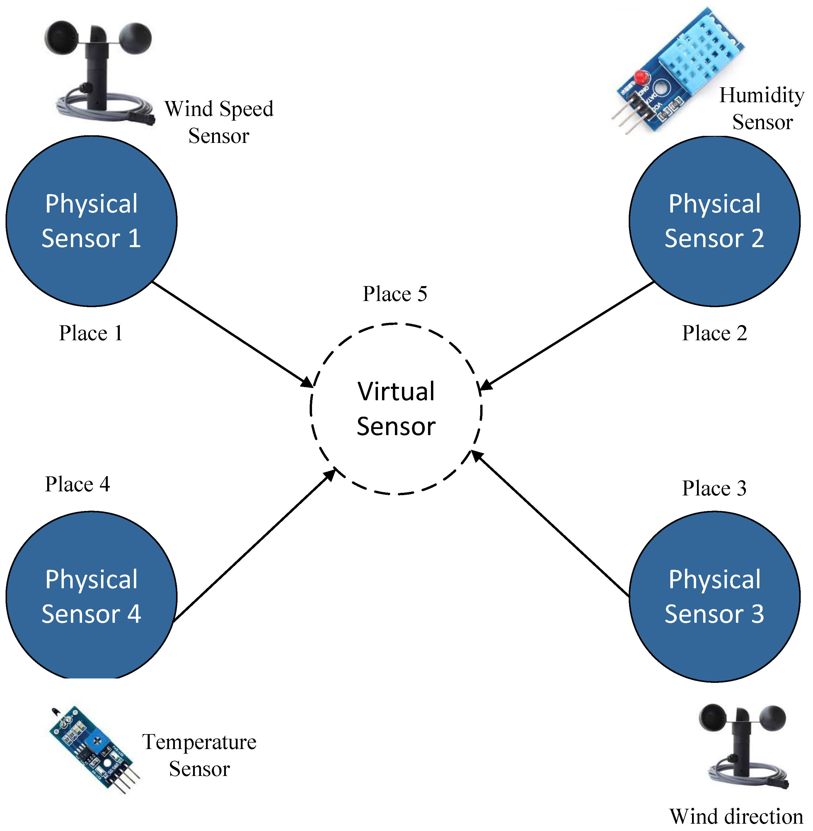
Figure 1 illustrates a representative case where a virtual sensor (Place 5) is inferred using nearby physical sensors measuring wind speed, humidity, temperature, and solar radiation. This example highlights how distributed observations can be combined to enhance environmental monitoring.

Recent advances in data-driven modeling, particularly deep generative frameworks such as VAEs [3] and CTGANs [4], have demonstrated strong potential for producing high-fidelity synthetic data that complements sparse or noisy sensor observations. These models are especially valuable when regression-based approaches struggle under limited data conditions. However, most existing virtual sensor frameworks remain fragmented: statistical regression, generative modeling, and validation are seldom unified within a single end-to-end pipeline.

To address this gap, we propose a novel framework, termed VSG-SGL (Virtual Sensor Generation via Statistical and Generative Learning). The framework integrates SGPR [5] and BRR [6] for statistical estimation with VAE- and CTGAN-based augmentation, yielding a multi-stage architecture capable of producing reliable and diverse virtual sensor data. Real-world environmental datasets from multiple South Korean cities are employed to evaluate the framework. Data preprocessing involves thresholding and Isolation Forest-based outlier detection, followed by generative augmentation to enhance dataset completeness and variability.

The generated virtual sensor data is validated through both the temporal correlation analysis and the predictive assessments using sequential models (BiLSTM and BiGRU). Results indicate that, in many cases, virtual sensors enhanced with generative learning can achieve predictive accuracy comparable to, or surpassing, physical sensors.

The novelty of the proposed VSG-SGL framework lies in its unified design that integrates statistical regression models (SGPR/BRR), deep generative models (VAE, CTGAN), and sequence-learning-based validation using BiLSTM/BiGRU into a cohesive pipeline for virtual sensor generation. Unlike prior virtual sensing approaches that rely on a single class of models, VSG-SGL establishes a multi-stage synergy: regression models provide physically grounded baseline estimates, generative models enrich them by capturing nonlinear and distributional variations, and sequence-learning models validate temporal consistency and predictive reliability. This layered workflow systematically corrects model bias, enhances data realism, and ensures that the final virtual sensors exhibit both statistical fidelity and functional coherence. Such an integrated and reproducible architecture has not been previously explored in the virtual environmental sensing literature.

The key contributions of this study are summarized as follows:

• Development of the VSG-SGL Framework: Introduction of a unified and synergistic virtual sensor generation pipeline that seamlessly combines statistical regression (SGPR, BRR) with deep generative learning (VAE, CTGAN), enabling improved modeling of nonlinear and sparse environmental variables.
• Structured and Multi-Stage Data Augmentation Pipeline: Design of a two-tier augmentation strategy: VAE and CTGAN to strengthen sensor datasets and compensate for missing or inconsistent physical measurements.
• Comprehensive and Measurable Validation Protocol: Establishment of a dual-validation process that evaluates (i) distributional alignment through KDE, KS-statistics, and correlation analysis and (ii) temporal predictive performance through BiLSTM and BiGRU models to ensure functional realism of the generated virtual sensors.
• Extensive Real-World Evaluation: Demonstration of the effectiveness, stability, and scalability of the VSG-SGL framework using real environmental datasets from multiple South Korean cities, highlighting its potential as a reliable and cost-efficient alternative to dense physical sensor deployments.

Table 1. Techniques for generating virtual sensor data under limited or no physical data scenarios.

Scenario	Category	Method	Description	Tools
Limited Sensor Data	Supervised Learning	Regression [7]	Learns relationships from existing observations to predict missing values.	Linear/Polynomial Regression, Scikit-learn
		Bagging [8]	Improves accuracy by aggregating predictions from multiple learners.	Decision Trees, Random Forests
	Data Augmentation	GANs [9]	Learns data distribution to synthesize additional samples.	TensorFlow, PyTorch
		VAEs [10]	Generates samples from latent representations of the dataset.	TensorFlow, PyTorch
No Sensor Data Available	Simulation-Based	Physics-Based [11]	Employs governing equations to simulate sensor behavior.	MATLAB, COMSOL Multiphysics
		Bayesian Modeling [12]	Infers distributions using priors and expert-driven knowledge.	PyMC, Stan
	Hybrid Modeling	AI-Enhanced Physical Models [13]	Integrates physical models with AI for robust estimation.	AI Frameworks + Simulation Tools

provides an overview of representative methods for virtual sensor generation under scenarios with limited or no physical data availability.

2. Literature Review

Virtual sensors have gained significant attention across multiple domains due to their ability to replicate physical sensor functionality using computational techniques. They are particularly useful when deploying physical sensors is infeasible, costly, or constrained by terrain and infrastructure limitations [14,15,16]. The literature on virtual sensing highlights several complementary approaches that have been developed to overcome sparse data availability and sensor inaccessibility. These can broadly be grouped into supervised learning, generative augmentation, physics-informed modeling, deep neural and transformer-based architectures, anomaly detection methods, and hybrid frameworks.

Early studies employed supervised learning techniques, where regression-based models such as BRR and SGPR were used to capture functional relationships between correlated sensor variables. Ensemble-based methods, including Random Forests and Gradient Boosting, further improved robustness by aggregating multiple weak learners [17]. Support Vector Machines (SVMs) showed strong generalization in low-data regimes [18], while Gaussian Processes allowed uncertainty-aware predictions in sparse and noisy environments [19]. These techniques have been successfully deployed in industrial automation, HVAC systems, and meteorological monitoring.

As data scarcity persisted, generative augmentation became increasingly important. VAEs and CTGANs were used to learn complex, nonlinear distributions in environmental and industrial data. CTGANs, designed for tabular modalities [20], demonstrated strong performance in preserving marginal and joint distributions, making them suitable for virtual sensing and missing-sensor recovery tasks. GAN-based methods further showed effectiveness in IoT data imputation and environmental signal reconstruction [21], while VAE-based frameworks improved reliability forecasting and water-quality monitoring [10,22]. These approaches addressed overfitting risks under limited or imbalanced datasets.

Physics-driven models provided an alternative when ground-truth measurements were unavailable. Simulations such as Computational Fluid Dynamics (CFD), Finite Element Analysis (FEA), and system dynamics models offered physically consistent sensor approximations in agriculture, environmental systems, and renewable energy forecasting [23,24,25]. Hybrid physics, ML virtual sensors, such as physics-informed neural networks (PINNs) and Kalman filter–assisted learning, have recently emerged to combine interpretability with data-driven adaptability [2,26]. These methods represent cutting-edge developments in virtual sensing and provide a balanced alternative between full-simulation and purely data-driven approaches.

The development of advanced sequence models further expanded the capabilities of virtual sensors. Recurrent neural networks (LSTM, GRU) were used to model temporal dependencies in environmental and industrial processes [27,28]. More recently, transformer-based architectures, including dual-attention RNNs and dual-scale transformers, have demonstrated superior accuracy in long-range time-series modeling [29,30]. These methods have been used in air-quality prediction, energy forecasting, and weather sensor reconstruction. Additionally, several benchmark datasets, such as the UCI Air Quality Dataset [31], the Beijing PM2.5 dataset [32], and NOAA Integrated Surface Dataset (ISD) [33], serve as commonly used baselines in environmental virtual sensing research, though many works rely on domain-specific private datasets.

Anomaly detection is another essential component of virtual sensing. Isolation Forest, One-Class SVM, and Local Outlier Factor (LOF) are widely used for filtering corrupted sensor readings [34,35,36]. Recent studies also explore deep anomaly detection through autoencoders and reconstruction-based neural methods for environmental signals [37]. These tools ensure that noisy or malfunctioning sensor data does not propagate through the virtual sensor pipeline.

Overall, prior research demonstrates significant progress in virtual sensing across methodological categories. However, existing frameworks typically focus on isolated components, statistical estimation, generative augmentation, or sequence modeling without offering a unified and reproducible workflow. Moreover, the influence of generative augmentation on downstream predictive models is rarely examined in a measurable manner. Addressing these gaps, our proposed VSG-SGL framework integrates SGPR, BRR, VAE, and CTGAN in a multi-stage architecture validated using KS-statistics, correlation analysis, and BiLSTM/BiGRU consistency evaluation. A consolidated overview of representative virtual sensor approaches across these categories is provided in

Table 2. Summary of representative approaches in virtual sensor development.

Category	Study/Model	Description	Domain
Supervised Learning	Regression, Bagging, SVM, GPs [7,17,18,19,38,39,40]	Estimate sensor outputs from available data; ensemble methods improve robustness; GPs provide uncertainty quantification.	Industrial automation, smart buildings, environmental monitoring
Generative Augmentation	GANs, CTGANs, VAEs [10,21,22,41]	Learn data distributions to create synthetic samples; enhance diversity and robustness under limited or imbalanced datasets.	IoT reliability, chemical process monitoring, water quality, industrial monitoring
Simulation-Based Models	CFD, FEA, System Dynamics [23,24,25]	Physics-driven models simulate sensor behavior in the absence of data, ensuring physical consistency but with scalability challenges.	Agriculture, energy systems, climate modeling
Deep Learning and Transformers	DNN, LSTM, GRU, DA-RNN, Transformers [27,28,29,30]	Capture nonlinearities and long-range dependencies in time-series data for real-time virtual sensing.	Automotive emissions, industrial process control
Hybrid and Ensemble Models	Random Forest, PCA+RNN, EMD+SVM, Kalman Filtering [2,26,42,43,44,45,46]	Integrate physics-based and AI-driven models to enhance interpretability and robustness in sparse-data environments.	Automotive monitoring, robotics, water quality, industrial monitoring

, highlighting the evolution of methods and their application domains.

3. Proposed VSG-SGL Methodology

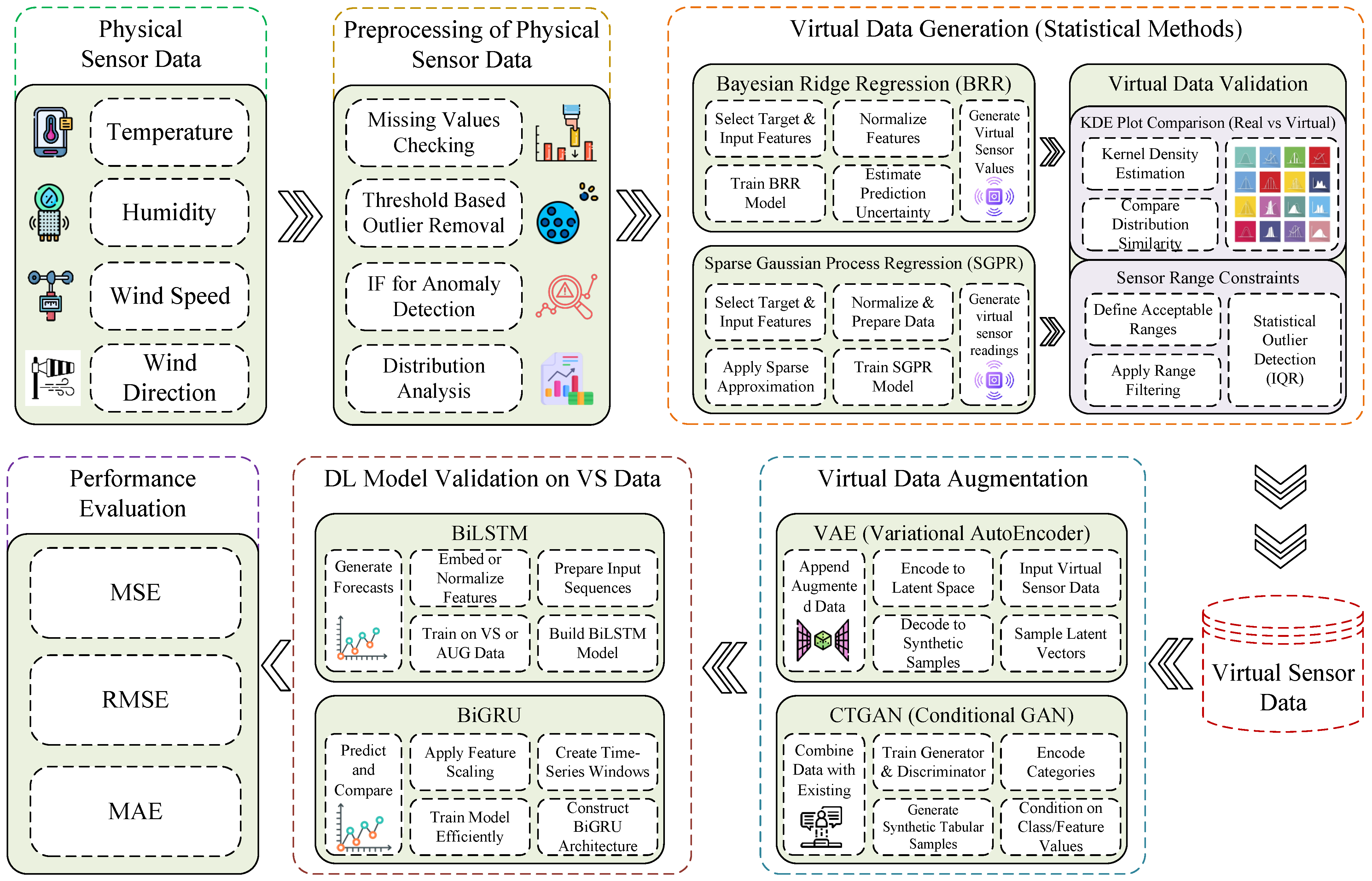
The proposed VSG-SGL framework establishes a complete pipeline for developing reliable virtual sensors using hybrid statistical, generative, and deep learning approaches. The process begins with physical sensor data, including temperature, humidity, wind speed, and wind direction, which undergoes rigorous preprocessing. Missing values are imputed, and noisy or abnormal observations are removed through threshold-based filtering and the Isolation Forest algorithm. Next, statistical learning methods, namely BRR and SGPR, are employed to generate baseline synthetic sensor values in situations where real measurements are sparse or unavailable. To ensure that the generated values remain physically meaningful, distributional validation is performed using sensor-specific value-range constraints.

To further enrich the dataset and improve downstream learning robustness, advanced data augmentation modules, VAE and CTGAN, are applied. These models add variability while preserving the core statistical properties of the original data. All generated and augmented datasets are subsequently used to train deep learning-based virtual sensors, specifically BiLSTM and BiGRU architectures. To ensure the stability and generalizability of the reported performance, a K-Fold cross-validation strategy is integrated into the evaluation pipeline. For each sensor variable and each model variant, the dataset is partitioned into k = 5 folds. This prevents overfitting to a single split and provides a statistically reliable estimate of the virtual sensors’ performance.

Finally, the predictive results from all configurations, including baseline statistical models, augmented models, and deep learning models, are evaluated using Mean Absolute Error (MAE), Mean Squared Error (MSE), and Root Mean Squared Error (RMSE) to quantify prediction accuracy and error propagation across different virtual sensor setups. Figure 2 illustrates the overall VSG-SGL architecture.

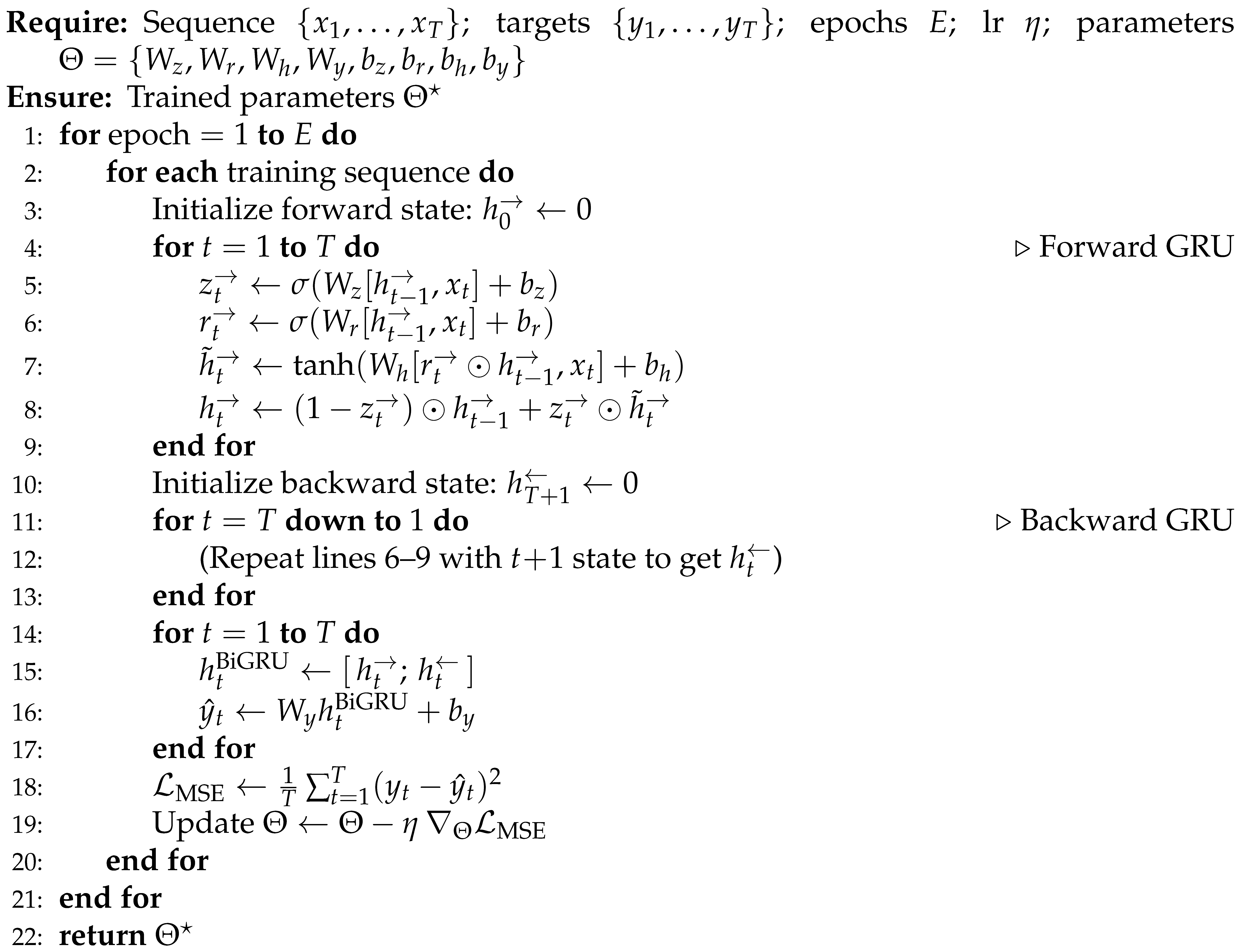
Moreover, Algorithm 1 initiates by generating virtual sensor data using BRR and SGPR, trained on physical measurements. This virtual data is then validated within the defined sensor ranges. Subsequently, VAE and CTGAN models are used to augment the virtual dataset further. The resulting dataset, comprising physical, virtual, and augmented data, is used to train BiLSTM and BiGRU models for univariate prediction. Finally, the trained models are evaluated using standard performance metrics, including MSE, RMSE, and MAE.

Algorithm 1 VSG-SGL: Virtual Sensor Generation and Smart Generalization Framework

3.1. Physical Sensor Dataset

The dataset employed in this study comprises high-resolution meteorological measurements captured from nine physical sensor nodes deployed across diverse microclimatic zones within Gwacheon City, South Korea. Each node records temperature, humidity, wind direction angle, and wind speed every 10 min, generating approximately 4000–4300 samples per station per month, with precise timestamps (modifie_at) and spatial coordinates encoded in WGS-84 (location_4326). Since the sensors were installed, calibrated, and maintained directly, the whole spatial–temporal structure of the data can be reproduced without relying on an external agency. However, for comparison and validation, regional weather information was also referenced from the Korea Meteorological Administration (KMA) public portal (access on 10 March 2025). (https://data.kma.go.kr). The nine stations are spaced approximately 0.5–2 km apart across roadside, residential, open-space, and slightly elevated environments, enabling natural variation in shading, terrain influence, wind channeling, humidity pockets, and urban heat island effects to be reflected in the dataset. This rich spatiotemporal configuration enables the proposed VSG-SGL framework to capture localized atmospheric dynamics critical for environmental forecasting and disaster management modeling. A detailed description of all variables and sensor parameters is provided in

Table 3. Description of physical sensor data attributes.

#	Sensor Field	Data Type	Description
1	Timestamp	Temporal (datetime)	Records the date and time at which the sensor measurement was taken.
2	Temperature	Continuous (float)	Air temperature measured in degrees Celsius (°C).
3	Humidity	Continuous (float)	Relative humidity represented as a percentage (%).
4	Wind Direction	Continuous (float)	Average wind direction in degrees (0–360°).
5	Longitude	Continuous (float)	Sensor’s geographic longitude coordinate.
6	Latitude	Continuous (float)	Sensor’s geographic latitude coordinate.

.

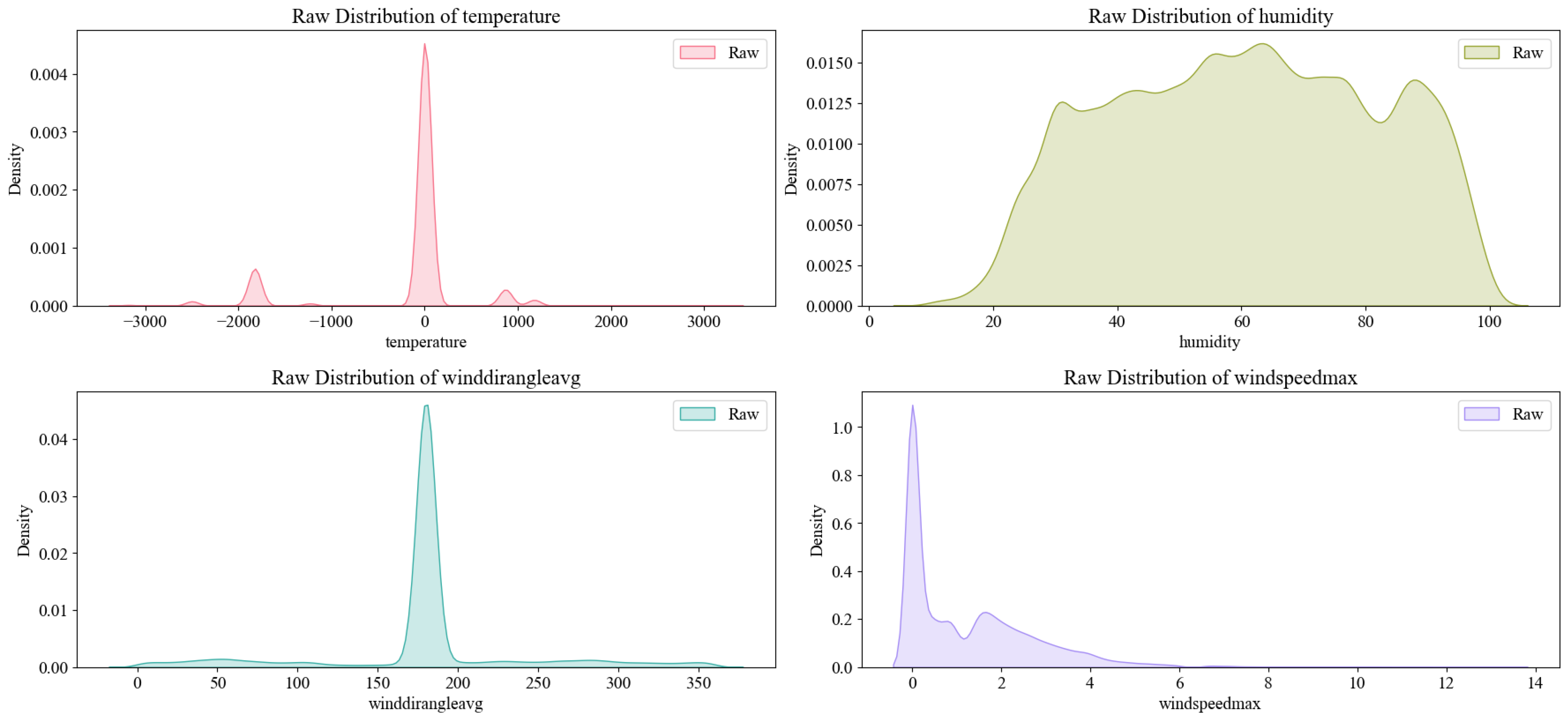
The raw data distributions in Figure 3 reveal substantial anomalies and extreme outliers in temperature, wind direction, and wind speed, justifying the need for systematic preprocessing. These irregularities distort statistical properties such as mean, variance, and modality, which would negatively impact downstream learning. Presenting these distributions clarifies the extent of noise in the original measurements and establishes a quantitative baseline before applying thresholding and Isolation Forest–based outlier removal.

3.2. Data Preprocessing

Real-world sensor data often contains anomalies such as missing values, physically impossible readings, or spurious noise caused by hardware malfunctions, environmental interference, or transmission errors. To ensure the reliability of downstream modeling, we adopt a structured preprocessing pipeline consisting of four main steps: missing value detection, threshold-based outlier removal, Isolation Forest anomaly detection, and distributional analysis.

3.2.1. Missing Value Detection

Let the raw dataset be represented as

$$D=\{x_{i,j}\mid i=1,2,\dots ,N;j=1,2,\dots ,M\},$$

(1)

where $x_{i,j}$ denotes the value of the j-th feature for the i-th observation, N is the number of samples, and M is the number of features (temperature, humidity, wind direction, and wind speed).

The missing values are identified using an indicator function:

$$\delta \left(x_{i,j}\right)=\left\{\begin{array}{cc}1,\hfill & \mathrm{if}{x}_{i,j}\mathrm{is}\mathrm{missing},\hfill \\ 0,\hfill & \mathrm{otherwise}.\hfill \end{array}\right.$$

(2)

The overall missing value ratio for feature j is defined as:

$${\mu }_j={\displaystyle \frac{{\sum }_{i=1}^N\delta \left(x_{i,j}\right)}{N}}.$$

(3)

Features or samples exceeding a pre-defined threshold ${\tau }_{\mathrm{miss}}$ (e.g., 10%) are flagged for imputation.

Once missing values are detected, we apply k-Nearest Neighbors (KNNs) imputation to estimate them based on the similarity between samples. The principle is that observations with similar feature values are likely to have similar missing values.

For a given missing entry $x_{i,j}$, we first compute the distance between the i-th sample (with the missing value excluded) and every other complete sample r:

$$d(i,r)=\sqrt{{\displaystyle \sum _{\begin{array}{c}m=1\\ m\ne j\end{array}}^M}{\left(x_{i,m}-x_{r,m}\right)}^2},$$

(4)

where $d(i,r)$ is the Euclidean distance between sample i and sample r based on all available features except the missing one.

The $kNN$s of sample i with respect to feature j are then selected:

$${\mathcal{N}}_k(i,j)={\mathrm{argmin}}_{r\in \{1,\dots ,N\},r\ne i}^{k}d(i,r).$$

(5)

The imputed value ${\widehat{x}}_{i,j}$ is computed as the weighted average of the neighbors’ values:

$${\widehat{x}}_{i,j}={\displaystyle \frac{{\sum }_{r\in {\mathcal{N}}_k(i,j)}{w}_{i,r}·x_{r,j}}{{\sum }_{r\in {\mathcal{N}}_k(i,j)}{w}_{i,r}}},$$

(6)

where the weights are defined as the inverse distance:

$$w_{i,r}={\displaystyle \frac{1}{d(i,r)+ϵ}},$$

(7)

with $ϵ$ being a small constant to prevent division by zero.

Thus, missing values are imputed by leveraging information from the k most similar observations, ensuring that the reconstructed dataset maintains coherence with the underlying data distribution.

3.2.2. Threshold-Based Outlier Removal

Threshold-based filtering eliminates values outside the physically valid range of each sensor. For feature j, with acceptable lower and upper bounds $[L_j,U_j]$, each observation must satisfy:

$$x_{i,j}\in [L_j,U_j].$$

(8)

The filtered dataset $D^{\prime }$ is expressed as:

$$D^{\prime }=\{x_{i,j}\in D\mid L_j\le x_{i,j}\le U_j\}.$$

(9)

For example, the valid range for temperature was set to −10 °C ≤ T ≤ 22 °C, and for humidity $20\%\le H\le 100\%$. Observations outside these ranges were discarded.

3.2.3. Isolation Forest-Based Anomaly Detection

To refine the dataset further, we employ the Isolation Forest algorithm, which isolates anomalies by constructing random binary trees. Given a sample x, the anomaly score $s(x,n)$ is defined as:

$$s(x,n)=2^{-{\displaystyle \frac{E\left(h\right(x\left)\right)}{c\left(n\right)}}},$$

(10)

where:

• $h\left(x\right)$ is the path length of sample x in the isolation tree,
• $E\left(h\right(x\left)\right)$ is the expected path length averaged over all trees,
• $c\left(n\right)=2H(n-1)-\frac{2(n-1)}{n}$ is the average path length of unsuccessful searches in Binary Search Trees, with $H(·)$ being the harmonic number and n the subsample size.

A data point is classified as an anomaly if:

$$s(x,n)\ge {\tau }_{\mathrm{IF}},$$

(11)

where ${\tau }_{\mathrm{IF}}$ is an anomaly threshold (commonly ${\tau }_{\mathrm{IF}}=0.5$).

3.2.4. Distributional Analysis

After anomaly removal, the distributional characteristics of each feature are assessed. The empirical probability density function (PDF) of feature j is estimated using KDE:

$${\widehat{f}}_j\left(x\right)={\displaystyle \frac{1}{Nh}}\sum _{i=1}^{N}K\left({\displaystyle \frac{x-x_{i,j}}{h}}\right),$$

(12)

where $K(·)$ is the kernel function (Gaussian in this study) and h is the bandwidth parameter. This ensures that the refined data preserves realistic statistical properties and aligns with expected sensor behavior.

The above multi-step pipeline, comprising missing value detection, threshold-based filtering, Isolation Forest refinement, and KDE-based distribution analysis, ensures that the cleaned dataset is both statistically reliable and physically valid, forming a robust foundation for virtual sensor generation.

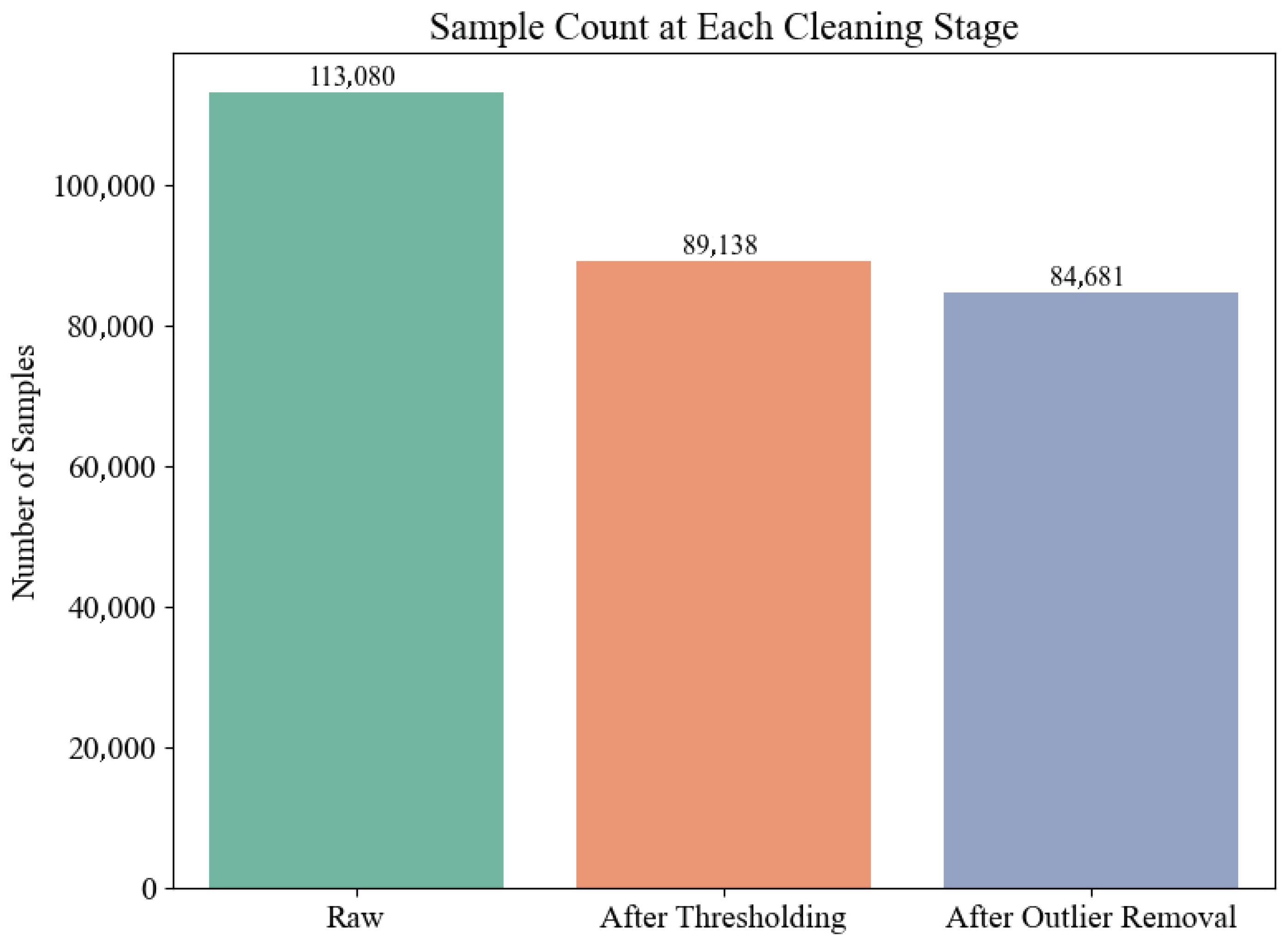
The impact of each cleaning step is summarized in Figure 4, which shows that the dataset was reduced from 113,080 raw samples to 89,138 samples after threshold-based filtering, and finally to 84,681 samples following Isolation Forest refinement. This corresponds to the removal of physically impossible readings, followed by approximately 4.5% anomaly suppression across all sensors. Temperature and wind speed exhibited the highest anomaly rates, while humidity and wind direction remained comparatively stable. These measurable reductions confirm that the preprocessing pipeline systematically eliminates corrupted observations while preserving the statistical integrity of genuine sensor behavior.

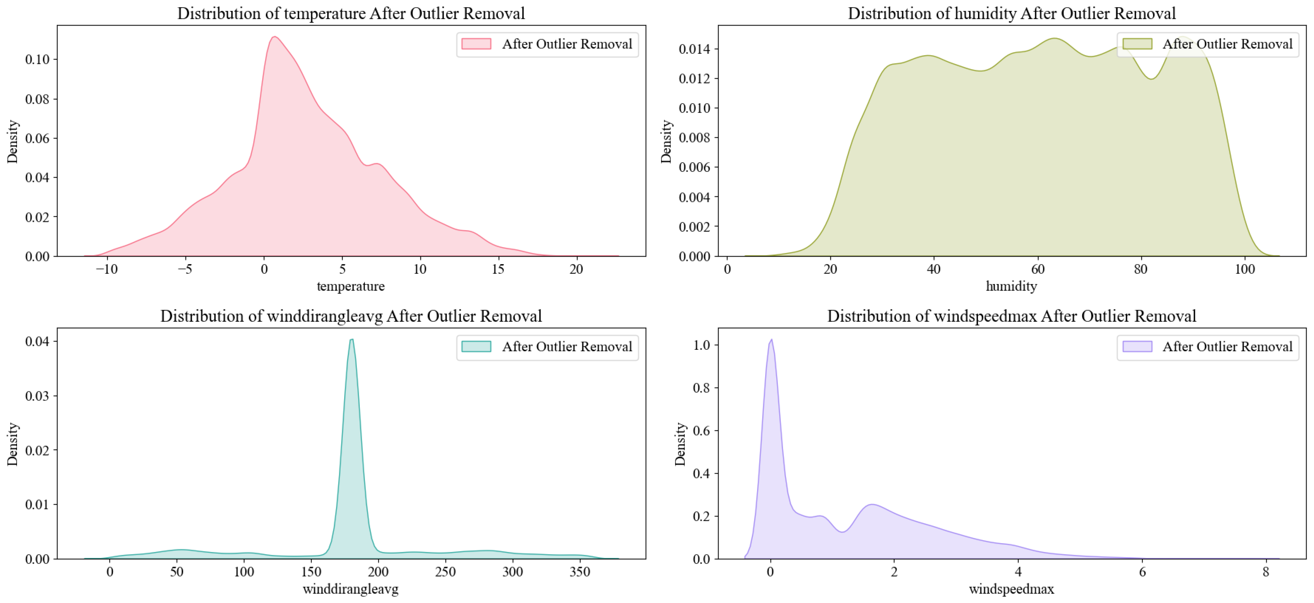
Figure 5 shows the final distribution of sensor values after Isolation Forest-based refinement. The temperature curve becomes bell-shaped, reflecting effective noise suppression. Wind speed anomalies are further reduced while humidity and wind direction remain consistent, indicating their inherent stability and low anomaly prevalence.

To quantify how data cleaning affected statistical properties,

Table 4. Statistical shifts in mean and standard deviation across preprocessing stages.

Feature	Stage	Mean	Std. Dev.
Temperature	Raw	−184.3155	716.8703
	After Thresholding	2.7363	5.0937
	After Isolation Forest	2.7404	4.7631
Humidity	Raw	60.3796	20.9477
	After Thresholding	59.8836	21.8102
	After Isolation Forest	60.5559	21.5633
Wind Direction	Raw	179.4109	60.9069
	After Thresholding	179.2974	67.7044
	After Isolation Forest	179.6466	61.7245
Wind Speed	Raw	1.2507	1.4575
	After Thresholding	1.4088	1.5116
	After Isolation Forest	1.2708	1.3273

reports the mean and variance of each sensor before and after preprocessing. Cleaning produced clear, measurable improvements in statistical stability across the dataset. Temperature showed the largest correction, with an unrealistic raw mean of −184 °C and extremely high variance (std $\approx 716$), which collapsed to realistic environmental values (mean ≈ 2.7 °C, std ≈ 4–5) after threshold filtering and Isolation Forest refinement. Wind speed also exhibited a noticeable reduction in variance following anomaly suppression. In contrast, humidity and wind direction remained statistically consistent across all stages, confirming their low anomaly prevalence. These shifts demonstrate that the proposed preprocessing pipeline effectively removes corrupted samples while preserving genuine environmental dynamics.

3.3. Virtual Sensor Data Generation

To simulate sensor measurements in environments where physical deployment is limited or infeasible, this study utilizes two statistical modeling approaches: BRR and SGPR. These methods generate reliable virtual sensor data by learning from observed values of correlated physical sensors while providing regularization and uncertainty quantification.

3.3.1. Bayesian Ridge Regression

BRR extends Ridge regression by treating the regression weights as random variables with Gaussian priors. This Bayesian formulation allows posterior inference, yielding not only point predictions but also uncertainty estimates.

The likelihood of the observed data is defined as:

$$p(y\mid X,w,\alpha )=\mathcal{N}(y\mid Xw,{\alpha }^{-1}I),$$

(13)

where $X\in {\mathbb{R}}^{N\times M}$ is the feature matrix, $y\in {\mathbb{R}}^N$ the target vector, $w\in {\mathbb{R}}^M$ the regression coefficients, and $\alpha$ the noise precision.

A Gaussian prior is imposed on w:

$$p(w\mid \lambda )=\mathcal{N}(w\mid 0,{\lambda }^{-1}I),$$

(14)

where $\lambda$ is the prior precision (inverse variance) of the weights.

The posterior distribution of w is then:

$$p(w\mid X,y,\alpha ,\lambda )\propto p(y\mid X,w,\alpha )·p(w\mid \lambda ),$$

(15)

which is also Gaussian with:

$$w_{\mathrm{post}}=\alpha \Sigma X^{\top }y,$$

(16)

$$\Sigma ={(\lambda I+\alpha X^{\top }X)}^{-1}.$$

(17)

The predictive distribution for a new input $x_{\ast }$ is:

$$p(y_{\ast }\mid x_{\ast },X,y)=\mathcal{N}\left(y_{\ast }\mid x_{\ast }^{\top }{w}_{\mathrm{post}},{\alpha }^{-1}+x_{\ast }^{\top }\Sigma x_{\ast }\right).$$

(18)

This formulation allows BRR to balance model complexity and noise variance automatically, yielding robust estimates under multicollinearity and limited training samples.

3.3.2. Sparse Gaussian Process Regression

SGPR is a nonparametric Bayesian approach that models functions as distributions over infinite-dimensional feature spaces. It provides both predictions and uncertainty quantification but suffers from a high computational cost $\mathcal{O}\left(N^3\right)$ for N training samples.

Given training data $\mathcal{D}=\{X,y\}$, GPR assumes:

$$f\sim \mathcal{N}(0,K(X,X\left)\right),$$

(19)

where f are latent function values and $K(X,X)$ is the kernel (covariance) matrix, often chosen as the RBF kernel:

$$k(x_p,x_q)={\sigma }_f^{2}exp\left(-{\displaystyle \frac{\parallel x_p-x_q{\parallel }^2}{2{\mathcal{l}}^2}}\right),$$

(20)

with hyperparameters ${\sigma }_f^2$ (signal variance) and ℓ (length scale).

The predictive distribution for a test point $x_{\ast }$ is:

$$p(f_{\ast }\mid x_{\ast },X,y)=\mathcal{N}\left(\mu \left(x_{\ast }\right),{\sigma }^2\left(x_{\ast }\right)\right),$$

(21)

where

$$\mu \left(x_{\ast }\right)=K(x_{\ast },X){\left[K(X,X)+{\sigma }_n^{2}I\right]}^{-1}y,$$

(22)

$${\sigma }^2\left(x_{\ast }\right)=K(x_{\ast },x_{\ast })-K(x_{\ast },X){\left[K(X,X)+{\sigma }_n^{2}I\right]}^{-1}K(X,x_{\ast }).$$

(23)

To improve scalability, Sparse GPR introduces $m\ll N$ inducing points Z with corresponding function values $u=f\left(Z\right)$. The sparse approximation factorizes as:

$$p(f\mid X)\approx \int p(f\mid u,X,Z)p(u\mid Z)du,$$

(24)

which reduces complexity from $\mathcal{O}\left(N^3\right)$ to $\mathcal{O}\left(N{m}^2\right)$.

This approach preserves uncertainty quantification while enabling virtual sensor estimation in real-time or resource-constrained environments.

3.3.3. Statistical Consistency and Cross-Location Validation of Virtual Sensors

A comprehensive validation procedure is applied to assess the fidelity of the virtual sensor outputs with respect to the physical sensor measurements. To evaluate temporal agreement, physical and virtual readings were aligned over shared timestamps, and their correlation was computed using histogram-based Pearson similarity. This verifies that the virtual sensors not only reproduce the statistical properties of the variables but also capture their time-dependent evolution.

To assess data-level consistency, the KS statistic and distribution-shape correlations were computed between the physical and virtual sensor outputs. These metrics quantify how well the virtual sensor preserves the underlying probability distribution of each environmental variable, independent of its forecasting role.

Table 5. Distribution similarity between physical and virtual sensor data using KS statistic and histogram-based correlation.

Variable	KS Statistic	Correlation
BRR Model Results
windspeedmax	0.155953	0.969684
humidity	0.071508	0.413899
winddirangleavg	0.334304	0.095774
temperature	0.058707	0.846754
SGPR Model Results
humidity	0.050252	0.425258
temperature	0.050712	0.864514
winddirangleavg	0.326804	0.123781
windspeedmax	0.151527	0.971990

presents the similarity results for four environmental variables. Temperature and wind speed show strong distributional agreement, as indicated by low KS values and correlation coefficients above 0.84. Humidity and wind direction exhibit moderate similarity due to their greater natural variability and nonlinear behavior yet remain within acceptable consistency boundaries.

In addition to temporal and distributional analysis, cross-location validation was conducted by evaluating the statistical similarity independently across all available sensor channels, treating each as a distinct spatial measurement source. The consistent trends observed across these channels indicate that the virtual sensor models generalize well across varying environmental characteristics. Together, these results confirm that the BRR and SGPR models produce virtual sensor data that is statistically coherent, temporally aligned, and spatially robust.

3.4. Virtual Sensor Data Augmentation

To enhance the diversity and robustness of the virtual sensor dataset generated by statistical models, we employ two deep generative frameworks: the VAE and the CTGAN. These models learn the underlying structure of the data distribution and generate new high-fidelity samples that preserve the statistical and relational properties of the original data. This augmentation improves generalization, mitigates overfitting, and supports downstream deep learning tasks with more comprehensive datasets.

3.4.1. Variational Autoencoder

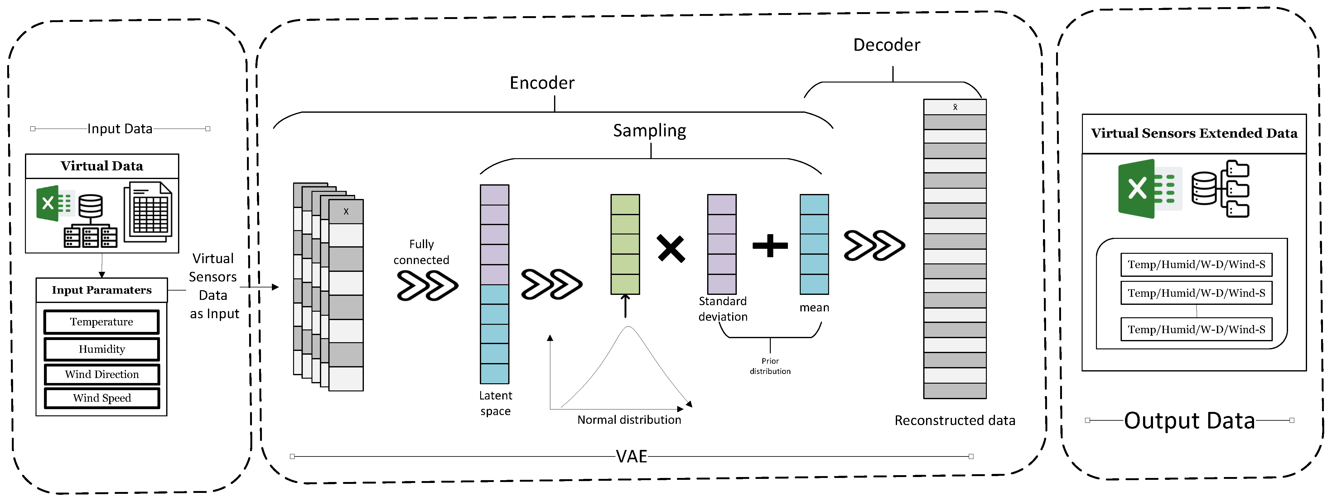
The VAE is a probabilistic deep generative model consisting of an encoder, a latent sampling mechanism, and a decoder, as shown in Figure 6. The encoder compresses input data $x\in {\mathbb{R}}^d$ into parameters of a Gaussian distribution in a latent space:

$$\mu =f_{\mu }\left(x\right),log{\sigma }^2=f_{\sigma }\left(x\right),$$

(25)

where $f_{\mu }$ and $f_{\sigma }$ are neural networks producing the mean and variance.

To enable backpropagation through the stochastic process, the reparameterization trick is applied:

$$z=\mu +\sigma \odot ϵ,ϵ\sim \mathcal{N}(0,I),$$

(26)

where z is the latent vector. The decoder then reconstructs the input from z, producing $\widehat{x}\sim p_{\theta }\left(x\right|z)$.

The VAE objective function is:

$${\mathcal{L}}_{\mathrm{VAE}}(\theta ,\varphi ;x)={\mathbb{E}}_{q_{\varphi }\left(z\right|x)}\left[log{p}_{\theta }\left(x\right|z)\right]-D_{KL}\left(q_{\varphi }\left(z\right|x)\left|\right|p\left(z\right)\right),$$

(27)

where:

-

$q_{\varphi }\left(z\right|x)$ is the encoder’s approximate posterior,

-

$p\left(z\right)=\mathcal{N}(0,I)$ is the prior distribution,

-

$D_{KL}$ is the Kullback–Leibler divergence, enforcing latent regularization.

The first term maximizes the likelihood of reconstructing the input, while the second penalizes divergence from the prior, yielding a structured latent space. This allows the VAE to generate realistic synthetic sensor data while capturing variability across parameters.

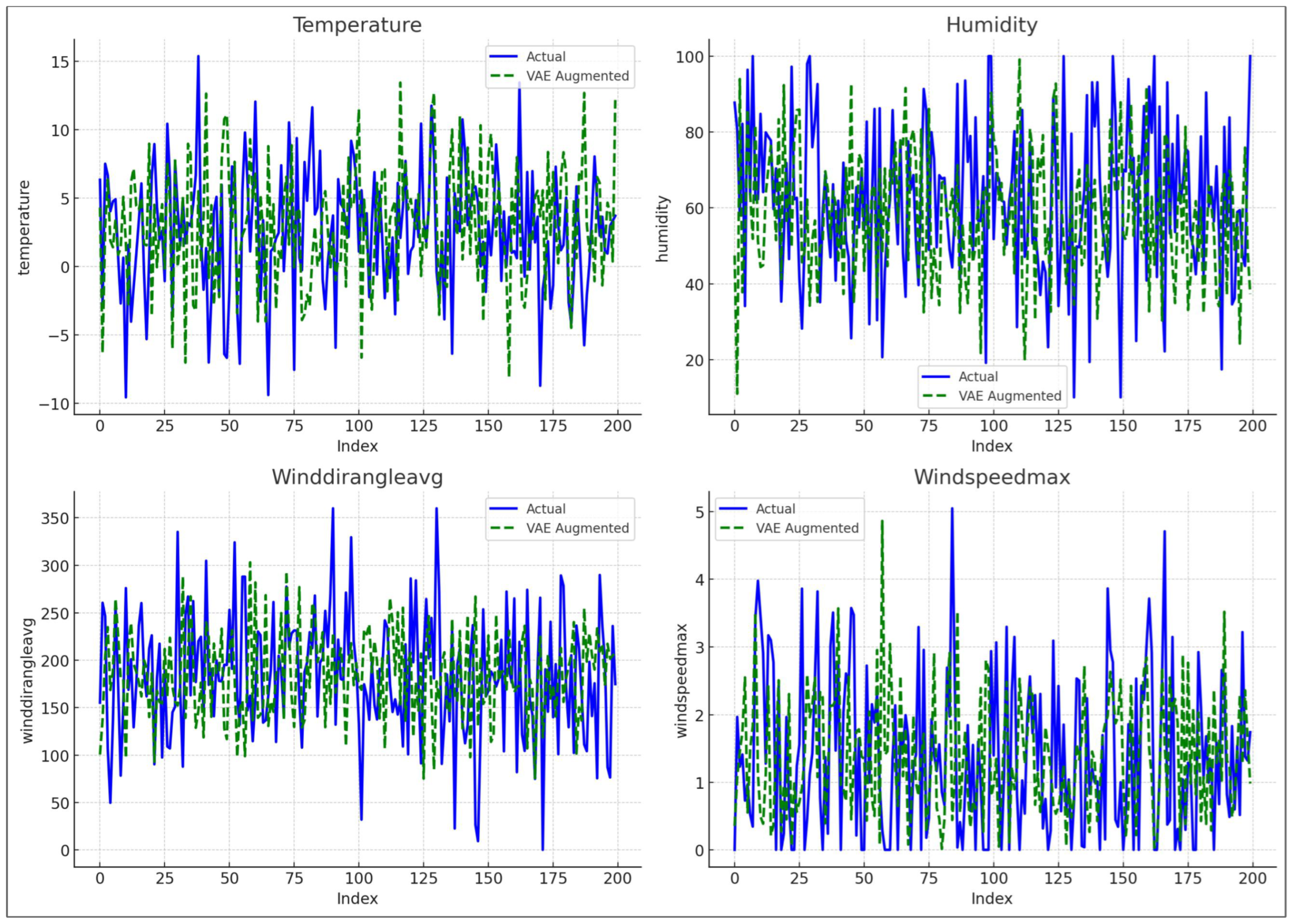
The comparison in Figure 7 demonstrates that the VAE-augmented data maintains close alignment with the actual sensor observations across all four environmental features. The overlapping line patterns confirm that the generative process does not distort the underlying structure, while the subtle deviations reflect the model’s ability to enrich variability. This balance between fidelity and diversity ensures that the augmented dataset can support downstream learning tasks by providing additional training samples that mimic realistic fluctuations. Consequently, VAE proves effective in producing high-quality synthetic data, particularly in contexts where physical sensor availability is constrained.

3.4.2. Conditional Tabular GAN

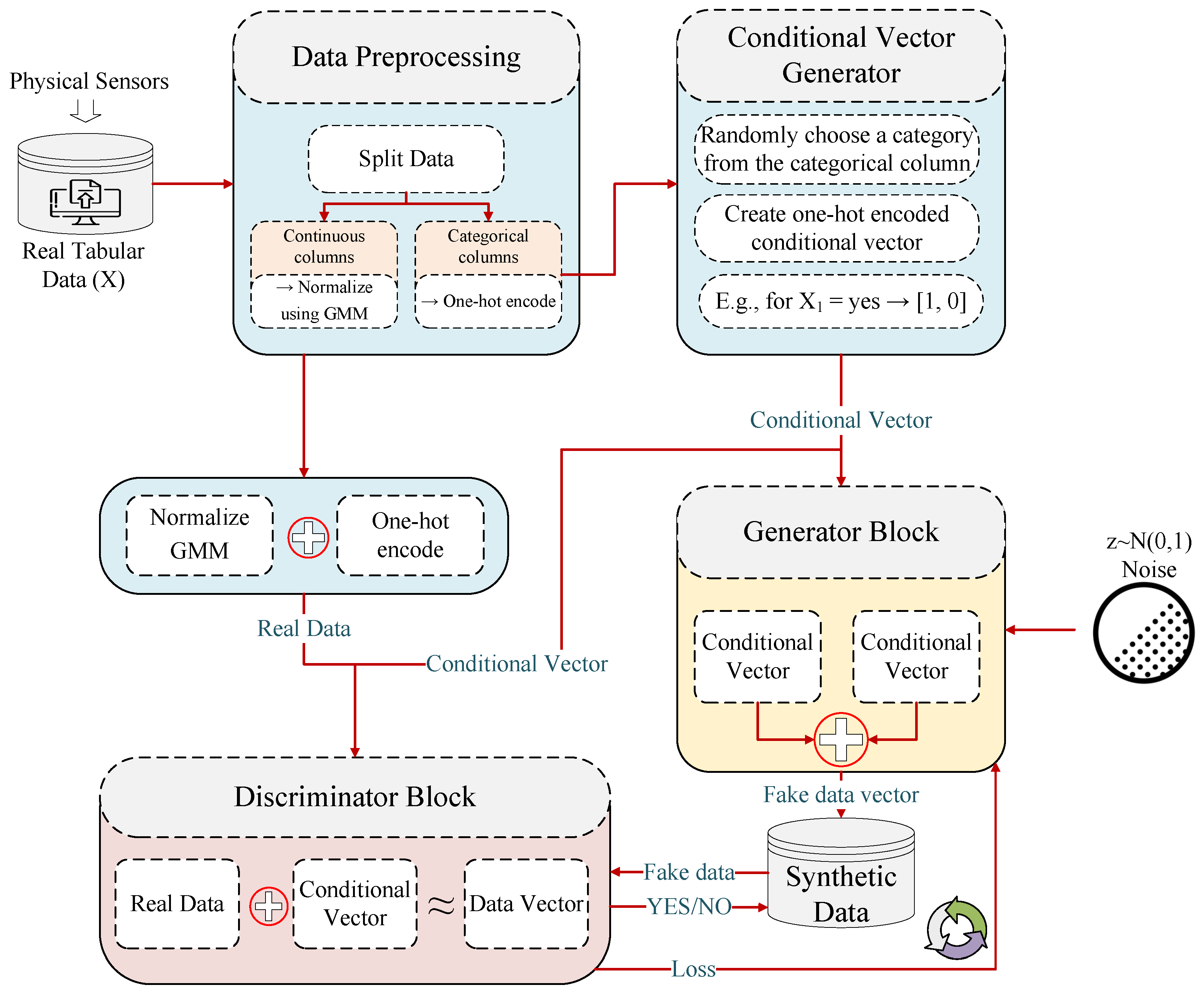
The CTGAN is specifically designed for generating synthetic tabular data with both continuous and categorical variables, as illustrated in Figure 8. The preprocessing step normalizes continuous features using Gaussian Mixture Models (GMMs) to capture multi-modal distributions and applies one-hot encoding to categorical variables. A conditional vector $\mathbf{c}$ is generated to enforce category-level conditioning during synthesis.

The generator G takes as input a noise vector $\mathbf{z}\sim \mathcal{N}(0,I)$ and a conditional vector $\mathbf{c}$, producing synthetic samples:

$$\tilde{\mathbf{x}}=G(\mathbf{z},\mathbf{c}).$$

(28)

The discriminator D receives either real data $\mathbf{x}$ or generated data $\tilde{\mathbf{x}}$, along with the same conditional vector $\mathbf{c}$, and outputs a probability that the input is real. The adversarial training objective is:

$$\underset{G}{min}\underset{D}{max}{\mathbb{E}}_{\mathbf{x}\sim p_{\mathrm{data}}}\left[logD(\mathbf{x},\mathbf{c})\right]+{\mathbb{E}}_{\mathbf{z}\sim p\left(\mathbf{z}\right)}\left[log\left(1-D\left(G\right(\mathbf{z},\mathbf{c}),\mathbf{c})\right)\right].$$

(29)

This objective ensures that:

-

the generator learns to create realistic tabular data conditioned on specific categories,

-

the discriminator improves its ability to detect synthetic vs. real data.

By integrating GMM normalization for continuous features and conditional sampling for categorical ones, CTGAN effectively models the complex mixed-type distributions present in environmental sensor data.

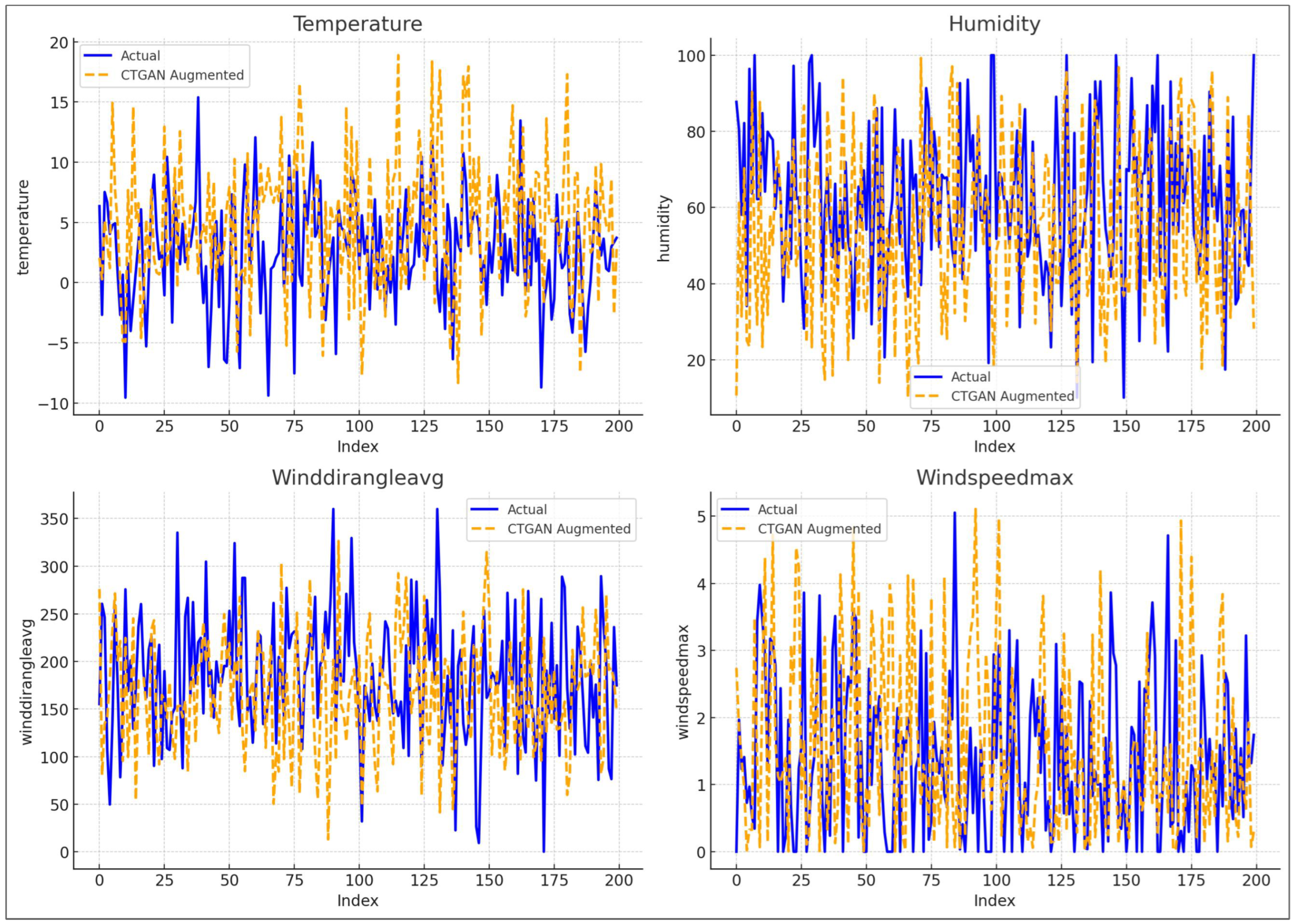
As shown in Figure 9, CTGAN-generated samples closely follow the temporal patterns of the actual sensor data, demonstrating strong alignment across all four features. The synthetic data introduces modest fluctuations and extended variability compared to the original series, indicating its ability to capture more complex and nuanced structures. This enhancement improves the richness of the dataset and reduces the risk of overfitting in downstream models. By generating realistic yet diverse synthetic data, CTGAN provides an effective augmentation strategy for virtual sensing, particularly when working with mixed-type environmental datasets.

3.4.3. Quantitative Assessment of Trend and Distribution Preservation

To address the need for a measurable evaluation of the similarity between the actual and augmented datasets, we computed two quantitative metrics: the Kolmogorov–Smirnov (KS) statistic and the Pearson correlation coefficient. These metrics provide complementary insights into how well the generative models (VAE and CTGAN) preserve the statistical and temporal properties of the physical sensor data.

The KS statistic measures the maximum deviation between the empirical cumulative distribution functions of two datasets. Lower KS values indicate that the augmented data follows the same underlying distribution as the real sensor observations. Pearson correlation, on the other hand, quantifies the linear association between the actual and augmented time series, thereby capturing trend and temporal pattern similarity.

Table 6. Quantitative comparison between actual and augmented datasets using KS statistic and Pearson correlation. Lower KS and higher correlation indicate better preservation of original data characteristics.

Variable	KS_CTGAN	KS_VAE	Corr_CTGAN	Corr_VAE
Temperature	0.0950	0.0490	0.8722	0.8996
Humidity	0.0360	0.0510	0.6439	0.6381
Wind Direction	0.1045	0.0475	0.8785	0.9201
Wind Speed	0.1765	0.1765	0.5265	0.2983

Note: Best-performing values for each variable are indicated bold style.

summarizes the results for the four environmental variables. VAE augmentation demonstrates notably lower KS distances for temperature and wind direction, indicating close distributional alignment with the actual data. These variables also exhibit strong temporal similarity, with correlations above 0.89. CTGAN achieves comparable or better performance for humidity and wind speed, reflecting its ability to model higher-variance and more stochastic variables. Together, these quantitative results confirm that both generative models preserve essential characteristics of the original dataset, with VAE showing overall stronger alignment to the physical sensor behavior.

3.5. Learning Models

To evaluate the predictive performance of the proposed VSG-SGL framework, two advanced recurrent neural network (RNN) architectures are utilized: BiLSTM and BiGRU. Both models are designed for sequential data and are effective in capturing temporal dependencies across time steps, which is essential for univariate and multivariate time-series forecasting of environmental variables such as temperature, humidity, wind direction, and wind speed. By comparing predictions generated from physical and virtual sensor data, these models enable a comprehensive assessment of the framework’s reliability and efficiency.

3.5.1. Bidirectional Long Short-Term Memory (BiLSTM)

The LSTM architecture extends traditional RNNs by introducing gating mechanisms that mitigate the vanishing gradient problem. Each LSTM cell maintains both a memory state $c_t$ and a hidden state $h_t$, updated at each time step t as:

$$\begin{array}{cc}\hfill f_t& =\sigma (W_f[h_{t-1},x_t]+b_f),\hfill \end{array}$$

(30)

$$\begin{array}{cc}\hfill i_t& =\sigma (W_i[h_{t-1},x_t]+b_i),\hfill \end{array}$$

(31)

$$\begin{array}{cc}\hfill {\tilde{c}}_t& =tanh(W_c[h_{t-1},x_t]+b_c),\hfill \end{array}$$

(32)

$$\begin{array}{cc}\hfill c_t& =f_t\odot c_{t-1}+i_t\odot {\tilde{c}}_t,\hfill \end{array}$$

(33)

$$\begin{array}{cc}\hfill o_t& =\sigma (W_o[h_{t-1},x_t]+b_o),\hfill \end{array}$$

(34)

$$\begin{array}{cc}\hfill h_t& =o_t\odot tanh\left(c_t\right),\hfill \end{array}$$

(35)

where $x_t\in {\mathbb{R}}^d$ is the input vector, $\sigma (·)$ is the sigmoid activation, and ⊙ denotes element-wise multiplication. The gates $f_t$, $i_t$, and $o_t$ correspond to forget, input, and output operations, respectively.

In BiLSTM, two LSTM layers process the sequence in opposite directions: forward ($\overrightarrow{h_t}$) and backward ($\overleftarrow{h_t}$). The final hidden state is obtained by concatenation:

$$h_t^{\mathrm{BiLSTM}}=[\overrightarrow{h_t};\overleftarrow{h_t}],$$

(36)

which captures both past and future temporal dependencies. For forecasting, the BiLSTM outputs ${\widehat{y}}_t$ are compared to ground-truth values $y_t$ using a regression loss (e.g., Mean Squared Error):

$${\mathcal{L}}_{\mathrm{MSE}}={\displaystyle \frac{1}{N}}\sum _{t=1}^N{\left(y_t-{\widehat{y}}_t\right)}^2.$$

(37)

This bidirectional design is advantageous in environmental monitoring, where sensor readings are often influenced by long-range contextual factors and cyclical patterns.

The training process of the BiLSTM model follows a structured sequence of forward and backward passes, where hidden and cell states are updated at each timestep using gating mechanisms. Algorithm 2 outlines the complete procedure, including initialization, forward and backward propagation, prediction, loss computation, and parameter updates.

Algorithm 2 Training Procedure of BiLSTM for Virtual Sensor Forecasting

3.5.2. Bidirectional Gated Recurrent Unit (BiGRU)

The GRU simplifies LSTM by merging the forget and input gates into a single update gate and removing the explicit memory state $c_t$. Its lower computational complexity makes it suitable for large-scale sensor forecasting while preserving accuracy. The GRU cell is governed by:

$$\begin{array}{cc}\hfill z_t& =\sigma (W_z[h_{t-1},x_t]+b_z),\hfill \end{array}$$

(38)

$$\begin{array}{cc}\hfill r_t& =\sigma (W_r[h_{t-1},x_t]+b_r),\hfill \end{array}$$

(39)

$$\begin{array}{cc}\hfill {\tilde{h}}_t& =tanh(W_h[r_t\odot h_{t-1},x_t]+b_h),\hfill \end{array}$$

(40)

$$\begin{array}{cc}\hfill h_t& =(1-z_t)\odot h_{t-1}+z_t\odot {\tilde{h}}_t,\hfill \end{array}$$

(41)

where $z_t$ is the update gate regulating the balance between past and new information, $r_t$ is the reset gate controlling memory reset, and ${\tilde{h}}_t$ is the candidate hidden state.

In BiGRU, the forward and backward hidden states are concatenated:

$$h_t^{\mathrm{BiGRU}}=[\overrightarrow{h_t};\overleftarrow{h_t}],$$

(42)

providing temporal context from both directions. Similar to BiLSTM, BiGRU is trained using a regression loss (e.g., MSE), while additional metrics such as MAE and RMSE, already defined in Section 4, are used for performance assessment.

3.5.3. Training Objective

Both BiLSTM and BiGRU are trained to minimize the predictive error between actual and estimated environmental variables. Given the sequential nature of sensor data, the models optimize the following objective:

$$\underset{\Theta }{min}{\mathbb{E}}_{(x_t,y_t)\sim \mathcal{D}}\left[\mathcal{l}\left(f_{\Theta }\left(x_{1:t}\right),y_t\right)\right],$$

(43)

where $f_{\Theta }$ denotes the neural model parameterized by weights $\Theta$, $\mathcal{l}(·)$ is the loss function (e.g., MSE), and $\mathcal{D}$ represents the training dataset. Optimization is performed using stochastic gradient descent with Adam, updating parameters iteratively as:

$$\Theta \leftarrow \Theta -\eta ·{\nabla }_{\Theta }\mathcal{L},$$

(44)

with learning rate $\eta$ and gradient ${\nabla }_{\Theta }\mathcal{L}$.

The BiGRU model streamlines the learning process by employing reset and update gates, eliminating the explicit memory cell used in LSTMs. Its training procedure is summarized in Algorithm 3, which details the forward and backward passes, concatenation of hidden states, prediction, loss evaluation, and optimization of parameters.

Algorithm 3 Training Procedure of BiGRU for Virtual Sensor Forecasting

4. Evaluation Metrics

To quantitatively assess the predictive accuracy of the proposed framework, three complementary regression metrics are employed: MSE, MAE, and RMSE. Together, these metrics capture different dimensions of model performance, including sensitivity to large deviations, overall error magnitude, and interpretability.

The MSE measures the average of the squared differences between predicted and actual values:

$$\mathrm{MSE}={\displaystyle \frac{1}{n}}\sum _{i=1}^n{(y_i-{\widehat{y}}_i)}^2.$$

(45)

Due to the squaring operation, MSE disproportionately penalizes larger errors, making it a valuable indicator of how the model responds to abrupt fluctuations or extreme event conditions frequently encountered in environmental sensing.

The MAE computes the mean magnitude of prediction errors:

$$\mathrm{MAE}={\displaystyle \frac{1}{n}}\sum _{i=1}^n\left|y_i-{\widehat{y}}_i\right|.$$

(46)

Unlike MSE, MAE weights all deviations linearly and is therefore more robust to outliers. It provides a stable assessment of the model’s average predictive deviation across all samples, making it particularly useful for variables with heterogeneous noise characteristics.

The RMSE is defined as the square root of MSE:

$$\mathrm{RMSE}=\sqrt{{\displaystyle \frac{1}{n}}\sum _{i=1}^n{(y_i-{\widehat{y}}_i)}^2}.$$

(47)

RMSE expresses the error in the same scale and unit as the target variable, offering an intuitive interpretation of the expected prediction error. While RMSE is mathematically related to MSE, it serves a distinct purpose: whereas MSE highlights the model’s sensitivity to large deviations, RMSE provides a directly interpretable estimate of the typical error magnitude. Reporting both enables a more nuanced understanding of model behavior under varying levels of variability and noise.

By jointly analyzing MAE, MSE, and RMSE, the evaluation provides a balanced and comprehensive view of the model’s predictive performance across diverse environmental sensor variables.

5. Experimental Results

This section presents a comprehensive evaluation of the proposed VSG-SGL framework for generating and augmenting virtual sensor data. The experiments aim to assess the performance of virtual sensors derived via statistical models (BBR and SGPR) and further enhanced through data augmentation techniques using VAE and CTGAN. Two deep learning models, BiLSTM and BiGRU, are employed to evaluate the predictive capability of both physical and virtual sensor data, using three error metrics: MAE, MSE, and RMSE.

5.1. Development Environment for Proposed Approach

The system configuration and software stack used for implementation and experimentation are summarized in

Table 7. Development Environment.

S.No	Component	Description
1	Operating System	Windows 11 for PC Server
2	RAM	94 GB
3	Processor	12th Gen Intel® CoreTM i9-12900K CPU @ 3.20 GHz
4	Programming Language	Python
5	IDE	PyCharm
6	Data Storage	MS Excel
7	Core Libraries	Pandas, Scikit-learn, Keras, TensorFlow, Seaborn, Matplotlib, etc.

.

5.2. Results on Physical Sensor Data

Table 8. Performance of learning models on physical sensor data.

Sensor	BiLSTM			BiGRU
	MAE	MSE	RMSE	MAE	MSE	RMSE
Temperature	0.0552	0.0057	0.0757	0.0686	0.0083	0.0912
Humidity	0.0732	0.0112	0.1061	0.0855	0.0134	0.1157
Wind Direction	0.1518	0.0476	0.2182	0.1520	0.0476	0.2182
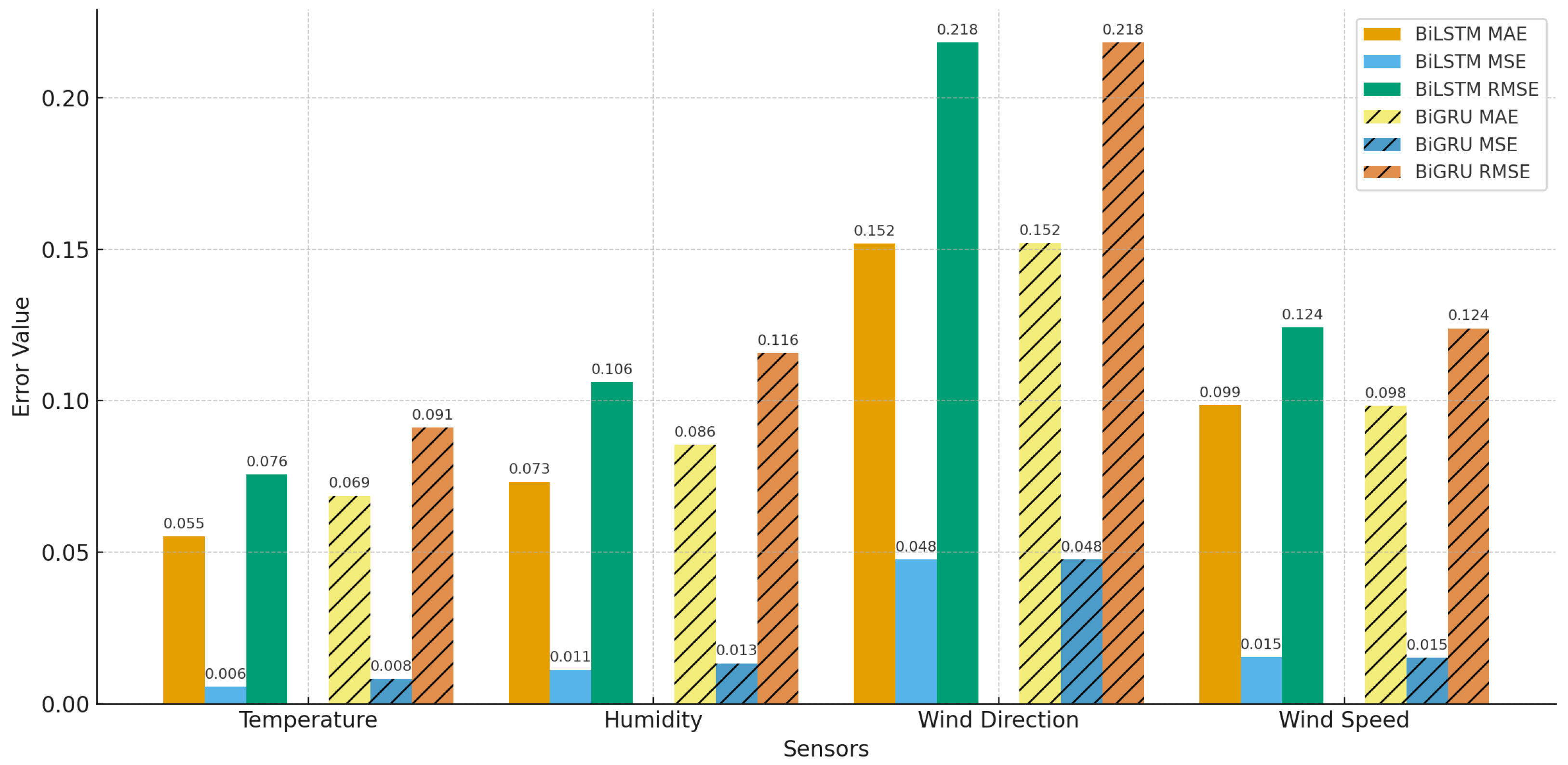
Wind Speed	0.0985	0.0154	0.1242	0.0984	0.0153	0.1239

summarizes the performance of the BiLSTM and BiGRU models on real-world physical sensor data. The BiLSTM consistently yields lower error across all sensor variables compared to BiGRU. The Temperature sensor shows the lowest prediction error, suggesting its temporal patterns are easier to model. Conversely, Wind Direction and Wind Speed sensors exhibit relatively higher errors, likely due to their more complex or stochastic behavior.

The bar graph in Figure 10 presents a normalized comparison of the BiLSTM and BiGRU error metrics (MAE, MSE, RMSE) across the four physical sensor variables. Since each variable operates on a different scale, all error values have been normalized to the range [0, 1] to ensure unit-independent interpretation. The results show that BiLSTM consistently achieves lower normalized error values than BiGRU, particularly for Temperature and Humidity, where the temporal patterns are smoother and more predictable. In contrast, Wind Direction and Wind Speed exhibit higher error magnitudes for both models, reflecting the inherently stochastic, nonlinear, and rapidly fluctuating behavior of these variables. Overall, the visualization highlights the superior predictive capability of BiLSTM while emphasizing the additional modeling challenges associated with directional and high-variability environmental data.

5.3. Results with BRR and Data Augmentation

Table 9. Performance of learning models on virtual sensors (Bayesian Ridge, CTGAN, VAE).

Sensor	BiLSTM			BiGRU
	MAE	MSE	RMSE	MAE	MSE	RMSE
BRR
Temperature	0.1194	0.0229	0.1514	0.1209	0.0235	0.1532
Humidity	0.1880	0.0525	0.2290	0.1879	0.0529	0.2301
Wind Direction	0.1483	0.0339	0.1842	0.1491	0.0342	0.1849
Wind Speed Max	0.1711	0.0437	0.2091	0.1709	0.0434	0.2083
Bayesian+CTGAN
Temperature	0.1919	0.0578	0.2404	0.1967	0.0604	0.2457
Humidity	0.1805	0.0495	0.2224	0.1856	0.0527	0.2300
Wind Direction	0.1847	0.0529	0.2301	0.1786	0.0499	0.2235
Wind Speed Max	0.1419	0.0369	0.1922	0.1422	0.0364	0.1908
Bayesian+VAE
Temperature	0.1371	0.0292	0.1708	0.1383	0.0294	0.1715
Humidity	0.1730	0.0440	0.2097	0.1745	0.0452	0.2126
Wind Direction	0.1402	0.0298	0.1726	0.1936	0.0546	0.2337
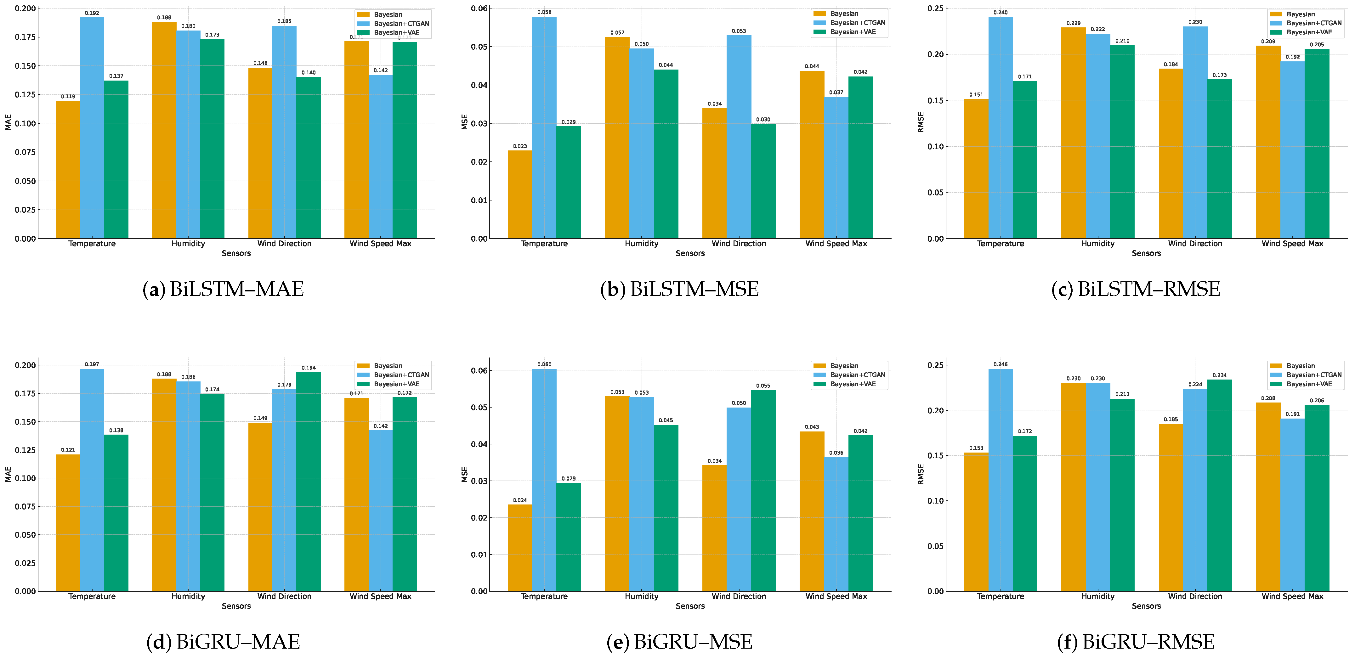
Wind Speed Max	0.1705	0.0422	0.2055	0.1715	0.0423	0.2057

reports the performance of virtual sensor data generated using BRR, followed by augmentation with CTGAN and VAE. The following observations are made:

• BRR yields reasonably close performance to the real sensor data, with slightly higher error values.
• VAE-augmented data consistently improves model accuracy, reducing MAE and RMSE, especially for temperature and Wind Direction.
• CTGAN-based augmentation introduces variability and often leads to performance degradation, particularly for wind speed and humidity.

The BiLSTM model outperforms BiGRU in most settings when using Bayesian Ridge-generated data.

Figure 11 presents the consolidated performance of BiLSTM (top row) and BiGRU (bottom row) across MAE, MSE, and RMSE for BRR and its augmented variants. The BiLSTM model consistently outperforms BiGRU, showing lower error values across most sensors. VAE augmentation yields the most notable improvements, particularly for Temperature and Wind Direction, where it reduces both MAE and RMSE compared to baseline Bayesian Ridge. Conversely, CTGAN augmentation introduces higher variability, often degrading performance for Humidity and Wind Speed. These results emphasize that VAE provides a stable path for enhancing virtual sensor quality, while BiLSTM remains the more reliable model for capturing temporal dependencies in environmental data.

5.4. Results with Sparse GPR and Data Augmentation

Table 10. Performance of learning models on virtual sensors (Sparse GPR, CTGAN, VAE).

Sensor	BiLSTM			BiGRU
	MAE	MSE	RMSE	MAE	MSE	RMSE
Sparse GPR
Temperature	0.1283	0.0267	0.1635	0.1284	0.0269	0.1640
Humidity	0.1857	0.0519	0.2277	0.1858	0.0519	0.2278
Wind Direction	0.1346	0.0290	0.1703	0.1372	0.0300	0.1733
Wind Speed Max	0.1848	0.0493	0.2220	0.1847	0.0492	0.2218
Sparse GPR+CTGAN
Temperature	0.1801	0.0523	0.2287	0.1884	0.0583	0.2415
Humidity	0.1970	0.0567	0.2381	0.2018	0.0628	0.2505
Wind Direction	0.2096	0.0666	0.2570	0.1850	0.0510	0.2259
Wind Speed Max	0.2117	0.0714	0.2671	0.2082	0.0673	0.2594
Sparse GPR+VAE
Temperature	0.1330	0.0287	0.1695	0.1321	0.0283	0.1683
Humidity	0.1748	0.0459	0.2144	0.1877	0.0529	0.2299
Wind Direction	0.1429	0.0302	0.1739	0.1529	0.0338	0.1839
Wind Speed Max	0.1604	0.0396	0.1989	0.1608	0.0399	0.1998

reports experimental results using SGPR and its augmentation using CTGAN and VAE. Key insights include:

• Sparse GPR+VAE yields the most balanced and robust results across all sensors, especially for Temperature and Wind Direction.
• CTGAN augmentation again results in unstable performance, particularly for Wind Speed.

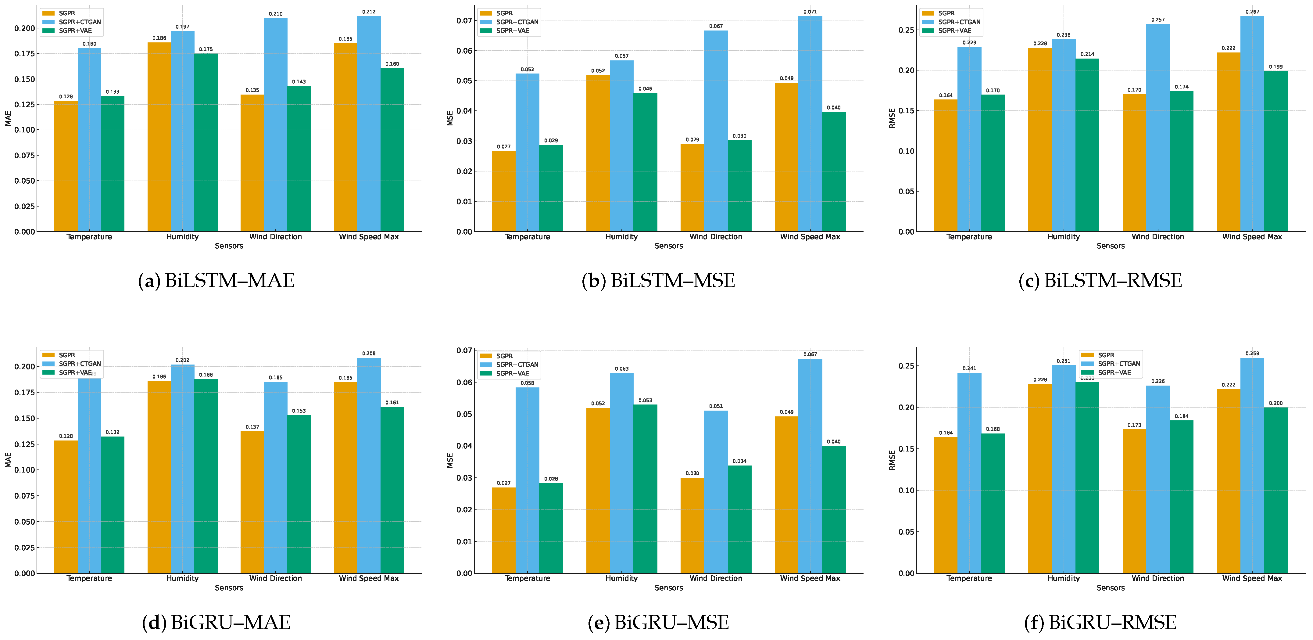
Figure 12 illustrates the comparative performance of BiLSTM (top row) and BiGRU (bottom row) models under Sparse GPR and its augmented variants. The baseline SGPR demonstrates moderate predictive ability, but augmentation with VAE improves overall accuracy, particularly for Temperature and Wind Direction, with reductions in MAE and RMSE. In contrast, CTGAN augmentation leads to higher errors across all metrics, most prominently for Wind Speed and Humidity, indicating instability in capturing temporal dynamics. BiLSTM again outperforms BiGRU, highlighting its stronger capacity for modeling sequential dependencies when learning from augmented virtual sensor data.

5.5. Comparison Summary

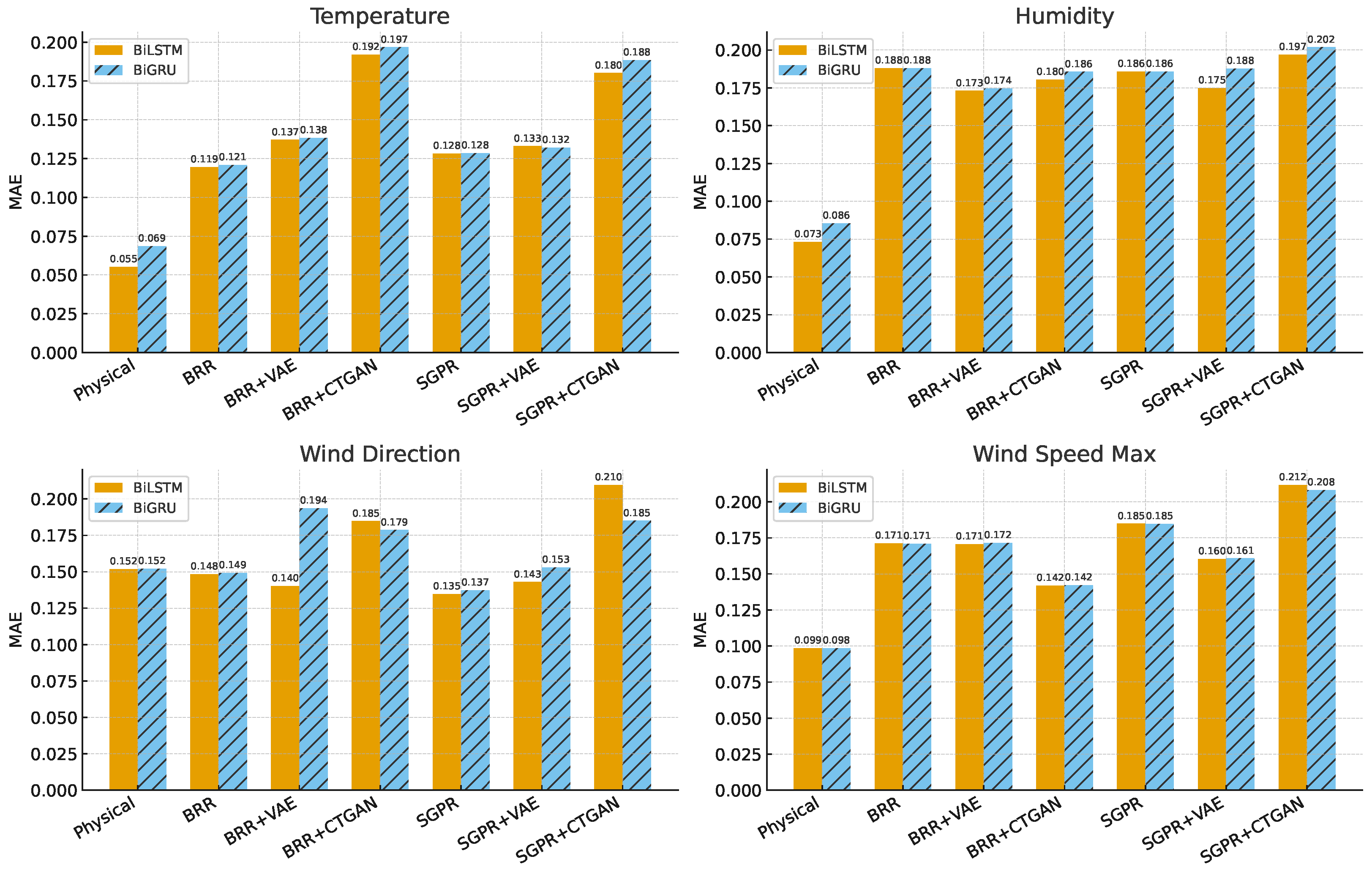
Figure 13 consolidates MAE results over all data-generation scenarios for each sensor. Three consistent trends emerge. First, VAE-augmented virtual sensors (both BRR+VAE and SGPR+VAE) generally reduce error relative to the unaugmented baselines, with the strongest gains for Temperature and Wind Direction. Second, CTGAN augmentation is less reliable: errors typically increase, most notably for Humidity and Wind Speed, indicating instability for these variables. Third, BiLSTM outperforms BiGRU in most settings, though their performance is close on the simpler Temperature series. Taken together, these results support the use of VAE-augmented virtual sensors as robust substitutes when physical sensing is sparse or unavailable, while favoring BiLSTM for downstream forecasting.

6. Ablation Study

To better understand the contribution of each component in the proposed VSG-SGL framework, we conducted a comprehensive ablation study. This study aims to evaluate the individual and combined impact of virtual data generation methods, data augmentation techniques, and deep learning models on prediction performance. By selectively excluding or including each module, we assess their influence on model accuracy.

The ablation results in

Table 11. Ablation study results (MAE).

Setup	Temperature	Humidity	Wind Direction	Wind Speed
A1: Physical Only	0.0552	0.0732	0.1518	0.0985
A2: +Bayesian	0.1194	0.1880	0.1483	0.1711
A3: +Sparse GPR	0.1283	0.1857	0.1346	0.1848
A4: A2+CTGAN	0.1919	0.1805	0.1847	0.1419
A5: A2+VAE	0.1371	0.1730	0.1402	0.1705
A6: A3+CTGAN	0.1801	0.1970	0.2096	0.2117
A7: A3+VAE	0.1330	0.1748	0.1429	0.1604

clearly highlight the individual contributions of each module. While the Bayesian-generated data (A2) slightly elevates the MAE values, it provides diversity to the training data and lays a foundation for more advanced augmentation strategies. Sparse GPR (A3) contributes to improved wind direction prediction and offers a promising direction for enhancing model robustness. The combination of Sparse GPR with CTGAN (A4, A6) increases variability in the dataset, providing valuable insight into the model’s sensitivity to data distribution. Notably, the Sparse GPR+VAE configuration (A7) achieves the lowest MAE across all sensors, demonstrating that this pairing yields the most effective and reliable augmentation, and confirming its strong potential for improving predictive performance.

7. Conclusions

This study presented VSG-SGL, a unified and systematically validated framework for virtual sensor generation that integrates regression-based modeling (BRR, SGPR) with deep generative augmentation (VAE, CTGAN). A comprehensive evaluation across physical sensor data and multiple virtual-sensor configurations demonstrated that VAE provides the most robust augmentation strategy. For temperature, generative augmentation does not yield improvements but maintains accuracy relative to the baseline regression models (BRR RMSE: 0.1514 → 0.1708; SGPR RMSE: 0.1635 → 0.1695), indicating that the underlying temperature dynamics are already well captured without additional generative refinements. In contrast, humidity and wind-dependent variables benefit more clearly from VAE augmentation. Humidity MAE decreases from 0.1880 to 0.1730 (BRR) and from 0.1857 to 0.1748 (SGPR), while SGPR-based wind speed MAE improves from 0.1848 to 0.1604. Wind direction also shows enhancement under BRR+VAE (MAE: 0.1483 → 0.1402), though performance remains comparable under SGPR+VAE. CTGAN consistently introduces greater variability and degraded accuracy, particularly for humidity and wind speed.

Collectively, these results confirm that VAE-enhanced virtual sensors can emulate or surpass the performance of regression-only models for several key environmental variables, while preserving stability for others such as temperature. The proposed VSG-SGL framework, therefore, provides a scalable, data-efficient, and cost-effective pathway for environmental sensing in regions where physical sensor deployment is limited. Future extensions will focus on multi-modal virtual sensing, adaptive generative modeling, and federated learning to support distributed, privacy-preserving virtual sensor networks.

References

- Sani, S.A. Drawbacks of traditional environmental monitoring systems. TMP Univers. J. Res. Rev. Arch. 2023, 2, 70–75. [Google Scholar] [CrossRef]
- Willard, J.; Jia, X.; Xu, S.; Steinbach, M.; Kumar, V. Integrating physics-based modeling with machine learning: A survey. arXiv 2020, arXiv:2003.04919. [Google Scholar]
- Girin, L.; Leglaive, S.; Bie, X.; Diard, J.; Hueber, T.; Alameda-Pineda, X. Dynamical variational autoencoders: A comprehensive review. arXiv 2020, arXiv:2008.12595. [Google Scholar]
- Xu, L. Synthesizing Tabular Data Using Conditional GAN. Ph.D. Thesis, Massachusetts Institute of Technology, Cambridge, MA, USA, 2020. [Google Scholar]
- Hoang, T.N.; Hoang, Q.M.; Low, B.K.H. A unifying framework of anytime Sparse Gaussian Process Regression models with stochastic variational inference for big data. In Proceedings of the International Conference on Machine Learning, PMLR, Lille, France, 6–11 July 2015; pp. 569–578. [Google Scholar]
- da Silva, F.A.; Viana, A.P.; Correa, C.C.G.; Santos, E.A.; de Oliveira, J.A.V.S.; Andrade, J.D.G.; Ribeiro, R.M.; Glória, L.S. Bayesian ridge regression shows the best fit for SSR markers in Psidium guajava among Bayesian models. Sci. Rep. 2021, 11, 13639. [Google Scholar] [CrossRef] [PubMed]
- Stavropoulos, G.; Violos, J.; Tsanakas, S.; Leivadeas, A. Enabling artificial intelligent virtual sensors in an IoT environment. Sensors 2023, 23, 1328. [Google Scholar] [CrossRef]
- Wu, R.C. Development of an Intelligent Virtualization Platform Key Metrics Monitoring System: Collaborative Implementation with Self-Training and Bagging Algorithm. Mob. Netw. Appl. 2024, 29, 905–921. [Google Scholar] [CrossRef]
- Zhu, Q.X.; Hou, K.R.; Chen, Z.S.; Gao, Z.S.; Xu, Y.; He, Y.L. Novel virtual sample generation using conditional GAN for developing soft sensor with small data. Eng. Appl. Artif. Intell. 2021, 106, 104497. [Google Scholar] [CrossRef]
- Paepae, T.; Bokoro, P.N.; Kyamakya, K. Data augmentation for a virtual-sensor-based nitrogen and phosphorus monitoring. Sensors 2023, 23, 1061. [Google Scholar] [CrossRef]
- Planche, B.; Singh, R.V. Physics-based differentiable depth sensor simulation. In Proceedings of the IEEE/CVF International Conference on Computer Vision, Montreal, QC, Canada, 10–17 October 2021; pp. 14387–14397. [Google Scholar]
- Kullaa, J. Damage detection and localization under variable environmental conditions using compressed and reconstructed bayesian virtual sensor data. Sensors 2021, 22, 306. [Google Scholar] [CrossRef]
- Zhongda, S. AI-Enhanced Human-Machine Interfaces Using Integrated Multi-Modal Sensing and Haptic-Augmented Functions for Digital Twin and Metaverse. Ph.D. Thesis, National University of Singapore, Singapore, 2023. [Google Scholar]
- Almutairi, R.; Bergami, G.; Morgan, G. Advancements and challenges in IoT simulators: A comprehensive review. Sensors 2024, 24, 1511. [Google Scholar] [CrossRef]
- Ergan, S.; Zou, Z.; Bernardes, S.D.; Zuo, F.; Ozbay, K. Developing an integrated platform to enable hardware-in-the-loop for synchronous VR, traffic simulation and sensor interactions. Adv. Eng. Inform. 2022, 51, 101476. [Google Scholar] [CrossRef]
- Mihai, S.; Yaqoob, M.; Hung, D.V.; Davis, W.; Towakel, P.; Raza, M.; Karamanoglu, M.; Barn, B.; Shetve, D.; Prasad, R.V.; et al. Digital twins: A survey on enabling technologies, challenges, trends and future prospects. IEEE Commun. Surv. Tutor. 2022, 24, 2255–2291. [Google Scholar] [CrossRef]
- Zhang, Y.; Liu, J.; Shen, W. A review of ensemble learning algorithms used in remote sensing applications. Appl. Sci. 2022, 12, 8654. [Google Scholar] [CrossRef]
- Chander, B. Artificial Neural Networks and Support Vector Machine for IoT. In Artificial Intelligence-Based Internet of Things Systems; Springer: Cham, Switzerland, 2022; pp. 77–103. [Google Scholar]
- Tajnafoi, G.; Arcucci, R.; Mottet, L.; Vouriot, C.; Molina-Solana, M.; Pain, C.; Guo, Y.K. Variational gaussian process for optimal sensor placement. Appl. Math. 2021, 66, 287–317. [Google Scholar] [CrossRef]
- Xu, L.; Skoularidou, M.; Cuesta-Infante, A.; Veeramachaneni, K. Modeling tabular data using conditional gan. In Proceedings of the Advances in Neural Information Processing Systems 32, Vancouver, BC, Canada, 8–14 December 2019. [Google Scholar]
- Wang, Y.; Yan, P. RegGAN: A virtual sample generative network for developing soft sensors with small data. ACS Omega 2024, 9, 5954–5965. [Google Scholar] [CrossRef]
- Xu, Y.; Zhu, Q.X.; Ke, W.; He, Y.L.; Zhang, M.Q.; Xu, Y. Virtual sample generation for soft-sensing in small sample scenarios using glow-embedded variational autoencoder. Comput. Chem. Eng. 2025, 193, 108925. [Google Scholar] [CrossRef]
- Bournet, P.E.; Rojano, F. Advances of Computational Fluid Dynamics (CFD) applications in agricultural building modelling: Research, applications and challenges. Comput. Electron. Agric. 2022, 201, 107277. [Google Scholar] [CrossRef]
- Ahmed, B. Mathematical Modeling of Fluid Dynamics: Applications in Engineering and Environmental Science. Front. Appl. Phys. Math. 2024, 1, 1–16. [Google Scholar]
- Yi, Y.; Wu, J.; Zuliani, F.; Lavagnolo, M.C.; Manzardo, A. Integration of life cycle assessment and system dynamics modeling for environmental scenario analysis: A systematic review. Sci. Total Environ. 2023, 903, 166545. [Google Scholar] [CrossRef]
- Wang, J.; Li, Y.; Gao, R.X.; Zhang, F. Hybrid physics-based and data-driven models for smart manufacturing: Modelling, simulation, and explainability. J. Manuf. Syst. 2022, 63, 381–391. [Google Scholar] [CrossRef]
- Kim, J.; Park, J.; Shin, S.; Lee, Y.; Min, K.; Lee, S.; Kim, M. Prediction of engine NOx for virtual sensor using deep neural network and genetic algorithm. Oil Gas Sci. Technol.–Rev. D’IFP Energ. Nouv. 2021, 76, 72. [Google Scholar] [CrossRef]
- Falai, A.; Misul, D.A. Data-driven Model for real-time estimation of NOx in a heavy-duty diesel engine. Energies 2023, 16, 2125. [Google Scholar] [CrossRef]
- Li, J.; Wang, K.; Hou, X.; Lan, D.; Wu, Y.; Wang, H.; Liu, L.; Mumtaz, S. A dual-scale transformer-based remaining useful life prediction model in industrial Internet of Things. IEEE Internet Things J. 2024, 11, 26656–26667. [Google Scholar] [CrossRef]
- Qin, Y.; Song, D.; Chen, H.; Cheng, W.; Jiang, G.; Cottrell, G. A dual-stage attention-based recurrent neural network for time series prediction. arXiv 2017, arXiv:1704.02971. [Google Scholar]
- Sami, M.S.A.; Abid, M. Lightweight ML-Based Air Quality Prediction for IoT and Embedded Applications. arXiv 2025, arXiv:2511.21857. [Google Scholar]
- Qi, X.; Mei, G.; Cuomo, S.; Liu, C.; Xu, N. Data analysis and mining of the correlations between meteorological conditions and air quality: A case study in Beijing. Internet Things 2021, 14, 100127. [Google Scholar] [CrossRef]
- Beaujardière, J.D.L. NOAA environmental data management. J. Map Geogr. Libr. 2016, 12, 5–27. [Google Scholar] [CrossRef]
- Chabchoub, Y.; Togbe, M.U.; Boly, A.; Chiky, R. An in-depth study and improvement of isolation forest. IEEE Access 2022, 10, 10219–10237. [Google Scholar] [CrossRef]
- Que, Z.; Lin, C.J. One-class SVM probabilistic outputs. IEEE Trans. Neural Netw. Learn. Syst. 2024, 36, 6244–6256. [Google Scholar] [CrossRef]
- Altaf, I.; Chachoo, M.A. Advances in Density-Based Outlier Detection Algorithms: Exploration of LOF with Experimental Analysis. Procedia Comput. Sci. 2025, 258, 1833–1843. [Google Scholar] [CrossRef]
- Wang, X.; Chen, Y. Unsupervised detection of multivariate geochemical anomalies using a high-performance deep autoencoder Gaussian mixture model. J. Geochem. Explor. 2025, 271, 107671. [Google Scholar] [CrossRef]
- Wei, C.; Chen, J.; Song, Z.; Chen, C.I. Development of self-learning kernel regression models for virtual sensors on nonlinear processes. IEEE Trans. Autom. Sci. Eng. 2018, 16, 286–297. [Google Scholar] [CrossRef]
- Mattera, C.G.; Quevedo, J.; Escobet, T.; Shaker, H.R.; Jradi, M. Fault detection and diagnostics in ventilation units using linear regression virtual sensors. In Proceedings of the 2018 International Symposium on Advanced Electrical and Communication Technologies (ISAECT), Rabat, Morocco, 21–23 November 2018; pp. 1–6. [Google Scholar]
- Paepae, T.; Bokoro, P.N.; Kyamakya, K. A virtual sensing concept for Nitrogen and Phosphorus monitoring using machine learning techniques. Sensors 2022, 22, 7338. [Google Scholar] [CrossRef] [PubMed]
- Goodfellow, I. Nips 2016 tutorial: Generative adversarial networks. arXiv 2016, arXiv:1701.00160. [Google Scholar]
- Hassan, M.A.; Salem, H.; Bailek, N.; Kisi, O. Random forest ensemble-based predictions of on-road vehicular emissions and fuel consumption in developing urban areas. Sustainability 2023, 15, 1503. [Google Scholar] [CrossRef]
- Wang, G.; Jia, Q.S.; Zhou, M.; Bi, J.; Qiao, J.; Abusorrah, A. Artificial neural networks for water quality soft-sensing in wastewater treatment: A review. Artif. Intell. Rev. 2022, 55, 565–587. [Google Scholar] [CrossRef]
- Cuesta Arrillaga, J.; Leturiondo, U.; Vidal Seguí, Y.; Pozo Montero, F. A review of prognostics and health management in wind turbine components. In Proceedings of the PHM Society European Conference, Prague, Czech Republic, 3–5 July 2024; Volume 8, pp. 1–15. [Google Scholar]
- Zhang, D.; Del Rio-Chanona, E.A.; Petsagkourakis, P.; Wagner, J. Hybrid physics-based and data-driven modeling for bioprocess online simulation and optimization. Biotechnol. Bioeng. 2019, 116, 2919–2930. [Google Scholar] [CrossRef] [PubMed]
- Veysi, P.; Adeli, M.; Peirov Naziri, N. Implementation of Kalman Filtering and Multi-Sensor Fusion Data for Autonomous Driving. Nuvern Appl. Sci. Rev. 2024, 8, 59–68. [Google Scholar]
Figure 1.
Illustration of a virtual sensor (Place 5) inferred using nearby physical sensors capturing wind speed, humidity, temperature, and solar radiation.
Figure 2.
Architecture of the proposed VSG-SGL virtual sensors data generation.
Figure 3.
Raw sensor data distributions for temperature, humidity, wind direction, and wind speed.
Figure 4.
Sample count at each preprocessing stage, showing the progressive reduction of corrupted or anomalous measurements through threshold filtering and Isolation Forest refinement.
Figure 5.
Refined sensor data distribution after Isolation Forest-based outlier detection.
Figure 6.
Architecture of the VAE, showing encoder, latent space sampling, and decoder for virtual sensor data augmentation.
Figure 7.
Comparison of actual data (blue) and VAE-augmented data (green dashed) for four environmental variables, showing the first 200 samples for clarity. The plots indicate that VAE augmentation maintains core trends while adding realistic variability.
Figure 8.
Architecture of the CTGAN, showing preprocessing, conditional vector generation, and generator–discriminator interaction.
Figure 9.
Comparison of actual data (blue) and CTGAN-augmented data (orange dashed) for four environmental variables, showing the first 200 samples for readability. The plots illustrate that CTGAN preserves the general data patterns while introducing higher variability.
Figure 10.
Comparison of BiLSTM and BiGRU performance on physical sensor data across four variables: Temperature, Humidity, Wind Direction, and Wind Speed. All error metrics (MAE, MSE, RMSE) are normalized to the range [0, 1] to enable unit-independent comparison across variables.
Figure 11.
Performance of BiLSTM (top row) and BiGRU (bottom row) across three metrics (MAE, MSE, RMSE) when trained on virtual sensor data generated by BRR, BRR+CTGAN, and BRR+VAE. Each subplot shows the comparative effect of augmentation strategies on predictive accuracy.
Figure 12.
Performance of BiLSTM (top row) and BiGRU (bottom row) across MAE, MSE, and RMSE metrics when trained on virtual sensor data generated by SGPR, SGPR+CTGAN, and SGPR+VAE. Each subplot compares augmentation strategies on predictive performance across four environmental sensors.
Figure 13.
MAE comparison across Physical, Bayesian Ridge (BRR), and Sparse GPR (SGPR) virtual sensor pipelines with VAE/CTGAN augmentation. Each subplot corresponds to one sensor; within each scenario, BiLSTM (solid) and BiGRU (hatched) bars are shown with value labels.