Article

Experimental Assessment of Combustion Performance and Emission Characteristics of Ethanol–Jet A1 Blends in a Turboprop Engine for UAV Applications


by
Maria Căldărar
1,
Mădălin Dombrovschi
1,*,
Tiberius-Florian Frigioescu
1,
Gabriel-Petre Badea
1,
Laurentiu Ceatra
1 and
Răzvan Roman
2
1
Romanian Research and Development Institute for Gas Turbines COMOTI, 061126 Bucharest, Romania
2
Protection and Guard Service, 42B, Geniului Av., 060117 Bucharest, Romania
*
Author to whom correspondence should be addressed.
Fuels 2026, 7(2), 22; https://doi.org/10.3390/fuels7020022
Submission received: 26 February 2026 / Revised: 23 March 2026 / Accepted: 7 April 2026 / Published: 9 April 2026
(This article belongs to the Special Issue Sustainable Jet Fuels from Bio-Based Resources)

Abstract

The increasing need to reduce reliance on fossil-derived aviation fuels and mitigate environmental impacts has intensified research into renewable alternatives for aviation energy systems. The growing interest in ethanol-based fuels is primarily driven by their simple oxygen-rich molecular structure and advantageous physicochemical characteristics, yet experimental studies examining their application in hybrid power architectures, including micro-turboprop engine-based power sources, are still limited. This study presents an experimental investigation of ethanol–Jet A1 fuel blends used in a micro-turboprop engine operating as a power generation unit for unmanned aerial vehicle applications. Ethanol was blended with Jet A1 at volumetric fractions of 10%, 20% and 30% and the engine was tested under multiple operating regimes corresponding to different electrical power outputs. Exhaust gas temperature, electrical power output and gaseous emissions (CO and NOx) were measured for each operating condition. The results indicate that low ethanol fractions (E10) provide performance comparable to neat kerosene, while higher ethanol fractions lead to a reduction in exhaust gas temperature at low-power regimes due to the lower heating value and high latent heat of vaporization of ethanol. Emission measurements showed a decrease in NOx emissions with increasing ethanol content, associated with lower combustion temperatures, while CO emissions increased at low-power regimes due to incomplete combustion under lean conditions. Additionally, combustion instability was observed during rapid transitions from maximum to idle regime operation for higher ethanol blends, attributed to transient ultra-lean mixtures, evaporative cooling, and reduced reaction rates. The results demonstrate that ethanol–kerosene blends can be used in micro-turboprop systems at low blend ratios without major performance penalties, but transient operating conditions impose stability limits that must be considered in practical UAV power system applications.

1. Introduction

Contemporary society is characterized by relentless and accelerated industrialization and urbanization, processes that demand substantial energy resources. Such consumption has been demonstrated to exert considerable environmental strain [1]. Among the most widely exploited energy sources are fossil fuels, including natural gas, coal, and oil, which account for approximately 50% of global energy use. Furthermore, fossil fuels serve as a primary input for electricity generation, representing the second-largest energy sector in terms of consumption [2]. The overconsumption of fossil fuels significantly aggravates air pollution, primarily through the emission of carbon dioxide and other greenhouse gases, which can have both direct and indirect adverse effects on public health, including respiratory conditions, cardiovascular diseases, and cancer [3,4]. To mitigate these health risks, industries have increasingly shifted their focus toward renewable and less polluting energy alternatives, including solar and wind energy, as well as bioenergy sources such as bio-gasoline, biodiesel, and other biofuels [5].
Bioenergy has demonstrated significant potential as an alternative to fossil fuels, currently accounting for a share approximately four times greater than that of solar and wind energy combined [6]. This renewable energy source plays a crucial role in decarbonizing key sectors, particularly transportation and industry [7]. A notable example of successful bioenergy integration in the transportation sector involves the utilization of bioethanol–gasoline blends as vehicle fuel. Bioethanol, produced through starch fermentation [8], has been widely adopted in both the United States and Brazil since the early 2000s [9,10], with corn and sugarcane as the predominant feedstocks, respectively [11]. The primary advantage of these blended fuels lies not only in their capacity to substantially reduce emissions of harmful pollutants, including soot and PM2.5 particles, thereby contributing to improved air quality [12], but also in their superior combustion characteristics. Ethanol exhibits a higher octane number, a faster flame speed, and improved vaporization compared to conventional gasoline, which promotes more complete combustion and higher thermal efficiency [13]. It has been demonstrated that gasoline–ethanol blends can surpass pure gasoline in engine performance and breaking power output [13]. Importantly, the introduction of ethanol in small proportions requires no modification to existing fuel distribution infrastructure or internal combustion engines, facilitating gradual adoption while maintaining operational compatibility.
Among transportation subsectors, aviation represents both the highest energy demand and the most formidable decarbonization challenge, despite incremental technological advances [14]. Rising petroleum costs, projected to reach $2 per gallon according to the U.S. Energy Information Administration [15], further motivate the search for alternative fuels. The exclusive use of ethanol as an aviation fuel is limited by its higher volatility, lower flash point, and reduced energy density relative to conventional jet fuels [16]. However, blending ethanol with kerosene (Jet A1) offers a viable compromise, combining ethanol’s favorable combustion properties with kerosene’s high energy density and lower volatility. Ethanol–kerosene blends exhibit altered combustion characteristics, including modified flame temperatures, vaporization rates, and emission profiles, which can improve engine efficiency while reducing particulate formation under certain operating conditions [17,18]. Moreover, low-percentage ethanol blends can be incorporated directly into existing aviation fuel infrastructure without requiring engine modifications, presenting a practical pathway for sustainable aviation fuel integration.
While other alcohols such as propanol and butanol were initially considered for partial replacement of Jet A1, their use has been limited by practical constraints. Despite butanol’s higher energy density, lower latent heat of vaporization, and reduced hygroscopicity relative to ethanol, its production from Acetone–Butanol–Ethanol (ABE) fermentation is energy-intensive and inefficient, significantly increasing costs [19]. Additionally, the higher carbon content of alcohols such as butanol and octanol compared with ethanol increases the likelihood of forming toxic compounds such as soot or carbon oxides due to incomplete or rich combustion [20].
In addition to liquid biofuels such as alcohols, alternative energy carriers such as hydrogen and ammonia are currently being investigated for aviation applications. Hydrogen offers the advantage of carbon-free combustion and high specific energy by mass. However, its practical implementation is limited by storage challenges, low volumetric energy density and the need for cryogenic or high-pressure storage systems, which significantly complicate aircraft integration and fuel system design [21]. Ammonia represents another carbon-free fuel option with easier storage compared to hydrogen, but its low flame speed, high ignition temperature and tendency to produce nitrogen oxides (NOx) during combustion present significant challenges for stable gas turbine operation [22]. In contrast, liquid oxygenated fuels such as ethanol can be blended with conventional kerosene and used in existing turbine engines with minimal modifications, making them a practical short- to medium-term solution for reducing emissions in aviation while more complex technologies such as hydrogen propulsion are still under development [23,24].
Recent research has increasingly focused on testing bioethanol as a replacement or blending fuel for engines, analyzing its performance and potential to reduce pollutant emissions. For instance, studies evaluating a four-cylinder, four-stroke engine operating on a blend of 70% gasoline and 30% ethanol (E30) have demonstrated improvements in thermal efficiency, combustion stability, and reduced pollutant emissions [13]. Parallel research has examined ethanol’s applicability in aviation, with studies assessing ethanol–kerosene blends in small-caliber turbojet engines [25]. Despite this progress, a significant gap remains regarding the use of ethanol–Jet A1 blends in turboprop engine configurations, an area that has received limited scholarly attention.
This study advances the existing body of literature by providing one of the first comprehensive experimental evaluations of a micro-turboprop engine operating on ethanol–kerosene blends. Unlike prior research, which has largely focused on theoretical assessments or turbojet test benches, this work delivers direct, controlled experimental evidence at the micro-engine level. By systematically comparing engine performance parameters and pollutant emissions against conventional kerosene, the study offers novel insights into the practical feasibility, operational trade-offs, and environmental implications of introducing ethanol blends in small-scale aviation applications. Crucially, the results highlight that small-proportion ethanol blends enable immediate environmental benefits while preserving infrastructure compatibility, demonstrating an accessible and effective strategy for sustainable fuel adoption in aviation.
Furthermore, the transition from high- to low-power operating regimes represents a critical area of investigation due to its direct relevance for unmanned aerial vehicle (UAV) propulsion systems, which often operate across wide power ranges during takeoff, climb, cruising, and loitering phases. In these applications, maintaining stable combustion across varying engine loads is essential to ensure reliable thrust generation, efficient fuel utilization, and extended mission endurance. Ethanol–kerosene mixtures can exhibit combustion instability during such transitions, arising from physicochemical fuel properties, including the relatively high latent heat of vaporization of alcohol components and the altered evaporation and ignition behavior characteristic of multicomponent sprays [26]. Understanding these stability limitations under realistic operating conditions is therefore vital for assessing the practical feasibility of ethanol-blended fuels in power systems for UAVs and for designing optimized fuel compositions that support both performance and environmental objectives.

2. Materials and Methods

To evaluate the performance of ethanol–kerosene blends as potential fuels for a turboprop engine, various blend concentrations were tested using a dedicated experimental platform. This test platform, developed for investigating a hybrid power source incorporating a micro-turboprop engine, was designed to simulate the propulsion system of an unmanned aerial vehicle (UAV). The experimental methodology adopted in this study, which is illustrated in Figure 1, was structured in several successive stages, beginning with a preliminary fuel analysis and continuing with the experimental testing campaign and the subsequent data curation and analysis. The purpose of this structured methodology is to ensure a systematic evaluation of ethanol–kerosene fuel blends from both a physicochemical and a combustion performance perspective.

2.1. Physicochemical Properties of the Ethanol-Kerosene Fuel Blends

Ethanol is a common example of the alcohol group, whose molecules are characterized by the presence of carbon atoms bonded to hydroxyl (–OH) groups. Reference [20] concluded that ethanol–kerosene blends are more likely to perform effectively, based on their flash point, calorific value and carbon and oxygen content. Table 1 presents the physicochemical properties of the ethanol–kerosene blends that supported the findings in [20]. The elemental composition of the fuel samples was determined using a carbon–sulfur analyzer together with a CHN elemental analyzer to measure the mass fractions of carbon, sulfur, hydrogen, and nitrogen. The oxygen content was calculated by difference from the measured elemental composition, considering the mass fractions of carbon, hydrogen, nitrogen, sulfur, and ash. This indirect method is commonly applied in the ultimate analysis of liquid fuels.
As presented in Table 1 provided in [20], the carbon content of the fuel blends decreases due to the lower carbon fraction of alcohols compared to biodiesel. This decline becomes more pronounced with increasing alcohol concentration, as anticipated. A reduced carbon content generally indicates a lower theoretical potential for carbon dioxide (CO2) generation as the final oxidation product [27]. Nevertheless, when this effect is correlated with the variation in calorific value and, consequently, with the increased specific fuel consumption, the actual CO2 emissions from an aviation turbo engine may surpass those produced by conventional fuels [28].
Furthermore, alcohols with shorter carbon chains (C1–C3) exhibit superior combustion efficiency relative to longer-chain hydrocarbons, such as those predominant in Jet A fuel (C9–C11), due to improved vaporization, faster chemical kinetics, and the presence of chemically bound oxygen [29]. Consequently, the formation of criteria pollutants, such as carbon monoxide (CO) and nitrogen oxides (NOx), is expected to decrease [30]. It is also evident that the oxygen content of the blends increases with the alcohol concentration, as alcohols inherently possess higher oxygen content. This elevated oxygen availability enhances the combustion process efficiency by promoting more complete oxidation of intermediate species, leading to lower emissions of gaseous pollutants such as carbon monoxide (CO), carbon dioxide (CO2) and nitrogen oxides (NOx) and other unburned hydrocarbons [30]. Nevertheless, these purely theoretical affirmations require empirical validation.
An additional important parameter influencing combustion characteristics is the hydrogen-to-carbon (H/C) ratio of the fuel blend. Fuels with higher H/C ratios generally produce higher water vapor concentrations and lower carbon-related emissions, while also promoting cleaner combustion due to reduced soot precursor formation [31]. From a thermochemical perspective, a higher H/C ratio is associated with higher specific energy release per unit mass of carbon and lower CO and particulate emissions. Alcohol fuels typically exhibit higher H/C ratios compared to conventional kerosene, which contributes to improved combustion efficiency and reduced carbon monoxide formation, particularly under lean combustion conditions [31].

2.2. The Test Bench

Given the need for empirical validation of these theoretical affirmations, this article proposes an experimental evaluation of the fuel blends’ performance. A dedicated and well-instrumented experimental test bench was established to evaluate the performance and combustion characteristics of ethanol–kerosene fuel blends in a micro-turboprop engine, the specifications of both the engine and the testbench being presented in Table 2.
The core component of this bench is the small-scale turboprop engine previously utilized by [32] in a hybrid power system for an UAV. This platform is central to assessing how such systems behave under realistic and repeatable conditions, as it allows both the emulation of flight loads and the monitoring of the interactions between mechanical, electrical and control subsystems. The proposed bench was conceived not merely as a static support for components, but as a comprehensive environment where structural integrity, energy conversion efficiency and dynamic control strategies could be tested and validated.
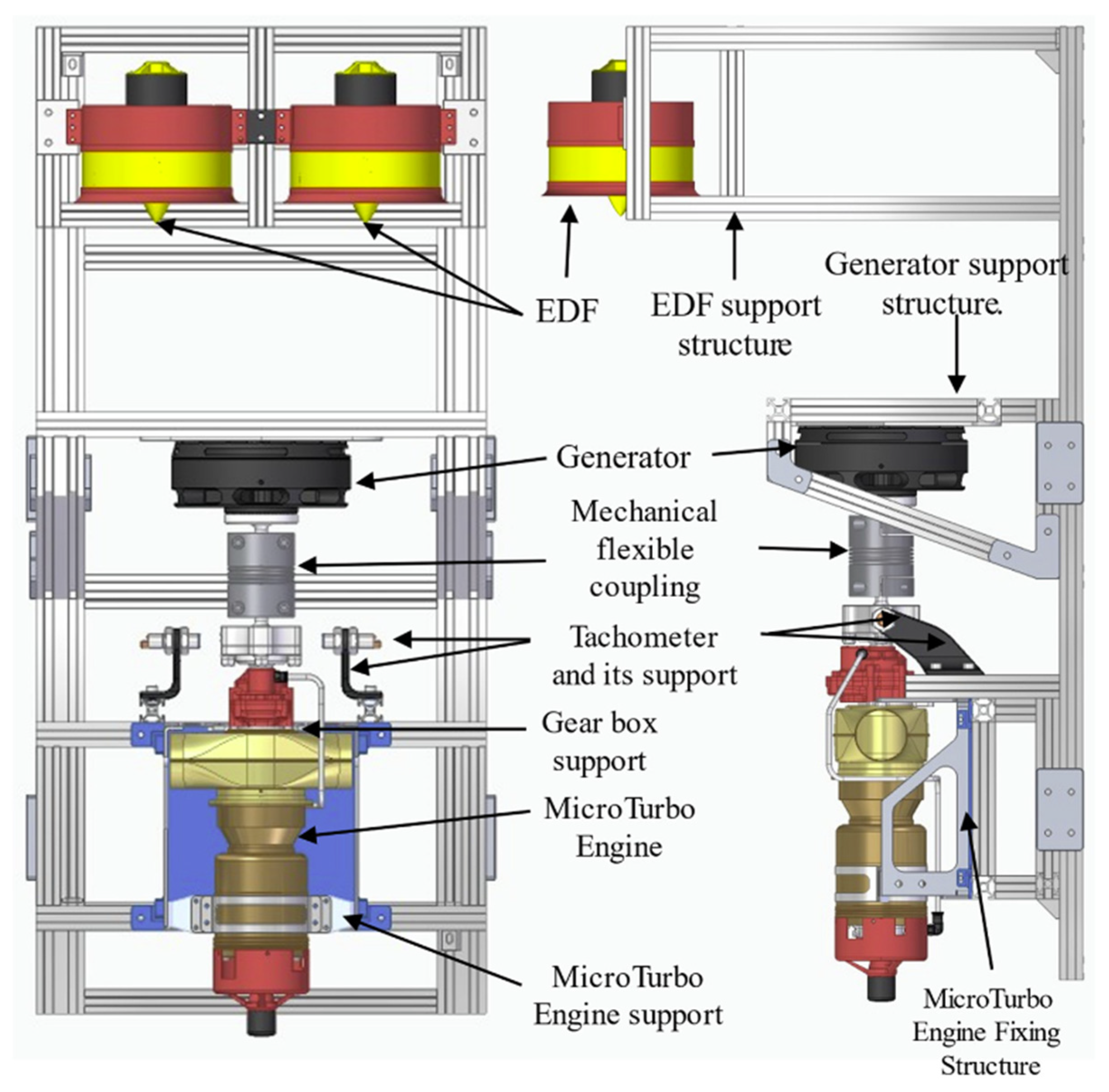
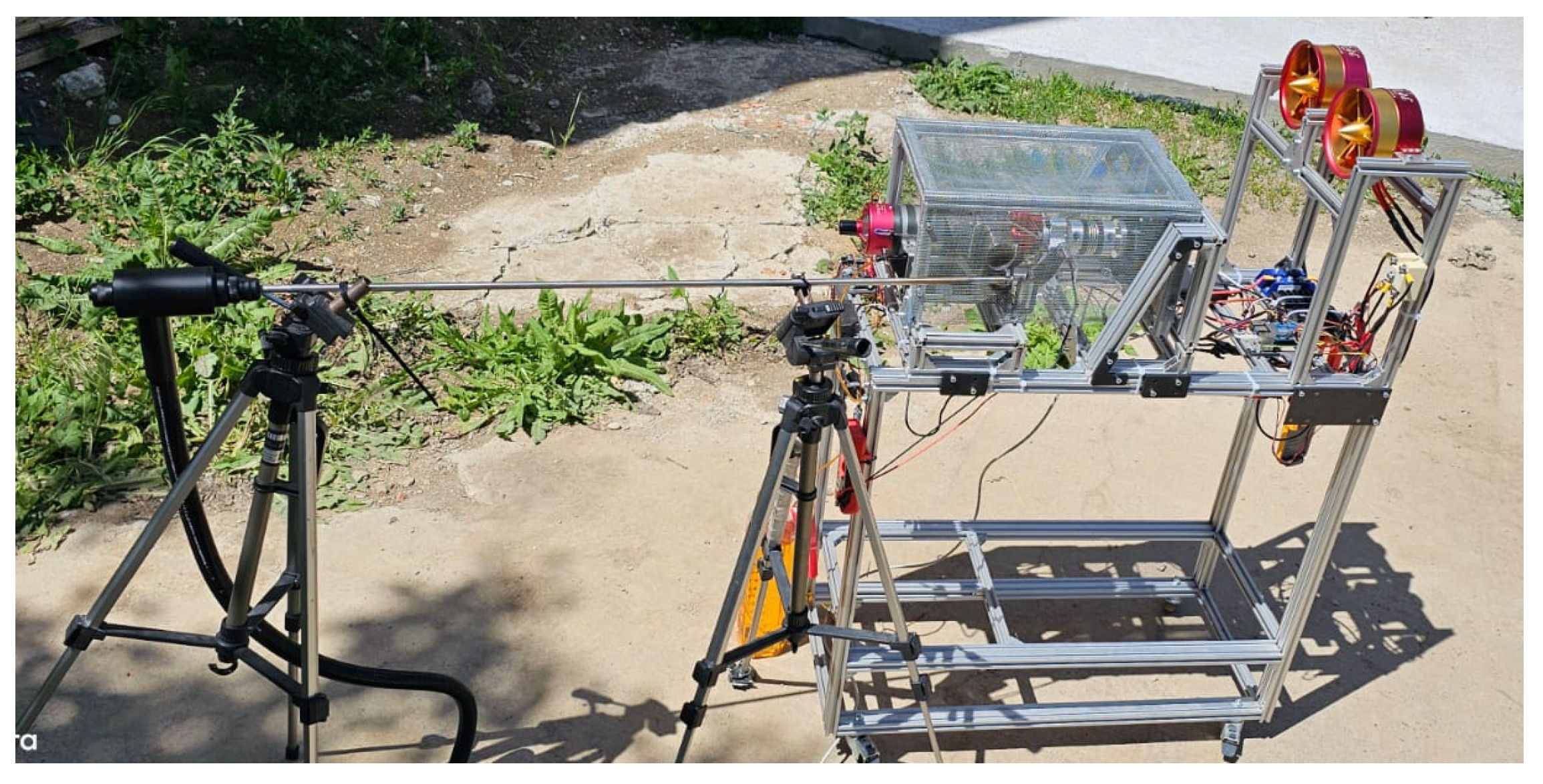
The experimental setup, illustrated in Figure 2, is centered on a KingTech micro-turboprop engine, fueled with kerosene blended with 5% AeroShell oil, an engine whose compact architecture and operating characteristics make it well suited for UAV-scale applications. This engine is mechanically coupled to a T-Motor electric generator through a flexible coupling, which mitigates misalignment stresses and reduces the transmission of vibrations. The generator’s role is to transform the shaft power of the micro-turboprop into electrical energy, which is then rectified from alternating current to direct current. A regulated 48 VDC bus forms the backbone of the electrical architecture, with a parallel battery pack included not as a primary energy source but as a stabilizing buffer, capable of absorbing transient imbalances and supplying auxiliary devices such as the electronic control unit (ECU) and fuel pumps.
The generated electrical energy is directed to two electric ducted fans (EDFs), which function as controllable load emulators. These fans replicate the aerodynamic demands typically encountered in UAV propulsion, thereby enabling a realistic assessment of how the hybrid power system would perform in actual flight scenarios. Each EDF is governed by its own electronic speed controller (ESC), which interprets control signals and regulates current draw accordingly. This dual-EDF configuration represents a significant evolution of the bench compared to earlier iterations, where a single EDF proved insufficient for accurately distributing loads and capturing the complex dynamics of UAV propulsion demand. In addition, refinements to the structural frame were necessary, as prior designs experienced destabilizing vibrations caused by the interaction of airflow with crossbeams. By reinforcing the frame and adjusting the positioning of the EDFs, the updated bench achieved far greater stability and robustness.
To enable autonomous system operation, a fuzzy logic control algorithm was implemented on a single-board computer (SBC). The controller utilized the system voltage as the primary regulation parameter, continuously adjusting the engine throttle via pulse-width modulation (PWM) control signals to maintain the DC bus voltage at 48 V. During the testing phase, however, a series of irregularities were identified in the generator’s rotational speed readings. Abnormal values were observed within the recorded data set, adversely affecting the accuracy and stability of the micro-turboprop engine’s automatic control. The initial approach to measuring rotational speed proved inadequate, as errors persisted even after optimizing the sampling interval. Although the magnitude of these errors was partially mitigated, their presence continued to induce instability during autonomous operation.
Given that the generator’s rotational speed, one of the key input parameters of the fuzzy logic controller, was not being accurately recorded, the control strategy was modified. Recognizing the direct proportionality between the generator’s rotational speed and its output voltage, the project team substituted voltage monitoring for speed measurement. Consequently, the controller’s input variable was changed from generator speed to output voltage. A significant innovation in this revised approach was the introduction of two input variables: the instantaneous output voltage and its time derivative. Incorporating the voltage derivative enabled the controller to anticipate transient responses and respond rapidly to abrupt load variations, thereby enhancing both dynamic response and steady-state stability. This modification improved the system’s adaptability to the highly variable power demands characteristic of UAV operation. Furthermore, the autonomous control system allows the entire test bench to be operated through a user-friendly interface, which facilitates seamless management of all required operating regimes, from idle to high-load conditions [32].
Experimental testing validated the capacity of the bench to deliver a stable electrical output of approximately 3 kW, with the potential to reach up to 3.5 kW under higher throttle conditions. Moreover, the bench proved capable of supporting both steady-state and transient experiments, including step-load responses, making it a versatile tool for characterizing hybrid power systems under diverse conditions.
Overall, the test bench serves as both a validation tool and a developmental platform. By integrating structural, electrical and control refinements into a coherent experimental environment, it enables reliable and repeatable assessment of hybrid powertrain performance. Its capacity to replicate UAV propulsion demands and maintain voltage stability under varying conditions highlights its significance for advancing hybrid propulsion concepts. In particular, the system demonstrates how micro-turboprop and electric generator combinations, when managed through intelligent control strategies, can substantially extend UAV range and mission versatility. This makes the bench not only a technical contribution but also a stepping stone toward the practical adoption of hybrid power solutions in next-generation UAV applications.

2.3. Experimental Strategy

When investigating the pollutant emission profile of a fuel blend, it is essential to consider two aspects: the local, instantaneous concentrations of emissions directly at the engine exhaust, and the subsequent dispersion of these pollutants in the surrounding atmosphere. To obtain a robust and representative analysis, the measurement setup was therefore composed of two complementary components. Exhaust gas measurements were conducted using the MRU GmbH Nova Plus portable combustion analyzer (Neckarsulm-Obereisesheim, Germany), provided by Mecro Systems SRL, enabling real-time quantification of exhaust gas temperature and key gaseous emissions with an accuracy level of 5%.
This instrument illustrated in Figure 3 was employed for real-time quantification of exhaust gas temperature (EGT) and gaseous emissions during engine operation. The EGT was measured directly at the exhaust stream using a high-temperature thermocouple integrated into the sampling probe, ensuring rapid thermal response and accurate tracking of transient operating conditions, particularly during regime transitions.
Gas species analysis was conducted through a combination of nondispersive infrared (NDIR) and electrochemical sensing technologies integrated within the analyzer. Carbon monoxide (CO) concentrations were determined using an NDIR sensor, which quantifies gas concentration based on selective infrared absorption at characteristic wavelengths. Nitric oxide (NO) and nitrogen dioxide (NO2) were measured via electrochemical cells, with total NOx calculated as the sum of NO and NO2 concentrations. Sulfur dioxide (SO2) was likewise quantified using a dedicated electrochemical sensor optimized for low-concentration detection.
The sampling system incorporated an internal pump to extract exhaust gases through a heated probe and particulate filter, minimizing condensation and ensuring representative sample conditioning prior to sensor exposure. Continuous data acquisition enabled synchronized recording of EGT and pollutant concentrations across different engine operating regimes, including high-power conditions and transitions toward low-power states. This configuration allowed direct correlation between thermal behavior and emission formation, supporting a detailed evaluation of combustion stability and pollutant trends under ethanol–kerosene fueling conditions.
The monitoring of pollutant dispersion was conducted using a mobile laboratory, positioned 30 m from the engine. This setup enabled the simultaneous measurement of ambient air pollutant concentrations and relevant meteorological parameters, providing insight into the spatial distribution and behavior of emissions in the surrounding atmosphere. This configuration follows the methodology previously described in [33], ensuring consistency and accuracy of the experimental results.
The mobile laboratory is equipped with reference-grade instruments (HORIBA AP360 series, provided by Horiba Romania, Kyoto, Japan) designed for the determination of major atmospheric pollutants, including CO, SOx, NOx, and O3. These analyzers exhibit high precision, with repeatability and linearity both specified at ±1% of full scale and a lower detectable limit around 0.02 ppm for CO. This indicates the instruments can produce consistent and reliable measurements across gases like CO, SO2, NOx, and O3. While precision is a key part of overall measurement uncertainty, full uncertainty also depends on calibration, environmental factors, and sampling, which are not fully specified in the datasheet.
In addition, a meteorological station was integrated into the system to continuously record wind speed and direction, air temperature, atmospheric pressure and relative humidity at a height that could reach 10 m above ground level. Air quality measurements were performed continuously throughout the experimental campaign at 10-s intervals using high-precision analyzers compliant with European reference standards. Nitrogen oxides (NO, NO2, and NOx) were quantified using a Horiba APNA-360 analyzer (Kyoto, Japan) based on the chemiluminescence principle, while sulfur dioxide concentrations were measured with a Horiba APSA-360 analyzer (Kyoto, Japan) employing ultraviolet fluorescence. Ozone levels were determined using a Horiba APOA-360 analyzer (Kyoto, Japan) operating on ultraviolet photometry, and carbon monoxide concentrations were measured with a Horiba APMA-360 analyzer (Kyoto, Japan) based on nondispersive infrared detection.
The experimental campaign focused on three ethanol–kerosene fuel blends containing 10%, 20% and 30% ethanol by volume. Each blend was tested under four distinct operating regimes representative of typical UAV propulsion conditions. Every operating regime was maintained for one minute to ensure that the recorded data reflected steady-state operation, thereby enhancing the reliability of the measurements. The tested regimes ranged from idle operation, during which both EDFs were inactive and the system operated at a supply voltage of 20 V DC, to progressively higher power states at a regulated voltage of 48 V DC. These higher regimes involved the activation of one or both EDFs to achieve an electrical power demand of approximately 1000 W, 2000 W and 2500 W, respectively, thereby simulating increasing propulsion loads encountered during UAV operation.
The parameters recorded during the tests were grouped into three main categories. The first category included operational data acquired by the test bench sensory system, such as the throttle position of the micro-turboprop engine and the electrical characteristics of the system, including voltage, current, and power output, all recorded at a sampling rate of one second. The second category comprised spatially resolved measurements of atmospheric pollutants obtained using the mobile environmental monitoring system. The third category focused on exhaust-related parameters, including exhaust gas temperature and the concentration of pollutant species in the exhaust stream, measured using a dedicated exhaust probe. The gaseous pollutants measurements made both at the exhaust of the engine and in a certain distance allows the drafting of wind rose and the dispersion charts of the pollutants. Thus, by analyzing the meteorological parameters and the evolution of gaseous pollutants concentrations, the evaluation of those concentrations beyond the position of the mobile lab is made possible.
Figure 4 shows the placement of the engine, mobile lab and residential area.
As can be seen, the experimental setup was made so that the engine (the source of pollutants) was at least 100 m from the residential area, but the second set of measurements was performed 30 m from the position of the mobile lab.
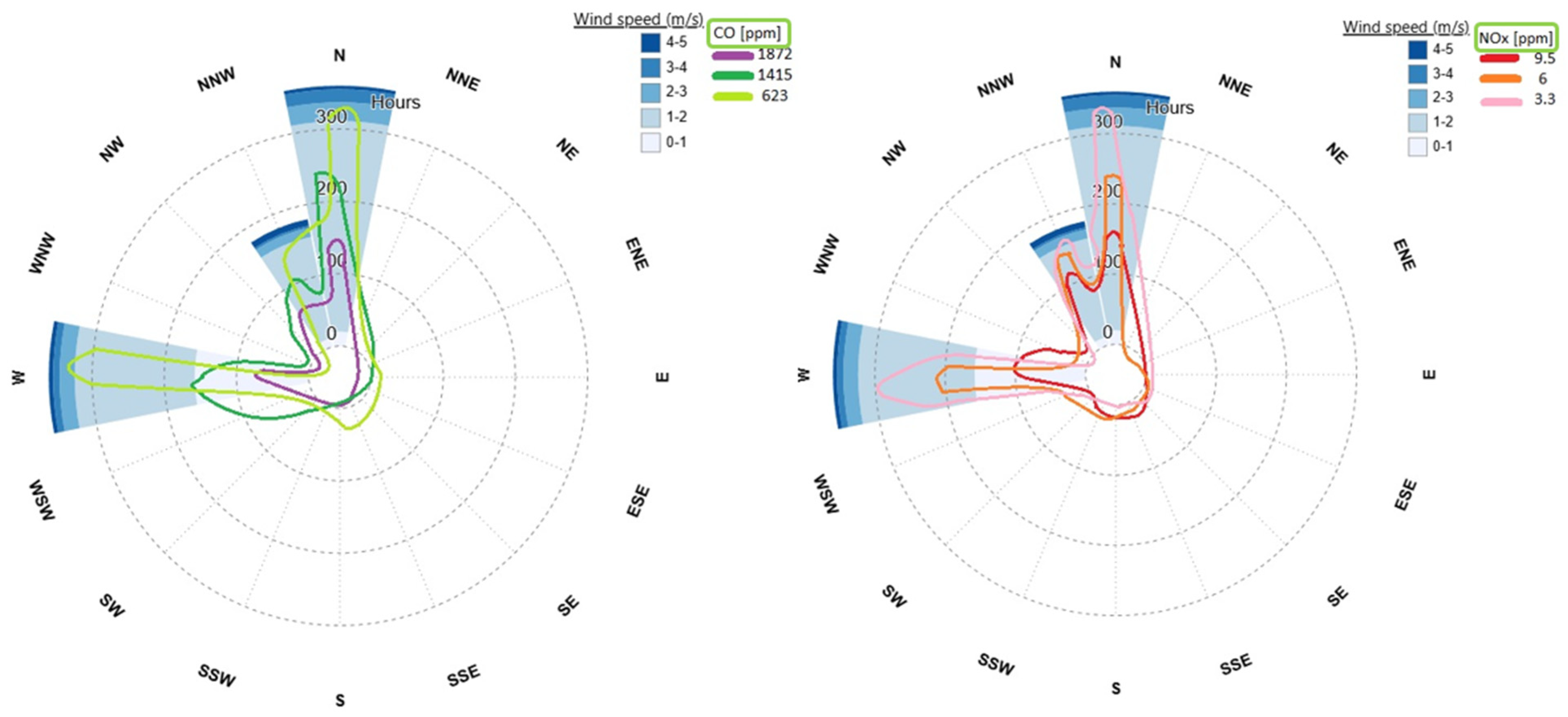
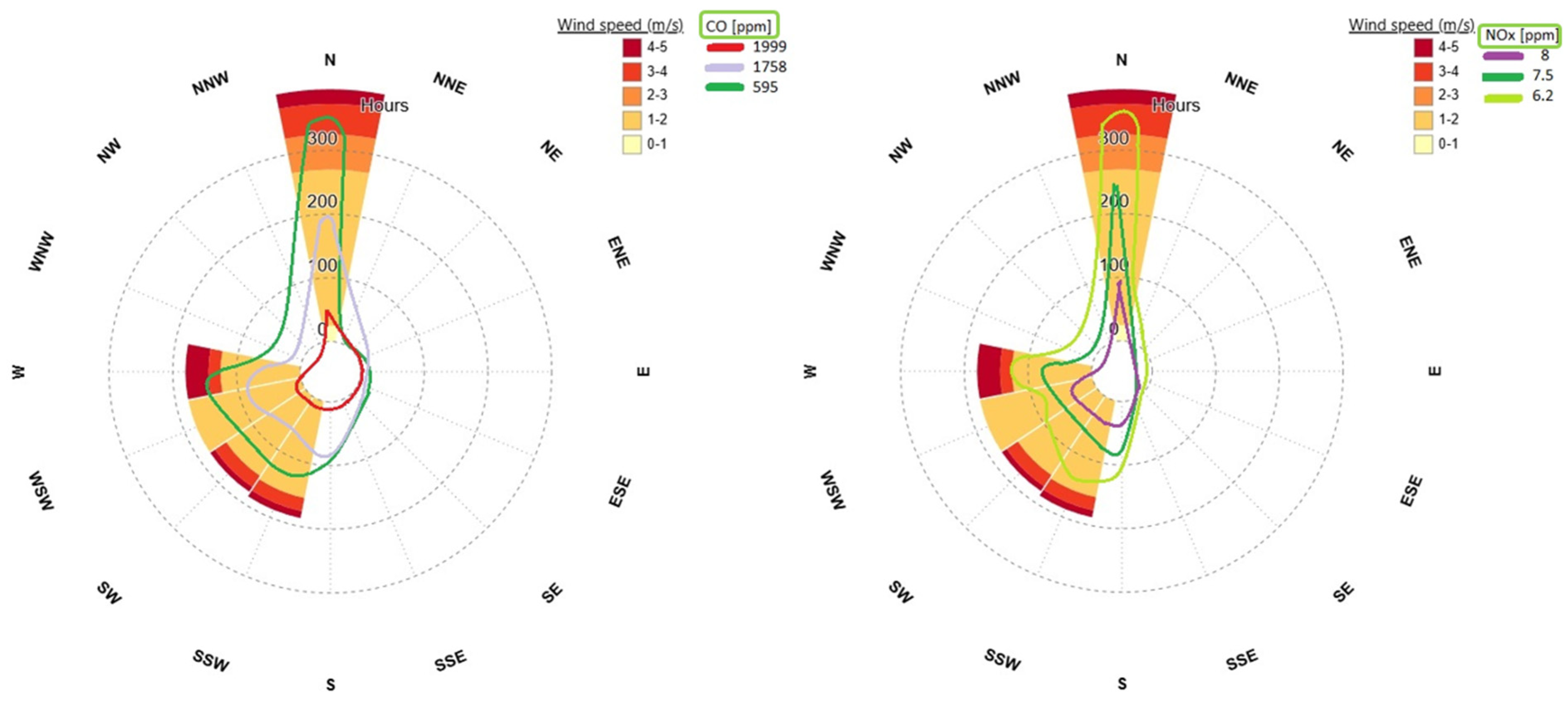
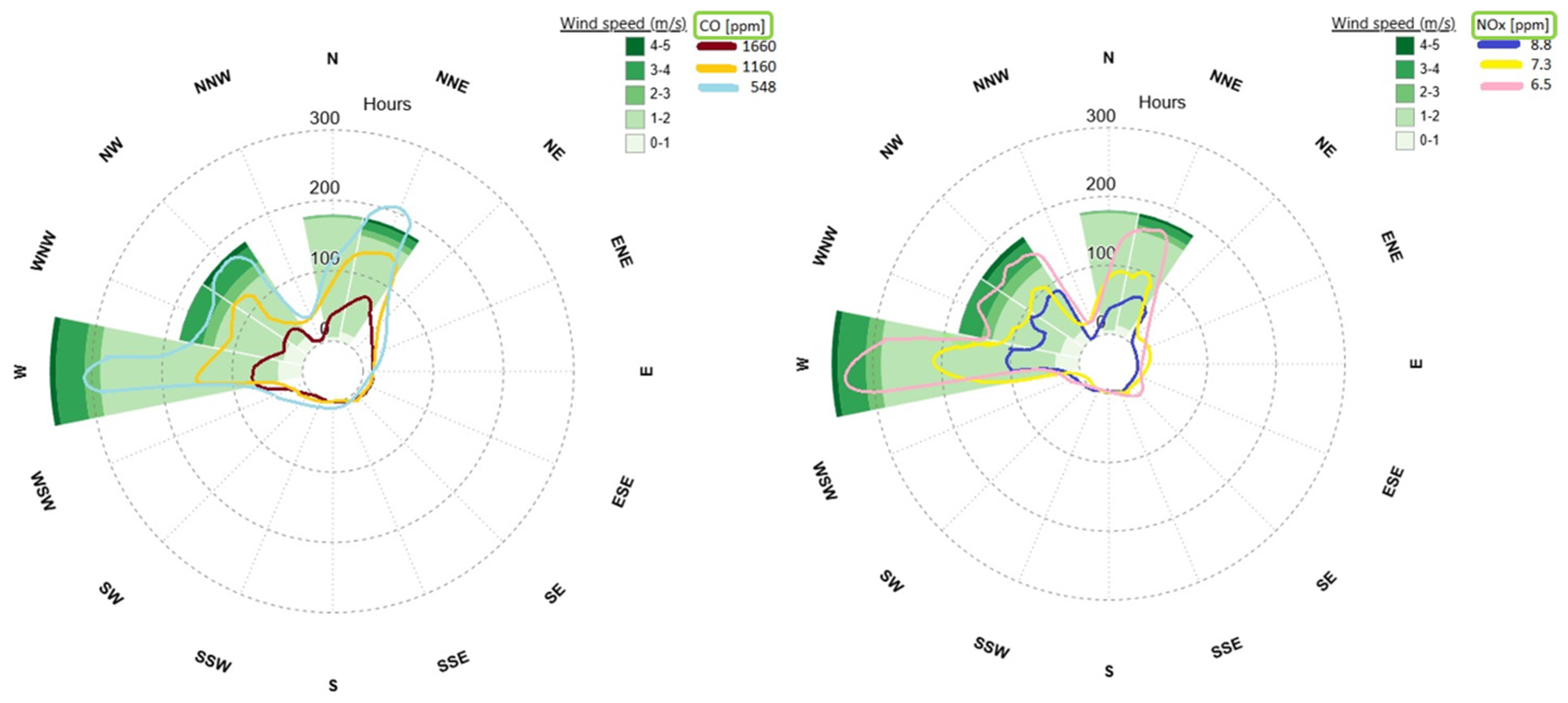
Figure 5, Figure 6 and Figure 7 show wind roses for the 3 experiments (10, 20 and 30% ethanol) and also highlight the evolution of the main pollutants (CO and NOx) in the direction of the wind. The evolution of SO2 was excluded from this analysis because the recorded concentrations were negligible, thereby limiting their relevance to the study.
As can be observed from Figure 5, Figure 6 and Figure 7, wind speed and direction greatly influence the distribution of gaseous pollution. The engine (the pollutant source) is situated in the center of the plot and wind speed and direction within the timeframe of experimental measurements are represented in the wind rose. As shown in Figure 6, Figure 7 and Figure 8, wind speed and wind direction exert a significant influence on the spatial distribution of gaseous pollutants. In each polar diagram, the microturbine engine, representing the emission source, is positioned at the center of the plot, while the wind rose illustrates the frequency and distribution of wind directions recorded during the measurement period. The pollutant concentration overlays integrated into these plots allow a direct correlation between meteorological conditions and pollutant dispersion patterns.
The figures clearly indicate that the pollutant plume is transported predominantly in the direction of the prevailing wind, confirming that atmospheric advection represents the primary mechanism controlling pollutant transport from the source. As the wind carries the emitted gases away from the engine, the dispersion domain becomes elongated along the dominant wind direction, reflecting the main pollutant transport pathway. This behavior is characteristic of buoyant plumes generated by combustion systems, where the combined effects of exhaust gas momentum and atmospheric wind determine plume trajectory and dilution.
An important observation is that pollutant concentration decreases with increasing wind speed. Higher wind velocities enhance turbulent mixing and atmospheric dilution processes, resulting in a more rapid reduction in pollutant concentration as the dispersion domain expands over a larger area. Conversely, low wind speeds are associated with higher local pollutant concentrations, as the reduced airflow limits dilution and allows pollutants to accumulate in the vicinity of the emission source. This behavior confirms that atmospheric dilution is inversely proportional to pollutant concentration for a constant emission rate.
These dispersion maps highlight the combined influence of emission intensity and atmospheric conditions on pollutant transport. Engine operating parameters and fuel composition determine the initial pollutant concentration at the source, while the local wind regime controls the direction, dispersion rate, and spatial extent of the pollutant plume. Therefore, the presented figures do not merely illustrate the geometric dispersion of emissions but also demonstrate the strong dependence of ground-level pollutant concentration on atmospheric dynamics, particularly wind speed and direction.
From an environmental impact perspective, this result is significant because it shows that pollutant concentration at a given location is not determined solely by emission rate but also by meteorological conditions. Under low wind conditions, even relatively small emission rates can result in locally elevated pollutant concentrations, whereas under high wind conditions, the same emission rate can lead to significantly lower ground-level concentrations due to enhanced dilution. This finding is particularly relevant for UAV or small-scale turbine operation in confined or urban environments, where local meteorological conditions can strongly influence pollutant exposure levels.
Furthermore, differences between fuel blends can also be observed in the dispersion maps, as blends producing higher CO emissions at the source also generate higher concentration zones in the downwind direction. However, the spatial distribution pattern remains primarily governed by wind direction, indicating that atmospheric transport dominates over emission anisotropy in determining plume geometry, while emission intensity controls concentration magnitude.
Overall, the dispersion analysis demonstrates that pollutant transport from the microturbine exhaust is governed by two main mechanisms: emission intensity at the source, which depends on fuel composition and engine operating regime, and atmospheric dispersion, which depends primarily on wind speed and direction. The combined effect of these parameters determines the final spatial distribution of pollutants and their potential environmental impact.

3. Results

Experimental Testing Campaign

The following section presents and analyzes the experimental results obtained during the testing campaign of ethanol–kerosene fuel blends on the micro-turboprop engine test platform. The data sets collected encompass both the engine’s operational parameters and the corresponding emission characteristics, providing a comprehensive assessment of the blends’ performance under various operating regimes. To improve clarity and avoid redundancy, the emission results are presented in consolidated figures, where multiple pollutant species are plotted together as a function of operating regime, allowing direct comparison between fuels and pollutants. The first component of the analysis involves a systematic assessment of the effect of fuel composition on operational parameters, such as the EGT, the electrical output and the pollutant concentration levels. The results are discussed in relation to the engine’s overall efficiency and environmental impact, offering insight into the feasibility of using ethanol–kerosene mixtures as alternative fuels for small-scale aviation applications.
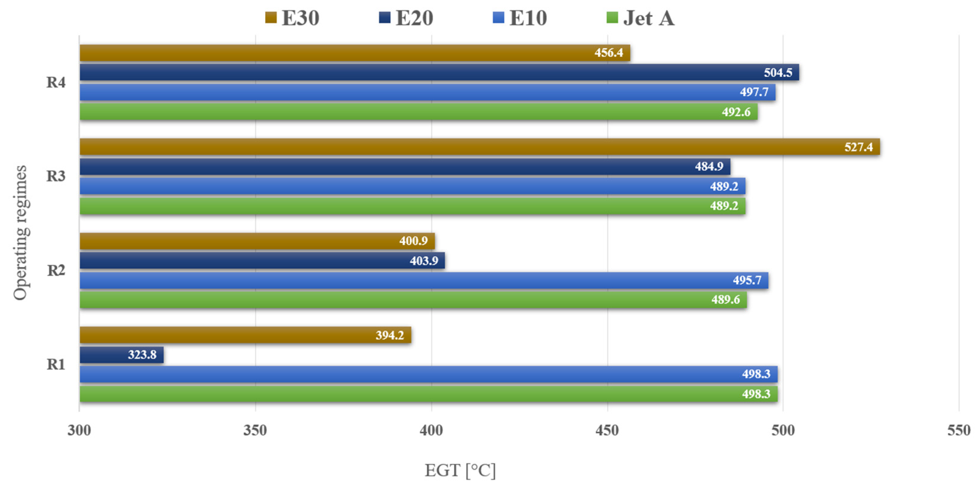
Figure 8 compares the Exhaust Gas Temperature (EGT) profiles of three ethanol–kerosene blends against pure kerosene. The E10 blend (10% ethanol, 90% kerosene) exhibits behaviour most similar to pure kerosene. In the higher operating regimes, its EGT exceeds that of the baseline fuel by only a few degrees. Furthermore, the EGT values for E10 show minimal variation across the four operating regimes, a characteristic also observed with pure kerosene. This similarity is not evident in the other two blends. The E20 blend (20% ethanol, 80% kerosene) demonstrates a gradual increase in EGT, while the E30 blend (30% ethanol, 70% kerosene) exhibits a more pronounced and erratic behavior. The E30 blend recorded the highest EGT of all fuels tested, reaching a peak value of 527 °C.
From a sustainability standpoint, the foremost priority lies in mitigating the emission of toxic chemical species generated during combustion, a concern that surpasses the significance of the EGT itself. Nevertheless, EGT retains a tangible and meaningful influence on pollutant formation, as it reflects the combustion temperature that governs the generation of key contaminants such as NOx, CO and unburned hydrocarbons [34,35]. Accordingly, monitoring EGT is valuable not solely as a performance indicator but as an informative parameter for interpreting and optimizing the engine’s emissions behavior, particularly when evaluating the effects of alternative fuels, such as ethanol–kerosene blends, on temperature-dependent reaction pathways [36].
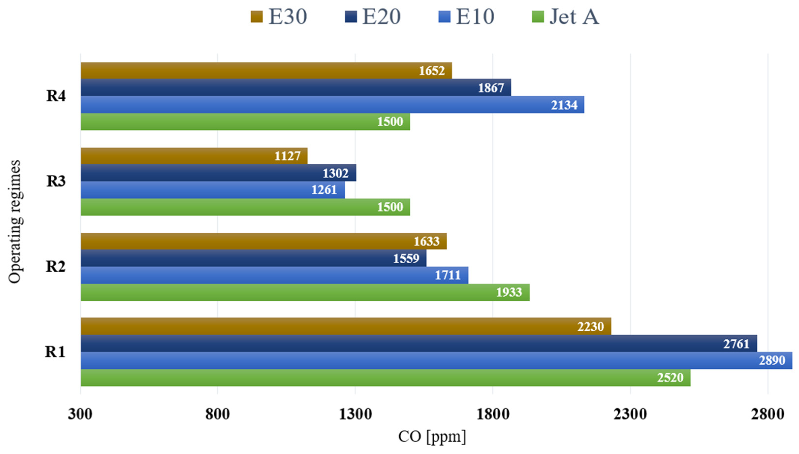
CO represents one of the most prevalent pollutant species unavoidably generated during the combustion of hydrocarbon fuels, and is shown in Figure 9, which presents the variation in CO emissions for all tested fuels across the four operating regimes. As CO emissions are closely associated with incomplete combustion, their magnitude serves as a reliable indicator of combustion efficiency. Consequently, the highest CO concentrations are observed under idle conditions, which are well known to correspond to one of the least efficient operating regimes. This behavior persists for both ethanol–kerosene blends and neat kerosene. Notably, the E10 and E20 blends exhibit comparable trends, characterized by elevated CO levels during the idle and fourth regimes, reaching a maximum of almost 2900 ppm (parts per million), and marginally reduced concentrations relative to kerosene under the intermediate regimes (2 and 3). The E30 blend, however, exhibits the lowest CO emissions, performing even better than pure kerosene in the first three operating regimes. In the final regime, its CO emissions exceed those of kerosene by only approximately 10%.
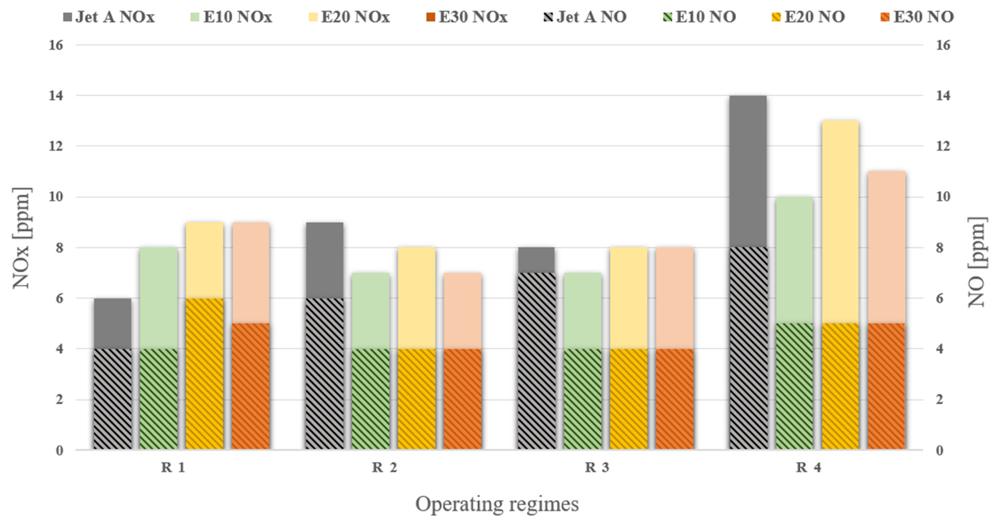
Nitrogen oxide emissions, including NO and total NOx, are presented together in Figure 10 to allow direct comparison between the two species and across operating regimes. The influence on nitrogen oxides is more complex, as NOx formation depends primarily on flame temperature and oxygen availability, meaning that oxygenated fuels may either increase or decrease NOx depending on the resulting combustion temperature field.
It is evident that the ethanol–kerosene blends produce substantially lower amounts of NO compounds compared to pure kerosene, particularly at higher operating regimes. During the idle regime, however, the E20 and E30 blends recorded slightly higher NO levels than both kerosene and the E10 blend. The comparison between NO and NOx indicates that NOx concentrations are consistently higher than NO alone, particularly in the fourth operating regime, indicating the presence of NO2 formation at higher combustion temperatures.
The data presented in Figure 10 clearly indicate that, for ethanol–kerosene fuel blends, the total concentration of NOx markedly exceeds that of NO alone, fact which was to be expected. This effect is particularly pronounced in the fourth operating regime, where the overall NOx levels approach or surpass twice the NO fraction in the exhaust gases. The highest NOx concentration is observed for neat kerosene, reaching approximately 14 ppm, followed by the E20 blend, which likewise displays more than double the NO content under comparable conditions. It is further observed that the NOx concentration reaches its maximum in the fourth operating regime for all tested fuels, including pure kerosene, contrasting with the CO emissions, which peak during the idle regime. Among the ethanol–kerosene blends, the E10 mixture exhibits the lowest overall NOx emissions, performing slightly better than kerosene when evaluated from a global perspective of the experiment.
A possible cause of these variations in NOx emissions is the cetane number of the fuel blends. The addition of ethanol to kerosene reduces the overall cetane number of the blend due to the low autoignition quality of ethanol. A lower cetane number leads to a longer ignition delay period, which increases the premixed combustion phase and can result in higher peak combustion temperatures [37]. Since thermal NOx formation is strongly temperature-dependent and follows an exponential relationship with flame temperature, an increase in peak combustion temperature can promote higher NOx formation despite the lower carbon content of the fuel [38]. On the other hand, longer ignition delay may also improve fuel–air mixing, which can reduce carbon monoxide emissions by promoting more complete combustion. Therefore, the cetane number influences a trade-off between CO and NOx emissions through its effect on ignition delay, combustion temperature, and mixture formation [39].
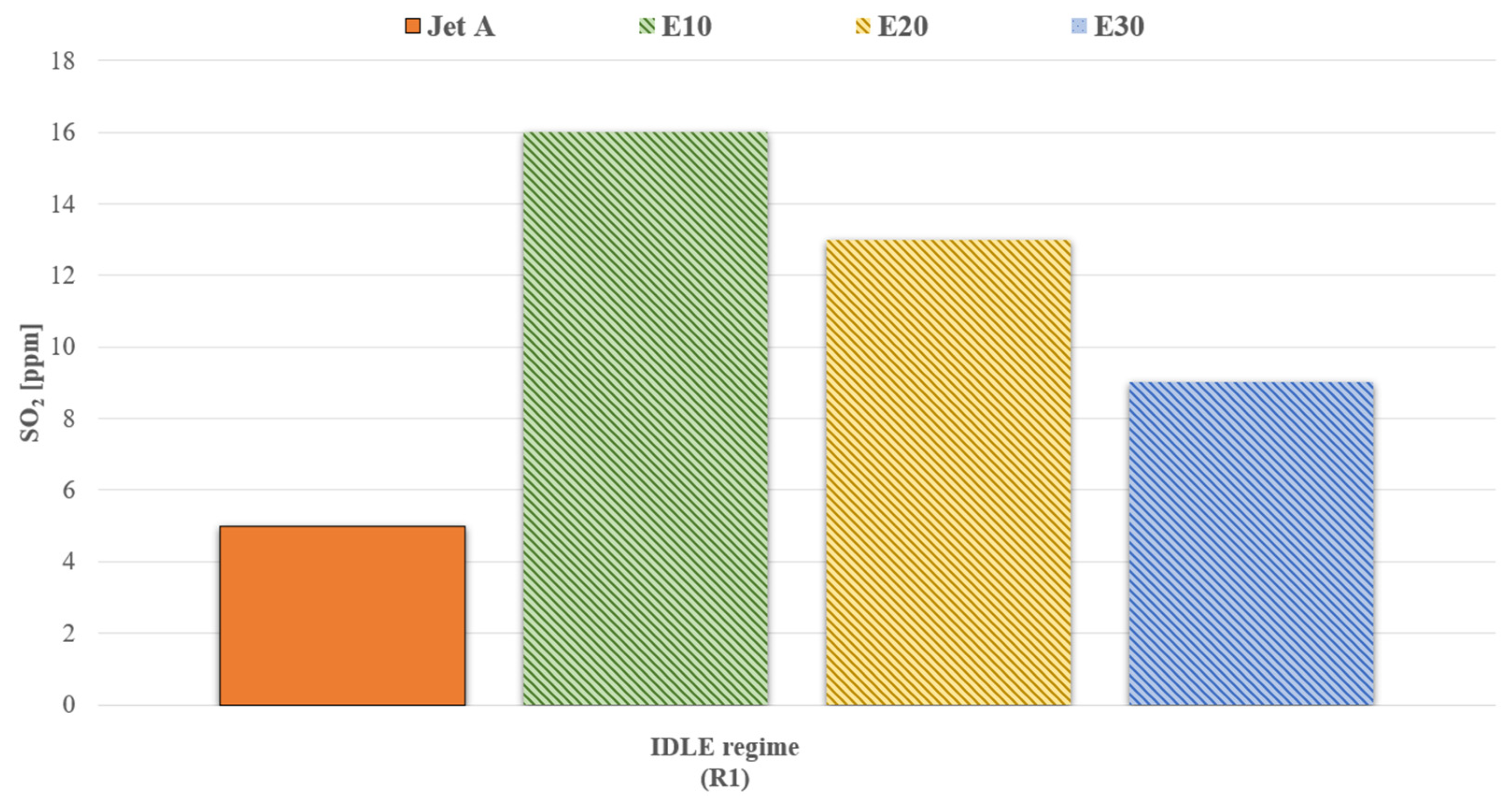
Another pollutant species examined during this experimental campaign, and one of particular relevance from a sustainability standpoint, is sulfur dioxide (SO2). Unlike the other chemical pollutants analyzed thus far, SO2 is not expected to form based on the theoretical combustion reactions of any of the tested fuel blends. Even the lubricating oil used to ensure the micro-turboprop engine’s longevity is sulfur-free. Nevertheless, the kerosene sample was found to contain traces of sulfur oxides, a phenomenon commonly encountered in the aviation sector due to fuel contamination that can occur during refining [40,41], storage or handling processes. Nevertheless, due to the reduced quantity of sulfur atoms, the SO2 molecules were only registered during the idle regime, with its variation presented in Figure 11.
A notable finding is that the measured SO2 concentrations are of a similar order of magnitude to those observed for the NOx compounds. Among the tested fuels, pure kerosene exhibits the lowest SO2 emissions, while the E10 blend produces the highest concentrations, reaching up to 16 ppm. Within the ethanol–kerosene mixtures, the E30 blend demonstrates the most favorable performance, yielding the lowest SO2 emissions among the blended fuels, although these values remain almost twice as high as those measured for pure kerosene.
The second part of the analysis focuses on the influence of ethanol–kerosene fuel blends on the performance characteristics of the micro-turboprop engine, with particular emphasis on electrical power output, the primary parameter of the test bench and the key performance requirement for the unmanned aerial vehicle (UAV) to be powered by it. The electrical power was determined from the measured voltage and current intensity values, which were recorded using a Hall-effect current sensor (Mateksys, Shenzhen, China). In addition to these parameters, other significant variables were also monitored, including the rotational speed of the electric generator and the throttle setting of the micro-turboprop engine. It is important to note that, within the context of this study, the term throttle differs from its conventional use in gasoline engines. Unlike gasoline engines, where a throttle valve regulates air intake, the operation of the micro-turboprop engine is controlled by adjusting the quantity of fuel supplied. Consequently, throughout this analysis, the term throttle specifically refers to the power output level corresponding to the rate of fuel delivery to the combustion chamber of the micro-turboprop engine.
The efficiency of the three fuel blends relative to kerosene is evaluated by comparing their throttle requirements across different engine operating regimes. This analysis determines whether a blend consumes more or less fuel to deliver a specific level of electrical power. To properly evaluate each blend’s performance, we used the experimental data recorded by the test bench sensors to establish a mathematical relationship between the throttle position and the electrical power output. This was accomplished through polynomial regression, a method for fitting a smooth curve to discrete experimental measurements.
The method uses a discrete set of experimental data points ( x i , y i ) , where x i represents the throttle level and y i the corresponding electrical power output. From these points, it derives a continuous polynomial function f ( x ) of degree n that models their relationship:
f x = i = 0 n a n i x i
The coefficients a i are determined by minimizing the total squared deviation between the experimental data and the polynomial model, expressed as
S = i = 1 m ( y i f ( x i ) ) 2
where y i represents the real actual value of the electrical power, which was experimentally obtained and f ( x i ) represents the approximated value, which derived from the polynomial function.
This minimization corresponds to a least-squares optimization, ensuring that the fitted curve best represents the experimental trend in a statistical sense. The optimal polynomial degree n can either be chosen based on theoretical considerations or determined empirically by evaluating the coefficient of determination, R 2 , for successive degrees:
R 2 = 1 i = 1 m ( y i f ( x i ) ) 2 i = 1 m ( y i y - ) 2
where y - denotes the mean of the measured values. The selection of the optimal polynomial degree is based on the R 2 metric. The degree that yields the highest R2 is considered to provide the most appropriate balance between descriptive accuracy and model simplicity, thereby avoiding both underfitting and excessive complexity. Furthermore, to maintain physical consistency in cases where the measured quantity cannot assume negative values, the fitted function is shifted vertically such that f ( x ) > 0 for all x within the experimental domain. This adjustment ensures that the regression respects the constraints inherent to the physical system.
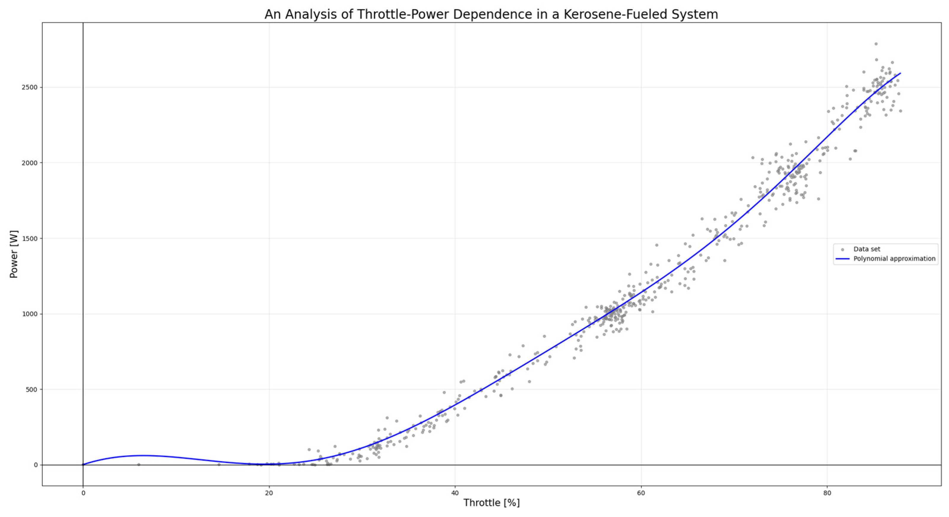
Once determined, the resulting polynomial functions serve as continuous analytical representations of the experimental data. Figure 12 illustrates the experimental data points together with the polynomial approximation of the dataset obtained from the test conducted using kerosene. The higher concentration of data points at certain power levels arises from the need to ensure adequate sensor precision for the reliable acquisition of pollutant measurements.
The polynomial function that characterizes the relationship between the electrical power consumption and the throttle level when using kerosene as fuel is defined as follows:
f n x = a 0 x 7 + a 1 x 6 + a 2 x 5 + a 3 x 4 + a 4 x 3 + a 5 x 2 + a 6 x 1 + a 7
where the coefficients have the following values:
a 0 = 6.03852 ×   10 10 a 1 = 3.59537   ×   10 8         a 2 = 2.00734   ×   10 5         a 3 = 3.29819   ×   10 3 a 4 = 0.19901                                   a 5 = 4.755195                       a 6 = 41.88344                               a 7 = 65.186075                
Following an identical mathematical formulation, the polynomial coefficients obtained from fitting the experimental data for each ethanol–kerosene blend are reported in Table 3. The optimal polynomial approximation used to interpret the data obtained from testing the ethanol–kerosene blend with a 10–90 mixing ratio has a polynomial degree of six; consequently, the final two coefficients are zero. A similar situation applies to the polynomial approximation for the 20% ethanol blend, which has a polynomial degree of seven.
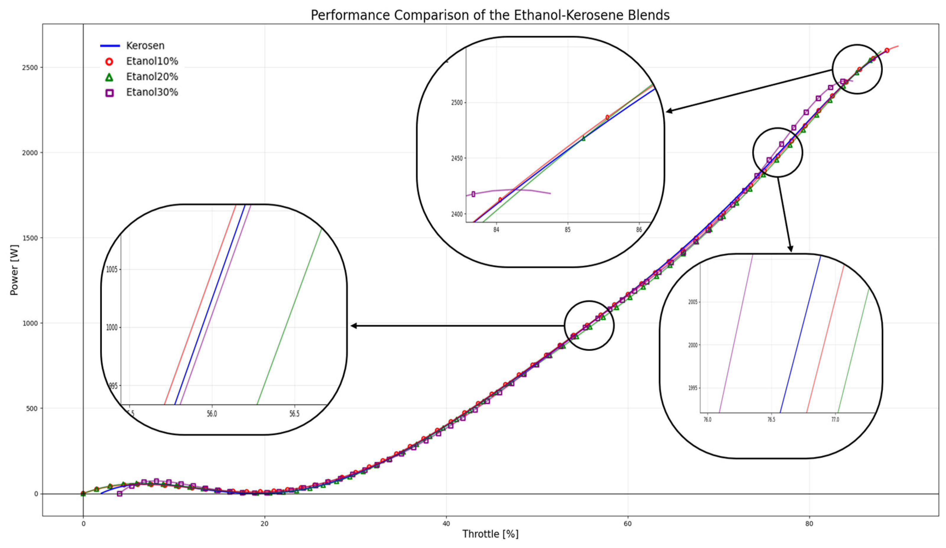
As a result, the polynomial approximation functions providing the best fit for the three ethanol–kerosene blends are shown in Figure 13.
The overall behavior of the alcohol–kerosene blends is largely comparable to that of neat kerosene, with only minor differences observed in the throttle settings required to achieve the prescribed power levels. At the 1000 W operating regime, the E10 and E30 blends exhibit performance closely matching that of kerosene, requiring nearly identical throttle positions. In contrast, the E20 blend requires a slightly higher throttle level, exceeding 56%, to attain the same power output. A similar trend is observed at the 2000 W regime, where E20 again demands the highest throttle input, reaching approximately 77%, while the remaining blends remain closer to the kerosene baseline. At the highest tested power level, the E20 blend demonstrates improved performance, achieving marginally higher output than kerosene. Conversely, although the E30 blend is capable of reaching the target power, it fails to sustain this level over the entire test duration. This limitation is not related to the polynomial approximation method used for data processing, but rather to the physical and thermodynamic characteristics of the fuel blend. The higher ethanol content reduces the lower heating value of the fuel and increases the latent heat of vaporization, which leads to a reduction in combustion temperature and, consequently, in turbine inlet temperature. Since turbine power is directly dependent on turbine inlet temperature, the available mechanical power to drive the compressor and generator decreases, making it difficult for the engine to maintain the required rotational speed and electrical output under high-load conditions. As a result, the engine operates closer to its stability limit when fueled with the E30 blend, which explains the observed inability to sustain the target power level for extended periods.
During the testing campaign, once the engine reached an electrical power output of 2500 W and the required emission data had been collected, the shutdown sequence of the micro-turboprop engine was initiated. This procedure involved a controlled but rapid reduction in power from 2500 W to the idle regime, followed by a short period of stabilized idle operation prior to complete engine shutdown. Such shutdown procedures are routinely performed during operation with conventional kerosene fuel and typically do not result in combustion instability.
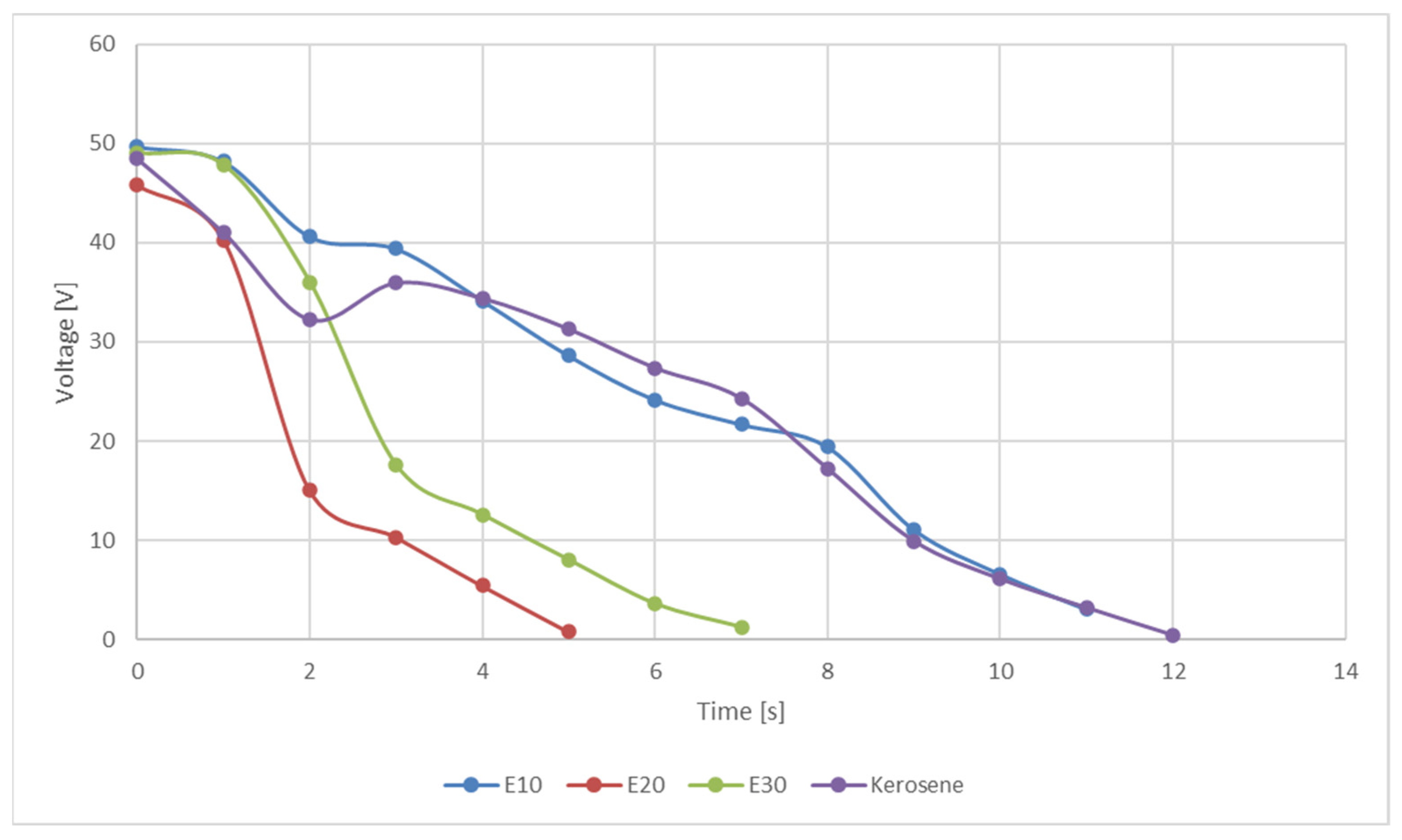
However, as the ethanol concentration increased, the transition from high-load to idle operation became progressively less stable, as reflected by the steeper voltage decay observed for the E20 and E30 blends compared to neat kerosene and the E10 blend. Since electrical power output is directly related to turbine shaft power, the observed voltage drop indicates a rapid reduction in turbine power during the load reduction phase. This behavior suggests that the combustion process was unable to sustain sufficient turbine inlet temperature during the transient regime.
From a combustion perspective, this behavior can be explained by the combined effects of rapid fuel flow reduction and delayed compressor airflow response. During throttle reduction, the fuel mass flow decreases almost instantaneously, while the air mass flow remains temporarily high due to the rotational inertia of the compressor. This results in a transient increase in the air–fuel ratio and a corresponding decrease in equivalence ratio, potentially pushing the mixture toward ultra-lean conditions close to the lean blowout limit.
This effect is further amplified for ethanol–kerosene blends due to the lower heating value of ethanol and its significantly higher latent heat of vaporization compared to kerosene. The increased evaporative cooling reduces the local flame temperature and slows chemical reaction rates, while the lower energy density reduces the heat release rate required to sustain stable combustion at idle conditions. As a result, the flame becomes unstable or extinguishes before a stable idle regime can be established, which explains why stabilized idle operation was not observed for the E20 and E30 blends. Figure 14 illustrates the final stage of the experimental campaign and shows the significantly steeper voltage decline observed for the E20 and E30 blends relative to neat kerosene and the E10 blend.
If stable idle operation had been maintained, even for a short duration, a change in the slope of the voltage trendline would be expected, reflecting a transient stabilization of the electrical output. This behavior is evident only for the kerosene case, reinforcing the interpretation that higher ethanol fractions adversely affect idle stability in the tested micro-turboprop power generation configuration.

4. Discussion

Testing revealed that all three ethanol-containing fuel blends performed largely on par with conventional kerosene. Nevertheless, variations in emissions and engine responses indicate that the concentration of ethanol plays a role in modifying both combustion efficiency and environmental impact.
From an emissions standpoint, carbon monoxide is a major concern, as it is both one of the most common and one of the most quantitatively abundant products of the combustion process. Measurements conducted on the three ethanol-blended fuels indicate that the E30 blend exhibited the lowest CO emissions overall, outperforming even conventional kerosene, which showed superior performance only at the highest operational regime. The E20 blend ranked second, displaying slightly higher CO emissions than E30 in the third operational regime, and consistently higher emissions than E30 under the highest operational conditions. These results suggest that increasing ethanol concentration can effectively reduce CO emissions across most operating regimes, highlighting the potential environmental benefit of higher ethanol blends.
Across all tested fuel blends, the measured SO2 concentrations were markedly lower than those of CO, differing by approximately two orders of magnitude. The results further indicated that SO2 emissions were detected only under the idle operating regime. Although sulfur is inherently present in kerosene due to its origin from crude oil, the addition of ethanol, which effectively reduces the kerosene fraction in the fuel blend, was observed to increase SO2 emissions. This effect may be attributed to the oxygenated nature of ethanol, which can alter combustion chemistry and promote more complete oxidation of sulfur-containing species to SO2. Among the three ethanol–kerosene blends, the E30 blend exhibited the lowest SO2 emissions. This can be explained by the combined effect of a reduced kerosene fraction, resulting in fewer sulfur atoms, and an increased ethanol fraction, providing additional oxygen that influences sulfur oxidation. Nevertheless, even the E30 blend produced slightly higher SO2 emissions than pure kerosene under the tested conditions.
Nitrogen oxides generated during the combustion process were found to be of the same order of magnitude as sulfur oxides. Among the tested fuels, the E10 blend exhibited the lowest NOx emissions across most operating regimes, outperforming kerosene except under idle conditions, where kerosene produced the least NOx. Notably, unlike CO, whose formation tends to decrease with increasing exhaust gas temperature and power output, NOx emissions were observed to increase with higher power levels. This behavior can be attributed to the temperature-dependent nature of NOx formation, as higher combustion temperatures promote the oxidation of atmospheric nitrogen into nitrogen oxides.
To interpret the experimentally observed abrupt shutdown events during rapid transitions from maximum to idle operation, the transient evolution of mixture strength was examined through a first-order air–fuel ratio and equivalence ratio analysis. The objective of this analysis was to determine whether, during throttle-down, the combustor momentarily operates below its lean stability threshold due to the different dynamic responses of fuel flow control and compressor airflow.
The stoichiometric air–fuel ratio of the blended fuels was determined using the reciprocal mixing relation
1 A F R s t , b l e n d = x A F R s t , E t O H + 1 x A F R s t , J e t A 1
where A F R s t , b l e n d is the stoichiometric air–fuel ratio of the ethanol–kerosene mixture (mass of air required per unit mass of blended fuel for complete combustion), A F R s t , E t O H is the stoichiometric air–fuel ratio of pure ethanol, A F R s t , J e t A 1 is the stoichiometric air–fuel ratio of neat Jet A1, x is the ethanol mass fraction in the blend, and 1 x represents the kerosene mass fraction. This relation expresses that the effective stoichiometric requirement of the blend is governed by the weighted contribution of each component based on mass fraction. Because ethanol contains chemically bound oxygen, A F R s t , E t O H is lower than A F R s t , J e t A 1 , and therefore increasing x reduces A F R s t , b l e n d .
The instantaneous mixture strength is expressed using the equivalence ratio,
ϕ = A F R s t A F R a c t u a l ,
where A F R s t is the stoichiometric air–fuel ratio of the fuel or blend considered, and A F R a c t u a l is the actual operating air–fuel ratio. When ϕ = 1 , the mixture is stoichiometric; when ϕ < 1 , the mixture is lean (excess air); and when ϕ > 1 , the mixture is rich (excess fuel).
The actual air–fuel ratio is defined as follows:
A F R a c t u a l = m ˙ a m ˙ f ,
where m ˙ a is the air mass flow rate entering the combustor (mass of air per unit time) and m ˙ f is the fuel mass flow rate injected into the combustor (mass of fuel per unit time). This expression represents the instantaneous mass of air supplied per unit mass of fuel and reflects the balance between compressor airflow and fuel metering.
In this regime, stable flame anchoring is maintained by swirl-induced recirculation of hot combustion products. During a rapid throttle-down command, however, the fuel mass flow rate m ˙ f decreases almost immediately due to the fast dynamic response of the fuel control system. In contrast, the air mass flow rate m ˙ a does not decrease at the same rate because it depends on compressor rotational speed, which decays according to the mechanical inertia of the rotating turbomachinery assembly.
Immediately following throttle reduction, the air mass flow rate can therefore be approximated as remaining near its maximum-load value while the fuel mass flow rate approaches its idle value. Under these transient conditions, the equivalence ratio becomes
ϕ t r a n s i e n t = A F R s t   m ˙ f , i d l e m ˙ a , m a x ,
where ϕ t r a n s i e n t is the instantaneous equivalence ratio during the initial phase of the transition, m ˙ f , i d l e is the fuel mass flow rate corresponding to idle operation, and m ˙ a , m a x is the air mass flow rate corresponding to the preceding maximum-power condition. This expression captures the dynamic imbalance created by rapid fuel reduction combined with temporarily sustained airflow.
Because m ˙ f , i d l e is significantly smaller than the maximum fuel flow while m ˙ a , m a x remains high, the ratio m ˙ f , i d l e / m ˙ a , m a x becomes very small, driving ϕ t r a n s i e n t to values well below its steady idle level. For higher ethanol blends, the reduced A F R s t further lowers ϕ t r a n s i e n t , intensifying the ultra-lean excursion.
Sustained combustion requires that the time required for heat-releasing reactions to proceed ( τ c h e m ) remains shorter than the average time reactants remain in the high-temperature region ( τ f l o w ). This inequality represents the stability condition for continuous combustion. During the transient ultra-lean excursion, the drop in equivalence ratio reduces flame temperature and reactant concentration, increasing τ c h e m through Arrhenius-type temperature dependence. When the condition reverses such that
τ c h e m > τ f l o w
which signifies that the chemical reaction time becomes longer than the available residence time, heat release becomes insufficient to sustain the radical pool required for flame stabilization. Under this condition, the recirculation zone can no longer provide adequate ignition energy to incoming reactants, resulting in flame extinction.
Each formula therefore directly relates measurable physical quantities: A F R s t reflects fuel chemical composition; m ˙ a and m ˙ f represent turbomachinery and fuel system dynamics; ϕ characterizes instantaneous mixture strength; and τ c h e m and τ f l o w quantify the competition between reaction kinetics and fluid transport. The experimentally observed abrupt shutdown is thus interpreted as a transient violation of the combustion stability criterion, caused by a rapid decrease in fuel flow combined with delayed airflow decay, which forces the equivalence ratio below the lean stability limit and induces flame instability and extinction.
The investigation demonstrates that ethanol–kerosene blends can deliver performance comparable to conventional kerosene while simultaneously offering environmental benefits, particularly through the reduction in CO emissions as ethanol content increases. Emissions of SO2 and NOx reveal the complex interactions between fuel composition, combustion temperature and chemical kinetics, with SO2 rising under idle conditions due to enhanced sulfur oxidation and NOx increasing at higher power levels in response to elevated flame temperatures. Transient analyses further elucidate the mechanisms behind abrupt flame extinction during rapid throttle reductions, showing that the dynamic imbalance between fuel and air flows can temporarily drive the equivalence ratio below the lean stability threshold, thereby compromising flame persistence. These findings highlight the intertwined influence of fuel chemistry and system dynamics on combustion stability, with the criterion τ chem < τ flow serving as a predictive guide. Optimizing ethanol content and managing transient flow dynamics are thus essential to achieving efficient, stable and environmentally sustainable combustion in aviation applications.

5. Conclusions

Based on the comparative analysis of emissions across the tested fuel blends, the E30 ethanol–kerosene mixture emerges as the most favorable option relative to conventional kerosene from an environmental standpoint in aviation and UAV applications. This preference is primarily driven by the observed reduction in CO emissions, which constitute the most quantitatively significant and environmentally critical pollutant among the species measured. Experimental results showed that CO emissions decreased from values up to approximately 2520 ppm for neat Jet A1 to approximately 2230 ppm for the E30 blend at comparable operating conditions, representing a noticeable reduction in incomplete combustion products. While the E30 blend exhibits slightly higher SO2 emissions compared with pure kerosene, and marginally elevated nitrogen oxides relative to the E10 blend, these species are present at substantially lower concentrations, with NOx values generally remaining in the range of approximately 7–11 ppm for ethanol blends, rendering their impact secondary to that of CO.
However, these benefits are accompanied by observable operational drawbacks at higher ethanol concentrations. The E30 blend exhibited the highest and most erratic exhaust gas temperatures, reaching a peak of 527 °C, and displayed pronounced instability during transitions from high-load to idle operation. In comparison, neat kerosene operation produced exhaust gas temperatures clustered around approximately 490–500 °C across most regimes, indicating more stable thermal behavior. In contrast, the E10 blend maintained EGT profiles and idle stability closely resembling those of pure kerosene, with measured exhaust gas temperatures remaining within approximately ±10 °C of kerosene values under equivalent load conditions, while E20 exhibited intermediate behavior. Taken together, these findings suggest that while higher ethanol fractions can substantially reduce CO emissions, they may introduce challenges in thermal management and low-power operational stability. Additionally, higher ethanol fractions were associated with greater exhaust temperature variability and increased sensitivity to load transitions, indicating narrower combustion stability margins. Consequently, the selection of ethanol–kerosene blends for UAV or aviation applications requires a careful balance between emissions reduction and reliable engine performance, with E10 representing a potential compromise that maintains operational stability while achieving moderate environmental benefits, and E30 offering maximal emission reductions under conditions where stability and thermal management can be adequately controlled.

Author Contributions

Conceptualization, T.-F.F. and L.C.; methodology, M.D. and G.-P.B.; software, T.-F.F.; validation, G.-P.B., L.C., M.D. and M.C.; formal analysis, T.-F.F.; investigation, M.D., M.C. and L.C.; resources, T.-F.F., M.D. and G.-P.B.; data curation, R.R., L.C. and M.C.; writing—original draft preparation, M.C.; writing—review and editing, M.C. and L.C.; visualization, R.R. and G.-P.B.; supervision, T.-F.F.; project administration, M.D. and T.-F.F.; funding acquisition, T.-F.F. All authors have read and agreed to the published version of the manuscript.

Funding

This work was carried out under the Nucleu Program within the framework of the National Research, Development and Innovation Plan 2022–2027, implemented with the support of the Ministry of Research, Innovation and Digitalization (MCID), project no. PN23.12.03.01.

Data Availability Statement

The data presented in this study are available on request from the corresponding author.

Acknowledgments

This research was conducted within the framework of Project PN23.12.03.01, entitled “Theoretical and Experimental Research for the Development of Advanced Hybrid Propulsion Systems Using Micro-Engines to Enhance the Performance of Multirole UAVs and Optimize Flight Configurations.” The study contributes directly to the project’s strategic objectives by advancing the development, optimization, and experimental validation of a magneto-thermo-generator (MTG)-based hybrid power system designed for autonomous and energy-efficient propulsion architectures. A central emphasis of this article is placed on the comprehensive endurance testing of the proposed hybrid system. Extended operational trials were performed to evaluate long-duration stability, reliability and performance consistency under varying power demands. These endurance assessments provided critical empirical evidence regarding system robustness, thermal behavior and adaptive control responsiveness, thereby reinforcing the technological readiness of the architecture. Through its sustained experimental validation approach, this work substantively supports the project’s objective of developing resilient and efficient hybrid propulsion solutions for next-generation multirole UAVs.

Conflicts of Interest

The authors declare no conflicts of interest.

References

  1. Mrabet, Z.; Alsamara, M.; Saleh, A.S.; Anwar, S. Urbanization and non-renewable energy demand: A comparison of developed and emerging countries. Energy 2019, 170, 832–839. [Google Scholar] [CrossRef]
  2. International Energy Agency. Where Does the World Get Its Energy. Available online: https://www.iea.org/world/energy-mix#how-is-energy-used-globally (accessed on 13 January 2026).
  3. Gbenga Wilfred, A.; Ohonba, A. The Effects of Fossil Fuel Consumption-Related CO2 on Health Outcomes in South Africa. Sustainability 2024, 16, 4751. [Google Scholar] [CrossRef]
  4. Akça, E. Do renewable energy sources improve air quality? Demand and supply-side comparative evidence from industrialized and emerging industrial economies. Environ. Sci. Pollut. Res. 2023, 31, 293–311. [Google Scholar] [CrossRef] [PubMed]
  5. Renewable Energy. Available online: https://ourworldindata.org/renewable-energy (accessed on 13 January 2026).
  6. Cherwoo, L.; Gupta, I.; Flora, G.; Verma, R.; Kapil, M.; Arya, S.K.; Ravindran, B.; Khoo, K.S.; Bhatia, S.K.; Chang, S.W.; et al. Biofuels an alternative to traditional fossil fuels: A comprehensive review. Sustain. Energy Technol. Assess. 2023, 60, 103503. [Google Scholar] [CrossRef]
  7. International Energy Agency, Renewables 18. Available online: https://www.iea.org/reports/renewables-2018 (accessed on 13 January 2026).
  8. Kurowska, K.; Marks-Bielska, R.; Bielski, S.; Kryszk, H.; Jasinskas, A. Food Security in the Context of Liquid Biofuels Production. Energies 2020, 13, 6247. [Google Scholar] [CrossRef]
  9. Renewable Fuels Association. Available online: https://ethanolrfa.org/ (accessed on 13 January 2026).
  10. de Carvalho, P.N. The Story of Brazil’s Ethanol Programme; ELLA, Environmental Sciences Laboratory (LIMA) of the Federal University of Rio de Janeiro: Rio de Janeiro, Brazil, 2013. [Google Scholar]
  11. Purohit, P.; Dhar, S. Lignocellulosic biofuels in India: Current perspectives, potential issues and future prospects. AIMS Energy 2018, 6, 453–486. [Google Scholar] [CrossRef]
  12. Kommalapati, R.; Sheikh, S.; Du HongBo, D.H.; Huque, Z. Life-cycle analysis of bio-ethanol fuel emissions of transportation vehicles in greater houston area. J. Environ. Prot. 2016, 7, 793–804. [Google Scholar] [CrossRef]
  13. Tafesse, D.; Nallamothu, R.B. Experimental investigation on impact of fuel jet size on performance of gasoline-ethanol blend in a SI engine vehicle. Sci. Rep. 2025, 15, 30092. [Google Scholar] [CrossRef]
  14. World Oil Outlook 2050. Organization of the Petroleum Exporting Countries, 2024. Available online: https://www.opec.org/ (accessed on 13 January 2026).
  15. Energy Information Administration, Petroleum & Other Liquids. Available online: https://www.eia.gov/dnav/pet/hist/LeafHandler.ashx?n=PET&s=EER_EPJK_PF4_RGC_DPG&f=M (accessed on 13 January 2026).
  16. Kondor, I.P. Sustainable Fuels for Gas Turbines—A Review. Sustainability 2025, 17, 6166. [Google Scholar] [CrossRef]
  17. ICAO Guidance on Potential Policies and Coordinated Approaches for the Deployment of Sustainable Aviation Fuels. 2023. Available online: https://www.icao.int/sites/default/files/environmental-protection/Documents/Guidance-on-SAF-policies-Version-3.pdf (accessed on 13 January 2026).
  18. Wang, W.-C.; Tao, L. Sustainable Aviation Fuel: Review of Technical Pathways. Biofuels, Bioproducts and Biorefining, 2020. Available online: https://www.energy.gov/sites/prod/files/2020/09/f78/beto-sust-aviation-fuel-sep-2020.pdf (accessed on 13 January 2026).
  19. Rahaju, S.M.N.; Veza, I.; Tamaldin, N.; Sule, A.M.; Opia, A.C.; AbdulRahman, M.B.; Djamari, D.W. Acetone-Butanol-Ethanol as the Next Green Biofuel—A Review. Automot. Exp. 2022, 5, 251–260. [Google Scholar] [CrossRef]
  20. Mirea, R.; Cican, G. Theoretical Assessment of Different Aviation Fuel Blends based on their Physical-Chemical Properties. Eng. Technol. Appl. Sci. Res. 2024, 14, 14134–14140. [Google Scholar] [CrossRef]
  21. Brewer, G.D. Hydrogen Aircraft Technology and Operations—Recent Research and Developments. Aerospace 2021, 8, 124. [Google Scholar] [CrossRef]
  22. Valera-Medina, A.; Xiao, H.; Owen-Jones, M.; David, W.I.; Bowen, P.J. Ammonia for power. Prog. Energy Combust. Sci. 2021, 69, 63–102. [Google Scholar] [CrossRef]
  23. Yang, J.; Aui, A.; Mba-Wright, M. A review of sustainable aviation fuels and their potential in aviation. Renew. Sustain. Energy Rev. 2022, 145, 111098. [Google Scholar] [CrossRef]
  24. Andoga, R.; Főző, L.; Schrötter, M.; Szabo, S. The Use of Ethanol as an Alternative Fuel for Small Turbojet Engines. Sustainability 2021, 13, 2541. [Google Scholar] [CrossRef]
  25. Cican, G.; Deaconu, M.; Mirea, R.; Cucuruz, R. Influence of Bioethanol Blends on Performances of a Micro Turbojet Engine. Rev. Chim. 2020, 71, 229–238. [Google Scholar] [CrossRef]
  26. Zhao, Z.; Huang, X.; Sheng, H.; Liu, H. On promoted combustion stability of kerosene/ethanol blends at wide low temperatures: Fuel reactivity improvement and Leidenfrost effect suppression. Fuel 2022, 315, 123221. [Google Scholar] [CrossRef]
  27. Elfasakhany, A. Experimental study of the combustion and emission characteristics of oxygenated fuels in engines. Fuel 2020, 268, 117219. [Google Scholar] [CrossRef]
  28. Bhowmik, S.; Paul, A.; Panua, R.; Ghosh, S.K. Performance, combustion and emission characteristics of a diesel engine fueled with diesel–kerosene–ethanol blends. Energy 2020, 211, 118305. [Google Scholar] [CrossRef]
  29. Wu, G.; Ge, J.C.; Choi, N.J. Effect of Ethanol Additives on Combustion and Emissions of a Diesel Engine Fueled by Palm Oil Biodiesel at Idling Speed. Energies 2021, 14, 1428. [Google Scholar] [CrossRef]
  30. Patil, V.; Singh, P.; Kumar, S. Reliability of renewable oxygenated fuels in engines: A comprehensive review. Fuel 2024, 367, 131451. [Google Scholar] [CrossRef]
  31. Frigioescu, T.-F.; Badea, G.-P.; Dombrovschi, M.; Căldărar, M. Performance Evaluation of a Hybrid Power System for Unmanned Aerial Vehicles Applications. Electronics 2025, 14, 2873. [Google Scholar] [CrossRef]
  32. Mirea, R.; Cican, G.; Cretu, M. Evaluation of Aircraft Emissions at Bucharest Henri Coanda Airport. Engineering. Technol. Appl. Sci. Res. 2023, 13, 11829–11836. [Google Scholar] [CrossRef]
  33. Patra, J.; Ghose, P.; Datta, A.; Das, M.; Ganguly, R.; Sen, S.; Chatterjee, S. Studies of combustion characteristics of kerosene ethanol blends in an axi-symmetric combustor. Fuel 2015, 144, 205–213. [Google Scholar] [CrossRef]
  34. Dhande, D.Y.; Sinaga, N.; Dahe, K.B. Study on combustion, performance and exhaust emissions of bioethanol-gasoline blended spark ignition engine. Heliyon 2021, 7, e06380. [Google Scholar] [CrossRef]
  35. Liu, Z.; Wang, Z.; Yang, X. Emission characteristics of cellulosic jet biofuel blend under laminar and turbulent combustion. Biotechnol. Biofuels Bioprod. 2023, 16, 196. [Google Scholar] [CrossRef]
  36. Kim, K.; Lee, W.; Wiersema, P.; Mayhew, E.; Temme, J.; Kweon, C.-B.M.; Lee, T. Effects of the Cetane Number on Chemical Ignition Delay. Energy 2023, 264, 126263. [Google Scholar] [CrossRef]
  37. Górski, K.; Tziourtzioumis, D.; Smigins, R.; Longwic, R. Effects of Ethanol–Diesel Blends on Cylinder Pressure, Ignition Delay, and NOx Emissions in a Diesel Engine. Energies 2025, 18, 2392. [Google Scholar] [CrossRef]
  38. Wang, Z.; Yang, X. NOx Formation Mechanism and Emission Prediction in Turbulent Combustion: A Review. Appl. Sci. 2024, 14, 6104. [Google Scholar] [CrossRef]
  39. Yoon, S.K. Investigation on the Combustion and Emission Characteristics in a Diesel Engine Fueled with Diesel-Ethanol Blends. Appl. Sci. 2022, 12, 9980. [Google Scholar] [CrossRef]
  40. Sikkander, A.M.; Kavitha, D.K.; Ramanachiar, R.; Anitha, V.; Sasikala, S.P.; Sivaraj, C.; Balu, T.N.; Mishra, S.R.; Yasmeen, K. Hydrodesulphurization of Petroleum. Pet. Chem. Ind. Int. 2022, 5, 150–152. [Google Scholar] [CrossRef]
  41. Zhao, Z.; Huang, X.; Sheng, H.; Chen, Z.; Liu, H. Promoted Stable Combustion of Alcohol-Based Fuel Accompanied by Inhibition of Leidenfrost Effect in a Wide Temperature Range. Energy 2021, 234, 121248. [Google Scholar] [CrossRef]
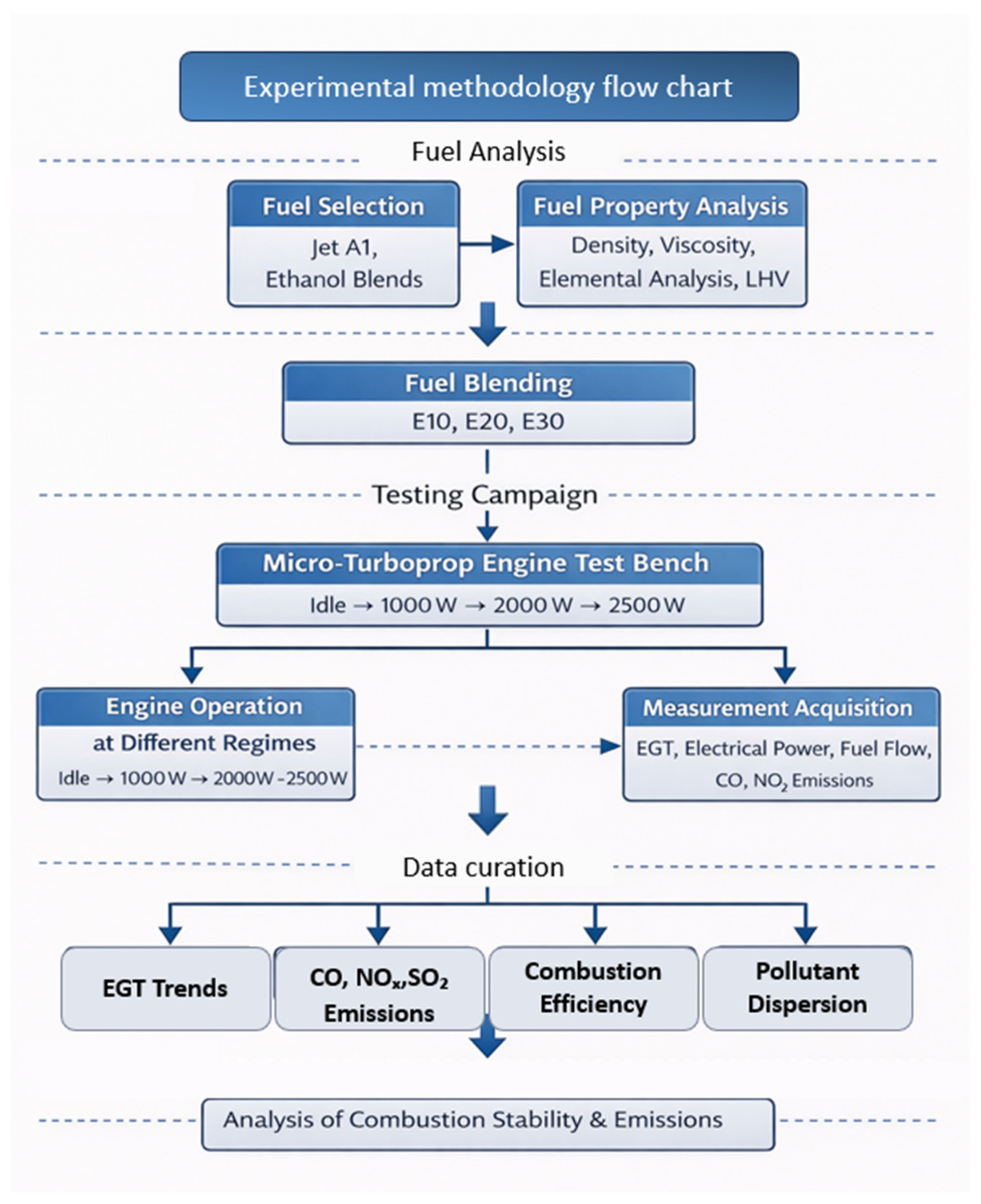
Figure 1. Experimental methodology flow chart.
Fuels 07 00022 g001
Figure 2. Component layout of the hybrid power source [32].
Fuels 07 00022 g002
Figure 3. The MRU GmbH Nova Plus monitoring system.
Fuels 07 00022 g003
Figure 4. The experimental setup.
Fuels 07 00022 g004
Figure 5. The evolution of the main pollutants based on wind speed and direction for E10 blend.
Fuels 07 00022 g005
Figure 6. The evolution of the main pollutants based on wind speed and direction for E20 blend.
Fuels 07 00022 g006
Figure 7. The evolution of the main pollutants based on wind speed and direction for E30 blend.
Fuels 07 00022 g007
Figure 8. The variation in the exhaust gas temperature across the four operating regimes.
Fuels 07 00022 g008
Figure 9. The variation in the CO across the four operating regimes.
Fuels 07 00022 g009
Figure 10. The variation in the NO across the four operating regimes.
Fuels 07 00022 g010
Figure 11. The variation in the SO2 across the four operating regimes.
Fuels 07 00022 g011
Figure 12. Approximation function.
Fuels 07 00022 g012
Figure 13. Comparative performance evaluation of ethanol–kerosene fuel blends and conventional kerosene.
Fuels 07 00022 g013
Figure 14. Final stage observations of combustion stability.
Fuels 07 00022 g014
Table 1. Physicochemical Properties of the ethanol–kerosene blends [20].
Sample Percentage [%]Flashpoint [K]Viscosity [cSt]Density [g/cm3]Calorific Power [MJ/kg]Elemental Analysis [%]
EthanolKerosene CHNO
010042.301.390.8245.2985.1713.310.071.45
100013.001.200.7929.4552.0913.020.0034.73
109023.701.370.8143.7181.8613.280.064.78
208023.601.350.8142.1278.5513.250.0611.43
307023.301.330.8140.5475.2513.110.0511.43
Table 2. Technical specifications of the test bench.
ParametersSpecifications
Engine ParametersMass1.8 kg
Conventional Fuel typeKerosene
(+5% Aeroshell Oil)
Maximum Rotational Speed170,000 rpm
Fuel Consumption Rate220 g/min
Test Bench ParametersMaximum Power Output3.5 kW
IDLE regime Voltage20 V
Nominal Operating Voltage48 V
Data acquisition Rate1 Hz
Table 3. Polynomial Coefficients for the Approximation Functions.
CoefficientEthanol 10%Ethanol 20%Ethanol 30%
A0−1.83563676 × 10−92.96927515 × 10−11−3.11524073 × 10⁻¹⁰
A14.41720336 × 10−7−1.19320864 × 10−81.05616252 × 10−7
A2−3.34564524 × 10−51.81570272 × 10−6−1.49050881 × 10⁻⁵
A33.17500750 × 10−4−1.28265582 × 10−41.14188131 × 10−3
A46.66772921 × 10−23.76509335 × 10⁻³−5.19156789 × 10⁻²
A5−2.221392035.65588167 × 10−31.42802971 × 10
A61.98530009 × 10−1.84522487−2.2200001 × 10
A702.0113672 × 101.66570353 × 102
A800−3.9029482 × 10²
Disclaimer/Publisher’s Note: The statements, opinions and data contained in all publications are solely those of the individual author(s) and contributor(s) and not of MDPI and/or the editor(s). MDPI and/or the editor(s) disclaim responsibility for any injury to people or property resulting from any ideas, methods, instructions or products referred to in the content.