Experimental Studies on Wood Pellets Combustion in a Fixed Bed Combustor Using Taguchi Method

Abstract

The combustion of wood pellets in a fixed bed combustor of a 20 kW capacity domestic pellet boiler was tested according to several factors including Power, Excess Air (EA), Primary/Secondary air Split Ratio (SR) and Grate Area (GA). The Taguchi method was applied to program the experimental design. Several parameters were measured, including gas emissions (CO), fuel bed temperature (measured at 4 different heights), and efficiency. The experimental results show that the lower CO emission and the higher efficiency were obtained at medium thermal loads and the highest temperature on the fuel bed was obtained at about ¼ of its height (15 mm). The results obtained from the analysis of variance (ANOVA) show that the SR and the Power are the most important factors contributing to the CO reduction and also increase the fuel bed temperature.

1. Introduction

Biomass is one of the renewable resources that contributes to the energy mix, reducing the negative impact on the environment, creating more jobs, among other factors [1,2]. With the goal of decreasing the share of fossil fuels and its contribution to climate change, developing technologies to efficiently convert energy from the renewable sources is a sustainable manner to mitigate the problem [3,4,5]. World consumption of energy has increased gradually due to population growth and to technological development [6,7].

The highest efficiency registered on the combustion of biomass generally corresponds to the lowest CO emissions, a behaviour that can be explained by the complete oxidation of the hydrocarbons contained on the wood [8,9]. The complete combustion is determined by several factors that can be summarized as good mixing and adequate residence time at high temperatures [8].

Various studies have been conducted in order to establish good methods in how to achieve a high combustion efficiency using biomass resources. Such high efficiency of biomass/waste combustion was obtained from advanced grate-firing [10]. Other studies also report that the boiler efficiency is also determined by the load factor and number of ignitions [11], suggesting that high operational loads and reduced number of ignitions correspond to the optimal operating conditions. Four appliances with different designs and several fuel types were investigated by Kinsey et al. [12]. Among these appliances the thermal, and combustion efficiencies, along with CO, CO₂ and other gas emissions were observed. The results showed that the four units corresponding to the tested pellet-burning appliances had the highest overall operating efficiency and lowest emissions.

On the other hand, accumulated ash on fixed grate biomass pellet boilers can sinter, imposing deficiencies on air supply and, thus, cause a poor combustion, with high CO emission. Although this phenomenon is linked to the mineral composition of the ash, it can be mitigated by controlling fuel bed temperature and primary/secondary air split ratio [13].

Applying different operating parameters in a wood pellets boiler, one can determine the combustion behaviour and overall performance of the boiler. Nonetheless, the boiler needs to be operated in an optimum way to improve its efficiency and lower the pollutant gas emission. The aim of this study was to investigate the influence of the thermal load, primary/secondary air split ratio, grate area and excess air on the gases of wood pellet combustion in a domestic boiler with a nominal power of 20 kW. The Taguchi method was applied to set the research plan and a statistical analysis (ANOVA) was performed to evaluate the results.

The Taguchi method is an approach for industrial product design built on statistically designed experiments. The key of this method is the parameter design, allowing the study of the influence of several factors in one or more parameters [14].

Several authors have used the Taguchi method to study the combustion or pre-treatment of biomass. As examples, Huang et al. [15] used the Taguchi method to optimize the torrefaction conditions for biochar cofiring. They concluded that the fuel characteristics were significantly influenced by the temperature, and to a less extent by the residence time and N₂ flow rate. Li et al. [16] applied the method to optimize the pre-treatment (torrefaction) of biomass to improve energy yield and heating value. Like Huang, Li concluded that the temperature was the major influencer on the torrefaction, followed by the residence time and the N₂ flow rate. On another work, Li et al. [17] used the method to optimize the combustion efficiency of a fluidized bed fed with torrefied biomass. They concluded that the degree of torrefaction of the biomaterials had the strongest influence on the total combustion efficiency, followed by the bed temperature and oxygen concentration with the same importance, and with less influence on the oxygen inlet.

According to the literature, the Taguchi method appears to be a suitable method to identify the influence of several factors on the performance of a process, and it has been used for optimizing the operational conditions. This method it is also known for the reduced number of tests needed to obtain conclusions and quantify the influence of the factors on the parameters, reducing time and resources. In this work, the Taguchi method was used to discover the parameters that have a major influence on gas emissions in order to optimize the combustion efficiency of a 20 kW boiler.

2. Materials and Methods

The experimental tests were realized using ENplus A1 Class standardized 6 mm diameter pine wood pellets [18]. Its relevant properties were measured and can be seen in

Table 1. Properties of pine wood pellets.

Analysis	Value (wt.%)
Proximate (as received)
Moisture	6.9
Volatile matter	77.8
Ash	0.6
Fixed carbon	14.7
Lower Heating Value (MJ/kg)	17.1
Ultimate (dry ash free)
Carbon (C)	50.8
Hydrogen (H)	5.4
Nitrogen (N)	1.6
Sulphur (S)	0.037
Oxygen (O)	42.2

.

The properties of the wood pellets were measured according to the norms:

• Moisture: EN ISO 18134:2015
• Volatile Matter: EN ISO 18123:2015
• Ash: EN ISO 18122:2015
• Low Heating Value: EN 14918:2009
• C, H, N: EN ISO 16948:2015
• Sulphur: EN ISO 16994:2016

The Fixed Carbon and the Oxygen were obtained by calculation, using the previous values. The fixed carbon was calculated following the Equation (1):

$$\mathrm{wt}.\%\mathrm{Fixed}\mathrm{Carbon}=100\%-\mathrm{wt}.\%\mathrm{Moisture}-\mathrm{wt}.\%\mathrm{Ash}-\mathrm{wt}.\%\mathrm{Volatile}\mathrm{Matter}$$

(1)

The Oxygen was calculated following the Equation (2):

$$\mathrm{wt}.\%\mathrm{O}=100\%-\mathrm{wt}.\%\mathrm{C}-\mathrm{wt}.\%\mathrm{H}-\mathrm{wt}.\%\mathrm{N}-\mathrm{wt}.\%\mathrm{S}$$

(2)

2.1. Experimental Setup

The experiment was conducted at the Heat and Fluids Laboratory of the Department of Mechanical Engineering of the University of Minho. A prototype, computer-controlled 20 kW domestic wood pellet boiler designed by a research team, was used. A representation of the experimental setup used in this study is presented in Figure 1. The pellets were transported from the pellets storage tank by means of a feeding auger and discharged through the top of the combustion chamber by gravity. A scale was placed under the pellet tank, allowing the measurement of the fuel consumption.

The boiler external dimensions were 127 cm height, 43 cm width and 35 cm depth. The combustion chamber was 53 cm in height and had a rectangular cross section of 30 × 25 cm. The combustion chamber was lined with 20 mm thick slabs of fire clay in order to avoid the formation of cold walls that would lower the combustion rates and may lead to incomplete combustion. Then, useful heat was transferred to water by means of double pass fire tube heat exchanger made up of 20 pipes inside the ±80 L water tank (Figure 2).

The burner was cantered at the bottom of the combustion chamber and comprised the grate and injectors for primary and secondary air supply. The bottom of the grate was covered by a metal box creating the ash pan and the primary air plenum. This assembly was put together with bolts and allowed us to easily change the grate. A sealing material (rock wool) was applied to the connection between the parts to prevent uncontrolled air leaks during operation. The primary air intake pipe was installed on an ash pan wall, along with the ignition coil. The upper section of the burner had a perforated surrounding collar, constituting the secondary air plenum.

The grate used in this study was of rectangular shape and three different cross sectional areas were tested (Figure 3).

The temperature on the fuel bed was measured using four type K thermocouples, installed at four different points/heights. A simple scheme of the fuel bed set is presented in Figure 2.

An air extractor, powered by an electric motor working at frequencies between 0 to 60 Hz, was located at the exhaust draft. This extractor forced the air to flow into the burner by the primary and secondary air ducts. The total air flow rate was set by adjusting the air extractor and the primary/secondary air split is adjusted by throttling the primary air supply. The whole unit was covered by a jacket of rock wool to minimize the heat losses to the outside.

A heat exchanger (Figure 1) was placed at the top of the boiler, enabling the produced heat to be removed from the boiler. Water was circulated using a pump (maximum flow rate of 500 L/h) that moved the water to an air-cooled heat exchanger. The flow rate was controlled by a valve and measured by a calibrated rotameter.

Finally, a vacuum pump was used to extract a sample of the flue gas into the gas analyser for measurement purposes. Before entering the vacuum pump, the sample was cooled and filtered in order to remove any moisture and particles.

A computer unit, composed of a National Instruments data acquisition system, was used as a data acquisition and control device. This system is divided in several parts, namely: a chassis (PXI-1052); controller (PCI-8105); acquisition board (PXI-6259); thermocouples module (SCXI-1102); analog inputs module (SCXI-1100); digital inputs module (SCXI-1326); and output digital module (SCXI-163) [20].

The controller works as a computer running Windows XP as the operative system. LabView was used to develop the interface and the boiler control program.

2.2. Test Procedure

Several factors were studied in this experiment including power (10, 13 and 16 kW), grate area (90 × 75, 115 × 75, and 115 × 96 mm²), excess air ratio (1.5, 1.7, and 2.1) and primary/secondary air split ratio (20/80, 30/70, and 37/67). The temperature at the centre of the fuel bed was measured at four different heights, namely 5, 15, 25 and 60 mm. The thermocouples were introduced from the bottom of the grate allowing the contact with the pellets.

With respect to the primary air, most of the air was introduced at the bottom of the grate through orifices of a rectangular shape (3 × 26 mm²), and some air was also introduced at the bottom side of the grate through orifices of 4 mm diameter (Figure 3). The number of orifices depended on the cross-sectional area of the grate. Regarding the secondary air, 12 orifices with a diameter of 4 mm were located at the top of the burner, in each side, 92 mm above the fuel bed.

To continuously measure the CO and O₂ composition of the flue gas, a Signal Instruments 9000MGA gas analyser was used, and the CO concentration was corrected to 13% of O₂. The equipment uses a parametric oxygen sensor with a repeatability of ±0.01% for the O₂ measurement and an infrared sensor with a repeatability better than ±1% or ±0.5 ppm for the CO and CO₂ measurement [21]. The sample gas cooling and conditioning system is presented in Figure 4. For each experiment the boiler was running for 4 h after a warmup period. The boiler was shut down if instabilities and irreversible build-up of pellets on the grate were observed. The temperature on both hot and cold water pipes was recorded in order to assess the removed thermal power and consequently allowing for boiler efficiency calculations.

The parameter that better describes the combustion quality is the CO emission. Meanwhile, during the long run tests, the CO concentration could fluctuate and increase significantly as the fuel bed (FB) rises. If that occurred, the CO emission considered in the study was the one registered before the occurrence of those instabilities in the FB.

2.3. Design of Experiments Using Taguchi Method

The application of the Taguchi method in the planning of experimental projects can significantly reduce the amount of tests required to evaluate the influence of several factors considered in a particular process [22]. In addition, this method also allows one to confirm the importance and relative weight of each factor in a particular response or outcome expected. The key of the Taguchi method is the parameter design [14].

In the Taguchi method, multiple parameters (factors) and several values of these parameters (factor levels) are arranged according to standard orthogonal arrays, enabling a dramatic decrease in full-factorial trial experiments [23]. As described by Ferreira [22], there are three phases in applying the method:

(1)

Selection of factors and eventual interaction;

(2)

Planning of the experiment; and

(3)

Analysis and interpretation of the results.

In addition, for the experimental plan, at least 3 levels on each parameter should be applied to evaluate the influence of each parameter. The value of the parameters and the three different levels for each selected parameter for this experiment are presented in

Table 2. Factor and Level of the experimental plan, using the Taguchi method.

Factor		Level
		1	2	3
A	Power (kW)	10	13	16
B	Excess air (%)	50	70	110
C	Grate area (mm2)	90 × 75	115 × 75	115 × 96
D	Split ratio (P/S)	20/80	30/70	37/63
Grate height 61 (mm)

. Based on this experimental plan, the test plan matrix to be used is the orthogonal matrix L27, which consists of 27 experiments and 13 columns (

Table 3. Matrix L₂₇, with indication parameter (1, 2, 5, 10), interaction (3, 4, 6, 7, 8, 11), and independent (9, 12, 13) [22].

Test	Power (kW)	EA (%)			GA (mm2)					SR
	A	B	A × B		C	A × C		B × C	e	D	B × C	e	e
	1	2	3	4	5	6	7	8	9	10	11	12	13
1	1	1	1	1	1	1	1	1	1	1	1	1	1
2	1	1	1	1	2	2	2	2	2	2	2	2	2
3	1	1	1	1	3	3	3	3	3	3	3	3	3
4	1	2	2	2	1	1	1	2	2	2	3	3	3
5	1	2	2	2	2	2	2	3	3	3	1	1	1
6	1	2	2	2	3	3	3	1	1	1	2	2	2
7	1	3	3	3	1	1	1	3	3	3	2	2	2
8	1	3	3	3	2	2	2	1	1	1	3	3	3
9	1	3	3	3	3	3	3	2	2	2	1	1	1
10	2	1	2	3	1	2	3	1	2	3	1	2	3
11	2	1	2	3	2	3	1	2	3	1	2	3	1
12	2	1	2	3	3	1	2	3	1	2	3	1	2
13	2	2	3	1	1	2	3	2	3	1	3	1	2
14	2	2	3	1	2	3	1	3	1	2	1	2	3
15	2	2	3	1	3	1	2	1	2	3	2	3	1
16	2	3	1	2	1	2	3	3	1	2	2	3	1
17	2	3	1	2	2	3	1	1	2	3	3	1	2
18	2	3	1	2	3	1	2	2	3	1	1	2	3
19	3	1	3	2	1	3	2	1	3	2	1	3	2
20	3	1	3	2	2	1	3	2	1	3	2	1	3
21	3	1	3	2	3	2	1	3	2	1	3	2	1
22	3	2	1	3	1	3	2	2	1	3	3	2	1
23	3	2	1	3	2	1	3	3	2	1	1	1	2
24	3	2	1	3	3	2	1	1	3	2	2	3	3
25	3	3	2	1	1	3	2	3	2	1	2	1	3
26	3	3	2	1	2	1	3	1	3	2	3	2	1
27	3	3	2	1	3	2	1	2	1	3	1	3	2

).

The notation of a Taguchi orthogonal array can be written as L27 (313). In this notation, 27 is the number of the experimental runs, 3 is the number of levels and 13 is the number of experimental factors. Furthermore, the L27 matrix with 13 columns can be used for the study of seven factors and three interactions, where each interaction requires two columns (see Table 3) [22].

According to Ferreira [22], for the optimization process, the deviation to the optimal value depends on the dispersion of results. Thus, the analysis of variance (ANOVA) is based on the mean and variance of each test. ANOVA provides the dispersion present in a specific set of data, identifying their origins and evaluating the contribution of each data point to the total dispersion. This method allows for the testing of the significance of the effects relative to the random error, also known as noise. The data obtained from the experiment was transformed into a signal-to-noise ratio (S/N) to measure the deviation of quality of the parameters from the desired values. The S/N ratio is always <0. A higher value ratio corresponds to a better quality characteristic of the observed parameter. Thus, values close to zero indicate the best conditions [24,25]. In the Taguchi method, three types of characteristic performance are selected in the analysis, including the-larger-the-better, the-smaller-the-better, and the-nominal-the-better (on-target-better) [23,24].

For the analysis of variance for CO, the-smaller-the-better was selected for the calculation of S/N Equation (3) [22]:

$$\mathrm{S}/\mathrm{N}=-10\log ({\overline{X}}^2+{{\sigma }_x}^2)$$

(3)

And for temperature, the-nominal-the-better was selected, represented by the Equation (4):

$$\mathrm{S}/\mathrm{N}=-10\log \left({{\sigma }_x}^2\right)$$

(4)

where ${\overline{X}}^2$ is the average value of the data and ${{\sigma }_x}^2$ is the variance.

The boiler efficiency was calculated according to the NF EN 303-5 standard following Equation (5) [26]:

$${\eta }_b=100\frac{P_n}{P_i}$$

(5)

where $P_n$ is the nominal useful power of the boiler (kW) that was calculated by Equation (6):

$$P_n=\dot{m_w}{C}_{pw}{\Delta T}_w$$

(6)

where $\dot{m_w}$ is the water mass flow rate (kg⋅s⁻¹), $C_{pw}$ is the heat capacity of water (kJ⋅kg⁻¹⋅K⁻¹) and ${\Delta T}_w$ is the temperature difference between the boiler and the heat exchanger.

$P_i$ is the power input and can be calculated as (Equation (7)):

$$P_i=\dot{ m_f}{LHV}_f$$

(7)

where $\dot{m_f}$ is the mass flow rate of the fuel (kg⋅s⁻¹) and the ${LHV}_{\mathrm{f}}$ is the Low Heating Value of the fuel (kJ⋅kg⁻¹).

3. Results and Discussion

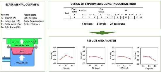
Considering four factors and three levels, in a normal matrix it would be necessary for 81 tests (without interactions) to perform all the combinations. The implementation of the Taguchi method allowed the reduction to 27 tests and added interactions and external factors to the matrix, substantially reducing the cost and time needed to understand the interaction between factors.

The statistical analysis (ANOVA) from the Taguchi method gives a better understanding on the influence of each parameter, which is important to understand and optimize the process.

For all the 27 tests, the overall efficiency of the boiler varied between 64% and 92% with an average of 83%.

Figure 5 depicts the relationship between GA and thermal efficiency at different power, SR, and EA. Figure 5a shows that at 10 kW with 50% of EA (EA1), the efficiency was higher for the combination of middle GA (GA2) with middle SR (SR2). For 70% of EA (middle EA: EA2), the best combination was found using the middle GA (GA2), but with higher SR (SR3). As for an EA of 110% (EA3), it was noted that the thermal efficiency was higher for both the combination of smaller GA (GA1) with SR3 and larger GA (GA3) with middle SR (SR2).

In brief, Figure 5a shows that at low power (10 kW), the best combination of the parameters is either EA3-GA1-SR3 or EA3-GA3-SR2 in order to obtain the higher combustion efficiency. This means that lower power conditions require a high EA. The reduced efficiency at lower thermal loads may be due to the size of the combustion chamber, which will require a higher EA to provide adequate mixing with the fuel. The opposite may be observed for higher power levels (see Figure 5c).

Figure 5b shows the results for the 13 kW load. It can be observed that at 50% of EA the thermal efficiency was higher for both the combination of smaller GA (GA1) with SR3 and larger GA (GA3) with middle SR (SR2). For 70% of EA (EA2), the combination of GA1 with lower SR (SR1) and GA3 with higher SR (SR3) presented the highest thermal efficiencies. For 110% of EA, the thermal efficiency was slightly higher for GA1 and GA2, with the combination with SR2 and SR3, respectively. These results show that, at medium power (13 kW), the best combination of the parameters is either EA2-GA1-SR1 or EA2-GA3-SR3 in order to produce the highest thermal efficiency.

Figure 5c depicts the results for the 16 kW load. In this condition, for 50% of EA, the thermal efficiency was higher at middle GA (GA2) combined with SR3. For 110% of EA (EA3), the maximum efficiency occurred at the combination of GA2 with middle SR (SR2). For 70% of EA, the thermal efficiency was higher for the combination of GA3 with SR2. Globally, this analysis shows that the best combination of the parameters was EA1-GA2-SR3. This means that at a higher power level, a lower EA and middle GA with higher SR most likely result in high thermal efficiency.

Overall, the data in Figure 5 indicate that an efficient combustion can be obtained with any grate, once the EA and SR are properly adjusted for any specific power level. This is in line with the results obtained from Verma et al. [27]. High efficiencies usually cannot be obtained at high EA due to thermal stack losses, as stated by Serrano et al. [28]. On the other hand, high CO emission can also induce low efficiencies because this condition shows, basically, that some fuel was left unburned. At low power levels, increasing excess air promotes a better air/fuel mixing and higher carbon conversion which decreases CO emissions. So, the efficiency of the boiler is a compromise between thermal and chemical losses on the stack [29]. This can explain the higher level of excess air required at low power level to guarantee maximum efficiency.

3.1. ANOVA Analysis of CO Emissions

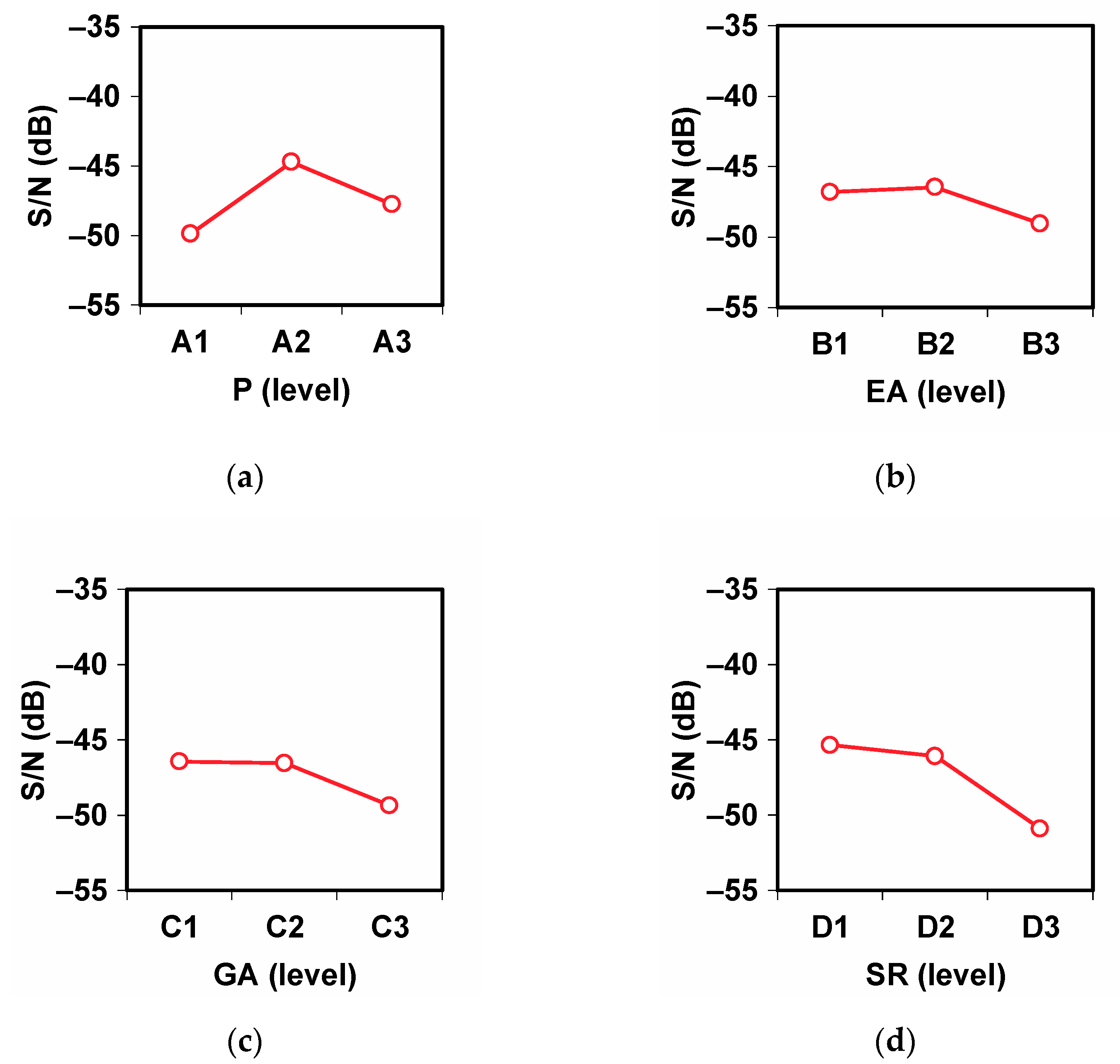
The mean values of the S/N indices for each of the three levels of each parameter or interaction on CO are presented in

Table 4. Mean values of S/N index and maximum differences between levels on CO.

	P	EA			GA					SR
S/N	A	B	A × B		C	A × C		B × C	e	D	B × C	e	e
1	−49.9	−46.8	−48.7	−49.2	−46.4	−47.0	−48.6	−47.4	−47.2	−45.3	−48.2	−48.0	−48.6
2	−44.7	−46.5	−46.1	−46.7	−46.5	−46.3	−47.4	−46.5	−45.9	−46.1	−46.2	−47.1	−46.1
3	−47.8	−49.1	−47.5	−46.4	−49.6	−49.0	−46.3	−48.4	−49.2	−50.9	−47.9	−47.2	−47.6
dif.	5.2	2.6	3.1		2.9	2.7		2.2	3.3	5.6	-	0.8	2.5

. The last line of each table shows the maximum value of the difference between the averages of the indices for each of the parameters. These results evaluate the relative weight of the influence of each parameter on the response value. Based on its analysis, it can be verified that the split ratio (SR) index (parameter D, dif. = 5.6) has the highest contribution to CO reduction, followed by parameter A (power, dif. = 5.2), the interaction of parameters power and EA (dif. = 3.1), parameter C (GA, dif. = 2.9) and parameter B (EA, dif. = 2.6). There is a parameter that was not identified, whose influence is higher than that of the interaction of parameters power and EA, GA, and EA. This indication is supported by the value of the left-hand column of the SR value (column 10 is identified as “e”) and presents a dif. = 3.3. This result may show the influence of parameters that were not considered but make some significant contribution to the process, for example the combustion chamber temperature.

Table 5. Analysis of the relative contribution of the parameters based on the mean concentration of CO.

	P	EA			GA					SR
Average	A	B	A × B		C	A × C		B × C	e	D	B × C	e	e
1	376.8	285.8	333.5	349.0	240.1	246.7	290.4	245.4	249.3	198.6	284.5	272.4	288.5
2	182.7	231.8	230.1	228.5	229.1	232.8	247.8	236.0	211.6	212.6	220.6	245.5	233.5
3	256.9	298.9	252.9	239.0	347.2	337.0	278.2	335.1	355.5	405.3	311.4	298.6	294.4
dif.	194.1	67.2	120.5		118.2	104.2		114.5	143.9	206.7		53.1	60.9

presents the analysis based only on the mean values of the CO concentration for each parameter. These data confirm the trend observed by the analysis of the S/N indices, on how to minimize the response value. It shows that the most important is SR, with a difference of about 207 ppm, followed by power at 194 ppm, and other unidentified parameters (column 9 is identified as “e”) at 144 ppm.

Figure 6 shows the dependence of the response value with the different parameters, for the various levels of analysis. These data show the evolution through the three levels for each of the parameters with respect to the CO concentration. Figure 6a shows that the lowest observed CO emission occurs at medium power (13 kW). Meanwhile, Figure 6b–d demonstrates that CO emission is lower at the lower level of the parameter applied and increases with the increasing of the EA, GA, and SR, respectively. This means that an isolated increase of any one of those parameters creates more unburned substances, translating into a rise in CO emissions.

Figure 7 presents the interaction between all parameters on CO emission. From its analysis one can identify that there is an important interaction between middle power and lower EA (Figure 7a), and between middle power and lower GA (Figure 7b). Based on Figure 7 and the value of maximum differences between levels on CO (Figure 6), we can conclude that the best combination to reduce the variance (more stable and best result) is A2-B1-C1-D1, corresponding to middle power, at low excess air, small grate area and low split ratio.

For the analysis of variance (ANOVA), an F-test was performed. On an F-test, the F value corresponds to a ratio between the variance of a parameter and the variance of the error.

Table 6. ANOVA analysis.

ANOVA	P	EA		GA				SR			Error Calculation
	1	2	3 & 4	5	6 & 7	8 & 11	9	10	12	13
	A	B	A × B	C	A × C	B × C	e	D	e	e	Error Exp.	Total
df	2	2	4	2	4	4	2	2	2	2	22	26
sq	121.14	35.84	73.10	49.06	60.09	36.08	50.35	163.76	3.74	27.84	336.09	620.99
var	60.57	17.92	18.28	24.53	15.02	9.02	25.18	81.88	1.87	13.92	15.28	23.88
pool	n	s	s	s	s	s	s	n	s	s	n	-
F	3.96	-	-	-	-	-	-	5.36	-	-	-	-
sq’	90.59	-	-	-	-	-	-	133.20	-	-	397.20	620.99
%	14.59	-	-	-	-	-	-	21.45	-	-	63.96	100.00

shows the results of the F-test from the analysis of variance. To determine whether an F value of two variances is statistically high, one should consider: (i) the level of confidence required; (ii) the degrees of freedom associated with the variance of the sample in the numerator; and (iii) the degrees of freedom (df) associated with the sample variance in the denominator. The critical value of F is then compared with the F value of a ratio of sample variances. The analysis of variance is a more objective and quantifiable test, allowing conclusions which are not possible with the simple analysis of the means or the S/N indices.

Table 7. ANOVA F critic calculation for CO.

F Critic
	Degree of Freedom (df)
Nominator	2	4
Denominator	22	22
$\alpha$
0.10	2.56	2.22
0.05	3.44	2.82
0.01	5.72	4.31

presents the statistical calculation of the F critical according to the level of risk $\mathsf{\alpha }$ (1%, 5%, and 10%), for the final configuration of Table 6. This method of analysis was previously applied by Ferreira [22].

In Table 6, only the parameters that contribute significantly to the reduction of CO concentration are identified. After applying the analysis of variance, from Table 6, it is observed that the F value associated to parameter D (SR) is higher than the critical value for the confidence index (risk $\mathsf{\alpha }$= 0.05) but less than $\mathsf{\alpha }$ = 0.01, calculated for the same number of degrees of freedom (df = 2). From these results, one can conclude that, with a confidence index higher than 95%, it can be stated that the SR intensity contributes by about 21% to the reduction of CO concentration. The same scenario occurs for the F value associated with power, which is higher than the value for $\mathsf{\alpha }$ = 0.05. This means that the confidence index is the same as the previous parameter referred to the SR. Based on that, it can be said that, with a confidence index of over 95%, the influence of power contributes approximately 15% to the reduction of CO concentration.

Looking at Table 6, one can conclude that the main effect comes from the SR followed by power (A). However, the value associated with the experimental error is 63.96%. This value is indeed significant and deserves careful consideration, as it has a dimension to mask the influence of the most significant parameters. In practice, this error can be the result of several factors: an important parameter not considered in the study, unsuitability of the selected levels, misadjustment with the level of factors, and any deficiency in the control of the chosen parameters or instabilities in the operation, as stated by Ferreira [22].

3.2. ANOVA Analysis on Temperature

The mean values of the S/N indices for each of the three levels of all parameters or interaction with fuel bed temperature are presented in

Table 8. Mean values of the S/N index and maximum differences between levels on temperature.

	P	EA		GA				SR
S/N	A	B	A × B	C	A × C	B × C	e	D	e	e
dif. (5 mm)	4.22	4.55	2.78	2.76	1.61	2.16	0.75	3.70	2.14	0.59
dif. (15 mm)	2.42	2.27	3.13	1.67	2.51	4.25	4.08	4.21	2.10	3.77
dif. (25 mm)	2.64	2.01	6.60	5.66	4.08	2.67	3.95	7.91	3.98	2.65
dif. (60 mm)	2.97	0.90	4.43	4.42	1.80	3.36	1.31	4.95	3.96	1.21

. The data show the maximum value of the difference between the averages of the indices for each of the parameters. These results evaluate the relative weight of influence of each parameter on the response value.

Table 8 presents the mean value of the S/N index and the maximum difference between levels on the temperature at different heights in the fuel bed. For temperatures at 5 mm, the excess air (EA) has the highest contribution to increasing the temperature, followed by power, SR, the interaction of parameters power and EA, and the parameter GA. For temperatures at 15 mm, the highest contribution is the interaction of parameters EA and GA, SR, and one unidentified parameter (column 10) followed by another unidentified parameter (column 14), the interaction of power and EA, and power and GA. For temperatures at 25 mm, the highest contribution is from the parameter SR, followed by interaction of parameters power and EA, GA, the interaction of power and GA, and two unidentified parameters (column 13 and 10). For temperatures at 60 mm, the highest contribution is from parameter SR, followed by interaction of parameters power and EA, GA, one unidentified parameter (column 13), and the interaction of EA and GA.

The temperature behaviour on the fuel bed at 5, 15, 25, and 60 mm was also studied.

Table 9. Analysis of the relative contribution of the parameters on the mean temperature.

	P	EA		GA				SR
Average	A	B	A × B	C	A × C	B × C	e	D	e	e
dif. (5 mm)	1.7	47.1	18.1	52.6	43.3	34.9	43.5	55.1	5.5	23.0
dif. (15 mm)	108.4	33.5	54.1	72.3	49.5	42.4	73.8	38.4	49.1	31.4
dif. (25 mm)	102.4	10.8	70.6	102.2	69.9	67.2	51.1	51.3	63.2	39.4
dif. (60 mm)	110.3	44.4	34.2	142.9	61.2	104.5	41.6	87.2	31.0	20.6

presents the analysis based only on the mean values of temperature at 5, 15, 25, and 60 mm observed for each parameter. The data confirms the trend observed by the analysis of the S/N indices.

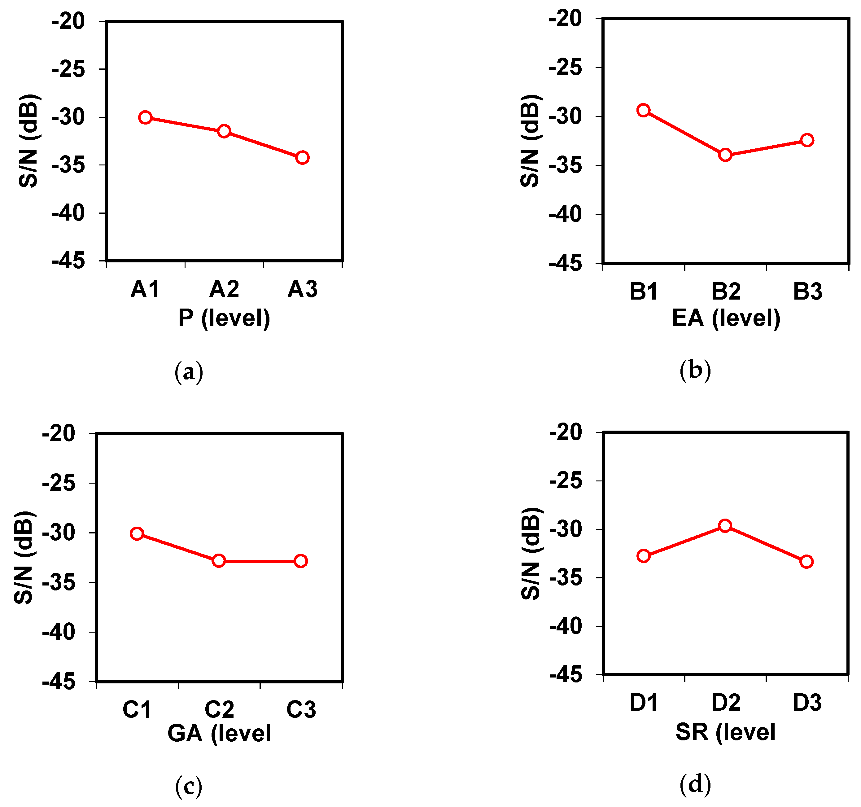
Figure 8 shows the evolution of S/N for temperature at 5 mm height with the different parameters, for the various levels of analysis. The temperature decreases as power increases, a behaviour that may result from the accumulation of wood pellets on the burner at high power levels, moving away the reaction zone from the grate. The parameters EA and GA present almost the same behaviour, showing that lower power levels yield higher temperatures. This phenomenon can be explained by the fact that higher EA and GA provide more air into the grate that may reduce the temperature. For SR, the higher temperature was observed at the middle set point, a situation that may represent the competition between two effects: a temperature increase as a result of the heat generated by higher devolatilization that occurs with increasing primary air and the cooling effect of a greater air mass crossing the fuel bed.

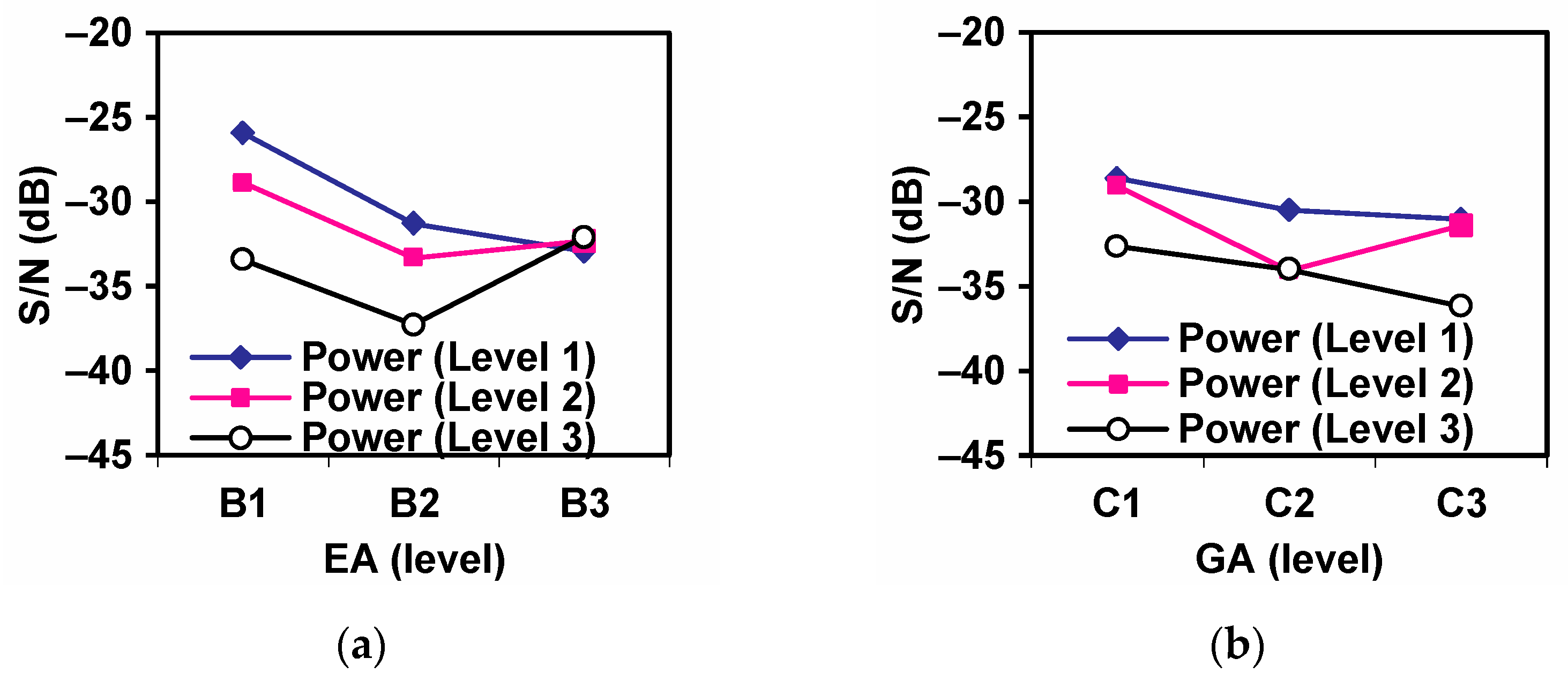
Figure 9 presents the interaction between all parameters for the temperature at 5 mm. From these graphs it can identified that there is an important interaction between lower power and lower EA (Figure 9a), and between lower power and lower GA (Figure 9b). Based on Figure 9 and the value of maximum differences between levels on temperature at 5 mm (Table 8), the best combination to reduce the variance (more stable and best result) is A1-B1-C1-D2, corresponding to low power level, low excess air, low grate area and intermediate split ratio.

Table 10. The overall influences of the parameters on fuel bed temperature.

Height (mm)	P	EA		GA				SR
	A	B	A × B	C	A × C	B × C	e	D	e	e
	1	2	3 & 4	5	6 & 7	8 & 11	9	10	12	13
5	14.4%	17.6%	-	-	-	-	-	11.8%	-	-
15	-	-	-	-	-	-	-	-	-	-
25	-	-	-	-	-	-	-	21.0%	-	-
60	5.0%	-	17.2%	17.2%	-	9.3%	-	19.2%	12.8%	-

presents the overall influences of the parameters applied in this study on the fuel bed temperature at different heights. The data show that the most influencing parameter on the temperature at different heights is the SR, which is contributing about 12%, 21%, and 19% at 5, 25, and 60 mm respectively. The second parameter that most influences the temperature is power, which contributes approximately 14% and 5% at 5 and 60 mm.

4. Conclusions

The main purpose of this work was to study the influence of the thermal load, primary/secondary air split ratio, grate area and excess air on the gases of wood pellet combustion in a purpose-built wood pellet boiler by using the Taguchi method. The boiler was designed by a research team and was computer-controlled, capable of changing the fuel rate, air flow, primary-secondary air split ratio and the dimensions of the fuel grate.

The Taguchi method was applied in order to optimize the process. It has been used by other authors and is considered one of the most efficient in the field. The Taguchi method allows one to comprehend the interaction and the influence of factors in order to optimize the process. At the same time, due to its simplicity, it allows the reduction of the total number of tests, reducing time and cost.

The highest thermal efficiency obtained was 92%. This efficiency corresponded to the lowest CO emissions, and it was obtained at middle power, middle excess air (EA), higher split ratio (SR) and higher grate area (GR).

From the Taguchi method and the statistical analysis (ANOVA), it was concluded that the split ratio was the parameter contributing the most for the CO reduction on a percentage of 21.5%, followed by power with 14.6%. The data show that the medium power level (13 kW) has the highest efficiency and lowest CO emissions compared to both lower (10 kW) and higher power (16 kW). The excess air (EA), grate area (GA), and SR show the same trend for the efficiency and CO emissions, where lower and middle values for those parameters correspond to optimal performances.

Regarding the average temperature in the fuel bed, the results indicated that the highest temperature was observed at 15 mm followed by 25, 5 and 60 mm in height. The SR and power levels are the most important parameters contributing to increase the fuel bed temperature.

References

1. Gonzaga Fraga, L.; Carlos, F.; Teixeira, J.; Eduardo, C.; Ferreira, M. The Potential of Renewable Energy in Timor-Leste: An Assessment for Biomass. Energies 2019, 12, 1441. [Google Scholar] [CrossRef] [Green Version]
2. Nunes, L.J.R.; Matias, J.C.O.; Catalão, J.P.S. Biomass combustion systems: A review on the physical and chemical properties of the ashes. Renew. Sustain. Energy Rev. 2016, 53, 235–242. [Google Scholar] [CrossRef]
3. Shan, F.; Lin, Q.; Zhou, K.; Wu, Y.; Fu, W.; Zhang, P.; Song, L.; Shao, C.; Yi, B. An experimental study of ignition and combustion of single biomass pellets in air and oxy-fuel. Fuel 2017, 188, 277–284. [Google Scholar] [CrossRef]
4. Roy, M.M.; Dutta, A.; Corscadden, K. An experimental study of combustion and emissions of biomass pellets in a prototype pellet furnace. Appl. Energy 2013, 108, 298–307. [Google Scholar] [CrossRef]
5. Unpinit, T.; Poblarp, T.; Sailoon, N.; Wongwicha, P.; Thabuot, M. Fuel Properties of Bio-Pellets Produced from Selected Materials under Various Compacting Pressure. Energy Procedia 2015, 79, 657–662. [Google Scholar] [CrossRef] [Green Version]
6. Magelli, F.; Boucher, K.; Bi, H.T.; Melin, S.; Bonoli, A. An environmental impact assessment of exported wood pellets from Canada to Europe. Biomass Bioenergy 2009, 33, 434–441. [Google Scholar] [CrossRef]
7. Kruggel-Emden, H.; Wirtz, S.; Scherer, V. An experimental investigation of mixing of wood pellets on a forward acting grate in discontinuous operation. Chem. Eng. Sci. 2013, 233, 261–277. [Google Scholar] [CrossRef]
8. Olsson, M. Residential Biomass Combustion—Emissions Of Organic Compounds To Air From Wood Pellets And Other New Alternatives; Chalmers University of Technology: Gothenburg, Sweden, 2006. [Google Scholar]
9. González, J.F.; Ledesma, B.; Alkassir, A.; González, J. Study of the influence of the composition of several biomass pellets on the drying process. Biomass Bioenergy 2011, 35, 4399–4406. [Google Scholar] [CrossRef]
10. Yin, C.; Li, S. Advancing grate-firing for greater environmental impacts and efficiency for decentralized biomass/wastes combustion. Energy Procedia 2017, 120, 373–379. [Google Scholar] [CrossRef]
11. Carlon, E.; Schwarz, M.; Golicza, L.; Verma, V.K.; Prada, A.; Baratieri, M.; Haslinger, W.; Schmidl, C. Efficiency and operational behaviour of small-scale pellet boilers installed in residential buildings. Appl. Energy 2015, 155, 854–865. [Google Scholar] [CrossRef]
12. Kinsey, J.S.; Touati, A.; Yelverton, T.L.B.; Aurell, J.; Cho, S.H.; Linak, W.P.; Gullett, B.K. Emissions characterization of residential wood-fired hydronic heater technologies. Atmos. Environ. 2012, 63, 239–249. [Google Scholar] [CrossRef]
13. Ribeiro, P.; Teixeira, J.; Ferreira, M.E. Ash Sintering in A Biomass Pellet Boiler. In Proceedings of the ASME International Mechanical Engineering Congress and Exposition, San Diego, CA, USA, 15–21 November 2013; pp. 1–7. [Google Scholar] [CrossRef]
14. Simpson, T.W.; Peplinski, J.D.; Koch, P.N.; Allen, J.K. Metamodels for computer-based engineering design: Survey and recommendations. Eng. Comput. 2001, 17, 129–150. [Google Scholar] [CrossRef] [Green Version]
15. Huang, C.W.; Li, Y.H.; Xiao, K.L.; Lasek, J. Cofiring characteristics of coal blended with torrefied Miscanthus biochar optimized with three Taguchi indexes. Energy 2019, 172, 566–579. [Google Scholar] [CrossRef]
16. Li, Y.H.; Lin, H.T.; Xiao, K.L.; Lasek, J. Combustion behavior of coal pellets blended with Miscanthus biochar. Energy 2018, 163, 180–190. [Google Scholar] [CrossRef]
17. Li, Y.H.; Kuo, W.C. The study of optimal parameters of oxygen-enriched combustion in fluidized bed with optimal torrefied woody waste. Int. J. Energy Res. 2020, 44, 7416–7434. [Google Scholar] [CrossRef]
18. European Pellet Council ENplus Quality Certification Scheme Part 3: Pellet Quality Requirements. ENplus Handbook (UK Pellet Council-Handbook). 2015, pp. 0–10. Available online: https://enplus-pellets.eu/en-in/?option=com_attachments&task=download&id=145:ENplusHandbook_part3_V3 (accessed on 24 September 2019).
19. Fraga, L.G. Wood Pellets Combustion in a Fixed Bed Combustor. Ph.D. Thesis, University of Minho, Guimarães, Portugal, 2019. [Google Scholar]
20. Ribeiro, P.E.A. Aglomeração de Cinzas numa Caldeira a Pellets—Influência da Temperatura e do Fluxo de Ar. Master’s Thesis, University of Minho, Guimarães, Portugal, 2012. [Google Scholar]
21. Limited, S.G. 9000MGA—Multi Gas Analyser Operatig Manual; Signal Group Limited: Camberley Surrey, UK, 2003. [Google Scholar]
22. Ferreira, M.E.C. Atomização Efervescente na Combustão de Óleos Usados. Ph.D. Thesis, University of Minho, Braga, Portugal, 2008. [Google Scholar]
23. Liu, X.; Zhou, Y.; Li, C.-Q.; Lin, Y.; Yang, W.; Zhang, G. Optimization of a New Phase Change Material Integrated Photovoltaic/Thermal Panel with The Active Cooling Technique Using Taguchi Method. Energies 2019, 12, 1022. [Google Scholar] [CrossRef] [Green Version]
24. Thanakiatkrai, P.; Welch, L. Using the Taguchi method for rapid quantitative PCR optimization with SYBR Green I. Int. J. Legal Med. 2012, 126, 161–165. [Google Scholar] [CrossRef] [PubMed]
25. Babu, J.; Dutta, A.; Kumaraswamy, A. Experimental Studies on Effect of Temperature and Strain Rate on Deformation Behaviour of Ti-6Al-4V Using Taguchi Method. Procedia Mater. Sci. 2014, 6, 1121–1130. [Google Scholar] [CrossRef] [Green Version]
26. Lajili, M.; Jeguirim, M.; Kraiem, N.; Limousy, L. Performance of a household boiler fed with agropellets blended from olive mill solid waste and pine sawdust. Fuel 2015, 153, 431–436. [Google Scholar] [CrossRef]
27. Verma, V.K.; Bram, S.; Delattin, F.; De Ruyck, J. Real life performance of domestic pellet boiler technologies as a function of operational loads: A case study of Belgium. Appl. Energy 2013, 101, 357–362. [Google Scholar] [CrossRef]
28. Serrano, C.; Portero, H.; Monedero, E. Pine chips combustion in a 50 kW domestic biomass boiler. Fuel 2013, 111, 564–573. [Google Scholar] [CrossRef]
29. Arranz, J.I.; Miranda, M.T.; Montero, I.; Sepúlveda, F.J.; Rojas, C.V. Characterization and combustion behaviour of commercial and experimental wood pellets in South West Europe. Fuel 2015, 142, 199–207. [Google Scholar] [CrossRef]
Figure 1. Test facility setup: 1. Pellets hopper; 2. Feeding gauger; 3. Feeding gauger driver; 4. Scale; 5. Burner grate; 6. Primary air duct; 7. Secondary air duct; 8. Circulating water pump; 9. Flow meter; 10. Expansion vessel; 11. Water cooling unit; 12. Air Extractor; 13. Stack; 14. Flue gas probe to analyser.
Fuels 02 00022 g001
Figure 2. Boiler unit and Fuel Bed representation, adapted from [19]: 1. Primary air duct; 2. Secondary air duct; 3. Fuel Inlet; 4. Ignition Coil; 5. Fire Clay Slabs; 6. Grate; 7. Stack; 8. Heat Exchanger; 9. Fuel Bed; 10–13. Type K Thermocouples at 5, 15, 25 and 60 mm height, respectively.
Fuels 02 00022 g002
Figure 3. Grate Unit: 1–2. Primary air orifices; 3. Ignition hole; 4. Secondary air orifice; 5. Secondary air inlet 6. Bottom Grate.
Fuels 02 00022 g003
Figure 4. Flue gas analyser scheme: 1. Gas analyser; 2. Data acquisition system; 3. Cooling loop; 4. Filter; 5. Vacuum pump; 6. Water inlet.
Fuels 02 00022 g004
Figure 5. Relationship between efficiency and GA with different EA and SR: (a) at 10 kW, (b) at 13 kW, and (c) at 16 kW.
Fuels 02 00022 g005
Figure 6. Individual influence of factors on the response (CO) S/N obtained for the three leves of (a) Power (b) Excess Air (c) Grate Area (d) Split Ratio.
Fuels 02 00022 g006
Figure 7. Indices of interaction between factors on CO S/N values for: (a) each EA level at different power levels; (b) each GA level at different power levels.
Fuels 02 00022 g007
Figure 8. Individual influence of factors on the temperature at 5 mm, S/N obtained for the three leves of (a) Power (b) Excess Air (c) Grate Area (d) Split Ratio.
Fuels 02 00022 g008
Figure 9. Indices of interaction between factors (T at 5 mm) S/N values for: (a) each EA level at different power levels; (b) each GA level at different power levels.
Fuels 02 00022 g009