Three-Dimensional Reconstruction of Evaporation-Induced Instabilities Using Volumetric Scanning Particle Image Velocimetry

Abstract

The three-dimensional (3D) flow below the interface of an evaporating liquid at a low pressure is visualized and quantified using scanning particle image velocimetry. The technique presented highlights the use of a single camera and a relatively fast moving laser sheet to image the flow for an application where using more than one camera is difficult. The technique allows collection of the full three-dimensional velocity vector map over the whole liquid volume. The out-of-plane component of the velocity has been determined using two different processing approaches: (i) deriving the full vector from a 3D cross-correlation of the particle volumes and (ii) applying the continuity equation to determine out-of-plane velocities from the calculated in-plane velocity vector fields. The results obtained from both methods showed good agreement with each other. The 3D velocity field reveals the existence of a torus shaped vortex below the evaporating meniscus that was induced by the exposure of the cold liquid to the warmer solid walls. The velocity data also shows that the maximum velocity occurs below the interface, not at the interface which highlights that the observed vortex is not driven by thermocapillary forces that usually govern the flow during evaporation at smaller scales.

1. Introduction

Flow instabilities in an evaporating liquid appear in a variety of industries and applications, including crystallization [1,2], heat pipe cooling [3,4,5], particle self-assembly on surfaces [6,7], welding [8,9], spray cooling [10] and design of biosensors [11]. Quantification of the flow field and visualization of the convective structure of these instabilities has been the subject of several studies since the seminal work of Bénard [12] who observed a regular pattern of convective cells inside an evaporating thin liquid film with a free upper surface that was heated from the bottom. This observation, which was attributed to the density variation inside the liquid at that time but was thought to be the result of a surface tension gradient a few decades later [13,14], has hitherto been the inspiration behind several experimental [15,16], analytical [17,18] and numerical [19,20,21] studies.

Studying evaporation driven flows in liquids is important for understanding the complex phenomena involved in evaporation [22] as the bulk motion of the fluids dictates the temperature distribution in the fluids at the interface and therefore determines the rate of mass transfer across the interface [23]. In certain experimental studies on the evaporation of water at low pressures [24,25,26], it was reported that if the convective transport of energy is overlooked in the energy balance at the interface, the conservation of energy is not satisfied. In the study by Ghasemi and Ward [26], it was claimed that the convective flow of the liquid at the interface supplied up to 98% of the total energy required for evaporation, whereas in the same experimental condition and geometry but a different solid material [27], no internal flow of the liquid was detected. The strong interaction between this consumption of energy and the presence of flow instabilities raises questions such as when do these instabilities appear; how are they produced and what mechanisms control the direction, structure and the intensity of these flows? These important questions have been the center point of debate for many years [28]. Accordingly, visualization of the flow pattern and quantification of the fluid flow inside an evaporating liquid can be a significant step forward in addressing these fundamental questions, which in turn will lead to further practical understanding of the processes and optimal design of devices in which evaporation is involved.

Several attempts have been made to measure the velocity field during the evaporation of a liquid. Ward and Duan [25] measured only the tangential component of the velocity at shallow depths of an evaporating liquid in a stainless-steel funnel using an elastic probe. They derived an expression relating the fluid speed to the deflection of the probe’s tip based on the balance of forces acting on the wetted part of the probe. The measured values of the interfacial velocities were also compared to the values obtained from a surface-tension gradient equation and showed good agreement. Song and Nobes [29] applied particle image velocimetry (PIV) to study the evaporation-induced flow below an evaporating meniscus of pure water into its vapor at reduced pressures. They measured the two components of velocity in a vertical plane located at the center of a rectangular cuvette. In the buoyancy-minimized conditions, they observed a relatively slow flow of liquid that formed two counter rotating vortices below the interface. These two symmetric vortices occupied all of the cuvette’s width. Depending on the evaporation rate, they observed different patterns of vortical flow far from the interface. Babaie et al. [30] investigated the velocity field in an evaporating shallow film of a polymer solution inside a microliter cavity with a rectangular cross section using two-dimensional micro-PIV combined with confocal microscopy. They observed various shapes of vortices occurring at various locations in the bulk liquid as the volume of the liquid in the cavity was shrinking. They found that the presence, size and endurance of the vortices were strongly dependent on the cavity size and liquid viscosity.

Thokchom et al. [31] investigated the two-dimensional velocity field in a droplet resting on a substrate while it was drying. To avoid image distortion and lens effects due to the droplet curvature, they generated a confined 2D droplet between two non-wetting parallel plates instead of a 3D droplet and applied planar PIV to map the two components of the velocity. They observed two outward vortices in the droplet and attributed them to both Marangoni and buoyancy effects. Buffone et al. [32] studied the thermocapillary convection generated by the evaporation of methanol and ethanol in differently sized microtubes which were oriented horizontally. They visualized the flow pattern from two perpendicular points of view using planar micro-PIV. By performing PIV on a horizontal section of the microchannel, they observed two symmetric vortices below the interface. However, when studying the flow in a vertical plane where gravity was acting downward and parallel to the plane, they noticed one large and strong vortex coexisted with a small one below the interface. They concluded that gravitational effects are the cause of this asymmetric shape of the vortices. Dehavaleswarapu et al. [33] performed planar PIV to investigate the flow field during the evaporation of methanol in a tubular microchannel. To get a better understanding of the three-dimensional structure of the flow in the volume, they conducted PIV on three equidistant horizontal parallel planes as well as one vertical center plane perpendicular to the horizontal planes. The different patterns of fluid motion observed in these three horizontal planes indicated that there should be a single large vortex in the vertical direction. The cross-section of this large vortex was detected by performing a two-dimensional PIV on the vertical center plane. These last two studies suggest that the three-dimensional flow generated within an evaporating liquid may be much more complex than what is revealed during a two-dimensional PIV on a single plane. Minetti and Buffone [34] utilized a digital holographic microscopy (DHM) method to trace the 3D trajectory of an individual tracer particle below an evaporating meniscus of ethanol formed at the mouth of a 1-mm² borosilicate tube. The 3D particle trajectories revealed the existence of a periodic oscillatory motion near the meniscus with a characteristic frequency of 0.125 Hz.

The literature suggests that the nature of the flow in a liquid while undergoing evaporation is complex and has to be measured in 3D rather than in 2D to provide an adequate understanding of the phenomenon. This is becoming even more important in this specific field where researchers attribute the interfacial flow of the liquid to thermocapillary effects (see Reference [35] for instance) while the interfacial liquid flow may be affected by the geometrical arrangement of the boundaries and capillary forces (the flow toward the interface to compensate the evaporation loss and maintain the shape of the interface) in addition to the surface tension gradient. Readers may refer to the studies by Kazemi et al. [22,23] for further details. Therefore, understanding the whole velocity field is necessary to investigate the main source of these instabilities. Although combining the velocity map on a few planes or tracking the 3D position of a chosen particle can partially describe the 3D flow in a channel or cuvette, the complete velocity field in the entire geometry which includes all three components of the velocity still remained undefined for this type of flow field until this work. The purpose of this work is, therefore, to describe the development and demonstration a fully 3D measurement technique that can quantify the three components of velocity close to the interface of an evaporating liquid. There are several approaches that have been applied to measure velocity components in 3D, such as defocusing PIV [36], multi-view PIV [37], holographic PIV [38] and scanning PIV [39]. A detailed overview of these techniques and the advantages of each is given by Gao et al. [40].

In the present study, a scanning PIV method is employed to measure the three components of velocity of an evaporating liquid at low pressure in a rectangular cuvette. The technique uses only a single camera to capture images of illuminated particles. This makes the 3D study of flow possible in cases where no more than one camera can be used due to constraints imposed by the available optical access. In addition, the out-of-plane component of the velocity was calculated independently using the continuity of the liquid and was compared to that obtained from the 3D algorithm. This data is then used to investigate the 3D flow field generated. The technique was applied to measure the flow generated within the liquid as it evaporates at low pressures. The experimental pressure range (300–900 Pa) was chosen so that the interfacial temperature of liquid is mostly below 4 °C due to evaporative cooling effects, while the temperature at the bottom of the liquid container is maintained at 4 °C. In this situation, the liquid at the interface is always lighter than the liquid at the bottom and a very slow symmetric flow is generated below the interface. At higher pressures, the flow symmetry was not assured. The symmetry in the flow is tremendously desirable for researchers in this field as it simplifies the temperature measurements and consequently the investigation of the different modes of energy transport to the interface of an evaporating liquid, something similar to what has been carried out in References [24,25]. It is worth noting that the evaporation driven flow studied here was slow enough and occurred at a pseudo-steady state condition [22] so that it enabled the application of scanning PIV.

2. Experiments and Methods

2.1. Evaporation Experiments

The schematic arrangement of the experimental setup is presented in Figure 1a highlighting the concept of the imaging system developed to address the confined optical access issues to the flow domain as shown in Figure 1b. Evaporation of the liquid took place in a quartz cuvette (9F-Q-10, Starna Cells, Atascadero, CA, USA) which was 45 mm high, had an inner cross-section of 4 mm × 10 mm and an exterior dimension of 12.5 mm × 12.5 mm. Therefore, the two walls in front of the wider view were 4.25 mm thick and the ones in front of the smaller view were 1.25 mm thick. The cuvette was transparent and optically flat on all four sides, making it suitable for PIV.

To prepare the suspension for PIV experiments, one drop of high-concentration particle solution, which contained 2% V/V of 2.0 μm solid fluorescent microspheres (Fluoro-Max R0200, Thermo Scientific, Waltham, MA, USA), was distributed in 40 mL of deionized water and mixed gently to achieve a uniform dilute suspension. For similar experiments in a cylindrical tube (Reference [41]), we showed that using a 100 times more dilute suspension did not change the flow pattern and the behavior of particle motions immediately below the interface. Therefore, we conclude that the measured velocity field does not change with concentration within the range of particle concentration that is commonly used in PIV experiments. It has been shown earlier that this concentration of the suspension does not have a noticeable effect on the total evaporation flux at the interface [22]. For the 2 µm diameter polystyrene spheres immersed in water with a solid density of 1050 kg/m³, the relaxation time (t₀ = ρ_pd_p²/18µ ≈ 10⁻⁷ s, where ρ_p is the density of the particles, d_p is the diameter of the particles and µ is the viscosity of water) is 8 orders of magnitude smaller than the characteristic time of the flow (t = l₀/u₀ ≈ 20 s, where l₀ is half of the channel’s width and u₀ is the maximum velocity measured in the liquid) and therefore, it can be assumed that the particles follow the fluid streamlines. Since the experiments were conducted at relatively low pressures (300–900 Pa), formation of bubbles in the suspension would disturb the images. To avoid bubble formation, the suspension was initially degassed by placing it in a vacuum jar for 15 min. For evaporation experiments, the cuvette was gently filled with the dilute suspension and then it was placed in a controlled vacuum chamber (CU6-0275, Kurt J. Lesker, Concord, ON, Canada) shown in Figure 1b that was connected to a vacuum pump. The viewing windows of the vacuum chamber limited the visibility of the whole cuvette and roughly the top half part was visible. The cuvette was oriented such that the wider wall (10 mm) faced the camera and the smaller wall (4 mm) was exposed to the laser emission. The lower end of the cuvette was supported on a temperature-controlled copper block to keep the liquid temperature at the bottom of the cuvette at 4 °C. This would maintain a stabilizing liquid density as hypothesized in References [24,25] and would diminish the occurrence of a vigorous and unstructured buoyancy driven flow that could be generated due to a vertical instability of the liquid density. The pressure in the chamber was lowered gradually in a controlled manner to remove the remaining dissolved gas from the liquid. The pressure was read continuously via a transducer (CDG020D, INFICON Porter, Bad Ragaz, Switzerland) capable of working in the range of 0–10 Torr (0–1333 Pa) with an accuracy of ± 0.5% of the pressure reading. When the pressure reached the desired value, the system was allowed to run for 1–2 h depending on how fast the liquid–vapor interface was moving. A fine wire thermocouple, with a wire diameter of 25 μm and a spherical bead diameter of ~50 μm, was then used to measure the liquid temperature at the bottom of the field of view (FOV) to ensure that the system had reached a pseudo-steady condition before the investigation of the velocity field with PIV would begin.

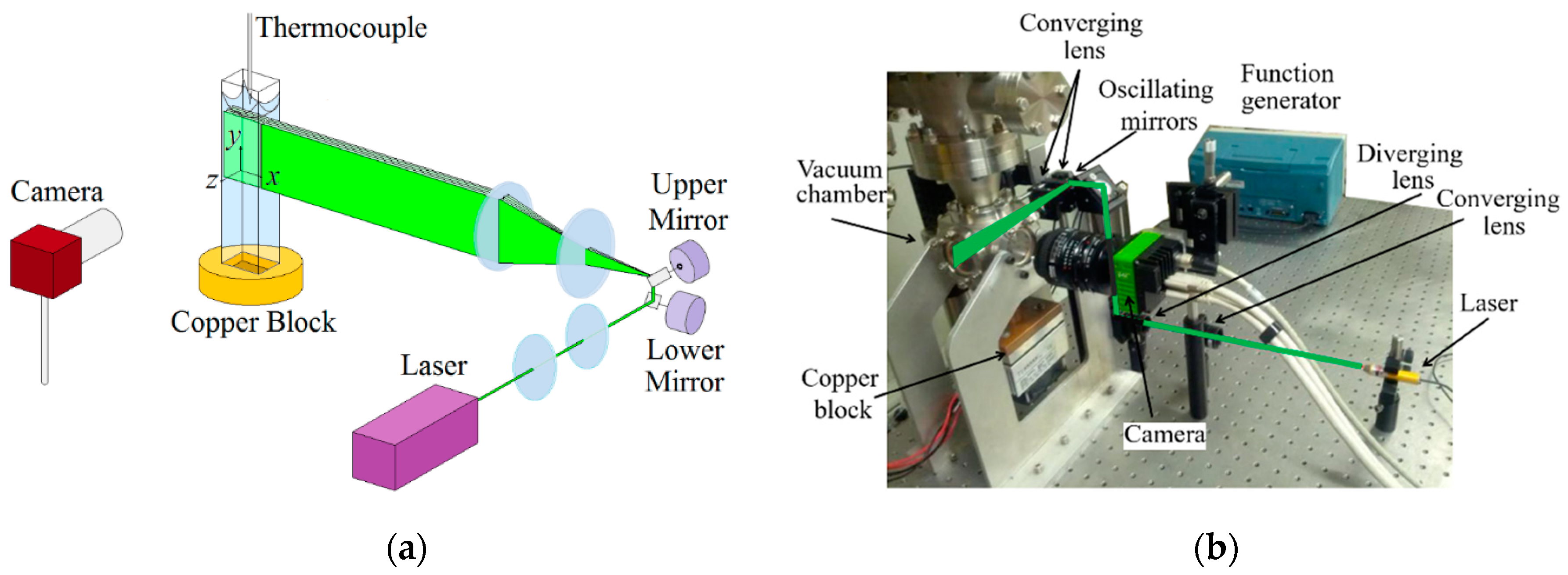
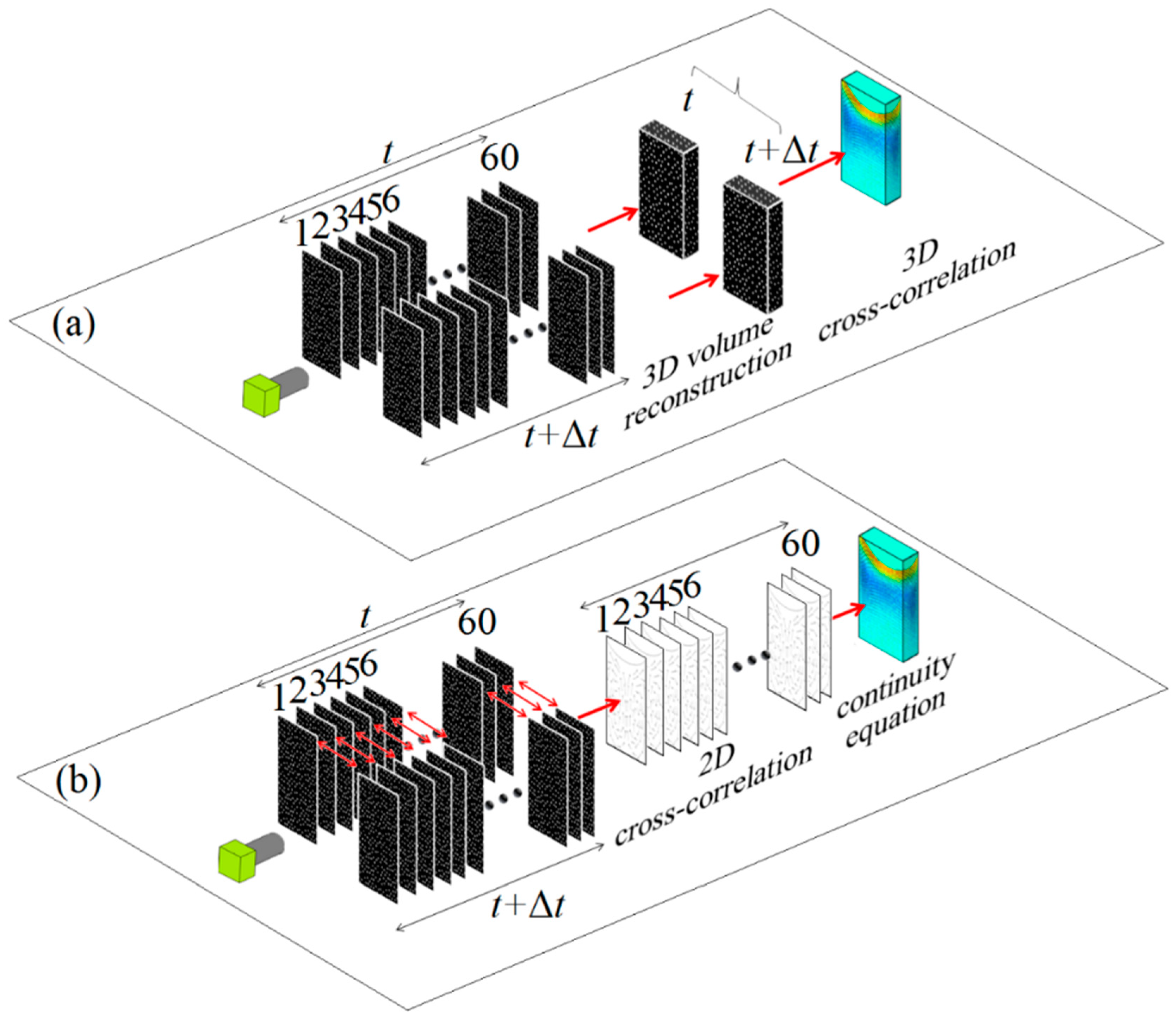
2.2. Scanning PIV System

Scanning PIV requires that a laser sheet scans the volume while a camera captures images of the illuminated planes. An illumination beam was generated by a continuous wave Nd:YAG laser (LRS-0532-PFW-02000-01, LaserGlow Technologies, Toronto, ON, Canada) which emitted green light at 532 nm and delivered an output maximum power of 2 W. To make the 3 mm laser beam narrower, a converging lens with a focal length of 11.1 cm followed by a diverging lens with a focal length of 6.5 cm were installed in front of the laser. This was done to make sure that the laser beam would not spread outside the galvanometer’s moving mirrors (Cambridge Technologies, 6210H, Lexington, MA, USA). The beam was then converted to a scanning laser sheet by being reflected through two orthogonal mirrors. The orientation of the mirrors was controlled by two waveforms produced by a function generator (AFG 3022B, Tektronix Inc., Beaverton, OR, USA). Two other converging lenses (see Figure 1) both having a focal length of 11.1 cm were placed between the mirrors and the cuvette to further narrow the illumination sheet to a thickness of ~150 μm.

As shown in Figure 2a, the function generator created three output voltages to control camera timing while the laser was scanned throughout the volume of interest. The waveform produced by channel 1 (Ch 1) of the function generator consisted of 60 successive rising step functions which was repeated once per second. This waveform controlled the orientation of the lower mirror and moved the laser beam in the depth (z direction). One scan through the depth of the volume was performed for every cycle of this waveform. The signal produced by channel 2 (Ch 2) consisted of many triangle functions which occurred at a high frequency (1250 Hz). This waveform controlled the position of the upper mirror and moved the reflected beam coming from the lower mirror up and down quickly, forming the light sheet. Each triangle in this waveform corresponds to two complete sweeps of the laser beam in the vertical direction (y). This leads to illuminating the in-plane particles during the period that the camera’s shutter is open, making them visible to the camera. A CCD camera (SP-5000M, JAI Inc., San Jose, CA, USA) which had a resolution of 2560 × 2048 pixels recorded the images at up to 134 frames per second. A typical raw image of particles is shown in Figure 2b. The camera was triggered by the transistor–transistor logic (TTL) signal from channel 3 (Ch 3) which was synchronized to Ch 1 and captured 60 images during each scan through the depth of the volume. A small delay of 1.00 ms between the TTL signals of Ch 3 and the step signals of Ch 1 was applied to ensure that the imaging started after the laser sheet had been brought to a complete stop at each depth. A 60 mm single lens reflex (SLR) lens was attached to the camera using three lens extension tubes to focus the particles with a higher magnification. The extended lens delivered a field of view (FOV) of 10.1 mm × 8.1 mm, which is slightly wider than the cuvette’s width (10 mm) and covers 18% of the cuvette’s height. It also provided a depth of field (DOF) of approximately 2 mm, which is half of the cuvette’s depth. A 530 nm high pass filter was placed in front of the camera’s lens to allow only the fluorescent emission to pass and be captured by the camera. The start of image acquisition was controlled by custom software (LabWindows CVI, National Instrument, Austin, TX, USA). The volume was scanned by 60 parallel and overlapping laser sheets at a volume scan rate of 1 Hz. A series of magnified images cropped from 6 consecutive images is shown in Figure 2c. With a total scan depth of 2 mm and sheet thickness of ~0.15 mm, an overlap of 80% is obtained between neighboring slices, which is higher than the minimum of 75% that is required to achieve a good resolution in depth [42]. Finally, the raw images were stored in a computer for later processing.

2.3. Data Processing

An important issue with taking images at various depths with a single camera while the particles remain in focus is the change in magnification of the images. In our experiments, calibration of the furthest and the closest images from/to the camera showed that the calibration factor varied between 3.92 × 10⁻³ mm/pixel and 3.95 × 10⁻³ mm/pixel. This indicates that the maximum change in magnification of the collected images while moving through the depth is 0.7%. Herein, this small change is neglected, and depth-dependent scaling of the images was not performed.

Two different techniques for calculating the three components of velocity are provided. In the first method, as shown in Figure 3a, each set of 60 images that were collected during an individual scan of the volume were stacked together and a 3D volume which includes the 3D positions of the particles in the scanned volume was produced. Using commercial software (DaVis 8.2, LaVision GmbH, Göttingen, Germany), the reconstructed 3D volumes of particle images were cross-correlated and the average displacement of the particle ensembles over a set of voxels in the volume was determined. By knowing the time between each scan, the velocity components were calculated. The cross-correlation was conducted in three steps with different correlation window sizes of 24 × 24 × 24, 20 × 20 × 20 and 16 × 16 × 16 voxels with a 75% overlap which resulted in a spatial resolution of 15.5 µm for the in-plane velocities and ~133 µm for the out-of-plane velocity.

In the second method outlined in Figure 3b, conventional 2D planar PIV is combined with the continuity equation to obtain the out-of-plane component of the velocity. Reconstruction of a 3D velocity field from planar PIV data combined with the continuity equation has been utilized in the past [43,44,45]. In this method, the available 2D images of one scan were cross-correlated with the corresponding images in the next scan which was performed 1 sec later. Using a standard two-component PIV algorithm (DaVis 8.2, LaVision GmbH, Göttingen, Germany), the in-plane components of velocity in 60 planes within the volume were measured. Assuming the suspension is an incompressible fluid, the gradient of the out-of-plane component of velocity may be determined by:

$$\frac{\partial w}{\partial z}=-\left(\frac{\partial u}{\partial x}+\frac{\partial v}{\partial y}\right),$$

(1)

where u, v and w represent the three components of the velocity in x, y and z directions, respectively. The velocity gradients on the right-hand-side of Equation (1) may be approximated using a finite difference scheme. Bown et al. [45] used a second order finite difference in their calculations. However, it has been shown [46] that for the specific experimental study discussed here, the first and second order finite difference schemes did not change the calculated ∂w/∂z. In this work, the derivatives are obtained from a first order finite difference. The coefficients of forward, central and backward approximations are provided by Fornberg [47].

The out-of-plane velocity component, w, may then be approximated using a Taylor series expansion about each individual grid point as:

$$w_{k+1}=w_k+{\left(\frac{\partial w}{\partial z}\right)}_{k+1}\left(\Delta z\right)+O\left(2\right)k=1,2,3,\dots ,59.$$

(2)

The index k refers to the plane number in the out-of-plane, z direction. In the above equation, only the first order derivative is considered, and the higher order terms are truncated. To calculate w in each plane from Equation (2), the first derivative at each plane as well as the boundary value of w (i.e., w₁) should be known. The required derivatives are calculated using Equation (1) and the boundary values of w were obtained from a linear extrapolation toward the solid wall as:

$$w_1=w_{wall}+{\left(\frac{\partial w}{\partial z}\right)}_1{\left(\Delta z\right)}_0,$$

(3)

where ${\left(\Delta z\right)}_0$ is the distance from the center of the first plane to the solid wall and ${\left(\frac{\partial w}{\partial z}\right)}_1$ is the derivative in the first plane. The velocity at the wall is taken to be zero (w_wall = 0) based on the assumption of a no-slip boundary condition at a solid wall.

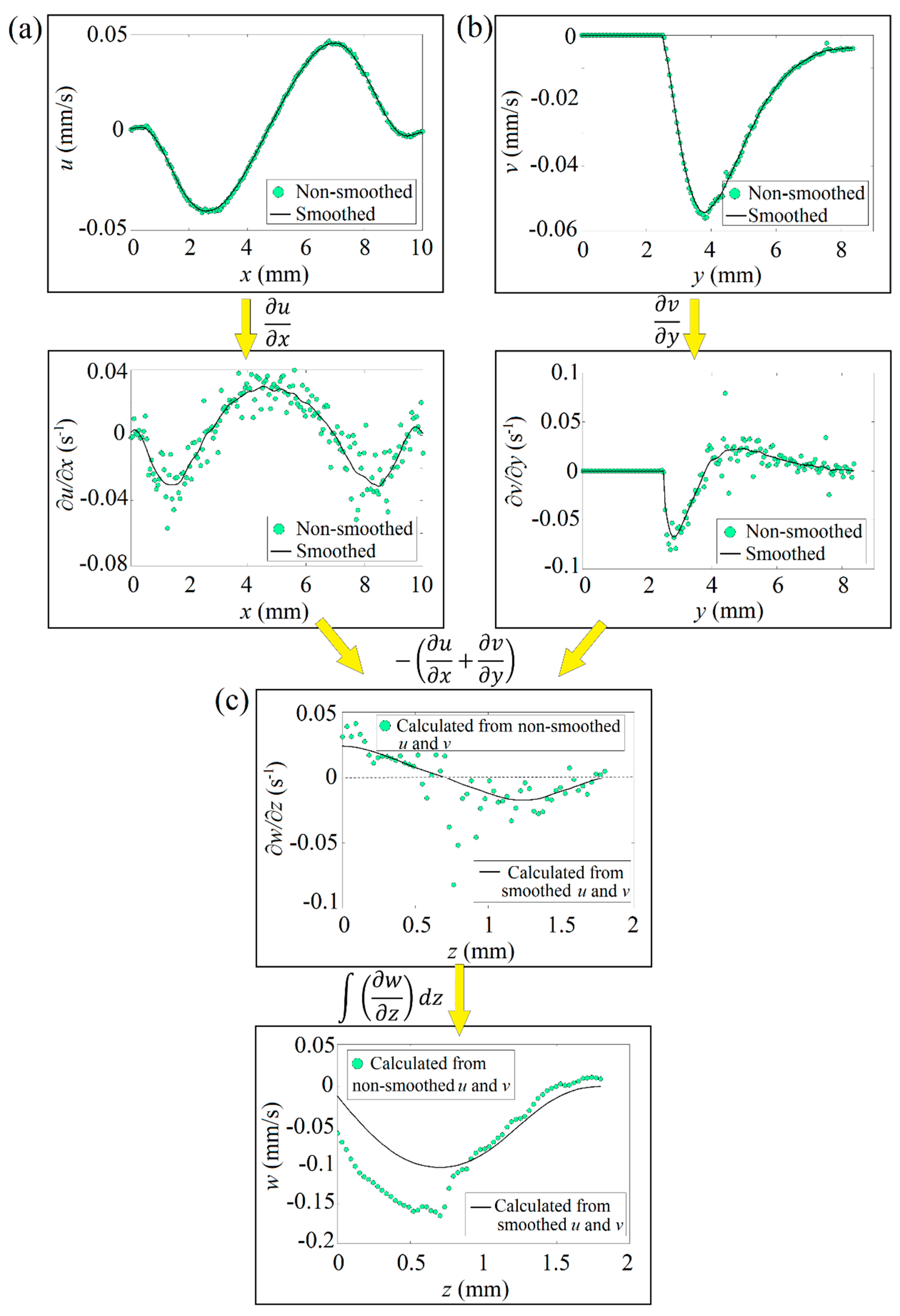
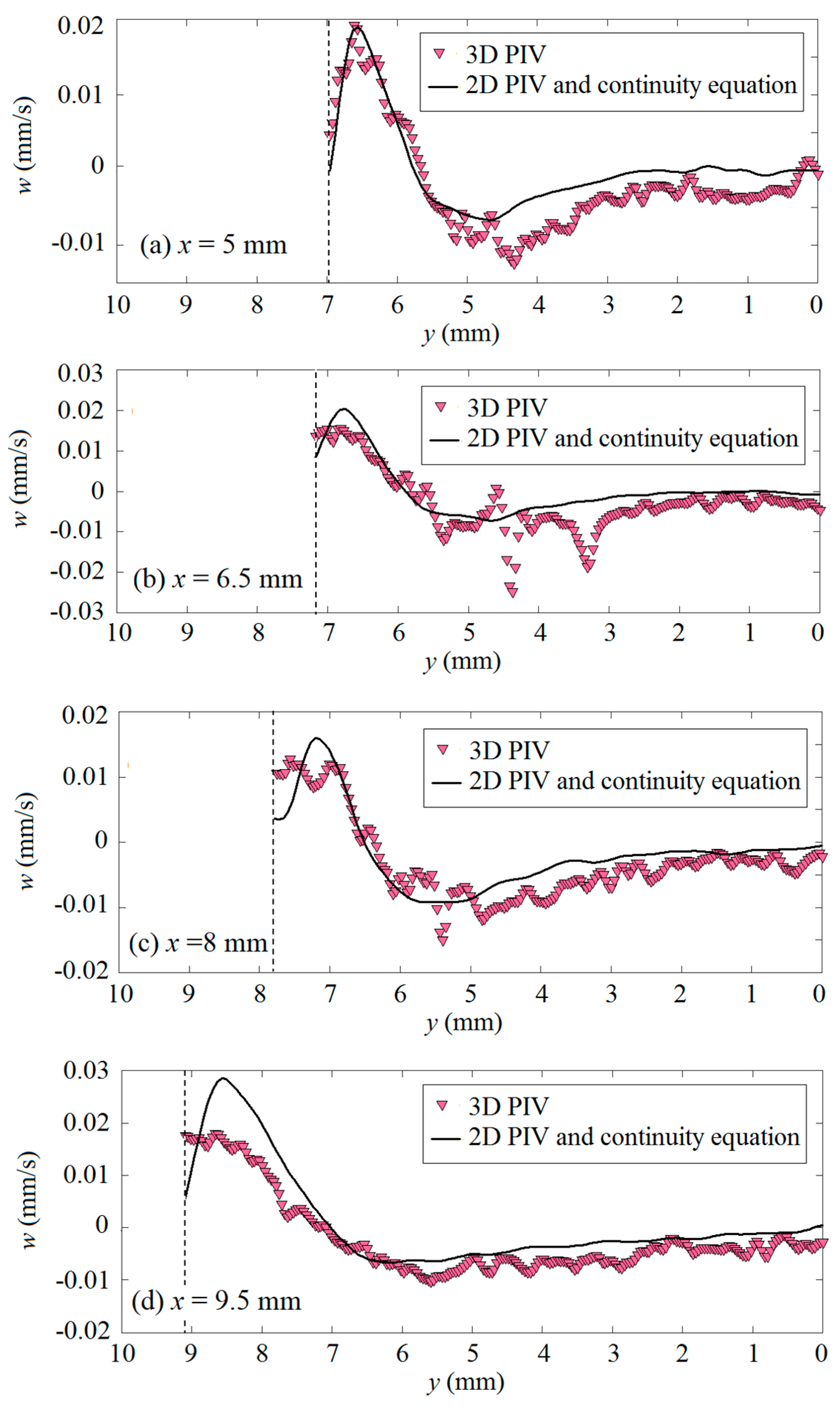
2.4. Determination of Out-Of-Plane Components from Planar PIV and the Continuity Equation

Following the procedures described in the previous sections, the 3D velocity field, including all three velocity components (u, v, w), was obtained. In order to calculate the third component of velocity (w) from the continuity equation, the gradients of the first and the second components (i.e., $\frac{\partial u}{\partial x}$ and $\frac{\partial v}{\partial y}$) needed to be determined. This, in turn, needs the values of u and v in all 60 planes. To accomplish this, the corresponding images from two subsequent volume scans were cross-correlated using a 2D PIV algorithm (DaVis 8.2, LaVision GmbH, Göttingen, Germany) and the u and v components of the velocity were calculated. Cross-correlation was performed in three passes and the final size of the interrogation window used in the PIV process is 16 × 16 (pixel)² which gives a spatial resolution of 15.5 μm in the x and y-directions. The distance between the center of the two overlapping slices is ~ 30 μm which defines the resolution in the z-direction.

To obtain a smooth gradient of w in the z-direction from the continuity equation, the variations of u in the x-direction and v in the y-direction should be smoothed. This is performed by using a 2D smoothing function in commercial code (MATLAB, The Mathworks Inc., Natick, MA, USA). This step was crucial since the gradients are highly sensitive to noise in the velocity field. Figure 4 shows the smoothed vs. the noisy components of the velocity. As can be seen in Figure 4a,b, while the smoothing does not have a significant effect on the velocity components u and v, it strongly influences the gradients $\frac{\partial u}{\partial x}$ and $\frac{\partial v}{\partial y}$. This results in obtaining a more consistent gradient $\frac{\partial w}{\partial z}$ in the depth and subsequently a less noisy w from Equation (2). Figure 4c shows how scattered the calculated w would be if smoothing was not performed on u and v. Note that the calculation scheme starts at the location of known velocity, at the wall where w = 0 at z = 2 mm in Figure 4c and marches into the flow. It is shown in Figure 4c that both values of w start to decrease moving from the front wall on the right side of the image at z = 2 mm to z = 0.7 mm. This is because the gradients in this region are negative. In the regions close to z = 0.7 mm, the negative gradients of the non-smoothed data become large, leading the velocity w to drop suddenly (scattered data). The smoothed gradients, however, vary smoothly and the corresponding values of w do not fall rapidly (solid line). From z = 0.7 mm to the center of the cuvette (z = 0), w starts to increase due to the positive values of the gradients. Note that both scattered and smoothed w show the same trend in this region (both increase with almost the same rate). However, the non-smoothed w cannot approach the smooth solid line since they have already reached to a relatively large negative value at z = 0.7 mm. It can be concluded that the existence of a few outliers in the velocity gradients (which is not far from expectations) while applying the equation of continuity to data obtained from planar PIV can drastically change the calculated velocity component in the third direction.

3. Results and Discussion

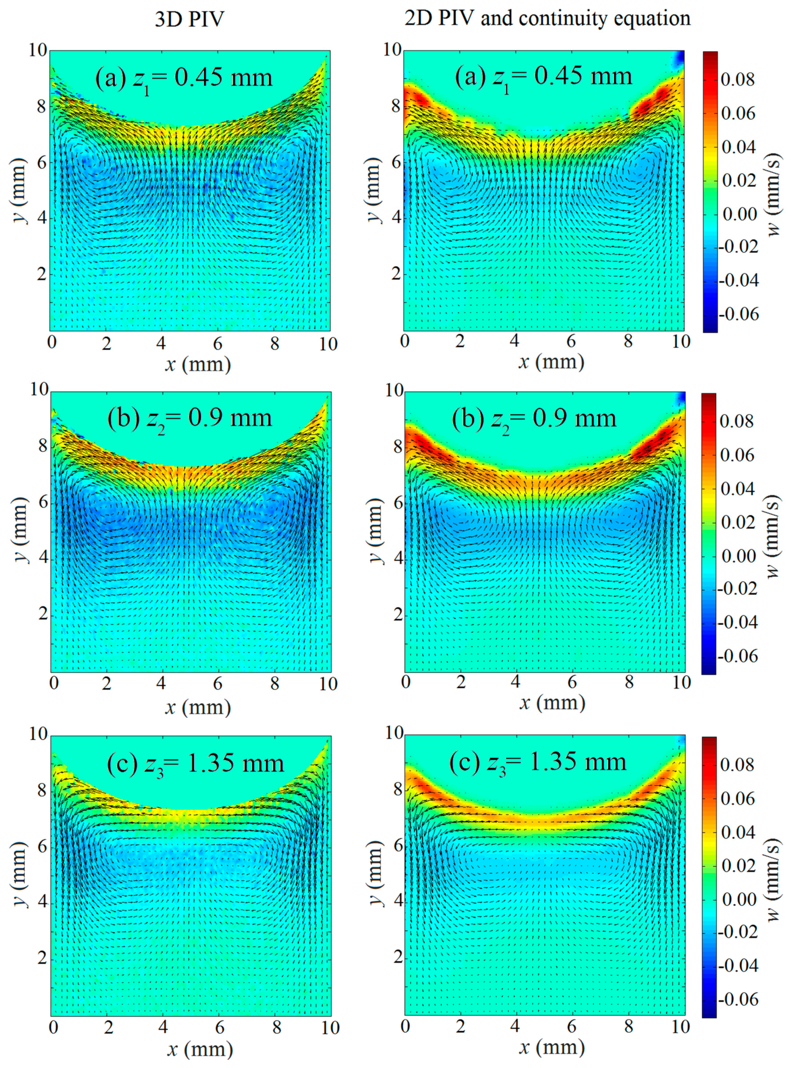
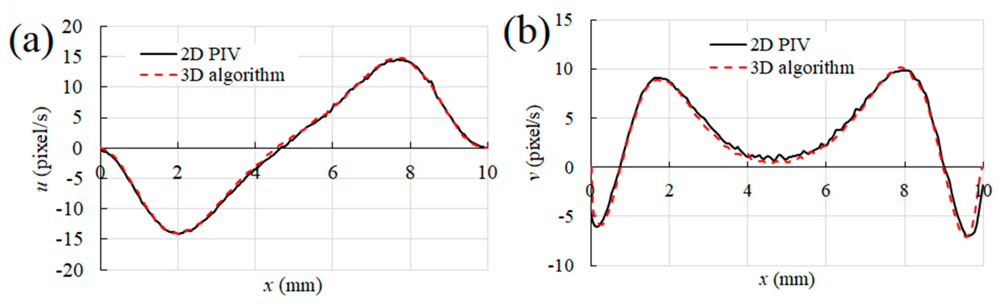
3.1. Comparison of the Generated 3D Velocity Fields

A comparison of the velocity profile obtained from the two different data processing methods is provided in Figure 5. The left three data images show the velocity fields at three arbitrary z-locations obtained from the 3D-PIV algorithm. The right data images show the velocity fields at the same locations obtained from the planar PIV/continuity equation method. The semi-elliptical regions above the yellow colors indicate the regions that were masked out and were not included in the data processing due to the high reflection of light emitted from accumulated particles at the interface. The obtained velocities may be assumed to be the instantaneous velocities since the scan rate of the light sheet through the volume was much higher than the maximum velocity in the liquid (2 mm/s compared to 0.1 mm/s). Both methods revealed the existence of two counter-rotating vortices in the bulk liquid on cross sections parallel to the x-y plane. The centers of the vortices are furthest from each other in the first plane, which is located almost at the center of the cuvette and merge gradually moving toward the last plane, which is close to the cuvette wall. The background color shows the magnitude and direction of the out-of-plane component of the velocity, w. The cyan color indicates the regions where w is close to zero. The yellow and red colors close to the interface represent the regions where the liquid is moving outward while the blue color shows the areas where the liquid is moving in the opposite direction. This implies that the liquid is also rotating in the out-of-plane direction, which cannot be seen in these images.

As can be seen from the velocity vectors in Figure 5 and from the plots in Figure 6, the in-plane velocity components obtained from both methods are in good agreement. However, by looking at Figure 5, one can see that at the interface, especially at the corners where the interface and the walls meet at x = 0 mm and x = 10 mm, the magnitude of w obtained from the continuity equation is noticeably higher than that obtained from the 3D algorithm. This can be seen more clearly in Figure 7 which compares line profiles in the y-direction at a z = 0.45 mm plane from the center for different x-positions. As shown in Figure 7a for x = 5 mm, on the centerline of the cuvette, the calculated values of w from the continuity equation show good agreement with the 3D algorithm. However, the values of w near the interface for side regions close to the wall (Figure 7d) are higher from the continuity equation than from the 3D algorithm, which can be seen in the red regions in Figure 5. This suggests that using the continuity equation to obtain the out-of-plane component of velocity from the smoothed in-plane components may not give reliable results near the boundary regions as the values of w do not meet the zero velocity (no-slip) condition at the solid walls (see the top corner regions in the right-hand-side images of Figure 5). This could be due to the fact that the smoothing has its strongest effects on the boundary data and changes the boundary gradients significantly. Another reason may be that the boundary values of w (w₁ in Equation (3)) are not approximated properly due to the higher sensitivity of the boundary gradients ${\left(\frac{\partial w}{\partial z}\right)}_1$ to the experimental data near the walls and the interface. Although the 3D algorithm gives more reliable data near the boundaries compared to the 2D algorithm/continuity equation, the results of the latter will be demonstrated in the rest of this paper as it gives a smoother velocity field.

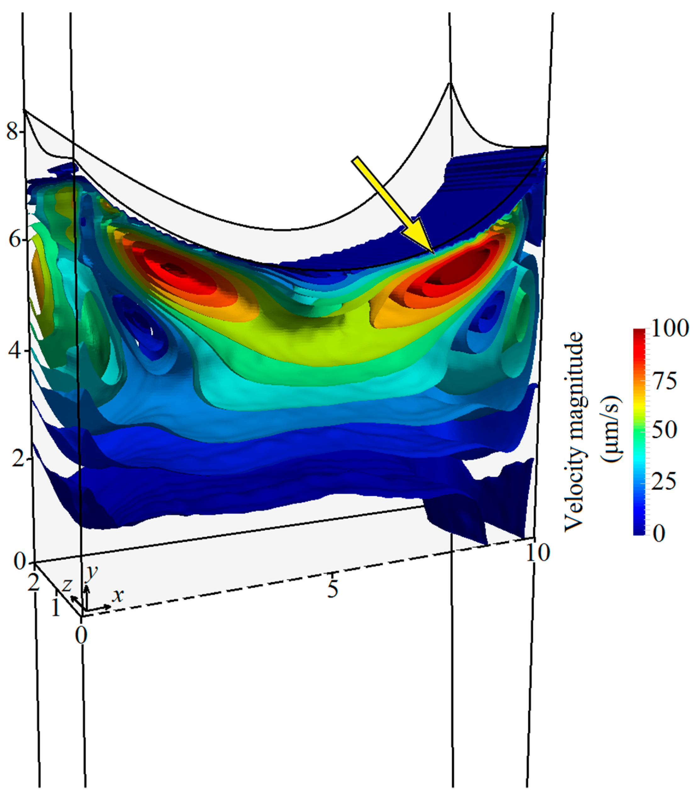
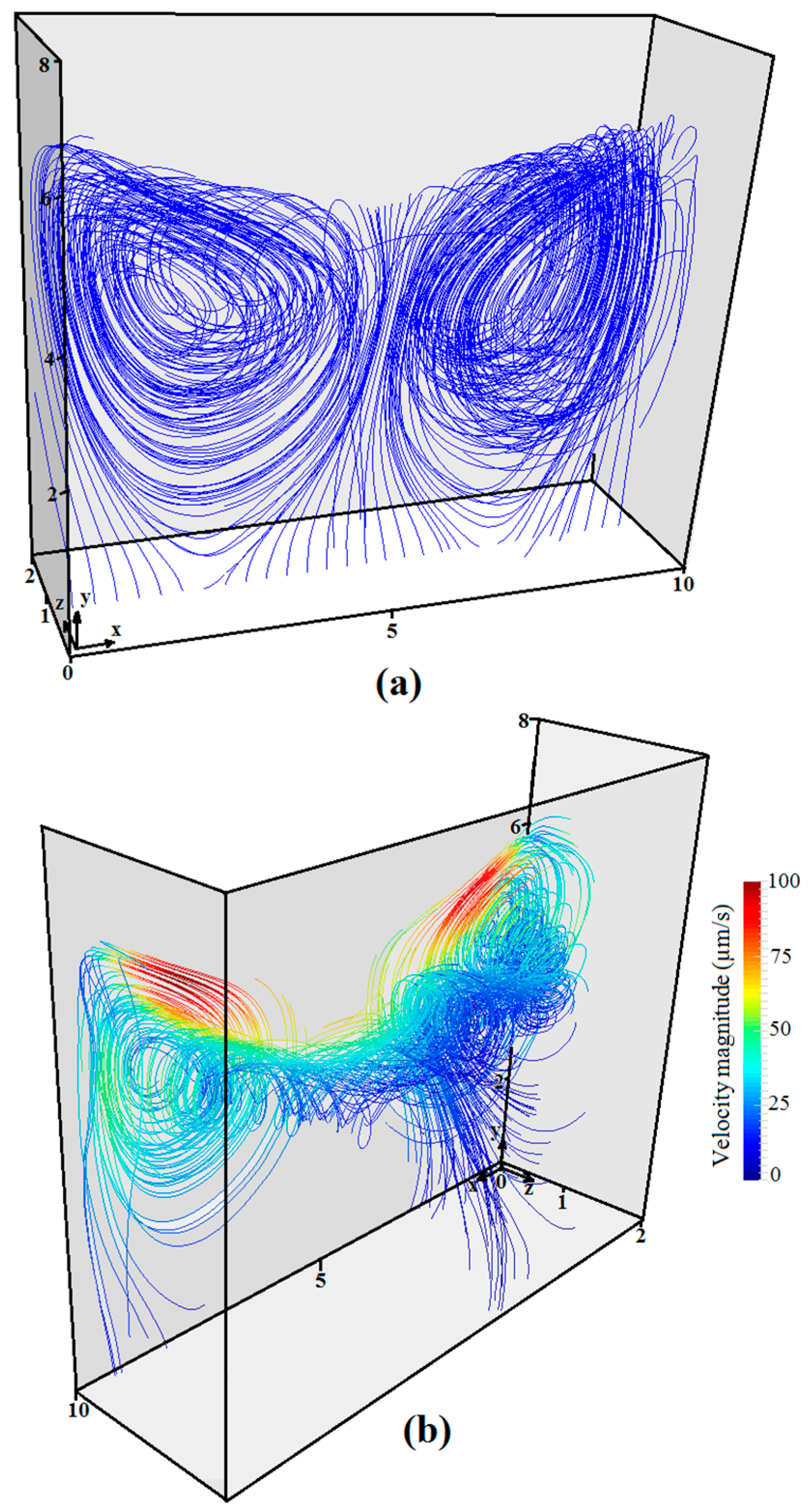
3.2. The 3D Velocity Field of an Evaporating Liquid

Figure 8 demonstrates the 3D velocity arrows in the liquid during the evaporation process obtained from planar PIV combined with the continuity equation. Only every 152nd arrow from 1,720,500 available data points are illustrated here to avoid cluttering the image. The color and the size of the arrows both indicate the local velocity magnitude. The front face in this figure is at the center plane and the back face is located at the back cuvette wall. A small region below the interface containing no velocity arrows can be seen in Figure 8. This region was masked during the image processing and was not studied due to the high reflection of light emitted from accumulated particles at the interface. The measured vector field shows that the flow is quite symmetric. A large toroidal vortex ring can be seen below the evaporating meniscus that occupies the whole cuvette width. This torus shaped motion of the liquid is deformed in the wider direction of the cuvette as a result of the rectangular cross section of the cuvette. Note that only half of this vortex is captured in our PIV experiments due to the limitation in the depth of focus of the lenses. It was shown by numerical simulation that the induced vortex observed here is related to the gravitational forces rather than being driven by the surface tension gradient effects [22].

As Figure 8 shows, in the middle region near the centerline, the liquid moves upward and interacts with the interface, which leads to a sudden decrease in the liquid velocity. This can be noticed from observation of a low-velocity blue region on top of a high-velocity yellow region near the interface at Point A. As the flow reaches the interface, it moves toward the contact lines where the three phases meet (lines BD, DE and EC). This may be due to the higher evaporation rate near the contact lines, similar to the observation for a droplet on a substrate [48]. This observation indicates that the liquid near the interface accelerates on its way toward the contact lines, which is shown by the red arrows in the figure.

It should be noted that in Figure 8 the maximum velocity of ~93 µm/s is attained at a location lower than the interface rather than at the interface. This is not clearly visible in Figure 8 as many of the arrows are eliminated. However, it is clearly shown in Figure 9 which presents 3D velocity magnitude surfaces within the volume. Note the existence of the red layers below the green and blue layers below the interface. This phenomenon has also been observed in two dimensions by Song and Nobes [29] who performed planar PIV on the center plane of an evaporating water in the same cuvette used in this study and also by Li and Yoda [49] in the presence of buoyancy driven convection in a rectangular cavity and in a cylindrical tube in which 2D PIV was performed at the center of the tube during evaporation of water at low pressures [41]. However, the maximum velocity was detected to be exactly at the interface in the evaporation of methanol inside various size microtubes [33].

More details about the flow pattern in three dimensions can be provided by visualizing a number of selected streamlines in the volume. Figure 10 shows the streamlines obtained from the velocity distribution in half of the depth of the cuvette. The figure depicts that in the central region far from the interface, the streamlines are mostly parallel to the vertical axis. However, they become curvilinear as they approach the liquid–vapor interface producing a swirling flow below the interface. The blue torus shaped region below the interface, which starts from the center plane, approaches the front wall and ends on the center plane again roughly showing the location of the vortex core line. This line is closest to the liquid–vapor interface in the central regions and diverges from it moving toward the side regions. Detecting the exact location of the vortex core line is discussed by Jiang et al. [50], which is beyond the scope of this paper.

For the flow of an incompressible liquid, the regions where the streamlines come closer together indicate that the liquid is accelerating based on the conservation of mass, $\dot{m}=\rho VA$, where $\dot{m}$ (kg·s⁻¹) is the local mass flow rate, $\rho$ (kg·m⁻³) is the liquid density, $V$ (m·s⁻¹) is the velocity magnitude and $A$ (m²) is the cross section area of the flow. This is difficult to capture in the 3D representation provided here without looking at the colors. Two dimensional plots of the streamlines in different orthogonal planes are given in Figure 11. The background color shows the velocity magnitude. The streamlines show that the flow is almost symmetric. Cross-sections of the vortex below the interface are revealed in Figure 11a,c but not in Figure 11b since it is located above the vortex core line. It should be mentioned that the 2D streamlines are calculated from the planar components of the velocity on each plane and are not the projection of the 3D streamlines on these planes. However, all three components are taken into account while calculating the velocity magnitude shown in the figure.

4. Conclusions

The liquid flow generated below an evaporating meniscus while experiencing evaporation in a reduced pressure environment was studied and quantified using scanning PIV. The developed technique utilized a laser beam reflected by automated moving mirrors to illuminate the particles and a single camera to capture the images at different depths. Only half of the depth of the cuvette could be studied due to the limitation in the depth of focus of the combined camera lens. A small region below the interface could not be studied because of the interference of the scattered light of accumulated particles.

Two different methods of processing the image into velocity fields were used—one based on the reconstruction of the 3D positions of the particles and the other based on the concept of continuity of an incompressible liquid. Velocity components were calculated in the flow with resolutions as fine as 15 µm on the vertical planes and 30 µm in the depth. It was shown that the out-of-plane velocity (w) calculated from the continuity equation after smoothing the in-plane components (u and v) was in a good agreement with the data obtained from the 3D algorithm. However, the two methods did not show good agreement in the boundary regions near the meniscus corners as smoothing of data affected the velocity values at the boundaries. Further modification to the smoothing algorithm is required to resolve the miscalculation of the boundary velocities.

The 3D reconstruction of the flow revealed a symmetric torus shaped vortex below the meniscus of the evaporating liquid. It was found that the maximum velocities in the flow occurred close to but not exactly at the liquid–vapor interface as would be expected from a surface tension driven flow. The results presented in this paper provide a more detailed description of the flow compared to the previous 2D measurements in evaporating liquids and may be useful to help better understand the phenomena involved in this complicated process as they were in References [22,23,41]. Also, they promise the feasibility of using the continuity equation combined with planar PIV/PTV to be a powerful tool for 3D velocity measurements in applications where current techniques are difficult to be utilized or where a high resolution of the out-of-plane velocity is required to capture the small scales of the flow field. Earlier versions of portions of this work appeared in References [46,51,52].

References

1. Pan, X.; Jin, W.; Liu, Y.; Ai, F. Effect of surface tension-driven flow on BaB2O4 crystal growth from high temperature melt-solution. Cryst. Res. Technol. 2008, 43, 152–156. [Google Scholar] [CrossRef]
2. Sutter, T.; Kim, N.; Kyu, T.; Golovaty, D. Crystal nucleation and motion in an undercooled binary solution. Curr. Opin. Chem. Eng. 2015, 7, 1–5. [Google Scholar] [CrossRef]
3. Savino, R.; di Francescantonio, N.; Fortezza, R.; Abe, Y. Heat pipes with binary mixtures and inverse Marangoni effects for microgravity applications. Acta Astronaut. 2007, 61, 16–26. [Google Scholar] [CrossRef]
4. Di Francescantonio, N.; Savino, R.; Abe, Y. New alcohol solutions for heat pipes: Marangoni effect and heat transfer enhancement. Int. J. Heat Mass Transf. 2008, 51, 6199–6207. [Google Scholar] [CrossRef]
5. Savino, R.; Paterna, D. Marangoni effect and heat pipe dry-out. Phys. Fluids 2006, 18, 2–6. [Google Scholar] [CrossRef]
6. Bhardwaj, R.; Fang, X.; Somasundaran, P.; Attinger, D. Self-assembly of colloidal particles from evaporating droplets: Role of DLVO interactions and proposition of a phase d iagram. Langmuir 2010, 26, 7833–7842. [Google Scholar] [CrossRef] [Green Version]
7. Cai, Y.; Zhang, N.B. Marangoni flow-induced self-assembly of hexagonal and stripelike nanoparticle patterns. J. Am. Chem. Soc. 2008, 130, 6076–6077. [Google Scholar] [CrossRef]
8. Lu, S.; Fujii, H.; Nogi, K. Marangoni convection and weld shape variations in Ar–O2 and Ar–CO2 shielded GTA welding. Mater. Sci. Eng. A 2004, 380, 290–297. [Google Scholar] [CrossRef]
9. Aucott, L.; Dong, H.; Mirihanage, W. Revealing internal flow behaviour in arc welding and additive manufacturing of metals. Nat. Commun. 2018, 9, 5414. [Google Scholar] [CrossRef] [Green Version]
10. Ganzevles, F.L.A.; Van Der Geld, C.W.M. Marangoni convection in binary drops in air cooled from below. Int. J. Heat Mass Transf. 1998, 41, 1293–1301. [Google Scholar] [CrossRef]
11. Trantum, J.R.; Baglia, M.L.; Eagleton, Z.E.; Mernaugh, R.L.; Haselton, F.R. Biosensor design based on Marangoni flow in an evaporating drop. Lab Chip 2014, 14, 315–324. [Google Scholar] [CrossRef] [PubMed]
12. Bénard, H. Les tourbillons cellulaires dans une nappe liquide.-Méthodes optiques d’observation et d’enregistrement. Journal de Physique Théorique et Appliquée 1901, 10, 254–266. [Google Scholar]
13. Block, M.J. Surface tension as the cause of Bénard cells and surface deformation in a liquid film. Nature 1956, 178, 650–651. [Google Scholar] [CrossRef]
14. Pearson, J.R.A. On convection cells induced by surface tension. J. Fluid Mech. 1958, 4, 489–500. [Google Scholar] [CrossRef]
15. Namura, K.; Nakajima, K.; Kimura, K.; Suzuki, M. Photothermally controlled Marangoni flow around a micro bubble. Appl. Phys. Lett. 2015, 106, 043101. [Google Scholar] [CrossRef] [Green Version]
16. Chai, A.T.; Zhang, N. Experimental study of MArangoni-Benard convection in a liquid layer induced by evaporation. Exp. Heat Transf. 1998, 11, 187–205. [Google Scholar] [CrossRef]
17. Masoud, H.; Felske, J.D. Analytical solution for inviscid flow inside an evaporating sessile drop. Phys. Rev. E 2009, 79, 016301. [Google Scholar] [CrossRef] [Green Version]
18. Zheng, L.; Zhang, X.; Gao, Y. Analytical solution for Marangoni convection over a liquid–vapor surface due to an imposed temperature gradient. Math. Comput. Model. 2008, 48, 1787–1795. [Google Scholar] [CrossRef]
19. Tam, D.; Von Arnim, V.; McKinley, G.H.; Hosoi, A.E. Marangoni convection in droplets on superhydrophobic surfaces. J. Fluid Mech. 2009, 624, 101–123. [Google Scholar] [CrossRef] [Green Version]
20. Schmitt, M.; Stark, H. Marangoni flow at droplet interfaces: Three-dimensional solution and applications. Phys. Fluids 2016, 28, 012106. [Google Scholar] [CrossRef] [Green Version]
21. Hu, H.; Larson, R.G. Evaporation of asessile droplet on a substrate. J. Phys. Chem. B 2002, 106, 1334–1344. [Google Scholar] [CrossRef]
22. Kazemi, M.A.; Nobes, D.S.; Elliott, J.A.W. Investigation of the phenomena occurring near the liquid–vapor interface during evaporation of water at low pressures. Phys. Rev. Fluids 2018, 3, 124001. [Google Scholar] [CrossRef]
23. Kazemi, M.A.; Elliott, J.A.W.; Nobes, D.S. The influence of container geometry and thermal conductivity on evaporation of water at low pressures. Sci. Rep. 2018, 8, 15121. [Google Scholar] [CrossRef] [PubMed] [Green Version]
24. Duan, F.; Ward, C.A. Surface-thermal capacity of D2O from measurements made during steady-state evaporation. Phys. Rev. E 2005, 72, 056304. [Google Scholar] [CrossRef] [PubMed]
25. Ward, C.A.; Duan, F. Turbulent transition of thermocapillary flow induced by water evaporation. Phys. Rev. E 2004, 69, 056308. [Google Scholar] [CrossRef] [PubMed]
26. Ghasemi, H.; Ward, C.A. Energy transport by thermocapillary convection during sessile-water-droplet evaporation. Phys. Rev. Lett. 2010, 105, 136102. [Google Scholar] [CrossRef] [PubMed]
27. Thompson, I.; Duan, F.; Ward, C.A. Absence of Marangoni convection at Marangoni numbers above 27,000 during water evaporation. Phys. Rev. E 2009, 80, 056308. [Google Scholar] [CrossRef]
28. Mancini, H.; Maza, D. Pattern formation without heating in an evaporative convection experiment. Eur. Lett. 2004, 66, 812–818. [Google Scholar] [CrossRef]
29. Song, X.; Nobes, D.S. Experimental investigation of evaporation-induced convection in water using laser based measurement techniques. Exp. Therm. Fluid Sci. 2011, 35, 910–919. [Google Scholar] [CrossRef]
30. Babaie, A.; Madadkhani, S.; Stoeber, B. Evaporation-driven low Reynolds number vortices in a cavity. Phys. Fluids 2014, 26, 033102. [Google Scholar] [CrossRef]
31. Thokchom, A.K.; Gupta, A.; Jaijus, P.J.; Singh, A. Analysis of fluid flow and particle transport in evaporating droplets exposed to infrared heating. Int. J. Heat Mass Transf. 2014, 68, 67–77. [Google Scholar] [CrossRef]
32. Buffone, C.; Sefiane, K.; Christy, J.R.E. Experimental investigation of self-induced thermocapillary convection for an evaporating meniscus in capillary tubes using micro–particle image velocimetry. Phys. Fluids 2005, 17, 052104. [Google Scholar] [CrossRef]
33. Dhavaleswarapu, H.K.; Chamarthy, P.; Garimella, S.V.; Murthy, J.Y. Experimental investigation of steady buoyant-thermocapillary convection near an evaporating meniscus. Phys. Fluids 2007, 19, 082103. [Google Scholar] [CrossRef] [Green Version]
34. Minetti, C.; Buffone, C. Three-dimensional Marangoni cell in self-induced evaporating cooling unveiled by digital holographic microscopy. Phys. Rev. E 2014, 89, 1–6. [Google Scholar] [CrossRef]
35. Li, S.; Chen, R.; Zhu, X.; Liao, Q. Numerical investigation of the Marangoni convection during the liquid column evaporation in microchannels caused by IR laser heating. Int. J. Heat Mass Transf. 2016, 101, 970–980. [Google Scholar] [CrossRef]
36. Pereira, F.; Gharib, M.; Dabiri, D.; Modarress, D. Defocusing digital particle image velocimetry: A 3-component 3-dimensional DPIV measurement technique. Application to bubbly flows. Exp. Fluids 2000, 29, S078–S084. [Google Scholar] [CrossRef]
37. Elsinga, G.E.; Scarano, F.; Wieneke, B.; Van Oudheusden, B.W. Tomographic particle image velocimetry. Exp. Fluids 2006, 41, 933–947. [Google Scholar] [CrossRef]
38. Sheng, J.; Malkiel, E.; Katz, J. Using digital holographic microscopy for simultaneous measurements of 3D near wall velocity and wall shear stress in a turbulent boundary layer. Exp. Fluids 2008, 45, 1023–1035. [Google Scholar] [CrossRef]
39. Burgmann, S.; Schröder, W. Investigation of the vortex induced unsteadiness of a separation bubble via time-resolved and scanning PIV measurements. Exp. Fluids 2008, 45, 675–691. [Google Scholar] [CrossRef]
40. Gao, Q.; Wang, H.; Shen, G. Review on development of volumetric particle image velocimetry. Chin. Sci. Bull. 2013, 58, 4541–4556. [Google Scholar] [CrossRef]
41. Kazemi, M.A.; Nobes, D.S.; Elliott, J.A.W. Experimental and numerical study of the evaporation of water at low pressures. Langmuir 2017, 33, 4578–4591. [Google Scholar] [CrossRef] [PubMed] [Green Version]
42. Brücker, C.; Hess, D.; Kitzhofer, J. Single-view volumetric PIV via high-resolution scanning, isotropic voxel restructuring and 3D least-squares matching (3D-LSM). Meas. Sci. Technol. 2013, 24, 024001. [Google Scholar] [CrossRef]
43. Kinoshita, H.; Kaneda, S.; Fujii, T.; Oshima, M. Three-dimensional measurement and visualization of internal flow of a moving droplet using confocal micro-PIV. Lab Chip 2007, 7, 338–346. [Google Scholar] [CrossRef] [PubMed]
44. Robinson, O.; Rockwell, D. Construction of three-dimensional images of flow structure via particle tracking techniques. Exp. Fluids 1993, 14, 257–270. [Google Scholar] [CrossRef]
45. Bown, M.R.; MacInnes, J.M.; Allen, R.W.K. Three-component micro-PIV using the continuity equation and a comparison of the performance with that of stereoscopic measurements. Exp. Fluids 2007, 42, 197–205. [Google Scholar] [CrossRef]
46. Kazemi, M.A.; Elliott, J.A.W.; Nobes, D.S. Determination of the three components of velocity in an evaporating liquid from scanning PIV. In Proceedings of the 18th International Symposium on the Application of Laser and Imaging Techniques to Fluid Mechanics, Lisbon, Portugal, 4–7 July 2016. [Google Scholar]
47. Fornberg, B. Generation of finite difference formulas on arbitrarily spaced grids. Math. Comput. 1988, 51, 699–706. [Google Scholar] [CrossRef]
48. Deegan, R.D.; Bakajin, O.; Dupont, T.F.; Huber, G.; Nagel, S.R.; Witten, T.A. Contact line deposits in an evaporating drop. Phys. Rev. E 2000, 62, 756–765. [Google Scholar] [CrossRef] [Green Version]
49. Li, Y.; Yoda, M. Convection driven by a horizontal temperature gradient in a confined aqueous surfactant solution: The effect of noncondensables. Exp. Fluids 2014, 55, 1663. [Google Scholar] [CrossRef]
50. Jiang, M.; Machiraju, R.; Thompson, D. Detection and visualization of vortices. In Visualization Handbook; Elsevier: Amsterdam, The Netherlands, 2005; pp. 295–309. [Google Scholar] [CrossRef]
51. Kazemi, M.A. Experimental and Numerical Study on Evaporation of Water at Low Pressures. PhD Thesis, University of Alberta, Edmonton, AB, Canada, 2017. Available online: https://era.library.ualberta.ca/items/d7d41d86-14b4-4e42-8e2f-95d46ff0749c/view/65ce8735-485f-4554-861f-058951eefd2d/Kazemi_Mohammad-20Amin_201709_PhD.pdf (accessed on 10 October 2017).
52. Kazemi, M.A.; Elliott, J.A.W.; Nobes, D.S. A 3D flow visualization in evaporation of water from a meniscus at low pressures. In Proceedings of the 10th Pacific Symposium on Flow Visualization and Image Processing, Naples, Italy, 15–18 June 2015; Available online: https://www.psfvip10.unina.it/Ebook/web/papers/199_PSFVIP10.pdf (accessed on 30 June 2015).
Figure 1. The experimental configuration: (a) a schematic diagram of the scanning particle image velocimetry (PIV) experiment where the cuvette and optics are magnified for clarity and (b) an image of the real system setup. The laser shown here was only used for optical allignment purposes and is not the actual one used in the experiments.
Optics 01 00005 g001
Figure 2. (a) Timing diagram of control signals to trigger the camera in sync with the moving mirrors. The rising step function (red) propels the light sheet in the depth and the camera that is triggered by the rectangular function (blue) records the images of particles at different depths. (b) A typical image taken at the center of the cuvette. The accumulation of particles at the interface caused the interface to appear shiny. (c) The magnified images cropped from 6 consecutive images as the light sheet travels in depth. Note how the typically shown particles appear and disappear in the images as the light sheet scans the volume.
Optics 01 00005 g002
Figure 3. An illustration of the two different methods of image processing to calculate the three components of velocity: (a) shows a 3D cross-correlation algorithm and (b) shows a 2D algorithm combined with the continuity equation.
Optics 01 00005 g003
Figure 4. The effect of the smoothing of in-plane velocity components, u and v, on the calculated velocity component w from Equation (2). (a) shows the smoothed and non-smoothed u and its gradient at y = 5 mm and z = 0.3 mm. (b) shows the smoothed and non-smoothed v and its gradient at x = 5 mm and z = 0.3 mm (c) shows the calculated gradient of w and calculated w, based on smoothed and non-smoothed u and v at x = 5 mm and y =5 mm.
Optics 01 00005 g004
Figure 5. A comparison of the velocity components obtained from two different methods of processing the images at three planes (a) z1 = 0.45 mm, (b) z2 = 0.9 mm and (c) z3 = 1.35 mm from the center. The arrows show u and v, the background color shows w. The left three plots are obtained from 3D PIV. The three right plots are the results of the 2D processing coupled with the continuity equation.
Optics 01 00005 g005
Figure 6. Comparison between the in-plane velocities (a) u and (b) v obtained from the 2D PIV and 3D algorithms. The velocities were extracted from the centerplane (z = 0) and y = 6.5 mm.
Optics 01 00005 g006
Figure 7. A comparison of the out-of-plane component of velocity w obtained from the 3D algorithm and from the continuity equation at a plane 0.45 mm from the center and (a) x = 5 mm, (b) x = 6.5 mm, (c) x = 8 mm and (d) x = 9.5 mm. x = 5 mm is at the center plane and x = 10 mm shows the cuvette side wall. The dashed lines show the closest regions to the interface.
Optics 01 00005 g007
Figure 8. Three-dimensional velocity vectors below the evaporating meniscus. The arrow size and color scale to the local velocity magnitude.
Optics 01 00005 g008
Figure 9. The contours of constant velocity in the volume. The region indicated by the arrow shows that the maximum velocity occurs below the interface, not at the interface. z = 0 is at the center plane and z = 2 mm is at the cuvette’s wall. See Figure 8 for more information about the geometry.
Optics 01 00005 g009
Figure 10. A representation of some selected streamlines in 3D. The origin of the streamlines in (a) is a horizontal line at z = 1 mm and y = 0 mm. The origin of the streamlines in (b) is a number of points in the plane located at z = 0 mm. The colors in (b) show the local velocity magnitude.
Optics 01 00005 g010
Figure 11. Two-dimensional streamlines on three arbitrary planes parallel to the (a) xy plane (front view), (b) xz plane (top view) and (c) yz plane (side view). The dotted lines show the positions of the planes in the other orthogonal views.
Optics 01 00005 g011