Simultaneous Stereo PIV and MPS³ Wall-Shear Stress Measurements in Turbulent Channel Flow

Abstract

An extended experimental method is presented in which the micro-pillar shear-stress sensor (MPS${}^3$) and high-speed stereo particle-image velocimetry measurements are simultaneously performed in turbulent channel flow to conduct concurrent time-resolved measurements of the two-dimensional wall-shear stress (WSS) distribution and the velocity field in the outer flow. The extended experimental setup, which involves a modified MPS${}^3$ measurement setup and data evaluation compared to the standard method, is presented and used to investigate the footprint of the outer, large-scale motions (LSM) onto the near-wall small-scale motions. The measurements were performed in a fully developed, turbulent channel flow at a friction Reynolds number $R{e}_{\tau }=969$. A separation between large and small scales of the velocity fluctuations and the WSS fluctuations was performed by two-dimensional empirical mode decomposition. A subsequent cross-correlation analysis between the large-scale velocity fluctuations and the large-scale WSS fluctuations shows that the streamwise inclination angle between the LSM in the outer layer and the large-scale footprint imposed onto the near-wall dynamics has a mean value of ${\overline{\Theta }}_x={16.53}^{\circ }$, which is consistent with the literature relying on direct numerical simulations and hot-wire anemometry data. When also considering the spatial shift in the spanwise direction, the mean inclination angle reduces to ${\overline{\Theta }}_{xz}={13.92}^{\circ }$.

1. Introduction

The simultaneous spatial and temporal resolution of the two-dimensional wall-shear stress (WSS) distribution and the outer flow field in experimental measurements is rather challenging. However, to broaden the knowledge of, e.g., the internal structure of turbulent wall-bounded flows, such concurrent measurements are necessary. Previous approaches, e.g., by Mathis et al. [1], Baars et al. [2], used intrusive hot-wire anemometry (HWA) methods to resolve the flow field in the near-wall region and in the outer layer of a turbulent boundary layer (TBL). This technique is one of the basic measurement methods in fluid mechanics due to its accessibility and reasonable compromises, e.g., the drawback of only providing pointwise information [3]. This point measurement requires Taylor’s hypothesis to transform the temporal data into spatial information.

Many alternative techniques to measure the WSS exist and comprehensive reviews are given, e.g., in [4,5,6,7]. The WSS devices can be divided in direct and indirect measurement methods. The most commonly used direct WSS sensors include thin oil-film techniques, shear stress sensitive liquid crystals, and floating element shear stress sensors. When using thin oil films, the major cause of uncertainty is the accurate determination of the oil viscosity and temperature leading to measurement uncertainties of around $5\%$ at optimum conditions [5]. With respect to the current investigation, liquid crystals possess the disadvantage of not providing the required resolution to measure turbulent WSS fluctuations [7]. The use of floating elements involves a trade-off between spatial resolution and the ability of the sensor to measure small forces [7], which is usually unacceptable in terms of accurate WSS fluctuation determination.

Indirect WSS sensors include, among others, thermal WSS sensors, pressure fence sensors, optical methods, and deflection elements. HWA methods, which belong to the group of thermal sensors, have already been discussed earlier. Another thermal WSS sensor is the hot film, which is based on a similar measurement principle as the HWA. It is directly mounted at the surface and, thus, a frequency dependent leakage of heat transfer into the surrounding substrate causes inaccuracies of the dynamic sensor response [7]. An alternative, non-intrusive optical measurement technique is the micro-particle tracking velocimetry ($\mu$-PTV). It determines the WSS based on its relation to the velocity gradient at the wall ${\tau }_w{=-\eta \partial u/\partial y|}_{y=0}$. Although $\mu$-PTV provides highly resolved spatial data, it is currently only able to capture the one-dimensional evolution of the near-wall dynamics and time-resolved investigations are difficult to conduct due to the typically low seeding density in the near-wall region [8]. Research in the field of bionics inspired the development of deflection element based WSS sensors usually consisting of flexible cantilevers or micro-posts. Often, they are only used to quantitatively or qualitatively determine the local flow field, as investigations of, e.g., the trichobothria on the walking legs of spiders [9] or the primary cilia in endothelial cells of the chicken embryonic endocardium [10], showed. Nevertheless, their working principle is very similar to that of the micro-pillar shear-stress sensor (MPS${}^3$). The sensor consists of surface-mounted, flexible, cylindrical structures that bend due to the exerted fluid forces and this deflection can directly be correlated with the WSS. The MPS${}^3$ has already been successfully used in a variety of flow cases, e.g., a TBL with zero-pressure gradient [11] as well as with adverse-pressure gradient [12], pipe flow [13], and duct flow [14]. In contrast to the WSS sensors mentioned above, the MPS${}^3$ comprises all the advantages of low intrusiveness, high sensitivity even to very small WSS fluctuations, two-dimensional and excellent spatial resolution, and the possibility to acquire time-resolved data.

To investigate the structural organization in wall-bounded flows, recent research focuses on the different types of near-wall small-scale modulation by large-scale motions (LSM) of the outer layer using direct numerical simulations (DNS) (e.g., [15,16,17]), and HWA measurements (e.g., [1,18]). Basically, the small-scale motions (SSM) are influenced by three mechanisms, namely superposition, amplitude and frequency modulation, and distortions by sweeps and ejections [15]. The superposition is essentially a streamwise shift imposed onto the universal behavior of the SSM and often referred to as footprinting. It features a time shift between the LSM occurring in the outer layer and their imposed footprint near the wall. In addition, the LSM influence the frequency and amplitude of the SSM. Recent research states that this process is not to be seen as a direct interaction between SSM and LSM but rather introduced by variations in the shear-induced production due to changes in the conditional velocity profile [17]. The extent of the modulation varies with wall distance. Sweeps and ejections are local swerves inside the flow leading to an asymmetric modulation of the near-wall SSM [15].

To properly determine the interaction between LSM and SSM, the flow structures need to be carefully separated from each other. Although several procedures and models are introduced in the literature, no strict criterion for scale separation exists so far [19]. Among others, Liu et al. [20] used Proper Orthogonal Decomposition (POD), which is a generalization of conventional Fourier power spectral analysis, to extract the contribution of each mode to the energy and the Reynolds stresses as a function of scales. The authors applied POD to two-dimensional spatial correlations of particle-image velocimetry (PIV) data and showed that most of the energy and Reynolds stresses is carried by a small number of eigenmodes, which they claimed to represent the LSM. Summing up these highly energetic modes works like a spatial low-pass filter similar to the procedure used, e.g., by Mathis et al. [21]. In their study, which is based on HWA measurements, the authors conducted a frequency based high-pass filtering to obtain the large-scale velocity and WSS components. Since the LSM feature a relatively uniform streamwise velocity magnitude, researchers also investigated these structures by detecting so-called uniform momentum zones [22,23]. Another scale separation strategy is based on two-dimensional Empirical Mode Decomposition (EMD). This algorithm, which was originally proposed by Huang et al. [24], splits amplitude- or frequency-modulated signals into a set of Intrinsic Mode Functions (IMF) based on the local characteristic time or space scales. By comparing the EMD to other separation algorithms and taking into consideration several studies concerning its efficacy and validity, Agostini and Leschziner [15] showed that the EMD is well suited to separate the large from the small scales. Since the energy content of the large scales is comparable to the small-scale energy at high Reynolds numbers, POD will not lead to convincing results. Moreover, no pre-determined functional elements are needed for the EMD like for Fourier or wavelet functions [15].

In this study, an extended approach is introduced, which enables the analysis of the impact of outer layer LSM on near-wall SSM in a direct, temporally and spatially resolved experimental measurement. To the authors’ knowledge, this has not been performed for wall-bounded flows; however, it offers new opportunities in this field of study. Compared to previous experimental investigations, the present setup does not require Taylor’s hypothesis, which is necessary when using HWA methods (e.g., [1,18]), since it is able to resolve the WSS distribution and the outer flow field in the streamwise and spanwise direction. In addition, a spatial resolution in both directions similar to DNS (e.g., [15,25]) is achieved, which allows direct comparisons between experimental and numerical data.

The novel approach combines the MPS${}^3$, which measures the time-resolved, two-dimensional WSS distribution, with simultaneous time-resolved, stereo, high-speed PIV measurements that capture the outer velocity field in TCF. A detailed analysis is conducted concerning any possible interference between both measurement techniques. As a first step, the current investigation focuses on the most fundamental large-scale influence, the footprinting of LSM. Since the results are compared to the conclusions drawn from DNS and HWA measurements, the evaluation methods are based on the tools used in the literature. Hence, a two-dimensional EMD is used to separate the large-scale components of the WSS fluctuations and the velocity fluctuations. For each time step, a cross-correlation between the large-scale distributions reveals the spatial delay of the LSM imposed onto the near-wall dynamics and, thus, the corresponding inclination angle.

This manuscript is organized as follows. First, the MPS${}^3$ and the experimental setup are described in detail. Subsequently, the methods to evaluate the data obtained by MPS${}^3$ and PIV measurements are presented. The results cover the investigation of possible influences of the seeding particles that are necessary to conduct PIV measurements on the MPS${}^3$ as well as the analysis of the large-scale footprints imposed onto the near-wall dynamics. Finally, the results are briefly summarized and an outlook for future work is given.

2. Micro-Pillar Shear-Stress Sensor (MPS${}^3$)

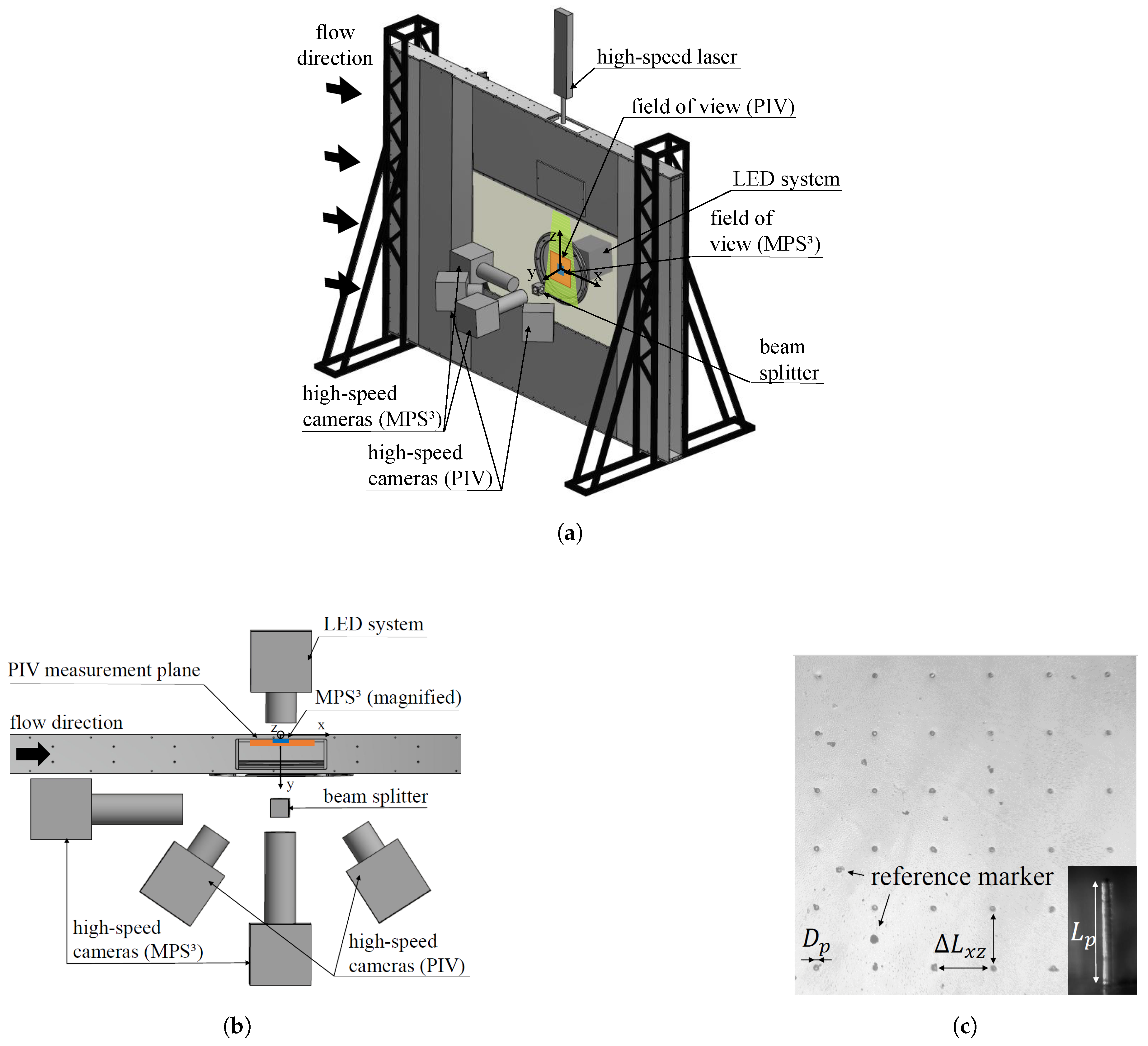
The MPS${}^3$ enables the acquisition of the two-dimensional WSS distribution with excellent spatial and temporal resolution. The sensor consists of flexible, cylindrical structures, so-called micro pillars, made from the polymer polydimethylsiloxane. An image is shown in Figure 1c with a zoom of the sensor. The MPS${}^3$ is flush-mounted onto the measurement surface and the geometry of the micro pillars is adapted to the height of the viscous sublayer ensuring only a local disturbance of the flow field. The micro pillars bend due to the exerted fluid forces and, for small deflections, which are always ensured by adjusting the MPS${}^3$ properties to the specific flow case, the deflections can be described by linear bending theory. For a detailed description of the working principle, please refer to, e.g., the works of Große and Schröder [14] and Große et al. [26].

In previous measurements (e.g., [27]), a continuous laser light sheet was used to illuminate a plane parallel to the measurement surface exposing reflective hollow spheres that were attached to the tips of the micro pillars. This setup requires a careful adjustment of the light sheet, since large micro-pillar deflections can move the micro-pillar tip out of the illuminated plane. In the current investigation, a pulsed high-speed LED system is used in a backlight configuration similar to shadowgraphy [28], which has several advantages. First, the thermal loads imposed onto the MPS${}^3$ are lowered resulting in less variations of the mechanical properties of the sensor during the measurement. Second, especially with respect to the simultaneous PIV measurements, the backlight configuration reduces the complexity of the measurement setup without a loss of accuracy. Since not only the micro-pillar tips but also the whole sensor is illuminated, no out-of-plane movement of the micro-pillar tips can spoil the measurements. In addition, the need to apply reflective spheres to the tips is no longer justified, which, on the one hand, reduces the manufacturing time of the MPS${}^3$ and, on the other hand, leads to a more precise approximation of the micro-pillar behavior, as described by linear bending theory. The latter is especially useful in predicting the MPS${}^3$ behavior with respect to the selection of the sensor properties for different applications. In conclusion, the novel illumination strategy reduces the manufacturing and measurement setup complexity of the MPS${}^3$ while additionally increasing the accuracy of the WSS determination through stabilized mechanical sensor properties and improved micro-pillar detection. The latter is accompanied by a superior detection algorithm, which is explained in the description of the WSS determination.

To obtain the WSS distribution from the MPS${}^3$ measurements, each MPS${}^3$ image at flow condition is compared to a reference image at zero velocity. The resulting micro-pillar tip deflection is converted to the WSS based on a previously performed calibration. Since the MPS${}^3$ setup is highly sensitive due to the large optical magnification, minor movements of the camera, e.g., introduced by wind tunnel vibrations, lead to a shift of the field of view. Hence, this background movement has to be eliminated prior to the evaluation of the micro-pillar deflections. This is achieved by performing cross-correlation between the reference image at zero flow and the run image at flow condition at various reference markers distributed across the whole MPS${}^3$. A sub-pixel accurate determination of the displacement of each individual marker is based on a Gaussian peak fit in the streamwise and spanwise direction, as described in [29]. Then, a first-order two-dimensional polynomial function is fitted to the estimated background displacements and the function is applied to each data point of the run image to obtain the background shift corrected run image. After performing this correction step for each run image individually, the micro-pillar movement can be determined. Again, a cross-correlation with a Gaussian peak fit estimator is applied to each micro pillar similar to a PIV evaluation. The displacements are correlated to the WSS based on a calibration factor previously determined. For this, a static and in-situ calibration of the MPS${}^3$ is performed prior to the measurements. In contrast to previous approaches (e.g., [27]), the calibration is directly performed in the TCF which is going to be investigated afterwards instead of a flat-plate laminar boundary layer flow. This procedure avoids measurement errors due to variances in flow conditions between calibration and actual measurements such as different temperatures, Reynolds numbers, or sensor misalignment. In addition, it enables an individual calibration of each micro pillar, which accounts for minor manufacturing inaccuracies and, hence, improves the accuracy of the WSS determination. Since a linear deflection of the MPS${}^3$ is ensured due to the relation of the micro-pillar length to the height of the viscous sublayer and the applied drag loads, the micro-pillar deflections can directly be correlated to the WSS determined with $\mu$-PTV. The measurement of the WSS with $\mu$-PTV is based on the relation of the WSS ${\tau }_w$ and the velocity gradient at the wall ${\tau }_w{=-\eta \partial u/\partial y|}_{y=0}$ and is a common technique widely applied in measurements (e.g., [8,30]).

Besides the static calibration, a dynamic calibration needs to be considered since the MPS${}^3$ possesses a low-pass filter and a resonance behavior, which limit the frequency range of application. Considering the energy spectra of the WSS gives indication of this aeroelastic behavior [12]. No distinct resonance peak appears for the current setup, which is in accordance with the findings of Liu et al. [27]. Hence, no frequency limitation occurs for the investigated settings.

3. Experimental Setup

The experiments of this study were conducted at a friction Reynolds number $R{e}_{\tau }=\frac{u_{\tau }h}{\nu }=969$ in an Eiffel-type wind tunnel at the Institute of Aerodynamics that provides a fully developed TCF. The 2700 mm long measurement section possesses an aspect ratio of $AR=20$ at a channel width of $w=2000$ mm and a height of $2h=100$ mm. Previous PIV and laser Doppler velocimetry measurements showed that the flow inside the measurement section is two-dimensional and fully turbulent. Tomographic PIV measurements have successfully been applied to investigate turbulent flow structures such as dissipation elements [31].

The experimental setup shown in Figure 1 combines the components that are required to conduct simultaneous, time-resolved, high-speed stereo PIV measurements and two-dimensional time-resolved WSS measurements using the MPS${}^3$. The PIV setup consists of two Photron FASTCAM SA3 high-speed cameras placed in a stereoscopic sideward scattered arrangement. Each camera possesses a resolution of $1024\times 1024$ $p{x}^2$ and is equipped with a Scheimpflug adapter and a 100 mm F/$2.0$ Zeiss macro lens. The cameras are synchronized to a Quantronix Darwin-Duo 100 high-speed laser. The PIV measurement plane is oriented in the streamwise direction and parallel to the channel’s sidewall at a distance of $y_{PIV}=6.25$ mm, which corresponds to the most energetic position of the LSM $y^{+}=y·u_{\tau }/\nu =3.9\sqrt{R{e}_{\tau }}$ [32]. A field of view of $54\times 51.5$ mm${}^2$ ($x\times z$) is captured by the PIV system with a resolution of approximately $13.38$ $px$/mm in the streamwise and $16.21$ $px$/mm in the spanwise direction.

For the two-dimensional WSS measurements, an MPS${}^3$ consisting of $16\times 9$ ($x\times z$) micro pillars with a height of $L_p=300$ $\mathsf{\mu }$m and a diameter of $D_p=22$ $\mathsf{\mu }$m is mounted onto one channel sidewall. The micro pillars are arranged in a square with a spacing between individual micro pillars of $\Delta L_{xz}=300$ $\mathsf{\mu }$m, which corresponds to a spatial resolution of $\Delta L_{xz}^{+}=\Delta L_{xz}·u_{\tau }/\nu \approx 5.73$. A pulsed high-power LED system LPS V3 in a backlight configuration is used to illuminate the MPS${}^3$. To capture the whole sensor with a satisfying resolution, two pco.dimax HS4 high-speed cameras are each equipped with a K2/SC long-distance microscope lens. Since a direct observation of the micro-pillar deflections in a top view is prohibited by spatial constraints of the camera bodies, a splitter cube with the cameras arranged in a ${90}^{\circ }$ angle is used to circumvent this constraint. The field of view of both cameras features an overlap of two micro-pillar columns, i.e., the whole spanwise and two streamwise positions. The MPS${}^3$ setup yields an optical resolution of $0.8$ $px$/$\mathsf{\mu }$m. The simultaneous measurements with the PIV method require a distinct separation between both systems, which is achieved by wavelength separation. Since the Quantronix Darwin-Duo 100 high-speed laser operates similar to most high-speed lasers at a green wavelength, orange light was selected to illuminate the MPS${}^3$. All cameras are equipped with appropriate bandpass filters that only allow the individual wavelength to pass through. In addition, both measurement systems are synchronized to ensure that the instantaneous images of both systems show the same instant of time. The PIV images are acquired at a frame rate of 2000 Hz and the MPS${}^3$ measurements are simultaneously performed at a frame rate of 1000 Hz. The different acquisition frequencies result from the fact that each MPS${}^3$ image is recorded in between the two corresponding PIV images.

4. Evaluation Techniques

Since a novel approach is introduced by simultaneously measuring with PIV and the MPS${}^3$, a thorough analysis concerning possible influences emanating from the wall-parallel velocity measurements, e.g., the seeding particles, had to be conducted. Therefore, theoretical considerations as well as comparative MPS${}^3$ measurements with and without seeding particles were performed.

The PIV image evaluation relied on an iterative correlation scheme with subpixel accurate image deformation including background image subtraction. Since the background is slightly varying in time, a moving average based on mean and median intensity maps was subtracted from each image prior to the cross-correlation. The interrogation windows feature a final size of $32\times 32$ $p{x}^2$ and an overlap of 75 %, resulting in a vector resolution of $0.5$ mm.

For the procedure used to obtain the WSS distribution based on the measurements with the MPS${}^3$, please refer to Section 2 explaining the measurement principle of the sensor.

A two-dimensional EMD was used to separate the large and the small scales from both the WSS fluctuations and the velocity fluctuation field. This algorithm produces physically meaningful modal representations from two-dimensional data such as amplitude- or frequency-modulated signals by splitting the signal into a set of IMF based on the local characteristic time or space scales. The fluctuations of each snapshot were decomposed into a finite number of IMF until a stopping criterion was reached. The sum of these IMF represents the small scales and the remaining residual represents the large scales. The method was originally proposed by Huang et al. [24] and details of the procedure in relation to scale separation can be found, e.g., in [15,17].

For the investigation of the footprint of the outer LSM imposed onto the near-wall small scales, a cross-correlation between the large-scale streamwise velocity fluctuations in the outer layer $u_{LS}^{\prime }$ and the large-scale streamwise WSS fluctuations ${\tau }_{x,LS}^{\prime }$ was applied. Therefore, the instantaneous, large-scale velocity fluctuation field was divided into segments with the same physical size as the MPS${}^3$ and each segment was incrementally correlated with the large-scale WSS distribution at the same time step. The segments possess an overlap of 98%, which belongs to a shift of $0.1$ mm, to assure a very precise determination of the maximum correlation position. The value of the maximum correlation determines the superposition coefficient $\alpha$ [18]. Its position was used to calculate the spatial delay $\Delta x_m$ in the streamwise direction. With this value and the wall-normal distance $y_{PIV}$ of the PIV measurement plane, i.e., the considered plane in the outer layer $y_O$, the inclination angle

$${\Theta }_x=arctan\left(\frac{y_{PIV}}{\Delta x_m}\right)$$

(1)

of the footprinting can be obtained [18]. In addition, due to the two-dimensionality of the current dataset, the spatial shift in spanwise direction $\Delta z_m$, created by the meandering nature of the LSM, can also be accounted for. Hence, the magnitude of the vectorial spatial shift was used to calculate the inclination angle

$${\Theta }_{xz}=arctan\left(\frac{y_{PIV}}{\sqrt{{\left(\Delta x_m\right)}^2+{\left(\Delta z_m\right)}^2}}\right),$$

(2)

which additionally incorporates the spanwise evolution of the footprinting.

5. Results

As mentioned above, it is inevitable to investigate any possible influence of the seeding particles of the PIV measurements on the behavior of the MPS${}^3$ since both methods are applied simultaneously. Große et al. [26] showed that the flow passes the micro pillars well in the Stokes-flow regime, i.e., it symmetrically follows the pillar contour. However, in the unlikely event of a seeding particle colliding with a micro pillar, a possible additional micro-pillar deflection due to the impact of a tracer particle on the sensor must be determined and eliminated. Theoretically, the maximum added deflection arises when the particle hits the micro-pillar tip and when its kinetic energy is completely converted into deformation energy. The kinetic energy of the particle $E_{kin,p}=0.5m_p{u}_{PT}^2$ is calculated with the average mass of one particle $m_p$ and the mean velocity at the micro-pillar tip $u_{PT}$. Measurements of the particle diameter showed an averaged value of 1 $\mathsf{\mu }$m in the measurement section, and using the assumption of a spherical particle and the density of the seeding fluid (Di-Ethyl-Hexyl-Sebacat (DEHS)), the particle mass can be calculated. Since the micro pillar can be described as a clamped cylindrical beam by linear bending theory [26], the point load arising from the impinging particle was used to calculate the micro-pillar deflection. With a Young’s modulus of $1.26$ MPa, this results in a maximum deflection of $1.88$ $\mathsf{\mu }$m, which is roughly $1.5$ times the average deflection.

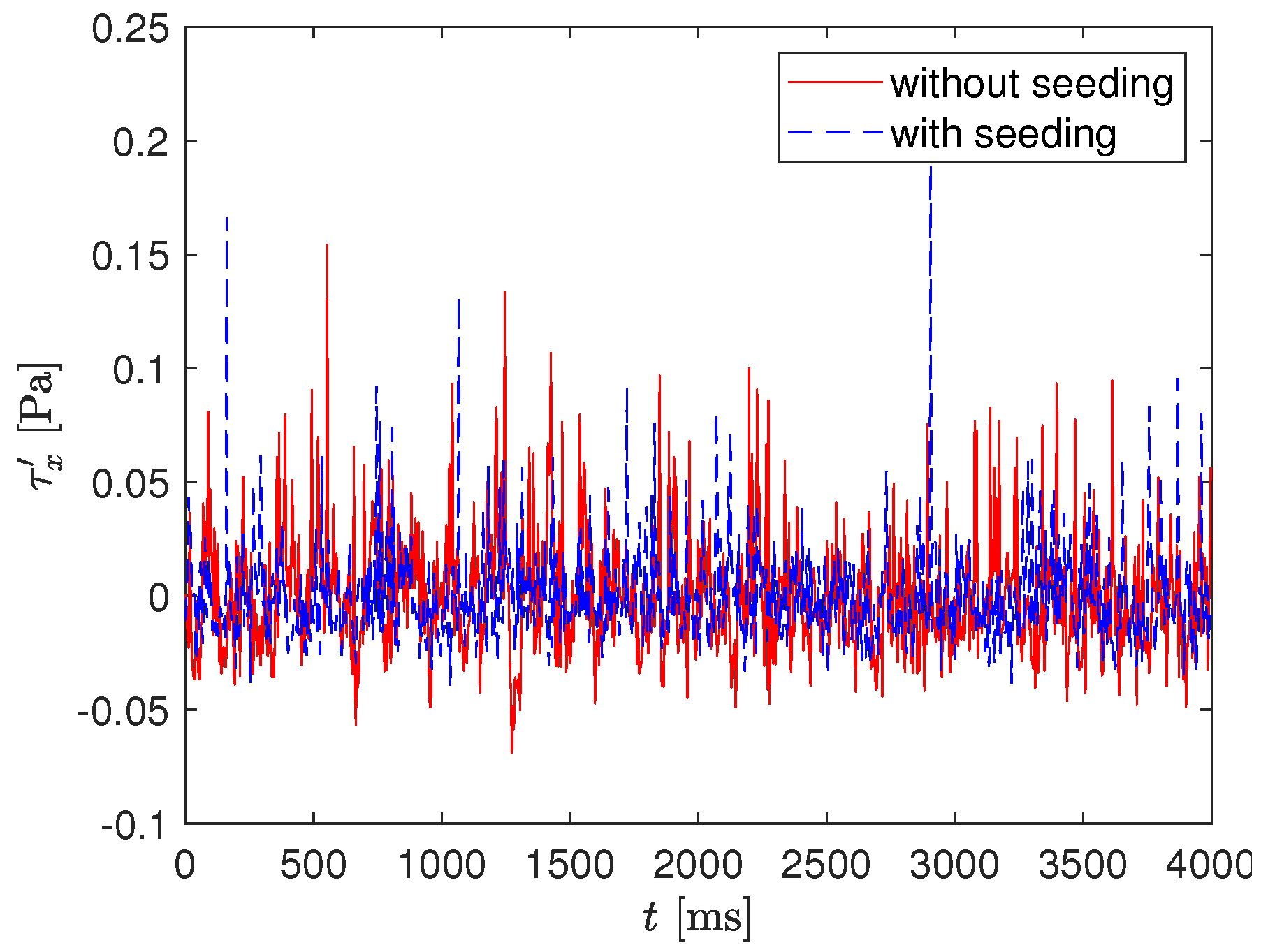
This theoretical, additional micro-pillar deflection was only occasionally observed in the recorded images. Figure 2 compares the time-dependent WSS fluctuations in streamwise direction of one representative micro pillar with and without seeding particles in the flow. The recording frequency was reduced to $f=250$ Hz to obtain a statistically meaningful dataset. The fluctuations around the baseline are in the same order of magnitude for both configurations, leading to the conclusion that the typical micro-pillar deflection is not influenced by the seeding particles. Nevertheless, a few exceptionally high deflections occur when seeding particles are present, e.g., at $t=2896$ ms, but they can easily be detected and as such eliminated. The local WSS was then calculated based on the neighboring values. Both measurements also showed a few major deviations, which probably arose from debris colliding with the micro pillar.

Another important influence of the seeding particles might arise from the added mass of the seeding fluid if it sticks to the micro pillar after collision. However, the mass of one seeding particle is five orders of magnitude smaller compared to the micro-pillar mass. Thus, its influence is theoretically negligible and, additionally, no damping of the micro-pillar response is visible in the WSS fluctuations, which would arise from, e.g., the added mass. In addition, no pollution of the MPS${}^3$ by seeding fluid was optically observed during the experiments. By storing one sample in DEHS for one week, tensile tests showed no variation of the Young’s modulus compared to a reference sample. Furthermore, no illumination of near-wall seeding particles by the LED system was noticed which could have affected the quality of the MPS${}^3$ images. It is necessary to make sure that the PIV measurement plane is not oriented too close to the MPS${}^3$ since the heat generation of the laser light sheet leads to an increased Young’s modulus, which, in turn, modifies the micro-pillar flexibility. Succeeding MPS${}^3$ measurements with and without seeding and laser operation did not show a noticeable influence of both components for the current location of the measurement plane.

In the following, the investigation of the near-wall small-scale dynamics and the imposed footprint by the outer LSM is presented. This analysis includes exemplary snapshot results as well as a statistical evaluation of the inclination angle.

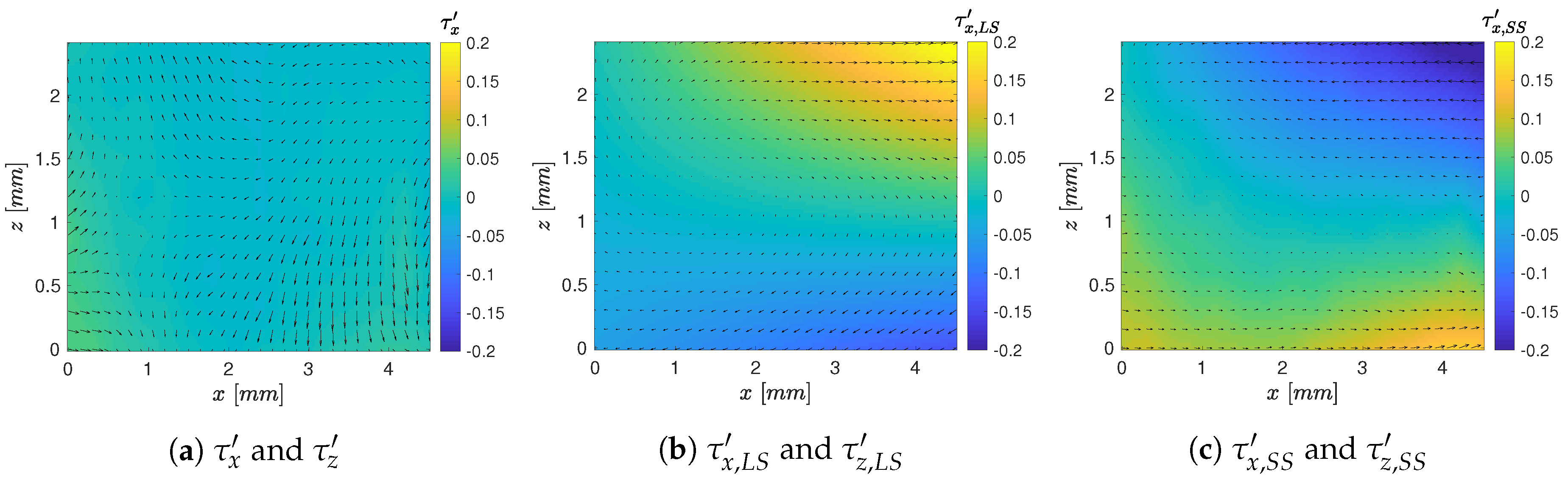
The mean WSS obtained by the MPS${}^3$ measurements measures ${\tau }_w=0.1094$ Pa. This value corresponds well to the theoretical WSS of a fully developed TCF ${\tau }_{w,theor}=0.1125$ Pa at $R{e}_{\tau }=969$. Figure 3 shows exemplary total (Figure 3a), large-scale (Figure 3b), and small-scale (Figure 3c) WSS fluctuations for a representative snapshot. The scales are separated by a two-dimensional EMD individually performed for the streamwise (${\tau }_x^{\prime }$) and the spanwise direction (${\tau }_z^{\prime }$). The color contours represent the corresponding fluctuations in the streamwise direction and the fluctuations in both directions are pictured by vectors. A comparison of the figures reveals that the large-scale and the small-scale WSS fluctuations possess the same order of magnitude. For the presented time step, the structures feature fluctuations with a very strong opposing amplitude, which cancels out for the total WSS fluctuations.

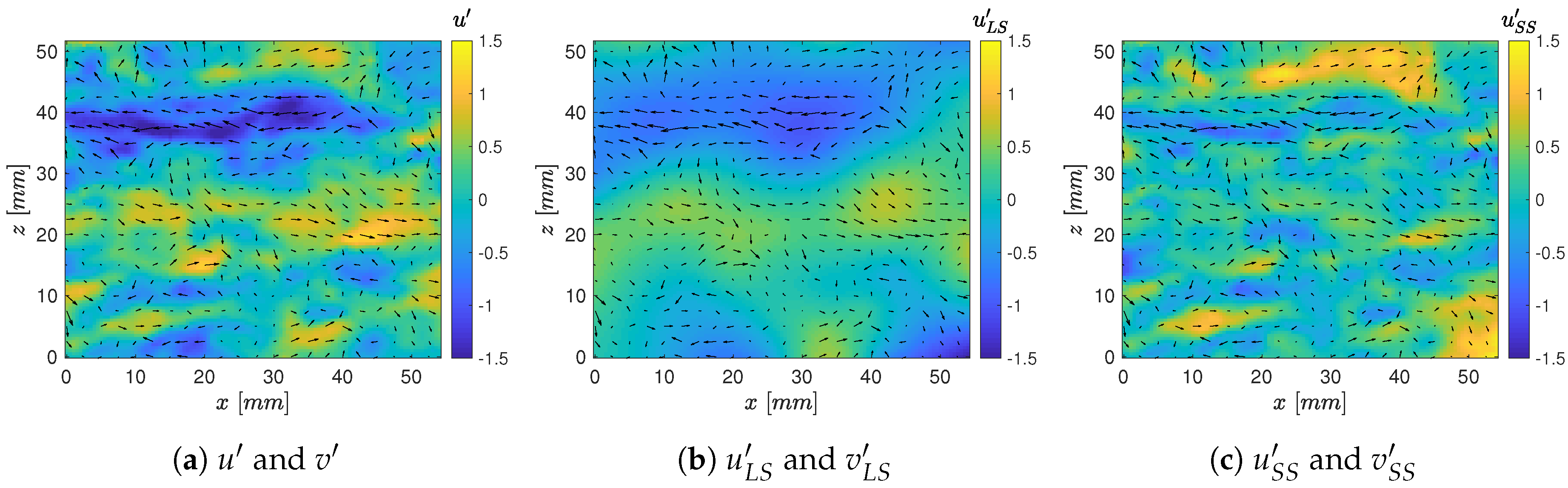
The velocity fluctuations in the outer layer obtained for the time step shown in Figure 3 using the PIV measurements are displayed in Figure 4. Again, the total (Figure 4a), the large-scale (Figure 4b), and the small-scale fluctuations (Figure 4c) are shown. Streamwise fluctuations are pictured by the color contours and the vectors represent the fluctuations in both directions, i.e., $u^{\prime }$ and $v^{\prime }$. For clarity, only every fifth vector is plotted. As for the WSS distribution, the magnitude of small- and large-scale fluctuations is similar. The total velocity fluctuations are qualitatively just a representation of the small-scale fluctuations magnitude-modified by the large-scale fluctuations. Figure 4b shows that a fast LSM meanders centrally through the field of view and is confined in the spanwise direction by two slow LSM. Since the field of view in the streamwise direction is smaller than $3h$, it is not possible to distinguish between LSM and very large-scale motions (VLSM) [33]. However, VLSM typically have a spanwise spacing of at least $1.3h$ [34,35]. Since the structures captured here feature a considerably smaller spacing, they are very likely to be LSM. At the small scales, which are shown in Figure 4c, slow and fast structures are alternating in the spanwise direction with a spacing of $\Delta z_{sp}=$ 10–15 mm $=$ 0.2–0.3 h or $\Delta z_{sp}^{+}=$ 181–271 in viscous scaling.

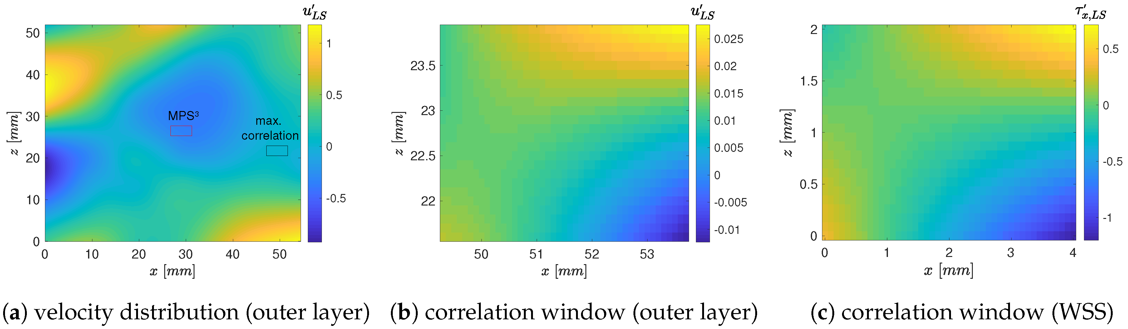
To investigate the footprint of the outer LSM imposed onto the near-wall small-scale WSS distribution, a cross-correlation between the large-scale components was performed. Figure 5 exemplarily shows the result of one time step. In Figure 5a, the large-scale streamwise velocity fluctuation field is pictured. The segment featuring the highest correlation with the large-scale streamwise WSS distribution of this time step (Figure 5c) is framed and an enlarged view is shown in Figure 5b. In addition, for clarification, the position of the MPS${}^3$ is marked by a square in Figure 5a. For the considered time step, the maximum correlation coefficient measures $\alpha =0.9852$. It can be used to scale the near-wall influence of the large-scale streamwise velocity fluctuations at the position shifted by the inclination angle [18]. The distance in streamwise direction between the segment with the highest correlation and the position of the MPS${}^3$ was used to calculate the inclination angle of superposition, which equals ${\Theta }_x={15.43}^{\circ }$ for this time step. A mean value over 1000 images gives an averaged angle of ${\overline{\Theta }}_x={16.53}^{\circ }$. Note that Agostini and Leschziner [15] determined an inclination angle of ${\Theta }_x={12.5}^{\circ }$ based on DNS data of a TCF at $R{e}_{\tau }=1025$. The authors of [18,36] also observed inclination angles between approximately ${11}^{\circ }$ and ${15}^{\circ }$ in TBL flows at Reynolds numbers on the order of $\mathcal{O}\left({10}^3\right)$–$\mathcal{O}\left({10}^6\right)$ based on HWA measurements. This leads to the conclusion that the mean angle between the LSM and their footprint in the near-wall region is comparable in TBL flows and TCF, at least for the investigated Reynolds number.

Unlike HWA measurements, the current measurement setup is able to acquire a two-dimensional representation of the flow field. Hence, the investigation of the large-scale footprinting can also include the meandering nature of the LSM, i.e., a motion in the spanwise direction. When considering this additional spanwise shift in the cross-correlation between large-scale velocity and WSS fluctuations, the inclination angle averaged over 1000 images yields a mean value of ${\overline{\Theta }}_{xz}={13.92}^{\circ }$. Hence, due to the meandering of the LSM, pointwise estimations considering only the streamwise evolution of the spatial delay between LSM and their footprint might overpredict the inclination angle. Further studies will be conducted to prove this hypothesis.

6. Conclusions

An extended approach is introduced in which the time-resolved two-dimensional wall-shear stress (WSS) distribution is simultaneously acquired with the time-resolved two-dimensional velocity field in the outer layer of a fully developed turbulent channel flow at a friction Reynolds number $R{e}_{\tau }=969$. The WSS distribution is obtained with the micro-pillar shear-stress sensor (MPS${}^3$) and the velocity field is measured by high-speed stereo particle-image velocimetry measurements. It was observed that the seeding particles, which are needed to perform PIV measurements, only occasionally influence the micro-pillar deflection. Since the impact is characterized by non-physical high micro-pillar deflections, it can easily be eliminated in the post-processing.

The simultaneous measurements were used to investigate the footprints of LSM present in the outer layer of the flow on the small-scale near-wall dynamics, which, to the authors’ knowledge, has never been done before experimentally in TCF. Therefore, the velocity fluctuation field as well as the WSS fluctuations were decomposed into small- and large-scale components by two-dimensional empirical mode decomposition. The maximum correlation coefficient of a cross-correlation between the large-scale distributions revealed the spatial delay in streamwise direction between the LSM and their near-wall footprint. The delay was used to calculate the inclination angle, which measures ${\overline{\Theta }}_x={16.53}^{\circ }$ when averaged over 1000 time steps. This value is similar to the angles obtained by HWA measurements in TBL flows, e.g., by Marusic and Heuer [18] and Mathis et al. [36]. This leads to the assumption that the inclination behaves similar in TBL flows and TCF.

Due to the two-dimensionality of the investigated data, the spatial delay between LSM and their footprint can also include the spanwise shift, which results from the meandering of LSM. The mean value calculated over 1000 time steps shows that the inclination angle decreases to ${\overline{\Theta }}_{xz}={13.92}^{\circ }$ and suggests that one-dimensional estimates might overpredict the superposition angle. Nevertheless, further investigations at varying Reynolds numbers have to be performed in TCF to validate this assumption.

The data will be used in the future to further investigate the near-wall small-scale modulation by outer LSM. The types of influence that are not yet considered in the current analysis, i.e., amplitude and frequency modulation as well as distortions by sweeps and ejections, will be studied in detail. Additionally, subsequent experiments at different Reynolds numbers will be performed to investigate Reynolds number dependent features.