Design and Fabrication of Heat Exchangers Using Thermally Conductive Polymer Composite

Abstract

Polymer heat exchangers (HXs) are lightweight and cost-effective due to the affordability of raw polymer materials. However, the inherently low thermal conductivity (TC) of polymers limits their application in HXs. To enhance thermal conductivity polymer composites, two types of diamond powders, with particle sizes of 0.25 µm and 16.7 µm, were used as fillers, while Acrylonitrile Butadiene Styrene (ABS) served as the matrix. Composite polymer samples were fabricated, and their density and thermal conductivity were tested and compared. The results indicate that fillers with larger particle sizes tend to exhibit higher thermal conductivity. A polymer HX based on a Triply Periodic Minimal Surface (TPMS) structure was designed. The factors influencing the efficiency of polymer HXs were analyzed and compared with those of metal HXs. In polymer HXs, the polymer wall is the primary source of heat resistance. Additionally, the mechanical strength of 3D-printed polymer parts was evaluated. Finally, an HX was successfully fabricated using a polymer composite containing 50 wt% diamond powder via 3D printing.

1. Introduction

Polymer heat exchangers (HXs) are lightweight and cost-effective due to the affordability of raw materials. They also offer excellent resistance to corrosion, making them ideal for use in harsh environments. Advanced polymer 3D printing technologies, such as fused filament fabrication (FFF) or fused deposition modeling (FDM), enable the production of highly customized polymer heat exchangers at lower costs and faster speeds. Moreover, 3D printing facilitates the integration of Triply Periodic Minimal Surface (TPMS) structures into the heat exchanger core. A TPMS structure enhances heat transfer efficiency from liquid to the solid wall and also strengthens the polymer heat exchanger, improving its overall performance [1,2,3].

Despite these advantages, polymer heat exchangers (HXs) still face challenges. Polymers generally have lower thermal conductivity (TC) compared to metals like copper or aluminum. As a result, polymer heat exchangers may not be as efficient as their metal counterparts and are limited in applications where maximizing heat transfer is critical. Therefore, improving the thermal conductivity of polymer materials is essential.

To enhance thermal conductivity, high thermally conductive fillers such as diamond powder, carbon, or metal particles are added into 3D-printable polymers like Acrylonitrile Butadiene Styrene (ABS) to create thermally conductive polymer composites (TCPCs) [4]. These fillers enhance the overall thermal conductivity by forming a percolating network that facilitates thermal transport [5]. TCPCs combine the benefits of polymer matrices with the distinct properties of conductive fillers, offering a cost-effective and easy-to-process solution to increase polymer thermal conductivity. This approach has been gaining significant attention.

Several factors influence the properties of the composite, including the filler volume ratio, filler shape, alignment, the surface treatment of the filler, and its intrinsic conductivity [6,7]. Generally, the thermal conductivity of polymer composites increases with the filler volume fraction. A high filler aspect ratio can create a conductive network at a lower volume fraction due to a reduced percolation threshold [8,9].

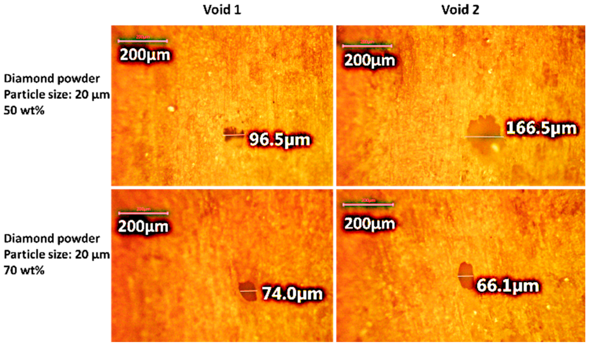
Filler particle size also plays a significant role in determining thermal conductivity. Polydisperse fillers generally exhibit higher thermal conductivity compared to monodisperse fillers [10]. Valeria et al. [11] found that composites containing 5 µm copper particles tend to have lower thermal conductivity than those with 150 µm copper particles. Li et al. [12] observed that smaller nanoparticles can lead to higher thermal conductivities due to their more widely spread aggregation structures in epoxy at the same concentration. The size effect of fillers at the nanoscale may differ from that of fillers at the microscale. While most studies focus on the effects of filler size at the micro level, further research on the impact of small filler sizes at the nanoscale is needed. Interfacial defects, such as voids or air gaps, increase thermal resistance by promoting phonon scattering [13,14,15]. The high interfacial thermal resistance between the filler and the polymer matrix is a key factor limiting the thermal conductivity of polymer composites [16]. The surface treatment of fillers can improve bonding with the polymer matrix, reducing interfacial flaws and thermal contact resistance.

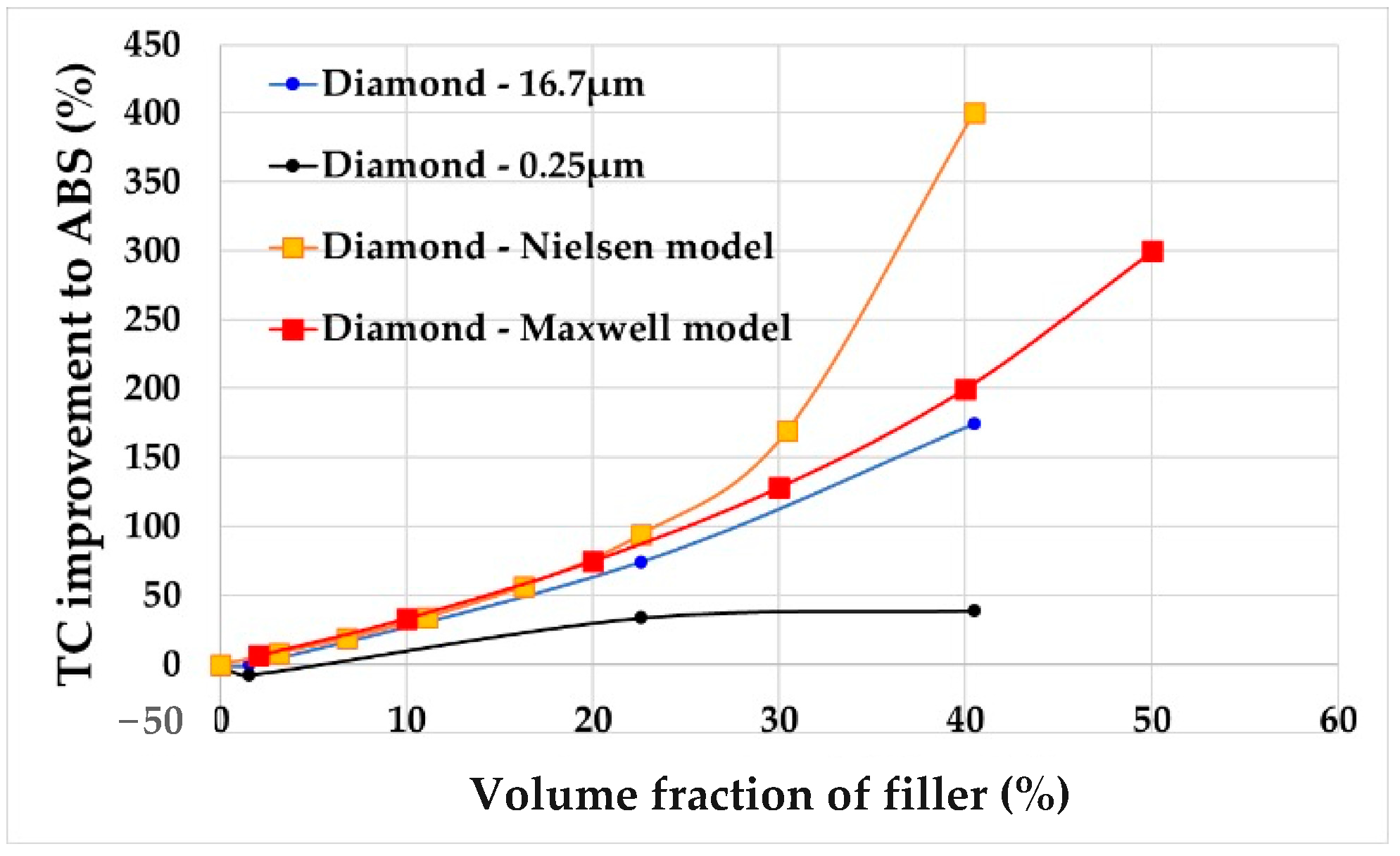
Several theoretical models have been developed to calculate the thermal conductivity of polymer composites. Maxwell [17] considered spherical particles with thermal conductivity $k_f$ embedded in a continuous matrix with thermal conductivity $k_m$, assuming a small volume ratio where the particles are far enough apart relative to their size. Maxwell proposed a formula to determine the effective thermal conductivity of the composite material, as shown below:

$$k_{eff}=k_m{\displaystyle \frac{k_f+2k_m+2\phi (k_f-k_m)}{k_f+2k_m-\phi (k_f-k_m)}}$$

(1)

Maxwell’s theory is accurate for a low filler volume ratio, typically up to around 25%.

Percolation theory [7,18] can be applied to understand the impact of filler volume fraction on heat transfer in polymer composites. The effective thermal conductivity of filled polymer composites can be determined using the following equation derived from percolation theory:

$$\lambda ={\lambda }_2{\left({\lambda }_c/{\lambda }_2\right)}^{{\left[{\displaystyle \frac{1-V}{1-V_c}}\right]}^n}$$

(2)

where ${\lambda }_c$ is the effective thermal conductivity of composites when $V=V_c$, and percolation exponent $n$ is dependent on the filler size, shape and distribution in the composites. ${\lambda }_2$ is the volume ratio. Once the filler volume ratio surpasses the percolation threshold, the thermal conductivity of the composite increases significantly with the filler volume ratio.

The thermal conductivity of polymer composites can also be estimated using the Nielsen theory [19]. The Nielsen model provides an accurate prediction of thermal conductivity up to approximately a 40% filler volume fraction and considers the effect of particle size.

$${\displaystyle \frac{K}{K_1}}={\displaystyle \frac{1+AB{\phi }_2}{1-B\mathrm{\varnothing }{\phi }_2}}$$

(3)

$$A=K_E-1$$

$$B={\displaystyle \frac{K_2/K_1-1}{K_2/K_1+A}}$$

$$\mathrm{\varnothing }=1+\left({\displaystyle \frac{1-{\phi }_m}{{\phi }_m^2}}\right){\phi }_2$$

$K$—thermal conductivity of the polymer composite;

$K_1$—thermal conductivity of matrix material;

$K_2$—thermal conductivity of filler;

$K_E$—generalized Einstein coefficient;

${\phi }_m$—the true volume of the particles divided by the volume they appear to occupy when packed to their maximum extent;

${\phi }_2$—volume fraction.

According to these theories, factors such as the volume ratio, filler aspect ratio and filler thermal conductivity influence the thermal conductivity of polymer composites.

ABS (Acrylonitrile Butadiene Styrene) is a common polymer filament used in 3D printing. The glass transition temperature (Tg) of ABS typically ranges between 105 °C and 120 °C (221 °F to 248 °F). The high Tg of ABS allows it to be used in application involving heat transfer from high-temperature liquids, such as water. Diamond has the highest thermal conductivity, which is about 2000 W/(mK), and is an excellent heat conductor. Moreover, diamond has isotropic properties of thermal conductivity.

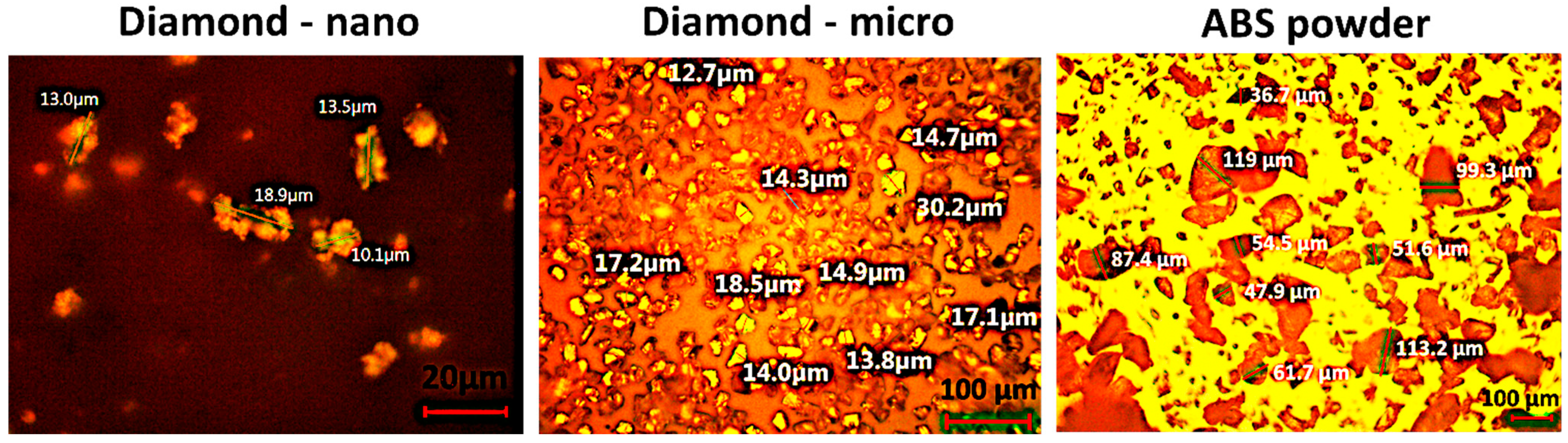
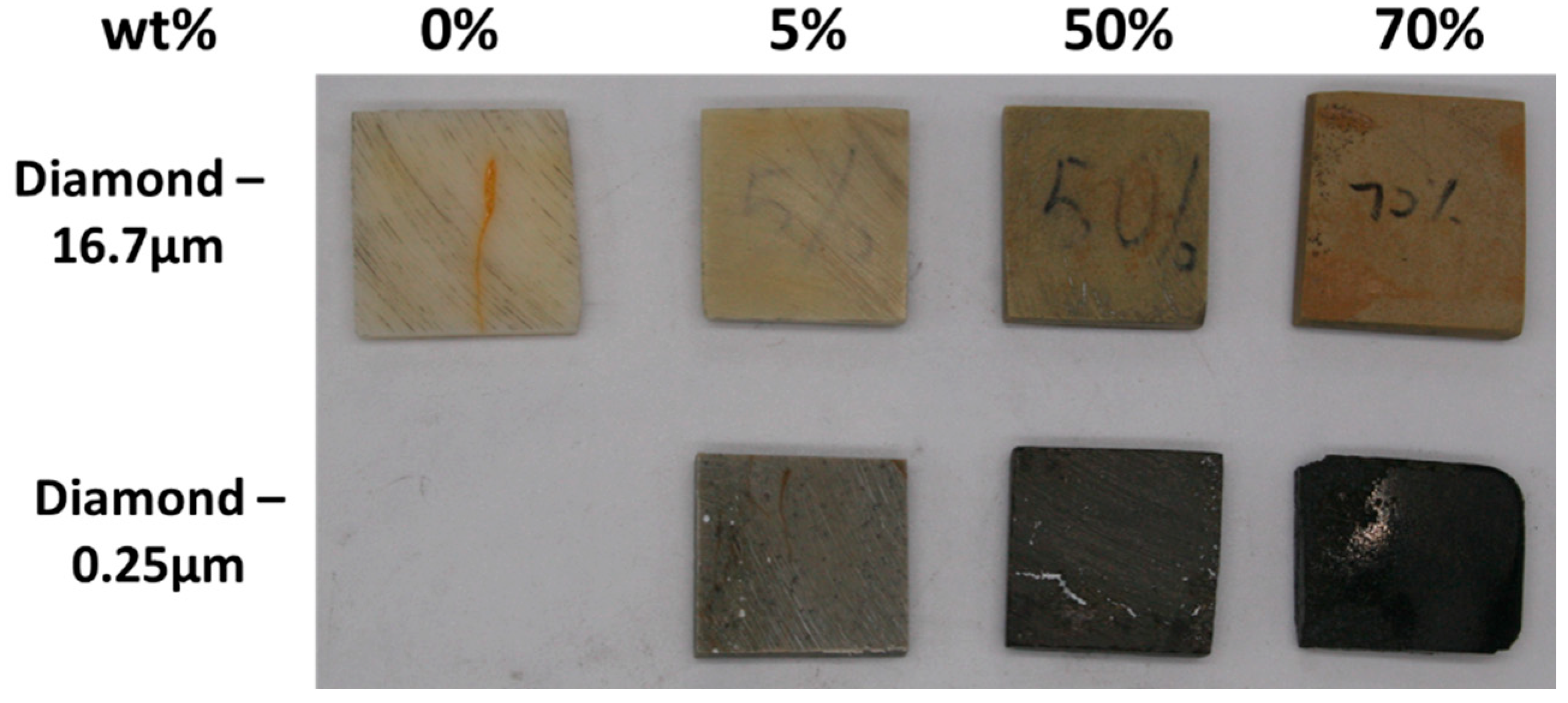
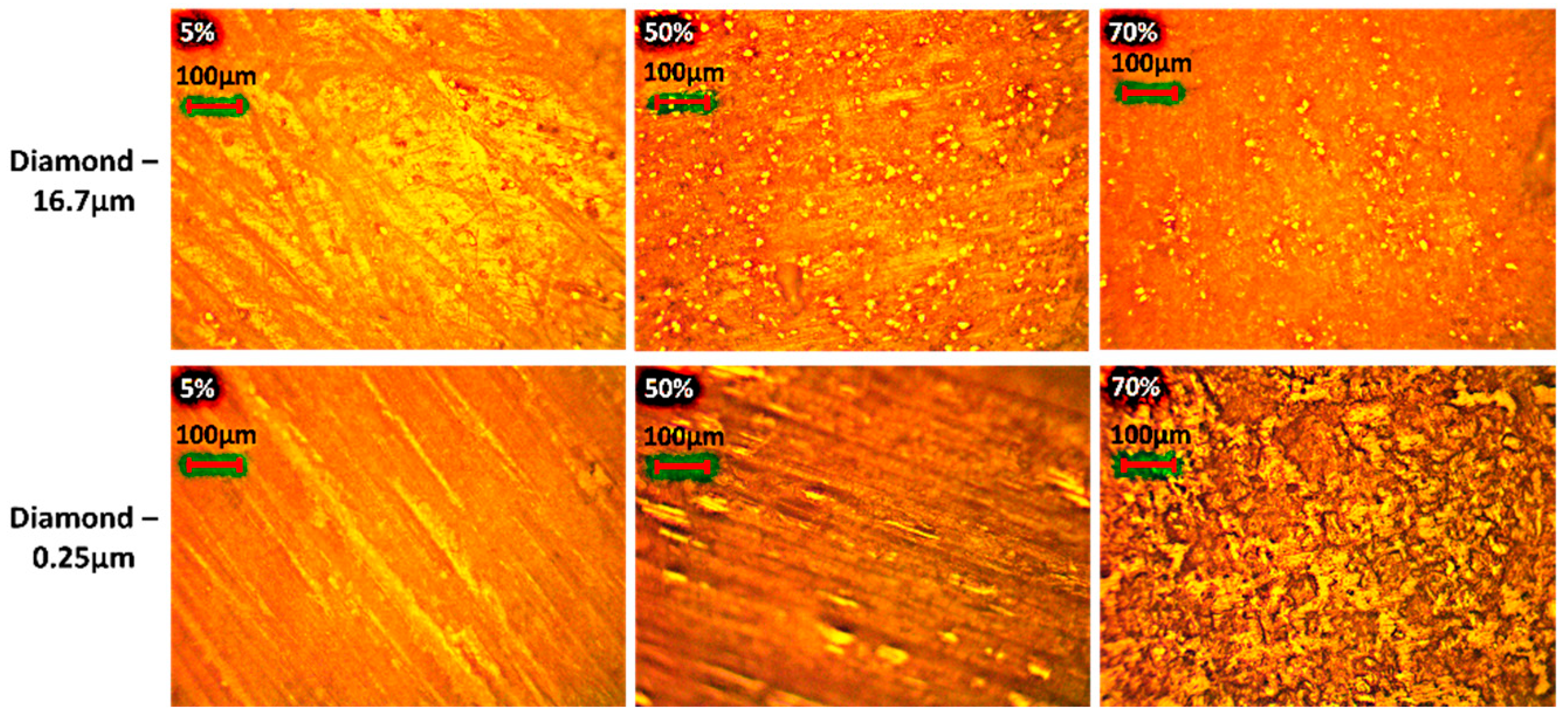
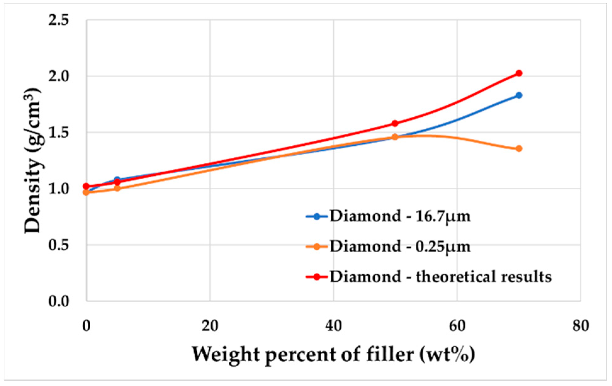
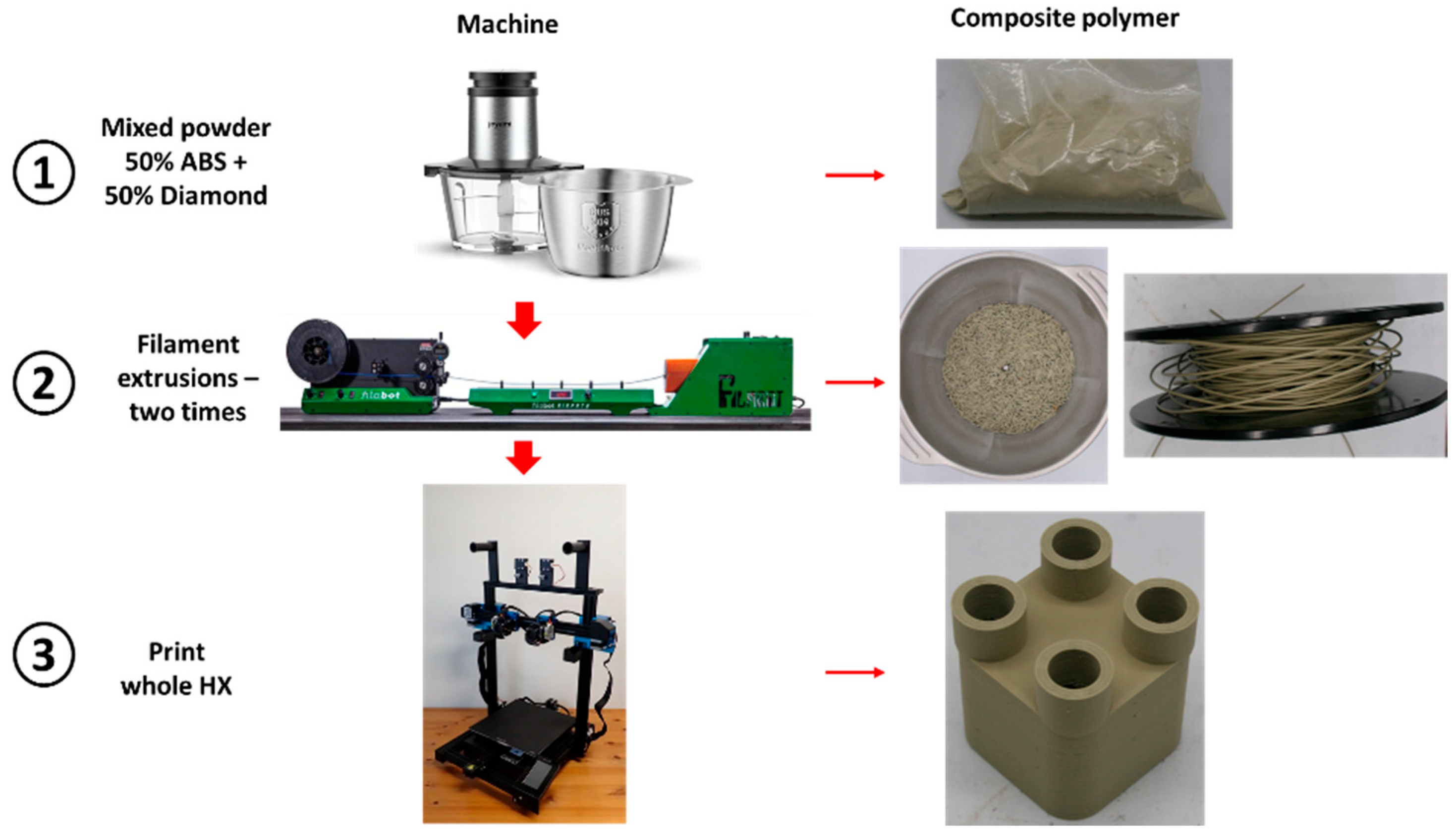
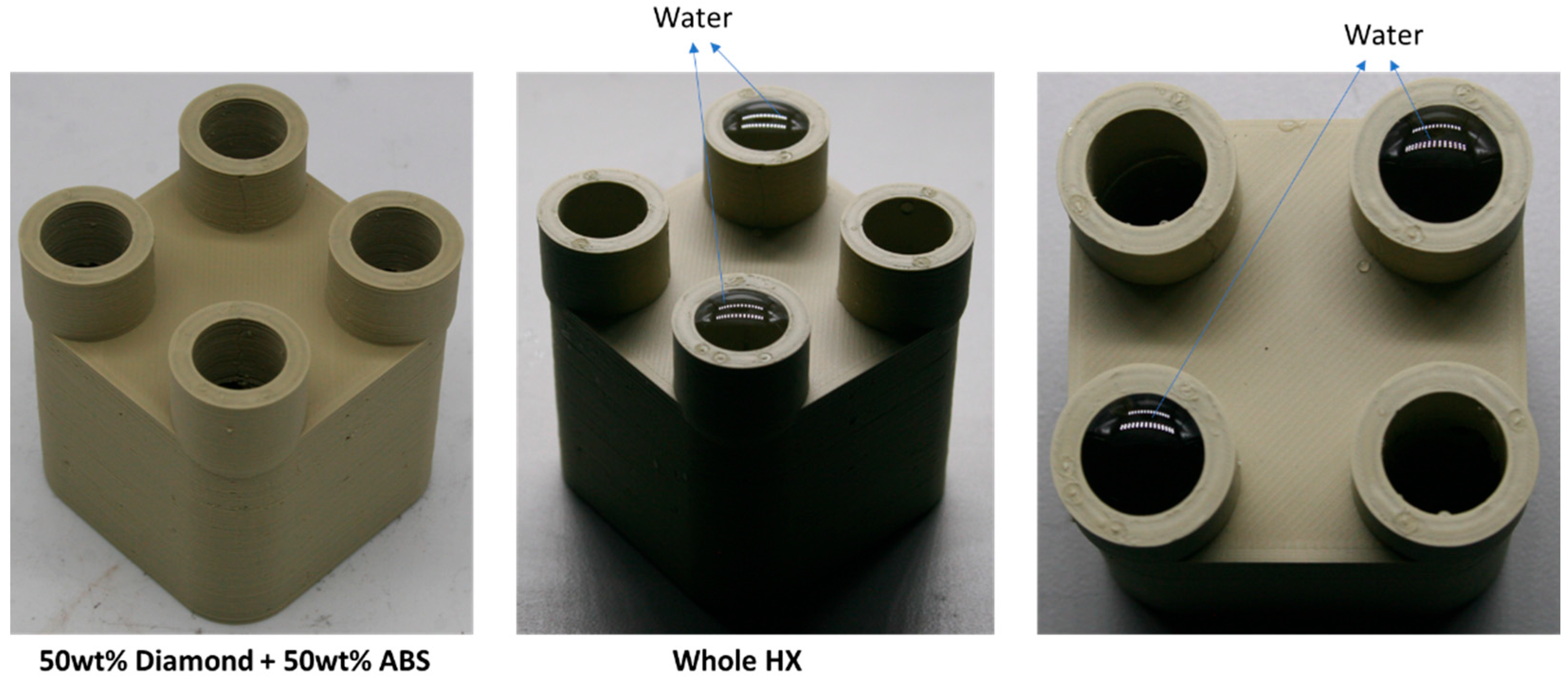
In this paper, diamond powder at both the nanoscale and microscale were used as fillers and added into ABS to create thermally conductive polymer composites (TCPCs). The density and thermal conductivity of two types of polymer composites were tested and compared. A heat exchanger (HX) model based on a gyroid lattice was designed and printed by a 3D printer. The heat transfer capacity of a polymer HX was evaluated through simulations and experimental testing. The results of the polymer HX were also compared with a metal HX. Key factors influencing the HX’s performance were analyzed. A mixed powder of 50 wt% ABS and 50 wt% microdiamond was extruded into filament. To enhance the filament quality, it was extruded twice. Using the extruded filament, a complete HX was successfully printed without any leakage. The mechanical strength of ABS polymer parts by 3D printing was tested.

Through the research in this paper, it has been demonstrated that adding fillers to the matrix can enhance the thermal conductivity of polymer composites. The experimental study also shows that nanometer-scale fillers do not significantly improve the thermal conductivity of polymer composites. The thermal conductivity of the polymer composites fabricated in this study still does not meet the practical requirements of heat exchangers. Further in-depth research on the relevant influencing factors is needed to improve the thermal conductivity of polymer composites. This study indicates that using a TPMS structure in polymer heat exchangers can improve heat transfer efficiency and reduce flow resistance. The internal flow channels of the polymer heat exchanger have a smoother surface, resulting in lower flow resistance compared to metal heat exchangers. This paper demonstrates the feasibility of the process by 3D printing a complete polymer heat exchanger using a polymer composite with a high weight fraction, proving the technological feasibility of this approach.

2. Investigation of Thermal Conductivity on Composite Polymer

2.1. Materials

ABS powder (150 mesh) was supplied by Magerial Science (Suzhou, China). Diamond powder was supplied by Signi Technology Ltd. (China).

As shown in Figure 1 and

Table 1. Properties of the filler and matrix.

	Unit	ABS	Diamond—Micro	Diamond—Nano
TC—solid	W/(m×K)	0.20	2000	2000
Density—Solid	g/cm3	1.02	3.5	3.5
Particle size—powder	µm	74.6	16.7	0.25

, the average particle size of microdiamond powder is 16.7 µm. The average diameter of ABS powder is 74.6 µm. Nanodiamond particles tend to aggregate, forming larger clusters. The average diameter of nanodiamond powder is 0.25 µm.

2.2. Samples of Polymer Composite

Square samples (20 mm × 20 mm × 5 mm) were fabricated by melting the mixed polymer composite in a molding box. The samples were then heat-treated in a high-pressure cooker for 30 min to remove the internal air bubble. The high-pressure cooker operates at high-pressure mode, at a temperature of 120 °C and a pressure of 200 kPa. After heat treatment, the density and thermal conductivity of the samples were measured.

As shown in Figure 2, three samples were created using a mixed powder containing microscale diamond powder with a particle size of 16.7 µm, with weight percent of 5%, 50%, and 70%, respectively. As the diamond content increased, the color of the samples became darker. Three samples were made using nanodiamond powder with a particle size of 0.25 µm, also at weight percentages of 5%, 50%, and 70%.

As shown in Figure 3, diamond particles with a size of 0.25 µm were too small to be visible under the microscope, suggesting that these particles were evenly dispersed in ABS.

2.3. Density of Polymer Composite

The density of pure ABS is 1.02 g/cm³ and the density of diamond is 3.5 g/cm³.

$${\rho }_c={\displaystyle \frac{1}{\frac{m_f}{{\rho }_f}+\frac{m_m}{{\rho }_m}}}$$

(4)

where ${\rho }_c$ is the density of polymer composite, $m_f$ is the mass fraction of filler, $m_m$ is the mass fraction of matrix, ${\rho }_f$ is the density of the filler, and ${\rho }_m$ is the density of the matrix.

As shown in Figure 4, the density of samples made from diamond powder with a particle size of 16.7 µm was nearly the same as that of samples made from diamond powder with a particle size of 0.25 µm particle size. As the weight percent of diamond powder increased, the difference between the measured and theoretical densities became bigger.

The variation in density suggests the presence of small voids in the polymer composite. As illustrated in Figure 5, microscopic analysis revealed small voids ranging from 60 to 200 µm in length in the samples containing 50 wt% and 70 wt% diamond powder.

2.4. Thermal Conductivity of Polymer Composite

The thermal conductivity of the samples was measured using the steady-state method, as shown in Figure 6.

During the testing, the temperature of the base was raised to $T_{plate}$, approximately 50 °C. As shown in Figure 6, thermal paste was applied to the interfaces between the steel cube, the sample, and the base. Additionally, the top surface of the steel cube was coated with thermal paste to enhance the accuracy of the test results obtained from the thermal camera. The thermal conductivity of square sample 1 can be calculated using the following equation:

$$K_{s1}={\displaystyle \frac{k_0{X}_{s1}(T_{s1}-T_e)}{T_{plate}-T_{s1}}}$$

(5)

In the equation, $k_0$ represents the heat transfer coefficient between the top surface of the sample and the surrounding air. The ambient air temperature is maintained at 20 °C, and the environment is still (no air movement). Therefore, $k_0$ is considered a constant. $K_{s1}$ represents the thermal conductivity of the material, $X_{s1}$ is the height of sample 1, and $T_{s1}$ is the temperature at the steel surface for sample 1. $T_e$ is the environmental temperature. For the other sample, sample 2, thermal conductivity $K_{s2}$ can be calculated using the equation below:

$$K_{s2}={\displaystyle \frac{k_0{X}_{s2}(T_{s2}-T_e)}{T_{plate}-T_{s2}}}$$

(6)

The room temperature is constant, which is 20 °C, and there is no wind in the room. Therefore, both sample 1 and sample 2 are subjected to the same conditions. Since the two samples have the same dimensions, coefficient $k_0$ is identical for both. $K_{s2}$ represents the thermal conductivity of sample 2, $X_{s2}$ is the height of sample 2, and $T_{s2}$ is the temperature at the steel surface for sample 2. The thermal conductivity ratio can be calculated using the equation below:

$${\displaystyle \frac{K_{s2}}{K_{s1}}}={\displaystyle \frac{T_{plate}-T_{s1}}{T_{plate}-T_{s2}}}\times {\displaystyle \frac{X_{s2}}{X_{s1}}}\times {\displaystyle \frac{T_{s2}-T\mathrm{e}}{T_{s1}-T\mathrm{e}}}$$

(7)

$T_{s1}$ and $T_{s2}$ are measured using a thermal camera after 30 min to ensure the samples have reached a steady thermal state. $X_{s1}$ and $X_{s2}$ are measured using a caliper. The ratio ${\displaystyle \frac{K_{s2}}{K_{s1}}}$ can then be calculated using the equation above. The temperature gap between the sample and the environment is big and ${\displaystyle \frac{T_{s2}-T\mathrm{e}}{T_{s1}-T\mathrm{e}}}$ is nearly 1. The term can be omitted. As shown in Figure 7, the temperature distributions of the two samples and base are different. The temperature difference indicates that the thermal conductivity of the two samples is different. The steady-state method is efficient, allowing for a quick comparison of the improvement in the thermal conductivity (TC) of the polymer composite with the base TC of the polymer.

The thermal conductivity of the samples is measured using the steady-state method. The test results are presented in

Table 2. Thermal conductivity of polymer composite with different fillers.

Filler	Filler Size	Weight Percent of Filler	Volume Fraction	${\mathit{T}}_{\mathit{p}\mathit{l}\mathit{a}\mathit{t}\mathit{e}}$	${\mathit{T}}_{\mathit{s}1}$	ΔT	Sample Height	Thermal Conductivity
mm	µm	wt%	vol%	°C	°C	°C	mm	W/(m×K)
Diamond	16.7	0	0	53.4	44.6	8.7	4.61	0.20
Diamond	16.7	5	2	52.9	42.8	10.1	5.32	0.20
Diamond	16.7	50	23	52.9	47.4	5.5	5.09	0.35
Diamond	16.7	70	40	53.4	49.3	4.0	5.83	0.55
Diamond	0.25	5	2	52.9	42.5	10.4	5.06	0.18
Diamond	0.25	50	23	52.9	45.8	7.1	5.00	0.27

and Figure 8.

As the density of diamond powder is 1.85 g/cm³, the maximum packing fractions of diamond powder ${\phi }_m$ = 0.53. The Nielsen model is represented by Equation (3), while the Maxwell model is represented by Equation (1).

As shown in Figure 8, diamond powder with nanoscale particles (0.25 µm) exhibits lower thermal conductivity at the same volume ratio compared to diamond powder with microscale particles (16.7 µm).

The effect of particle size on thermal conductivity was studied in [20]. In their paper, Moradi, S. et al. discussed the increase in thermal conductivity as the size of BN filler particles increased from 2 µm to 180 µm, considering the interface between the particles and the matrix. This interface acts as a barrier to heat flow. For specific filler content, the thermal conductivity measured in the reference paper is significantly higher than that reported in most other studies. Moradi, S. et al. achieved this by introducing a Lewis acid–base interaction between the filler and the matrix. The advantageous interactions between the thiol and the filler particles can reduce the thermal barrier at the interface, resulting in the higher thermal conductivity values.

For the diamond powder in this study, the ratio of area to volume is A/V = 6/D, where D is the diameter of the filler particle. The interface area of the filler particle is inversely proportional to particle size. For a given diamond volume ratio, smaller diamond particles have a larger interface area compared to larger particles, which could lead to higher thermal resistance at the interface. So, the thermal conductivity of a polymer composite with bigger particles is higher than that with smaller particles. Based on the test results, diamond fillers with larger particle sizes may result in higher thermal conductivity.

According to the theoretical results shown in

Table 3. Thermal conductivity of polymer composite predicted by Nielsen theory.

Diamond	ABS	Diamond	ABS	A	B	${\mathit{\phi }}_{\mathit{m}}$	$\mathit{\varnothing }$	$\mathit{K}$
wt%	wt%	vol%	vol%	Sphere	-	-	-	W/(m×K)
0	100	0	100	1.5	1.00	0.53	1	0.2
10	90	3	97	1.5	1.00	0.53	1.05	0.22
20	80	7	93	1.5	1.00	0.53	1.11	0.24
50	50	23	77	1.5	1.00	0.53	1.38	0.39
70	30	40	60	1.5	1.00	0.53	1.68	1.00

and Figure 8, the Maxwell results are relatively close to the experimental results. The results predicted by the Nielsen theory is much higher than the test results at a high filler volume fraction. As shown in Figure 3, the diamond particles were evenly distributed throughout the ABS and were almost completely unconnected to each other. This may explain why the Maxwell theory gives better prediction of thermal conductivity than the Nielsen model. The Nielsen model assumes that the filler will contact each other at a high volume fraction, which leads to a higher prediction about the thermal conductivity.

3. HX Modeling with Gyroid Lattice

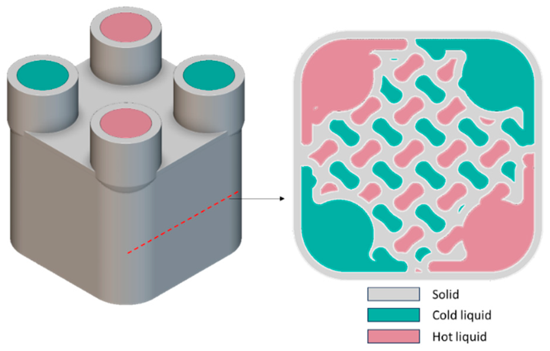
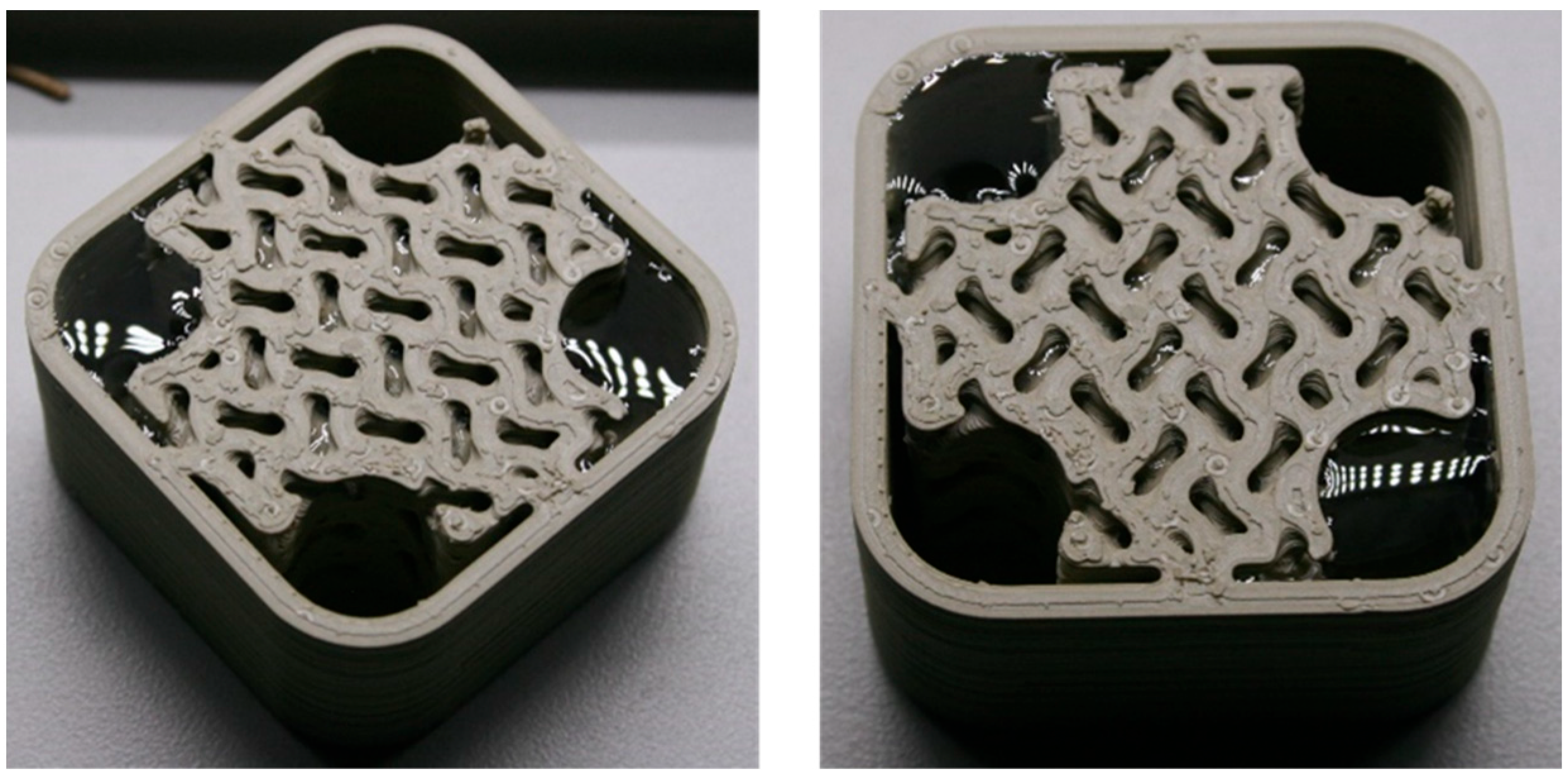
As shown in Figure 9, a polymer heat exchanger (HX) based on a gyroid lattice design was created. The HX consists of two volumes: one for cold water and the other for hot water. Heat is transferred from the hot water to the cold water. The gyroid lattice has dimensions of 12 × 12 × 12 mm, with a wall thickness of 2 mm. This design ensures that there is no leakage between the two volumes after printing.

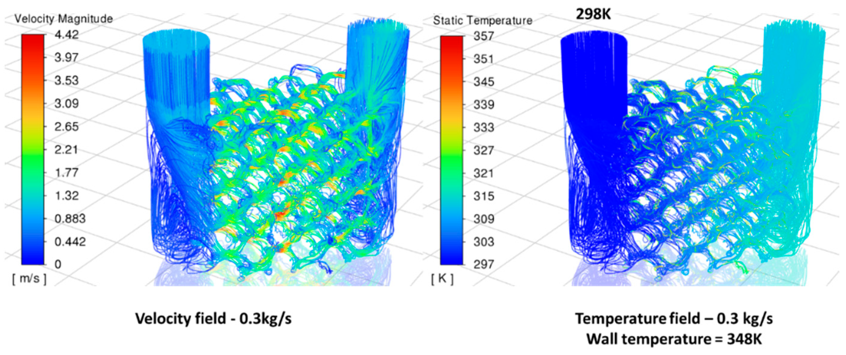
As shown in Figure 10, one fluid volume was calculated based on the symmetry of the two volumes. The inlet temperature of the water is 298 K, while the wall temperature of the lattice structure is maintained at a constant 348 K. The pressure drop and overall heat transfer coefficient of the single volume ($U_1{A}_1$) in the polymer HX were calculated through simulation.

The turbulence of the flow within the TPMS structure can be evaluated using the Reynolds number (Re), which represents the ratio of inertial forces to viscous forces and is defined as

$$Re={\displaystyle \frac{\rho V{d}_h}{\mu }}$$

(8)

where $\rho$ is the fluid density (kg/m³), $V$ is velocity in porous media (m/s), $\mu$ is the fluid viscosity (Pa.s), and $d_h$ is the hydraulic diameter. The definition of the hydraulic diameter employed in the TPMS structures is ${\displaystyle \frac{4\epsilon }{S_v}}$, where $S_v$ is the specific surface area (m²/m³). Porosity $\epsilon$ is defined as the fraction of the volume of voids over the total volume in the heat exchanger [21].

To calculate velocity $V$ in porous media, a cross-sectional plane at the midpoint of the heat exchanger along the flow direction within a control volume in ANSYS Fluent 2024 is created and the mean velocity across the section is calculated.

The thermal and hydraulic performance of heat exchangers can be evaluated using the Nusselt number (Nu).

$$Nu=U_1{\displaystyle \frac{d_h}{{\lambda }_f}}$$

(9)

where $U_1$ is the heat transfer coefficient of one volume, $A_w$ is the surface area between the interface of fluid and solid or total wetted surface area (m²), ${\lambda }_f$ is the fluid thermal conductivity (W/(m×K)).

For the simulation model, the heat transfer coefficient is calculated by the equation below:

$$U_1={\displaystyle \frac{q}{A_w\times \Delta T}}$$

(10)

$q$ is the heat transfer power;

$A_w$ is the surface area for heat transfer;

$T_{in}$ is the fluid inlet temperature;

$T_{out}$ is the fluid outlet temperature;

$T_{wall}$ is the temperature of the wall, which is constant.

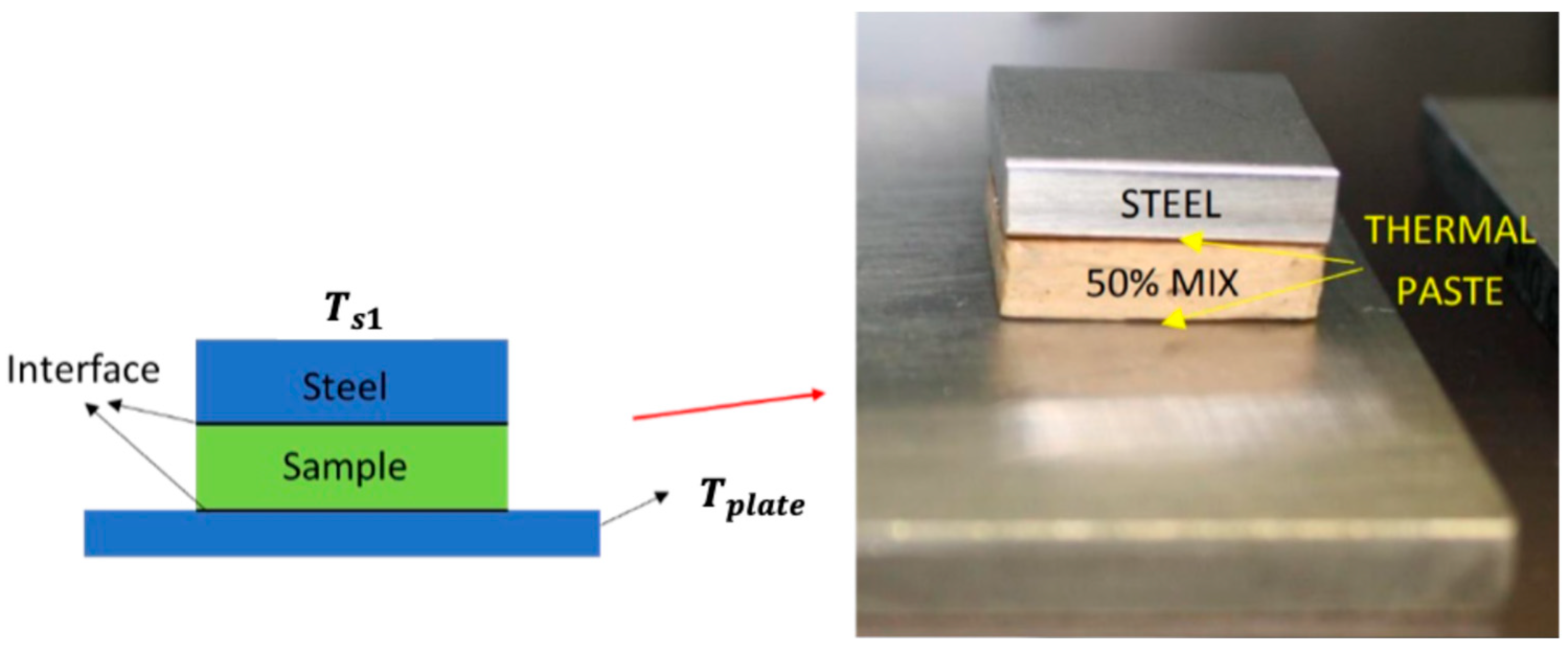
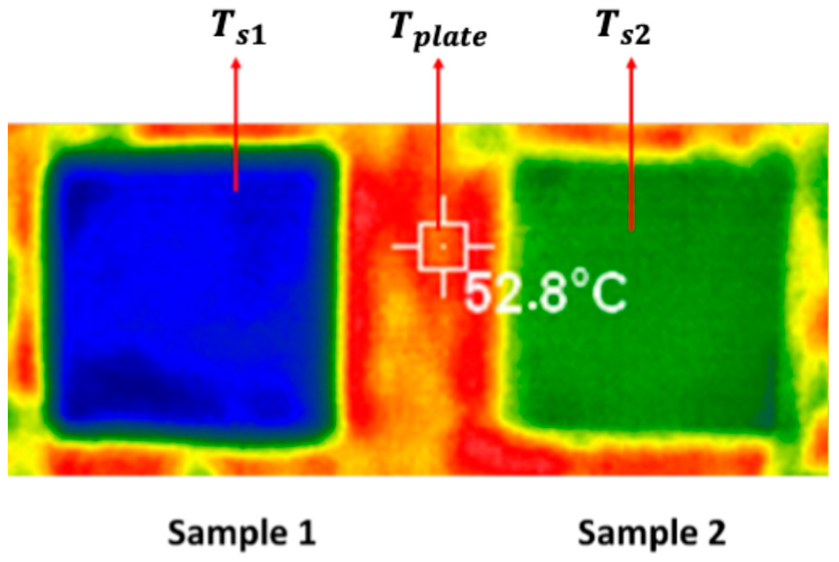
In the simulation, the temperature of the wall is set to be constant. The average temperature gap $\Delta T$ is represented by the equation below:

$$\Delta T=T_{wall}-{\displaystyle \frac{T_{in}+T_{out}}{2}}$$

(11)

For the test results, the heat transfer coefficient within a single volume can be calculated from the overall heat transfer coefficient using Equation (14), assuming that both volumes exhibit the same heat transfer coefficient due to the structural symmetry.

The friction factor ($f$) is commonly used to compare pressure loss in cooling channels and can be calculated using the following formula:

$$f={\displaystyle \frac{2\Delta p{d}_h}{\rho V^2{L}_c}}$$

(12)

where $\Delta p$ is the pressure loss in the system (Pa), and $L_c$ is the channel length (m) [21].

The Nu and f can be used together to evaluate the performance of the heat exchanger.

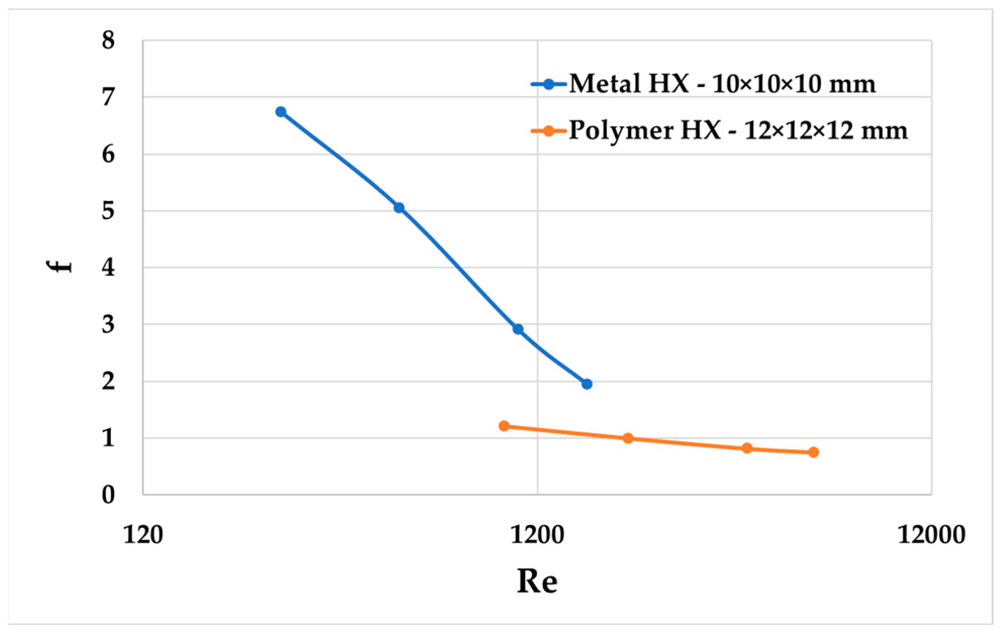
The metal heat exchanger (HX) in Figure 11 has the same dimensions as the polymer heat exchanger. The metal HX contains a lattice (10 × 10 × 10 mm) with a wall thickness of 1 mm in the core and is printed with AlSi10Mg powder, while the polymer HX has a larger lattice (12 × 12 × 12 mm) with a wall thickness of 2 mm. The Nusselt number (Nu) and friction factor (f) of the metal HX was calculated by the test results. Further details about the testing of the metal HX can be found in reference paper [1]. The Nusselt number (Nu) and friction factor (f) for the polymer HX was calculated by the simulation results. The pressure drop of the polymer HX at a flow rate of 0.2 kg/s was validated by the test results which are shown at

Table 4. Simulation results of the polymer HX.

${\mathit{A}}_{\mathit{w}}$	${\mathit{\delta }}_{\mathit{w}}$	Flow Rate	Inlet P	Reynolds	Nusselt Number	Friction f	${\mathit{U}}_1{\mathit{A}}_1$	$\mathbf{Thermal}\mathbf{Conductivity}\text{—}{\mathit{k}}_{\mathit{w}}$	Rw	${\mathit{U}}_{\mathit{c}}{\mathbf{A}}_{\mathit{w}}$
m2	mm	kg/s	Pa	Re	Nu	f	W/K	W/(m×K)	K/W	W/K
0.0252	2	0.05	580	991	41	1.21	178	0.20	0.42	2.34
0.0252	2	0.1	2018	2038	57	1.00	248	0.20	0.42	2.35
0.0252	2	0.2	6644	4098	84	0.81	364	0.20	0.42	2.37
0.0252	2	0.3	13,232	6038	106	0.75	457	0.20	0.42	2.38

and

Table 5. Test results of the polymer heat exchanger.

Cold Side Flow	Cold Side Pres Drop	Hot Side Flow	Hot Pressure Drop	Power
kg/s	Pa	kg/s	Pa	W
0.20	6045	0.20	5182	94

. The simulation result regarding pressure drop at 0.2 kg/s matches the test results. No correction factor is applied on the simulation results of the polymer HX.

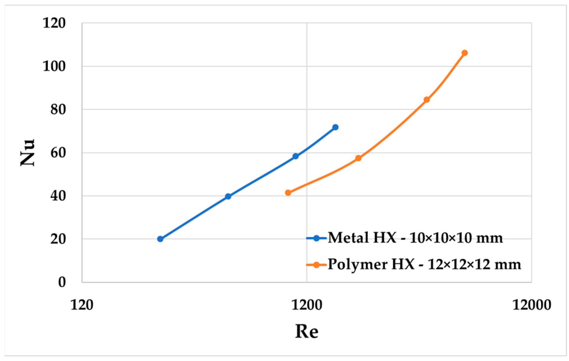
As shown in Figure 11 and Figure 12, an increase in friction factors at a low Re number in the metal HX was observed compared to the polymer HX. Nusselt numbers as functions of the Reynolds number in the metal HX had an upward and leftward shift across different Reynolds numbers compared to the polymer HX.

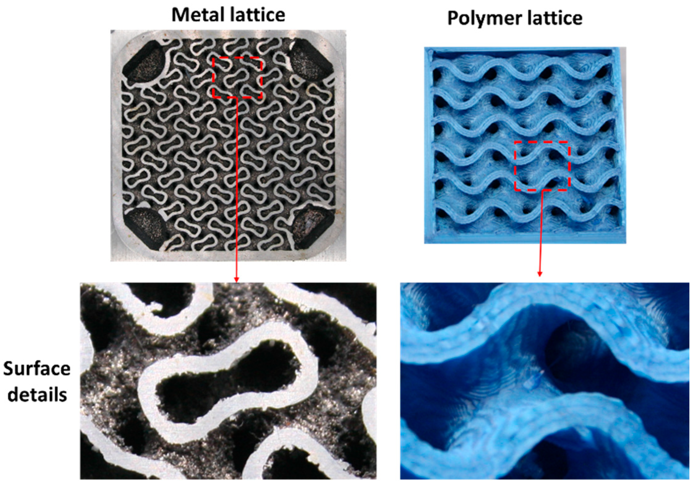
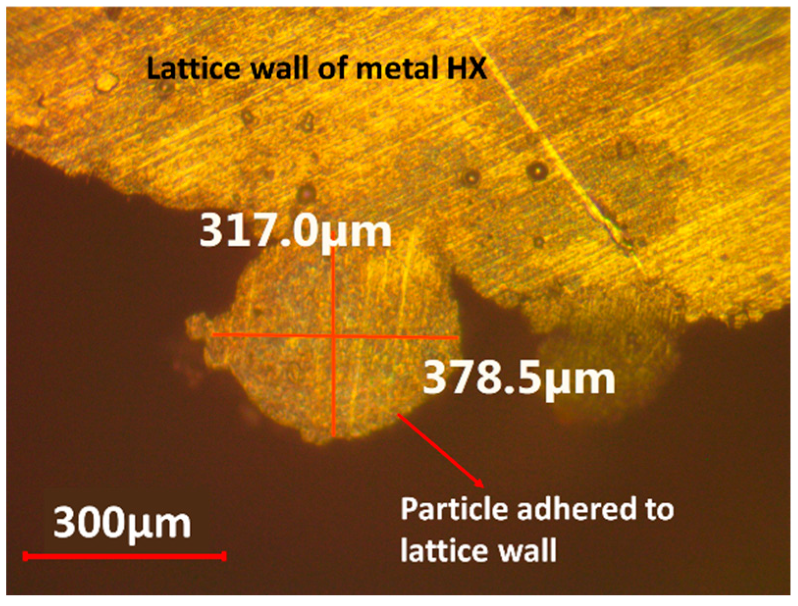
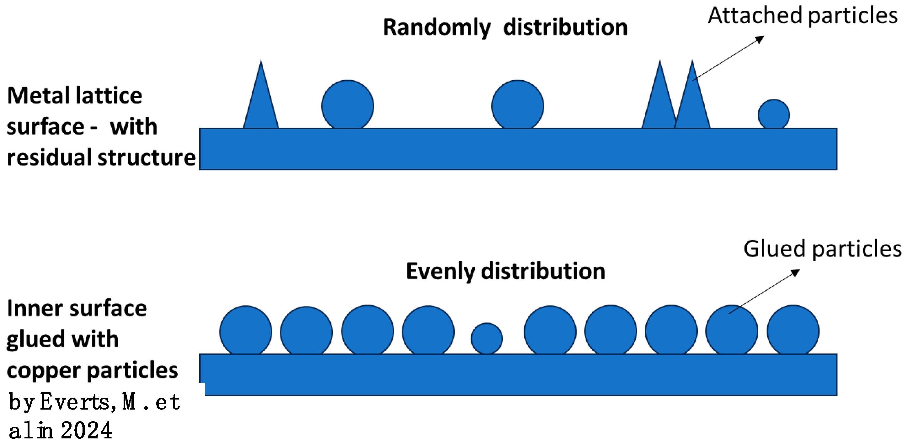
As shown in Figure 13 and Figure 14, a ball-shaped particle with a diameter of 350 µm was firmly attached to the lattice wall of the metal HX. Many particles of a similar size were adhered to the entire surface of metal lattice. Some of the attached particles resemble spikes, while others appear spherical. These particles are residual structures of 3D printing. The surface roughness of the metal lattice surface that do not have the attached particles is about 20 µm. The surface structure of metal lattice consists of areas with 20 µm roughness and the residual structures of 3D printing. The surface of the polymer lattice displayed several small stripes, but there were no residual structures on the surface.

Everts, M. et al. [22] investigated the impact of high relative surface roughness on heat transfer and pressure drop characteristics across different flow regimes through experimentation. To increase the relative surface roughness, Everts, M. et al. adhered small copper particles (150–300 μm) to the inner surface of the pipe, raising the surface roughness to 0.443 mm. The copper particles on the inner surface of the pipe are evenly distributed, as shown in Figure 15. The residual structures on the metal lattice surface after 3D printing is randomly distributed. It may not be accurate to state that the surface roughness of the metal lattice is the same to that of the inner surface of the pipe coated with copper particles, as reported in [22]. However, both the residual structures on the 3D-printed surface and the copper particles adhered to the inner surface of the pipe can disrupt the flow field around them, leading to an increased pressure drop and improved heat transfer efficiency. Some findings from the reference paper can help explain the variations in Nu and f with different Re values in the metal HX and polymer HX, as shown in Figure 11 and Figure 12.

Everts, M. et al. [22] also found that both the friction factors and Nusselt numbers as functions of the Reynolds number showed a clear upward and leftward shift as the relative surface roughness increased from 0.04 to 0.11. As shown in Figure 11 and Figure 12, the Nusselt number and friction factors also have an upward and leftward shift. Considering the surface comparison in Figure 13 and Figure 15, it is possible that the difference in Nu and f in the metal HX and polymer HX was caused by the residual structures of 3D printing on the lattice surface for the metal HX. Ongoing research is being conducted to study the effect of the residual structures of 3D printing.

The wall thermal resistance in polymer HX is given by

$$R_w={\displaystyle \frac{{\delta }_w}{k_w{A}_w}}$$

(13)

where ${\delta }_w$ is the thickness of the wall, $k_w$ is the thermal conductivity of the wall and $A_w$ is the heat transfer area of the wall, which is the same as $A_1$ or $A_2$ in this case [23].

The heat exchanger overall heat transfer coefficient [23]:

$$U_c{A}_w={\displaystyle \frac{1}{\frac{1}{U_1{A}_1}+R_w+\frac{1}{U_2{A}_2}}}$$

(14)

For the polymer HX, the pressure drop and $U_1{A}_1$ are provided in Table 4 and the other volume yields the same results due to its symmetry. The overall heat transfer coefficient $U_c{\mathrm{A}}_w$ of the entire heat exchanger is calculated using Equation (14). When the thermal conductivity is 0.20 W/(m×K), $U_c{\mathrm{A}}_w$ is approximately 2.35 W/K, which is relatively low. The small $U_c{\mathrm{A}}_w$ is attributed to the low thermal conductivity of the wall material. The polymer wall is the primary source of heat resistance.

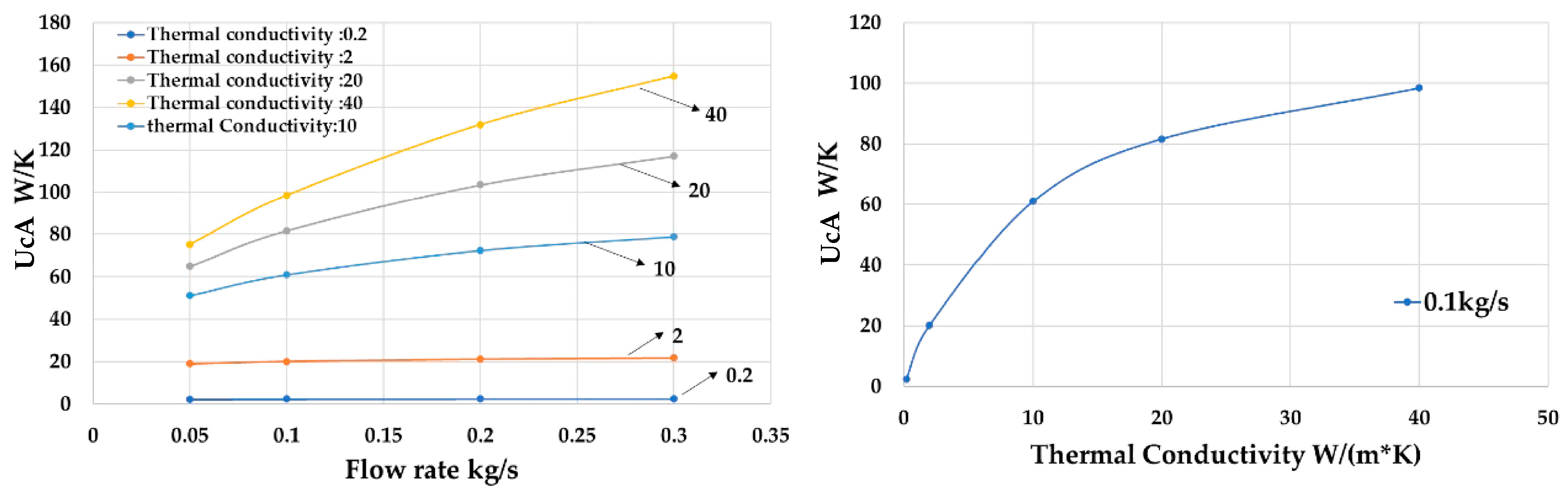
As shown in Figure 16, when the thermal conductivity of the material increases from 0.2 to 10 W/(mK), $U_c{\mathrm{A}}_w$ changes. However, when the thermal conductivity of the material increases from 20 to 40 W/(mK), the rate of increase in $U_c{\mathrm{A}}_w$ slows down. This suggests that the impact of thermal conductivity on the overall heat transfer performance of the polymer heat exchanger diminishes at higher conductivity values.

The test rig for the HX is described in [1]. During testing, the inlet temperature of hot water was 50 °C, and the inlet temperature of the cold water was 18 °C. The test results are provided in Table 5. The pressure drop was close to the simulation results. The simulated heat transfer power at the tested flow rate is approximately 76 W, while the measured heat transfer power is 94 W, which is in good agreement with the simulation. To improve the efficiency of the plastic HX, it is crucial to improve the thermal conductivity of the polymer material.

4. Three-Dimensional Printing of Polymer HX

4.1. Printing Procedures

As shown in Figure 17, the ABS powder and diamond powder were mixed using an electric food processor. The high-speed blade in the processor ensured the thorough blending of the two powders. An EX2 filament extruder was then used to extrude the filament from the mixed powder. The filament extruded for the first time was broken into small pieces, which were re-extruded again to obtain a high-quality filament. The entire HX was printed using a Sovol 04 3D printer, with the printing parameters provided in

Table 6. Printing parameters for the entire heat exchanger.

Print Temperature	Print Speed	Bed Temperature	Layer Height	Flow Rate
°C	mm/s	°C	mm	%
260	40	80	0.15	150

.

4.2. Mechanical Strength Testing of Polymer 3D Printing

The dimensions of the specimens that were used to test mechanical strength are shown in Figure 18, following the ASME E8 standard [24].

The printing directions listed in

Table 7. Mechanical strength of specimens produced by 3D printing.

Printing Direction	Dimension of Cross-Section in Middle	Max Force	Tensile Strength	Strain
-	Mm × mm	kN	MPa	%
Direction—1–0°	6.7 × 5.86	2.14	54	3.25%
Direction—1–45°	5.96 × 5.7	1.1	32	1.85%
Direction—2–0°	5.99 × 6.04	2.09	58	15%
Direction—2–45°	5.98 × 6.16	1.69	46	5.3%
Direction—3–0°	5.95 × 5.92	1.03	29	2.1%
Direction—3–45°	5.80 × 5.93	2.02	59	4.2%

are defined in Figure 19. Different printing directions may result in different tensile strengths. The material used to print the specimens is ABS.

As shown in Table 7, if the force direction aligns with the printing direction, the specimens have a higher tensile strength of approximately 55 MPa. When the force direction is at a 45 °C angle to the printing direction, the tensile strength is reduced to 60% of its original value. As shown in Figure 20, the printing direction plays a crucial role in maintaining the strength of the specimens. If the print is aligned with direction 2, the strain reaches its maximum value, which is approximately 15%.

4.3. Print of Entire HX

The entire HX was printed using a filament consisting of 50 wt% microscale diamond and 50 wt% ABS. The quality of the printed HX was excellent, with no water leakage between the two volumes. As shown in Figure 21 and Figure 22, the filament, containing 50 wt% diamond powder and 50 wt% ABS, was successfully used to print the complete HX structure.

5. Summary and Conclusions

In this paper, diamond powder was used as a filler and mixed with ABS powder to create polymer composites. The density and thermal conductivity of the polymer composites with varying filler weight percentages were measured and compared to the theoretical results. A polymer heat exchanger (HX) was designed and fabricated and its performance was simulated and compared to the experimental results. The factors affecting the performance of the polymer HX were analyzed. The entire HX was successfully printed using a composite polymer containing 50 wt% microscale diamond powder. The mechanical strength of the printed specimens was also measured. The conclusions are as follows:

• Improving the thermal conductivity of polymer composites is critical to HX performance.
• The thermal conductivity of polymer composites increases with the weight percent of the diamond filler.
• The fillers are distributed in the matrix evenly and result in isotropic TC properties.
• Nanoscale diamond particles do not significantly enhance the thermal conductivity of the composite polymer. Larger diamond particles contribute to higher thermal conductivity.
• The filament containing 50 wt% diamond powder can be successfully extruded, and the entire heat exchanger (HX) can be printed using this filament with a commercial 3D polymer printer.
• The residual structures from 3D printing on the lattice surface of a metal HX may result in an upward and leftward shift of the Nusselt number (Nu) and friction factor (f) as a function of the Reynolds number (Re) compared to the polymer HX.
• 3D-printed specimens have higher strength along the printing direction.

Further investigation is required to enhance the thermal conductivity of polymer composites. Based on the results presented in this article and relevant theories, effective approaches to increase the thermal conductivity include increasing the filler size, enhancing the aspect ratio of the filler, improving the surface energy, and using polydisperse fillers.

References

1. Liu, J.; Cheng, D.; Oo, K.; McCrimmon, T.-L.; Bai, S. Design and Additive Manufacturing of TPMS Heat Exchangers. Appl. Sci. 2024, 14, 3970. [Google Scholar] [CrossRef]
2. Liu, J.; Cheng, D.; Oo, K.; Pan, W.; McCrimmon, T.-L.; Bai, S. Optimization of Triply Periodic Minimal Surface Heat Exchanger to Achieve Compactness, High Efficiency, and Low-Pressure Drop. Energies 2024, 17, 5141. [Google Scholar] [CrossRef]
3. Huang, C.; Qian, X.; Yang, R. Thermal conductivity of polymers and polymer nanocomposites. Mater. Sci. Eng. R Rep. 2018, 132, 1–22. [Google Scholar] [CrossRef]
4. Li, Z.; Chen, X.; Liu, D.; Zhou, Y.; Pan, D.; Shin, S. Recent advances in polymer-based composites for thermal management and electromagnetic wave absorption. Adv. Compos. Hybrid Mater. 2025, 8, 210. [Google Scholar] [CrossRef]
5. Lebedev, S.M.; Gefle, O.S. Evaluation of electric, morphological and thermal properties of thermally conductive polymer composites. Appl. Therm. Eng. 2015, 91, 875–882. [Google Scholar] [CrossRef]
6. Hussain, A.R.J.; Alahyari, A.A.; Eastman, S.A.; Thibaud-Erkey, C.; Johnston, S.; Sobkowicz, M.J. Review of polymers for heat exchanger applications: Factors concerning thermal conductivity. Appl. Therm. Eng. 2017, 113, 1118–1127. [Google Scholar] [CrossRef]
7. Zhu, Y.; Chen, K.; Kang, F. Percolation transition in thermal conductivity of β-Si3N4 filled epoxy. Solid State Commun. 2013, 158, 46–50. [Google Scholar] [CrossRef]
8. Sanada, K.; Tada, Y.; Shindo, Y. Thermal conductivity of polymer composites with close-packed structure of nano and micro fillers. Compos. Part A Appl. Sci. Manuf. 2009, 40, 724–730. [Google Scholar] [CrossRef]
9. Wieme, T.; Duan, L.; Mys, N.; Cardon, L.; D’hooge, D.R. Effect of Matrix and Graphite Filler on Thermal Conductivity of Industrially Feasible Injection Molded Thermoplastic Composites. Polymers 2019, 11, 87. [Google Scholar] [CrossRef] [PubMed]
10. Shin, Y.K.; Lee, W.S.; Yoo, M.J.; Kim, E.S. Effect of BN filler on thermal properties of HDPE matrix composites. Ceram. Int. 2013, 39, S569–S573. [Google Scholar] [CrossRef]
11. Terentyeva, V.; Perera, I.U.; Narendran, N. Analyzing theoretical models for predicting thermal conductivity of composite materials for LED heat sink applications. In Proceedings of the IES Annual Conference Proceedings, Portland, OR, USA, 10–12 August 2017. [Google Scholar]
12. Li, X.; Park, W.; Chen, Y.P.; Ruan, X. Effect of Particle Size and Aggregation on Thermal Conductivity of Metal-Polymer Nanocomposite. J. Heat Transf. 2016, 139, 022401. [Google Scholar] [CrossRef]
13. Xu, Y.; Chung, D.D.L.; Mroz, C. Thermally conducting aluminum nitride polymer-matrix composites. Compos. Part A Appl. Sci. Manuf. 2001, 32, 1749–1757. [Google Scholar] [CrossRef]
14. Kochetov, R.; Korobko, A.; Andritsch, T.; Morshuis, P.; Picken Stephen, J.; Smit, J. Modelling of the thermal conductivity in polymer nanocomposites and the impact of the interface between filler and matrix. J. Phys. D Appl. Phys. 2011, 44, 395401. [Google Scholar] [CrossRef]
15. Khan, W.S.; Asmatulu, R.; Ahmed, I.; Ravigururajan, T.S. Thermal conductivities of electrospun PAN and PVP nanocomposite fibers incorporated with MWCNTs and NiZn ferrite nanoparticles. Int. J. Therm. Sci. 2013, 71, 74–79. [Google Scholar] [CrossRef]
16. Tan, J.; Zhang, Y. Thermally Conductive Polymer Composites: Recent Progress and Applications. Molecules 2024, 29, 3572. [Google Scholar] [CrossRef] [PubMed]
17. Maxwell, J.C. A Treatise on Electricity and Magnetism; Clarendon Press: Oxford, UK, 1881; Volume 1, pp. 398–404. [Google Scholar]
18. Mamunya, Y.P.; Davydenko, V.V.; Lebedev, E.V. Percolation Conductivity of Polymer Composites Filled with Dispersed Conductive Filler. Polym. Compos. 1995, 16, 319324. [Google Scholar] [CrossRef]
19. Nielsen, L.E. The thermal and electrical conductivity of two-phase systems. Ind. Eng. Chem. Fundam. 1974, 13, 17–20. [Google Scholar] [CrossRef]
20. Moradi, S.; Calventus, Y.; Román, F.; Hutchinson, J.M. Achieving High Thermal Conductivity in Epoxy Composites: Effect of Boron Nitride Particle Size and Matrix-Filler Interface. Polymers 2019, 11, 1156. [Google Scholar] [CrossRef] [PubMed]
21. Iyer, J.; Moore, T.; Nguyen, D.; Roy, P.; Stolaroff, J. Heat transfer and pressure drop characteristics of heat exchangers based on triply periodic minimal and periodic nodal surfaces. Appl. Therm. Eng. 2022, 209, 118192. [Google Scholar] [CrossRef]
22. Everts, M.; Mahomed, F. The effect of high values of relative surface roughness on heat transfer and pressure drop characteristics in the laminar, transitional, quasi-turbulent and turbulent flow regimes. Heat Mass Transf. 2024, 60, 1173–1193. [Google Scholar] [CrossRef]
23. Lee, H. Thermal Design: Heat Sinks, Thermoelectrics, Heat Pipes, Compact Heat Exchangers, and Solar Cells; John Wiley & Sons: Hoboken, NJ, USA, 2010. [Google Scholar]
24. American Society of Mechanical Engineers. ASME E8: Standard Methods for Tension Testing of Metallic Materials; ASME: New York, NY, USA, 2009. [Google Scholar]
Figure 1. Particle size of nanodiamond, microdiamond and ABS powder.
Applmech 06 00038 g001
Figure 2. Samples manufactured from various polymer composites.
Applmech 06 00038 g002
Figure 3. Microscopic images of the surfaces of various polymer composites.
Applmech 06 00038 g003
Figure 4. Density of polymer composites with varying weight percentages of diamond filler.
Applmech 06 00038 g004
Figure 5. Voids in polymer composite samples with diamond filler.
Applmech 06 00038 g005
Figure 6. Steady-state technique for measuring thermal conductivity.
Applmech 06 00038 g006
Figure 7. Temperature distribution tested by thermal camera for sample 1 and sample 2.
Applmech 06 00038 g007
Figure 8. Thermal conductivity of polymer composites with varying filler particle sizes.
Applmech 06 00038 g008
Figure 9. Design of polymer heat exchanger with dimensions 75 mm × 75 mm × 75 mm.
Applmech 06 00038 g009
Figure 10. Fluid flow simulation in the polymer heat exchanger.
Applmech 06 00038 g010
Figure 11. Friction factor as function of Reynolds number (Re) in polymer and metal heat exchangers.
Applmech 06 00038 g011
Figure 12. Nusselt number as function of Reynolds number (Re) in polymer and metal heat exchangers.
Applmech 06 00038 g012
Figure 13. Comparison of surfaces between metal lattice and polymer lattice.
Applmech 06 00038 g013
Figure 14. Small particles adhered to the lattice wall of the metal heat exchanger.
Applmech 06 00038 g014
Figure 15. The surface structure of the 3D-printed metal lattice and the pipe coated with copper particles [22].
Applmech 06 00038 g015
Figure 16. U c A of polymer heat exchanger with varying material thermal conductivity values.
Applmech 06 00038 g016
Figure 17. Fabrication procedures of entire heat exchanger—50 wt% diamond and 50 wt% ABS.
Applmech 06 00038 g017
Figure 18. Dimensions of specimen for tensile test.
Applmech 06 00038 g018
Figure 19. Specimens printed in different orientations.
Applmech 06 00038 g019
Figure 20. Stress and strain curve of specimens printed in different orientations.
Applmech 06 00038 g020
Figure 21. Leakage test of printed heat exchanger with 50 wt% microdiamond and 50 wt% ABS.
Applmech 06 00038 g021
Figure 22. Printed heat exchanger with 50 wt% microdiamond and 50 wt% ABS.
Applmech 06 00038 g022