Evaluation of Different Generative Models to Support the Validation of Advanced Driver Assistance Systems

Abstract

Validating the safety and reliability of automated driving systems is a critical challenge in the development of autonomous driving technology. Such systems must reliably replicate human driving behavior across scenarios of varying complexity and criticality. Ensuring this level of accuracy necessitates robust testing methodologies that can systematically assess performance under various driving conditions. Scenario-based testing addresses this challenge by recreating safety-critical situations at varying levels of abstraction, from simulations to real-world field tests. However, conventional parameterized models for scenario generation are often resource intensive, prone to bias from simplifications, and limited in capturing realistic vehicle trajectories. To overcome these limitations, the paper explores AI-based methods for scenario generation, with a focus on the cut-in maneuver. Four different approaches are trained and compared: Variational Autoencoder enhanced with a convolutional neural network (VAE), a basic Generative Adversarial Network (GAN), Wasserstein GAN (WGAN), and Time-Series GAN (TimeGAN). Their performance is assessed with respect to their ability to generate realistic and diverse trajectories for the cut-in scenario using qualitative analysis, quantitative metrics, and statistical analysis. Among the investigated approaches, VAE demonstrates superior performance, effectively generating realistic and diverse scenarios while maintaining computational efficiency.

1. Introduction

Automated driving (AD) technology is rapidly evolving, driven by substantial investments from leading technology companies and automotive manufacturers aiming to revolutionize transportation [1]. These advancements are driving the development of vehicles capable of navigating in complex environments autonomously, with automation levels ranging from basic driver assistance (level 1) to full autonomy (level 5) [2]. Level 3 systems, such as Mercedes-Benz’s Drive Pilot, can already handle specific driving tasks under defined conditions. The safe deployment of such systems relies on rigorous validation against a diverse array of challenging driving scenarios.

Scenario-based testing has emerged as an important methodology for validating the functionality and safety of Highly Automated Driving (HAD) systems [3,4]. By replicating real-world driving conditions, it provides a structured framework for assessing system performance in safety-critical situations. Traditional scenario-based testing, however, often relies on parameterized models to describe and simulate driving events [5,6]. While effective for basic scenarios, these models tend to oversimplify the complexity of real-world traffic, failing to capture the variability and unpredictability of actual driving environments. This limitation poses significant issues for thoroughly testing and validating the robustness of AD systems.

In response to these challenges, the automotive industry is increasingly turning to Artificial Intelligence (AI) methods to enhance scenario-based testing [7,8,9]. AI offers the capability to model complex, real-world scenarios more accurately by learning from large-scale driving data. Unlike traditional methods, AI can generate diverse synthetic scenarios that are both statistically consistent with observed data and reflective of the intricacy of actual driving environments. This approach not only improves the realism of scenario-based testing but also accelerates the development cycle by reducing the modeling effort.

Despite the application of AI techniques for scenario-based testing, generating realistic, diverse, and simulation-ready driving scenarios remains a challenging task. For example, the AE-GAN framework [7] focuses on reconstructing trajectory shapes without modeling full maneuver dynamics. Similarly, the BézierVAE approach [8] relies on drone-based data, limiting its ability to capture ego-centric driving interactions accurately. Multi-trajectory generators like MTG [9] primarily focus on generating short, disconnected sequences. These methods mainly rely on recurrent architectures or parametric curves. However, convolutional neural networks, which have shown strong performance in capturing spatial dependencies, remain underexplored for driving scenario generation.

In [10], the effectiveness of a Variational Autoencoder combined with a convolutional neural network (VAE) is demonstrated for generating realistic and diverse synthetic driving scenarios. This approach proves to be capable of learning and replicating the probabilistic structures of real driving behavior. Building on this foundation, the current study expands the focus by comparing the performance of GAN variations, which have demonstrated their superiority in applications like synthetic image generation and time-series modeling [11,12,13,14]. Other approaches, such as Normalizing Flows and Diffusion Models, although powerful for density estimation or sample refinement, are either less effective in capturing multi-modal diversity or computationally intensive for large-scale scenario synthesis. Given these considerations, we select three representative GAN variations that capture different strengths within adversarial learning: a basic Generative Adversarial Network (GAN) [15], known for its simple formulation, Wasserstein GAN (WGAN) [16], which offers better training stability, and Time-Series Generative Adversarial Network (TimeGAN) [14] designed to capture temporal coherence. By applying and evaluating these models in the present study, we aim to identify the most effective approach for generating realistic and diverse driving scenarios.

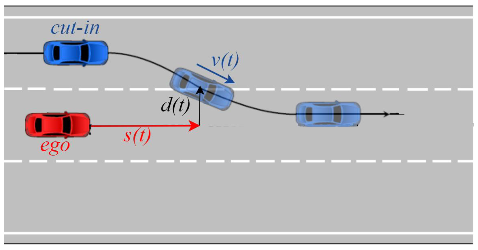
In this work, the focus is on the cut-in scenario, which is both common in real-world driving and widely regarded as one of the most challenging for scenario generation in simulation testing. The abrupt nature of cut-ins, coupled with their limited reaction time and high variability in driver behavior, makes them particularly difficult to model and replicate realistically. This high-risk event involves a vehicle abruptly entering the ego vehicle’s lane, requiring immediate action to avoid collision. It tests the ability of an automated system to adapt to sudden changes in traffic flow and dynamic conditions, making it a crucial benchmark for evaluating the decision-making capabilities. The generative models need to replicate cut-in scenarios while maintaining the temporal coherence and spatial fidelity of measured maneuvers.

The preparation of measured data for cut-in scenarios, as discussed in Section 2, involves filtering large-scale real-world driving datasets to extract relevant events. In particular, the lateral position and longitudinal velocity of vehicles are segmented for training the generative models and comparison. The explored generative models are detailed in Section 3, Section 4 and Section 5, while their training details and model efficiency are discussed in Section 6. Section 7 and Section 8 cover qualitative and quantitative analyses of the cut-in maneuvers generated by the models across three key dimensions: scenario realism, which evaluates how closely the generated scenarios align with real-world driving data; diversity, ensuring a broad representation of observed driving behaviors; and statistical similarity, which examines the model’s ability to capture stochastic properties such as trajectory likelihood and event duration.

2. Measured Cut-In Maneuvers

The models are trained using real-world measurement data collected during test drives. These measurements include Electronic Control Unit (ECU) signals from the ego vehicle and sensor data from surrounding objects, sampled at 50 Hz (0.02 s time interval). These high-resolution data capture critical parameters such as the relative longitudinal and lateral position $\left(s\right(t),d(t\left)\right)$ and absolute speed $v\left(t\right)$ of the vehicles in the surrounding, forming a comprehensive basis for scenario modeling and analysis [10].

A representative cut-in scenario is illustrated in Figure 1, where a neighboring vehicle merges laterally into the ego vehicle’s lane. To identify such scenarios, a two-step classification framework is implemented, combining rule-based classification with a Time-Series Forest (TSF) machine learning model. In [17], it is shown that TSF outperforms rule-based classification with respect to accuracy and robustness. By combining both methods, the system retains the efficiency of rule-based filtering while improving detection reliability with TSF.

Before being processed by the TSF classifier, the data undergo preprocessing, like the removal of dropouts and correction of curved roads as outlined in [10]. The final dataset comprises refined time-series data specifically tailored for training AI models to recognize and simulate cut-in scenarios. It consists of $N_S$ extractions, each containing $N_t$ time steps which provide a structured representation of vehicle motion over time. The key variables used in this investigation are the lateral position $d\left(t\right)$ and longitudinal velocity $v\left(t\right)$, both measured at discrete time points $t_k$ where $k=1\dots N_t$. Each extraction i forms a collection of measurements represented as

$$(t_k^{\left(i\right)},d_k^{\left(i\right)},v_k^{\left(i\right)}),i=1,\dots ,N_S,k=1,\dots ,N_t.$$

(1)

To separately analyze $d\left(t\right)$ and $v\left(t\right)$, their measurements are summarized in feature vectors

$${\mathbf{x}}_i={\left[\begin{array}{cccc}{x}_1^{\left(i\right)}& x_2^{\left(i\right)}& \dots & x_{N_t}^{\left(i\right)}\end{array}\right]}^{\top }\in {\mathbb{R}}^{N_t},x\in \{d,v\},i=1,\dots ,N_S.$$

(2)

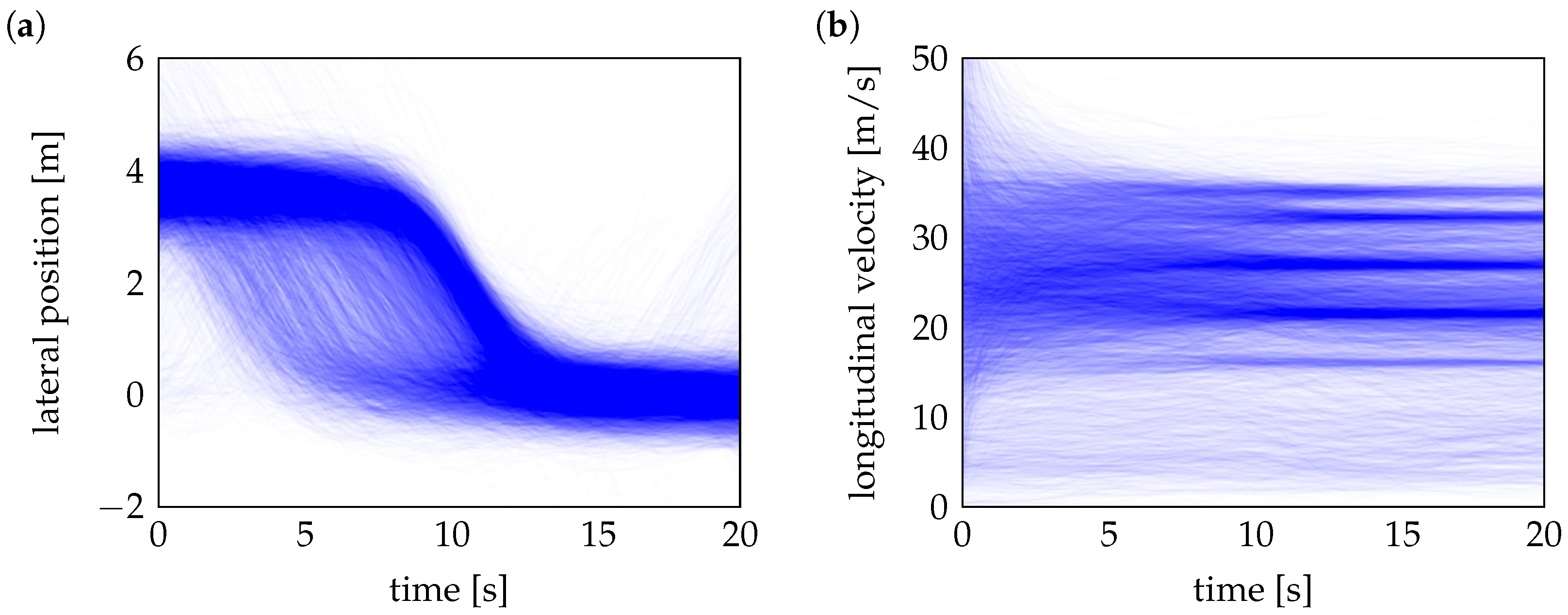
Figure 2 illustrates heatmaps of measured lateral positions ${\mathbf{d}}_i$ and velocities ${\mathbf{v}}_i$ for cut-in scenarios, derived from over 8000 real-world cut-in trajectories recorded by a vehicle fleet. The lateral position heatmap highlights high-density regions where cut-in maneuvers are the most frequently observed. These maneuvers typically start at a lateral offset of 3 to 4 m from the center of the ego vehicle’s lane, corresponding to the standard lane width on German highways. As the maneuver progresses, the vehicles perform a lane change and eventually stabilize near the center of the ego’s lane. Similarly, the velocity heatmap reveals that most cut-in events occur at speeds ranging from 20 m/s to 35 m/s, reflecting typical highway driving conditions.

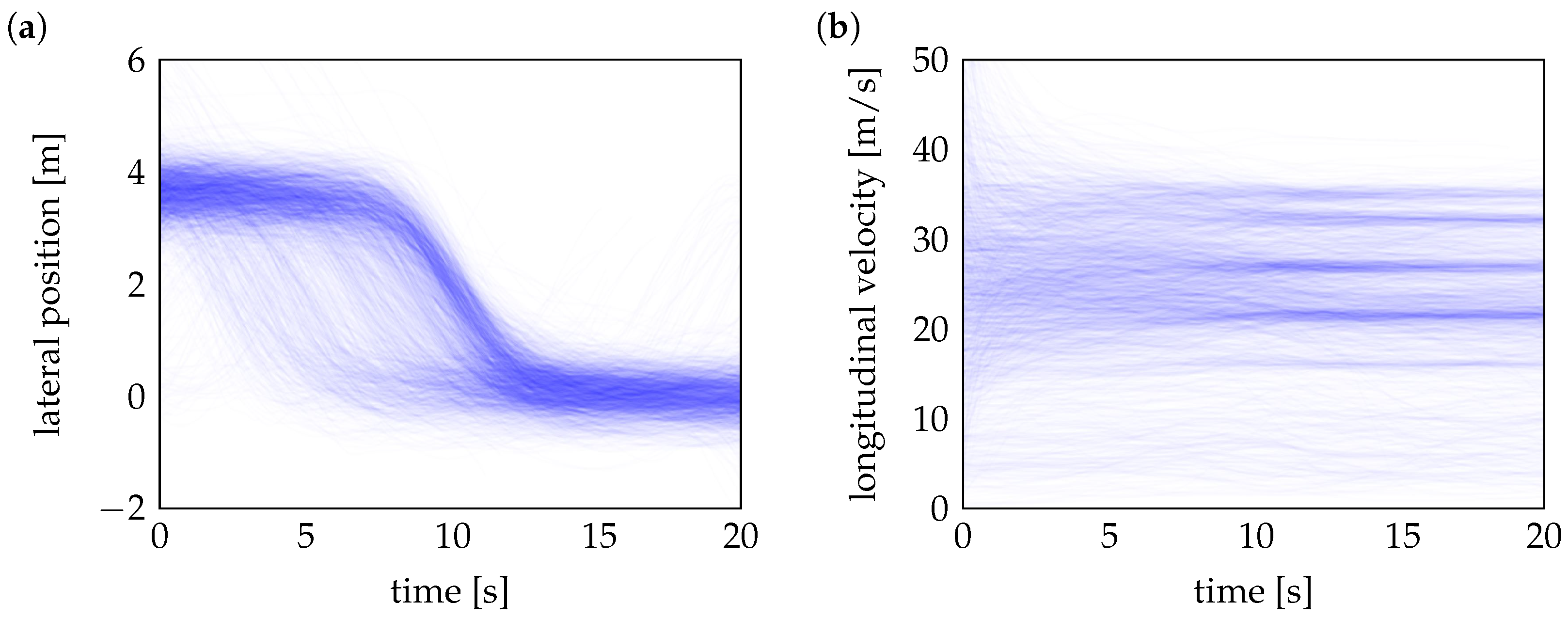
For training generative models, only a randomly selected 25% part of these measured cut-in maneuvers (approximately 2000 trajectories), as shown in Figure 3, is used. While initial experiments used a larger training split, the final experiments deliberately use a reduced subset to simulate a more challenging data-scarce environment. This setting allows to better evaluate the robustness and generalization capabilities of the generative models under limited data conditions, which are common in real-world autonomous driving applications. During evaluation, each model generates the same number of synthetic trajectories as the full set of measured cut-in maneuvers, and the generated scenarios are then compared to the original dataset to assess how accurately the models replicate real-world distributions.

3. Variational Autoencoder

Before introducing specific generative models, it is essential to clarify their primary goal. Generative models aim not just to replicate or approximate a given dataset but to learn the underlying probability distribution $p_x(\mathbf{x})$ of the measured data to enable the creation of new, diverse, and realistic maneuvers ${\tilde{\mathbf{x}}}_j$ from the learned generator probability distribution $p_g\left(\tilde{\mathbf{x}}\right)$. The generated maneuvers capture the essential statistical properties and variability present in the original data if $p_g\approx p_x$. In this work, the models are trained on observed cut-in maneuvers from real-world driving and learn to generate an arbitrary number of synthetic but realistic lateral positions ${\tilde{\mathbf{d}}}_j$ and longitudinal velocities ${\tilde{\mathbf{v}}}_j$ of trajectories that exhibit similar behavioral patterns to those seen in the measured data.

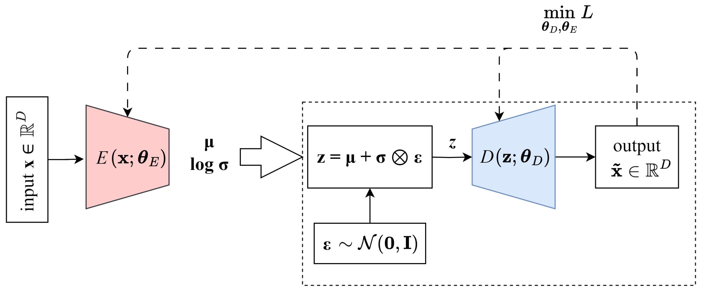
A VAE is a generative model designed to learn a lower-dimensional latent representation of data, enabling controlled and diverse sample generation. Unlike standard autoencoders, which deterministically encode and decode input data, VAEs model the latent space as a probability distribution rather than a fixed set of feature vectors [18]. The VAE consists of an encoder that maps high-dimensional inputs $\mathbf{x}\in {\mathbb{R}}^D$ onto a low-dimensional latent space $\mathbf{z}\in {\mathbb{R}}^d$, $d\ll D$ and a decoder that maps the latent space representations back into the original space, generating an approximate example $\tilde{\mathbf{x}}\in {\mathbb{R}}^D$; see Figure 4.

The encoder predicts the mean $\mathit{\mu }$ and variance ${\mathit{\sigma }}^2$ of the sampled latent representation $\mathbf{z}$. It learns to approximate the posterior distribution $q_{{\mathit{\theta }}_E}\left(\mathbf{z}\right|\mathbf{x})$, ensuring that the latent variables retain a meaningful structure. The decoder, parameterized by ${\mathit{\theta }}_D$, reconstructs an estimate $\tilde{\mathbf{x}}$ of the measured input $\mathbf{x}$ from the sampled latent variable by modeling the likelihood function $p_{{\mathit{\theta }}_D}\left(\tilde{\mathbf{x}}\right|\mathbf{z})$. This probabilistic formulation ensures that the learned latent space remains continuous and structured, allowing for smooth data interpolation and the synthesis of diverse yet coherent maneuvers. The VAE optimizes two key objectives: minimizing the reconstruction loss to ensure accurate data reconstruction and enforcing a prior distribution on the latent space, defined as $p_z\left(\mathbf{z}\right)=\mathcal{N}(\mathit{\mu },diag\left({\mathit{\sigma }}^2\right))$. The reconstruction loss is given by

$$MSE={\displaystyle \frac{1}{N_s}}\sum _{i=1}^{N_s}{\parallel {\tilde{\mathbf{x}}}_i-{\mathbf{x}}_i\parallel }^2.$$

(3)

To enforce the prior, VAE minimizes the Kullback–Leibler (KL) divergence between the approximate posterior $q\left(\mathbf{z}\right|\mathbf{x})$ and the prior $p_z\left(\mathbf{z}\right)$, leading to the total loss [19]

$$L=MSE+D_{\mathrm{KL}}(q\left(\mathbf{z}\right|\mathbf{x})\Vert p_z(\mathbf{z}\left)\right).$$

(4)

In practice, balancing reconstruction accuracy and latent space regularization is crucial. Standard VAEs weigh these terms equally, but in some cases, the KL divergence term dominates early training, leading to poor reconstructions. To address this, the $\beta$-VAE framework [20] introduces a weighting parameter $\beta$, adjusting the trade-off between reconstruction and regularization, i.e.,

$$L=MSE+\beta D_{\mathrm{KL}}(q\left(\mathbf{z}\right|\mathbf{x})\Vert p_z(\mathbf{z}\left)\right).$$

(5)

A higher $\beta$ encourages better latent space organization at the expense of reconstruction accuracy, while a lower $\beta$ prioritizes reconstruction fidelity. This makes $\beta$ a key hyperparameter when designing VAEs for structured generative modeling.

Here, the VAE follows the architecture discussed in [10], utilizing convolutional layers for both the encoder and decoder to effectively process time-series data; see

Table 1. Network topology of the VAE model using convolutional neural networks.

Layer	Output
(a) Encoder
Input	100 × 3
Conv, ReLU	100 × 25
Conv, ReLU	100 × 50
Conv, ReLU	100 × 100
Flatten	10,000
Dense (2x), ReLU	10
Lambda	10
(b) Decoder
Input	10
Dense, ReLU	1000
Reshape	100 × 100
DeConv, ReLU	100 × 50
DeConv, ReLU	100 × 25
Flatten	2500
Dense	300
Reshape	100 × 3

. The encoder progressively reduces the spatial dimensions of the input (1) and (2) from $D=N_t=100$ through successive convolutional layers to a compact latent representation with $d=10$ ensuring that the model captures the most salient features of the input while avoiding redundancy. The decoder uses transposed convolutions to reconstruct D-dimensional trajectories.

Once the VAE model is trained, it learns the distribution parameters of $\mathbf{z}$, i.e., mean $\mathit{\mu }$ and the natural logarithm of variance ${\mathit{\sigma }}^2$ for each of the 10 latent parameters. It should be noted that $\mathit{\mu }$ and ${\mathit{\sigma }}^2$ are not constants but follow individual probability distributions; see [10]. To generate a new cut-in maneuver, independent samples ${\mathit{\epsilon }}_j\sim \mathcal{N}(\mathbf{0},\mathbf{I})$ are drawn from Gaussian distributions, and ${\mathit{\mu }}_j$ and ${\mathit{\sigma }}_j^2$ are picked randomly from their individual distribution described by Gaussian mixture distributions. These quantities are then combined as Hadamard (element-wise) product ${\mathbf{z}}_j={\mathit{\mu }}_j+{\mathit{\sigma }}_j\odot {\mathit{\epsilon }}_j$, where each latent variable is computed as

$$z_i^{\left(j\right)}={\mu }_i^{\left(j\right)}+{\sigma }_i^{\left(j\right)}{\epsilon }_i^{\left(j\right)},i=1,2,\dots ,10.$$

(6)

The resulting latent vector ${\mathbf{z}}_j=[z_1^{\left(j\right)},z_2^{\left(j\right)},\dots ,z_{10}^{\left(j\right)}]$, is then passed through the decoder to generate a synthetic maneuver trajectory ${\tilde{\mathbf{x}}}_j=D\left({\mathbf{z}}_j\right)$, see framed part in Figure 4. This describes a cut-in trajectory ${\tilde{x}}_k^{\left(j\right)}$, $k=1\dots N_t$. By sampling different ${\mathbf{z}}_j$ vectors, we can generate diverse and realistic maneuver trajectories while preserving the underlying distribution learned during training.

4. Generative Adversarial Networks

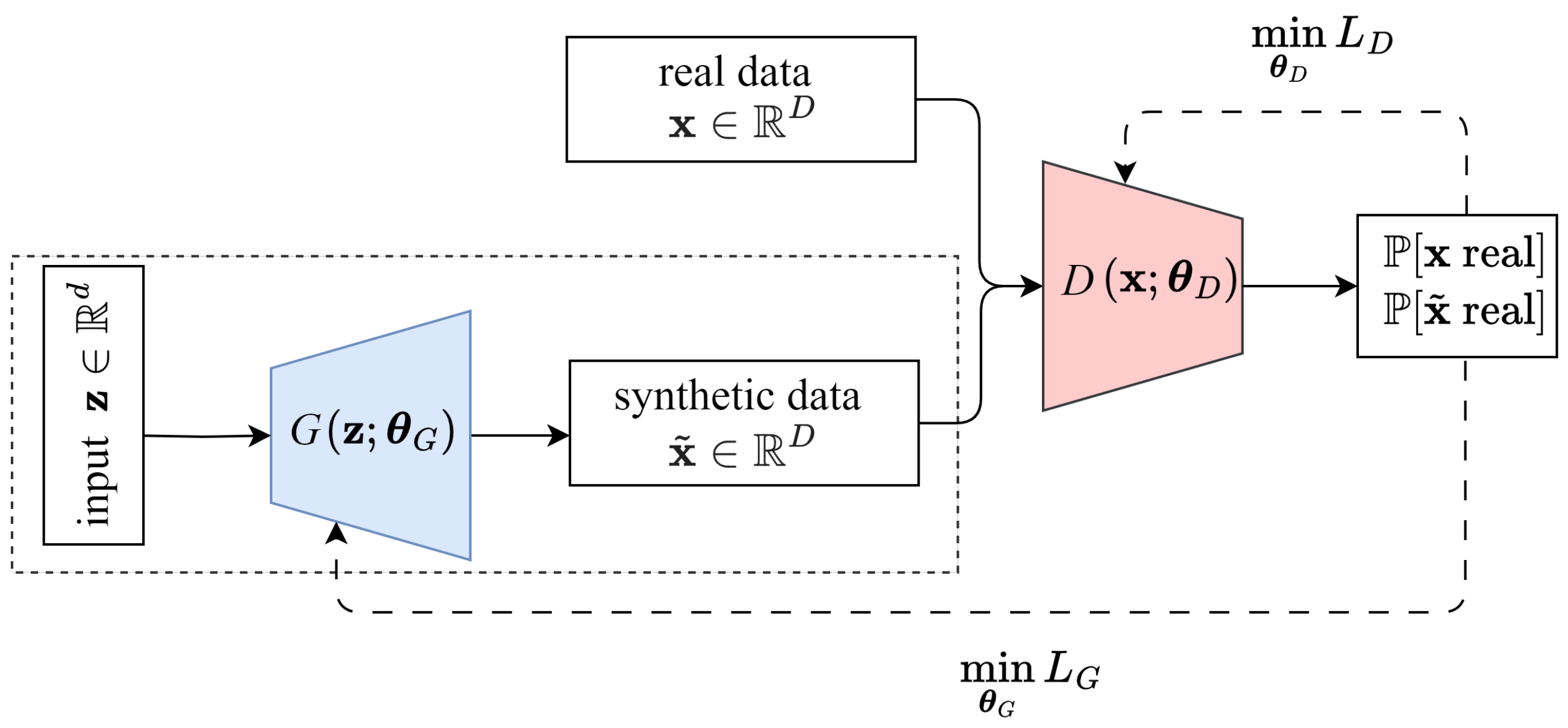
A GAN as shown in Figure 5 consists of two neural networks: a generator (G), similar to the decoder of the VAE, and a discriminator (D), which learns to distinguish between real data and fake data generated by $G\left(z\right)$ from random input. Both are trained in a competitive learning process [15]. The generator aims to synthesize data that closely resemble real samples, while the discriminator classifies samples as real or fake. This competition forces the generator to iteratively refine its outputs until the discriminator can no longer reliably differentiate between them.

In this research, we explore both a basic GAN and a WGAN to evaluate their ability to model the underlying data distribution. The basic GAN provides a standard framework for adversarial training, while the WGAN introduces modifications to improve training stability and reduce mode collapse. The following subsections outline the architectures and training formulations of these models.

4.1. Basic GAN

The basic GAN architecture, illustrated in Figure 5, consists of two neural networks: a generator and a discriminator. The generator transforms a random vector ${\mathbf{z}}_j\in {\mathbb{R}}^d$, sampled from a prior distribution $p_z\left(\mathbf{z}\right)$ typically chosen as a standard Gaussian distribution, into a generated cut-in maneuver ${\tilde{\mathbf{x}}}_j=G\left({\mathbf{z}}_j\right)\in {\mathbb{R}}^D$, where $D=N_t$. Meanwhile, real cut-in maneuvers ${\mathbf{x}}_i$ are selected from the true measured data with the unknown distribution $p_x\left(\mathbf{x}\right)$. The discriminator assigns a probability $D\left(\mathbf{x}\right)\in [0,1]$ to a provided sample, indicating how likely it is to be real. Its objective is to distinguish between real and generated maneuvers, aiming for $D\left({\mathbf{x}}_i\right)\to 1$ for real and $D\left({\tilde{\mathbf{x}}}_j\right)\to 0$ for generated ones [21].

To achieve this, the discriminator maximizes the probability of classifying real trajectories correctly, i.e.,

$$\underset{D}{max}{\mathbb{E}}_{\mathbf{x}\sim p_x\left(\mathbf{x}\right)}\left[logD\left(\mathbf{x}\right)\right].$$

(7)

For generated trajectories $G\left(\mathbf{z}\right)$, it aims to classify them as fake. Due to $\log (1-D)\to 0\mathrm{as}D\to 0$, this is achieved by maximizing the expectation

$$\underset{D}{\max }{\mathbb{E}}_{\mathbf{z}\sim p_z\left(\mathbf{z}\right)}\left[\log (1-D(G\left(\mathbf{z}\right)\left)\right)\right].$$

(8)

Both objectives can be summarized in a common goal for the discriminator:

$$\underset{D}{\max }\left({\mathbb{E}}_{\mathbf{x}\sim p_x\left(\mathbf{x}\right)}\left[\log D\left(\mathbf{x}\right)\right]+{\mathbb{E}}_{\mathbf{z}\sim p_z\left(\mathbf{z}\right)}\left[\log (1-D\left(G\left(\mathbf{z}\right)\right))\right]\right).$$

(9)

Since neural networks are optimized using gradient descent (which minimizes rather than maximizes), the discriminator loss function is usually defined as the negative of objective (9), i.e.,

$$L_D=-{\mathbb{E}}_{\mathbf{x}\sim p_x\left(\mathbf{x}\right)}\left[\log D\left(\mathbf{x}\right)\right]-{\mathbb{E}}_{\mathbf{z}\sim p_z\left(\mathbf{z}\right)}\left[\log (1-D(G\left(\mathbf{z}\right)\left)\right)\right].$$

(10)

In contrast, the generator aims to fool the discriminator by generating trajectories that are classified as real, which may be expressed as

$$\underset{G}{\max }{\mathbb{E}}_{\mathbf{z}\sim p_z\left(\mathbf{z}\right)}\left[\log D\left(G\right(\mathbf{z}\left)\right)\right].$$

(11)

For a minimization algorithm the generator loss function is then

$$L_G=-{\mathbb{E}}_{\mathbf{z}\sim p_z\left(\mathbf{z}\right)}\left[\log D\left(G\right(\mathbf{z}\left)\right)\right].$$

(12)

Both the generator and discriminator are designed using convolutional layers to effectively capture spatial structures in the data, which are in the form of time series in the actual application. The generator employs transposed convolutions to upsample low-dimensional Gaussian noise $\mathbf{z}\in {\mathbb{R}}^d,d=10$, into structured high-dimensional data $\tilde{\mathbf{x}}\in {\mathbb{R}}^D,D=N_t>d$, ensuring realistic feature generation. The discriminator, in contrast, applies standard convolutions to extract hierarchical features, enabling accurate differentiation between real and generated samples. The detailed architectural specifications of the used GAN are summarized in

Table 2. Network topology of the GAN model using convolutional neural networks.

Layer	Output
(a) Generator.
Input	10
Dense, ReLU	800
Reshape	25 × 32
DeConv, ReLU	50 × 64
DeConv, ReLU	100 × 32
Conv, tanh	100 × 3
(b) Discriminator.
Input	100 × 3
Conv, ReLU	50 × 32
Conv, ReLU	25 × 64
Flatten	1600
Dense, ReLU	32
Dense, sigmoid	1

. Maximization ${\max }_D$ and ${\max }_G$ in Equations (9) and (11) refers to training the corresponding convolutional neural network parameters ${\mathit{\theta }}_D$ and ${\mathit{\theta }}_G$.

For generating new cut-in maneuvers, only the framed part in Figure 5 is applied. More specifically, a 10-dimensional random vector ${\mathbf{z}}_j\sim \mathcal{N}(\mathbf{0},\mathbf{I})$ is picked from a standard Gaussian distribution and fed to the generator, resulting in a vector ${\tilde{\mathbf{x}}}_j=G\left({\mathbf{z}}_j\right)$ which represents a synthetic cut-in maneuver according to Equation (1). Throughout the evaluations, we refer to the basic GAN simply as GAN.

4.2. Wasserstein GAN

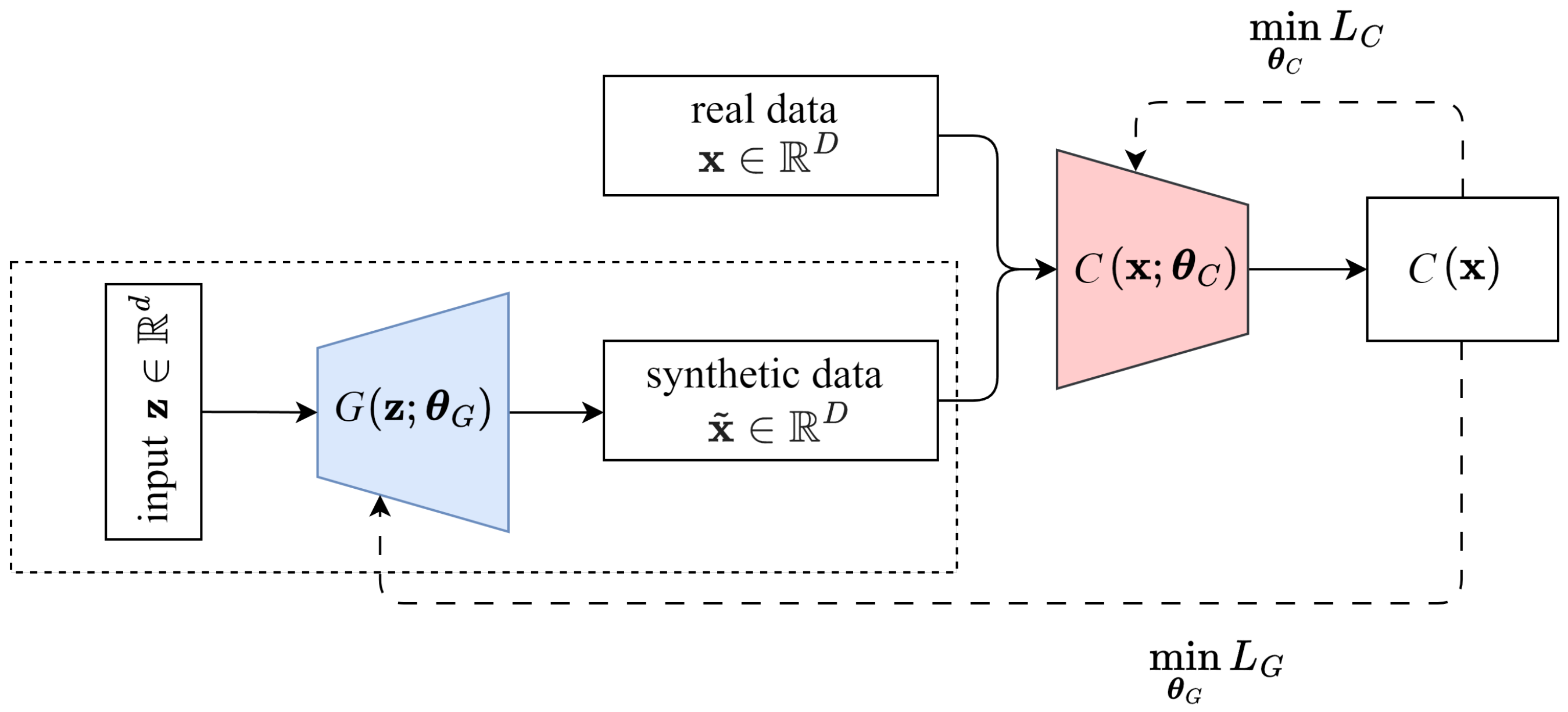
The basic GAN suffers from several challenges, including training instability, mode collapse, and vanishing gradients. These issues arise from the binary classification nature of the discriminator, which can lead to saturated gradients when it becomes too strong, making it difficult for the generator to improve. To improve stability, WGAN modifies the adversarial training framework by replacing the discriminator with a critic that learns to approximate the Wasserstein distance between real and generated distributions [16]; see Figure 6. Unlike a discriminator, which assigns a probability to each trajectory, the critic produces a real-valued score, indicating how real or fake a trajectory is. The Wasserstein distance provides meaningful gradients even when the critic is well trained or when generated trajectories are very poor, which prevents vanishing gradients and mode collapse, resulting in more stable learning dynamics.

The Wasserstein distance between the real data distribution $p_x\left(\mathbf{x}\right)$ and $p_g\left(\tilde{\mathbf{x}}\right)$ of generated trajectories is given by [16]

$$W(p_x,p_g)=\underset{\gamma \in \Gamma (p_x,p_g)}{inf}{\mathbb{E}}_{(\mathbf{x},\tilde{\mathbf{x}})\sim \gamma }\left[\parallel \mathbf{x}-\tilde{\mathbf{x}}\parallel \right],$$

(13)

where $\Gamma (p_x,p_g)$ represents the set of all joint distributions $\gamma (\mathbf{x},\tilde{\mathbf{x}})$ whose marginals are $p_x$ and $p_g$. The inf (infimum) operator finds the lowest possible expected transport cost required to morph one distribution into another. Since solving the above equation directly is intractable, the Kantorovich–Rubinstein duality reformulates the Wasserstein distance into an easier-to-optimize form [22]

$$W(p_x,p_g)=\underset{\parallel f_w{\parallel }_L\le 1}{sup}{\mathbb{E}}_{\mathbf{x}\sim p_x\left(\mathbf{x}\right)}\left[f_w\left(\mathbf{x}\right)\right]-{\mathbb{E}}_{\tilde{\mathbf{x}}\sim p_g\left(\tilde{\mathbf{x}}\right)}\left[f_w\left(\tilde{\mathbf{x}}\right)\right].$$

(14)

Here, sup (supremum) finds the maximum value over all possible 1-Lipschitz functions $f_w$. This allows us to approximate the Wasserstein distance by maximizing the difference in critic scores between real and generated trajectories:

$$\underset{C}{\max }{\mathbb{E}}_{\mathbf{x}\sim p_x\left(\mathbf{x}\right)}\left[f_w\right(\mathbf{x}\left)\right]-{\mathbb{E}}_{\tilde{\mathbf{x}}\sim p_g\left(\tilde{\mathbf{x}}\right)}\left[f_w\right(\tilde{\mathbf{x}}\left)\right],$$

(15)

which ensures that the score for real trajectories remains higher than that for generated ones, guiding the generator to produce more realistic cut-in maneuvers. The Wasserstein metric $f_w$ is generated by the critic $C(\mathbf{x};{\mathit{\theta }}_C)$ to be trained. The maximization is then substituted by the minimization of the loss function

$$L_C=-{\mathbb{E}}_{\mathbf{x}\sim p_x\left(\mathbf{x}\right)}\left[C\right(\mathbf{x}\left)\right]+{\mathbb{E}}_{\tilde{\mathbf{x}}\sim p_g\left(\tilde{\mathbf{x}}\right)}\left[C\right(\tilde{\mathbf{x}}\left)\right].$$

(16)

Originally, the Lipschitz constraint was enforced by clipping weights, which can lead to poor gradient flow and suboptimal performance. To address this, Wasserstein GAN with Gradient Penalty (WGAN-GP) introduces a gradient penalty that better enforces the Lipschitz condition [23]. Instead of weight clipping, the gradient penalty is applied to interpolated points $\widehat{\mathbf{x}}$, which are sampled along straight lines between real and generated data points. This ensures that the critic function maintains a smooth gradient norm close to 1, improving stability and performance. The improved optimization objective is formulated as

$$L_C=-{\mathbb{E}}_{\mathbf{x}\sim p_x\left(\mathbf{x}\right)}\left[C\right(\mathbf{x}\left)\right]+{\mathbb{E}}_{\tilde{\mathbf{x}}\sim p_g\left(\tilde{\mathbf{x}}\right)}\left[C\right(\tilde{\mathbf{x}}\left)\right]+\lambda {\mathbb{E}}_{\widehat{\mathbf{x}}\sim p_{\widehat{x}}\left(\widehat{\mathbf{x}}\right)}{\left(\parallel {\nabla }_{\widehat{\mathbf{x}}}C\left(\widehat{\mathbf{x}}\right){\parallel }_2-1\right)}^2.$$

(17)

The generator aims to produce trajectories that receive higher scores from the critic. This is achieved by maximizing

$$\underset{G}{\max }{\mathbb{E}}_{\tilde{\mathbf{x}}\sim p_g\left(\tilde{\mathbf{x}}\right)}\left[C\right(\tilde{\mathbf{x}}\left)\right]=\underset{G}{\max }{\mathbb{E}}_{\mathbf{z}\sim p_z\left(\mathbf{z}\right)}\left[C\right(G\left(\mathbf{z}\right)\left)\right],$$

(18)

which is reformulated as a minimization problem with the generator loss function

$$L_G=-{\mathbb{E}}_{\mathbf{z}\sim p_z\left(\mathbf{z}\right)}\left[f_w\right(G\left(\mathbf{z}\right)\left)\right].$$

(19)

By leveraging the Wasserstein distance, WGAN already improves training stability compared to basic GAN and reduces mode collapse, while WGAN-GP further enhances convergence and robustness by addressing gradient-related issues. The architecture, detailed in

Table 3. Network topology of the WGAN model using convolutional neural networks.

Layer	Output
(a) Generator.
Input	10
Dense, ReLU	800
Reshape	25 × 32
DeConv, ReLU	50 × 64
DeConv, ReLU	100 × 32
Conv, tanh	100 × 3
(b) Critic.
Input	100 × 3
Conv, LeakyReLU	50 × 64
Conv, LeakyReLU	25 × 128
Flatten	3200
Dense	1

, is the same for both WGAN and WGAN-GP and closely resembles the GAN in Table 2. However, in this work, WGAN-GP is chosen for training, which we will refer to as WGAN for simplicity. Also, the application of the framed generator part in Figure 6 is identical as discussed in Section 4.1.

5. Time-Series Generative Adversarial Network

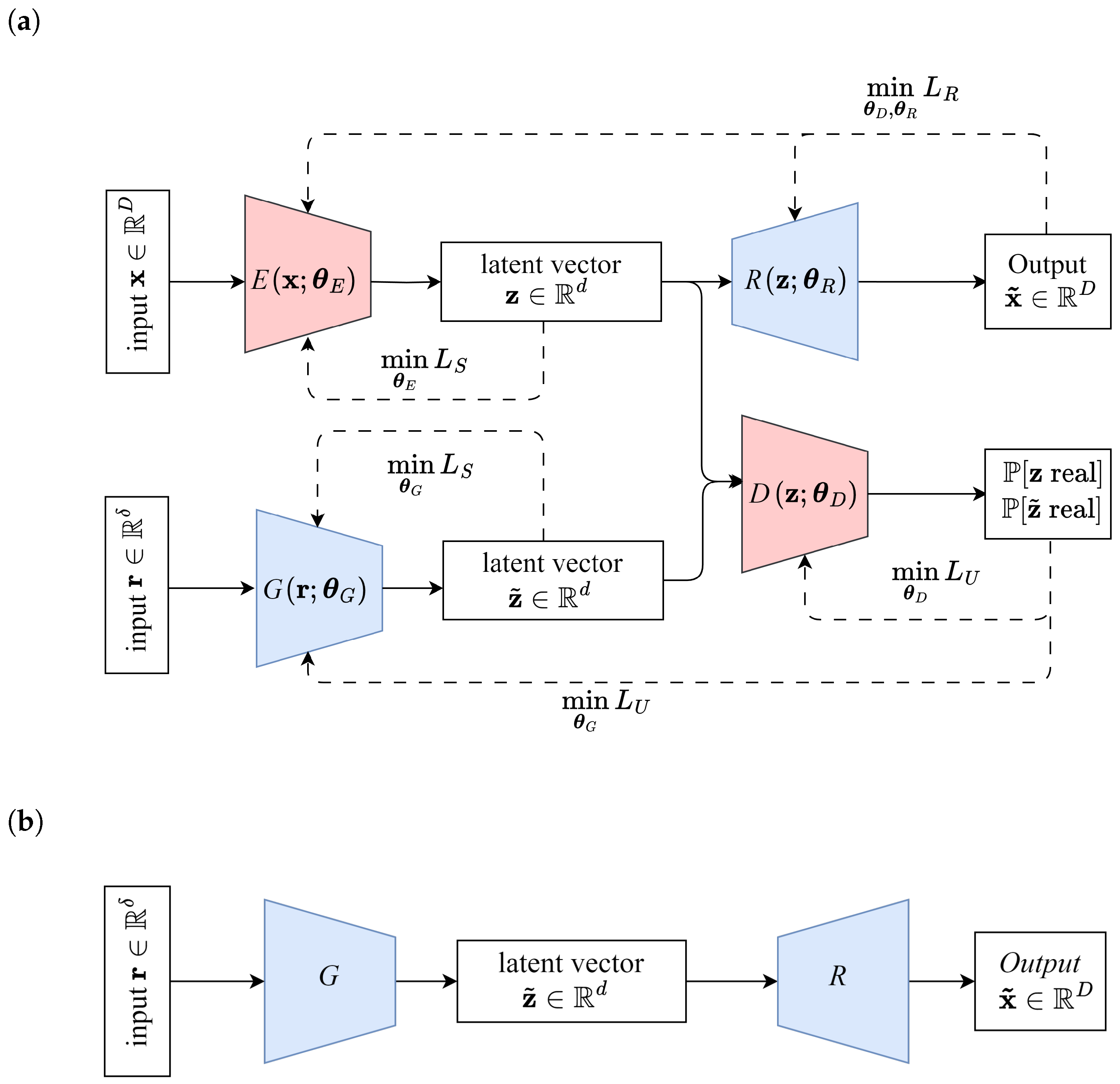
Time-Series Generative Adversarial Network (TimeGAN) is a generative model especially designed for sequential data, integrating both supervised and unsupervised learning to capture complex temporal dependencies [14]. Unlike traditional GANs generating independent samples, TimeGAN explicitly preserves the underlying temporal structure, making it particularly effective and exciting for generating realistic time-series sequences. The model consists of four key components: an embedder E, a recovery network R, a generator G, and a discriminator D. See Figure 7a. The embedder encodes real input trajectories ${\mathbf{x}}_i\in {\mathbb{R}}^D,D=N_t$, into a structured latent representation ${\mathbf{z}}_i=E\left({\mathbf{x}}_i\right)\in {\mathbb{R}}^d$, while the recovery network reconstructs the original trajectories ${\tilde{\mathbf{x}}}_i=R\left({\mathbf{z}}_i\right)\in {\mathbb{R}}^D$ from the latent space to ensure that the temporal relationships are preserved. The generator synthesizes new latent representations ${\tilde{\mathbf{z}}}_j=G\left({\mathbf{r}}_j\right)\in {\mathbb{R}}^d$ from random input ${\mathbf{r}}_j\in {\mathbb{R}}^{\delta }$ taken from a prior distribution ${\mathbf{r}}_j\sim \mathcal{N}(\mathbf{0},\mathbf{I})$ which is chosen as standard Gaussian distribution. The discriminator distinguishes between real and generated latent representations, enforcing realism in the generated latent vectors ${\mathbf{z}}_j$. By combining these components, TimeGAN jointly learns an embedding space for sequential data while simultaneously training a generator and discriminator in an adversarial setting. This hybrid approach allows the model to retain long-term dependencies while ensuring that generated sequences follow realistic temporal patterns.

The training process consists of two phases: embedding learning and adversarial training. In the first phase, the embedder and recovery network are optimized to learn a structured latent representation. Given real measured trajectories $\mathbf{x}\sim p_x\left(\mathbf{x}\right)$, the embedder maps them to latent representations $\mathbf{z}=E\left(\mathbf{x}\right)$, and the recovery network reconstructs the original sequence as $\tilde{\mathbf{x}}=R\left(\mathbf{z}\right)$. Minimization of the reconstruction loss [14]

$$L_R({\mathit{\theta }}_E,{\mathit{\theta }}_R)=\mathbb{E}[\parallel \mathbf{x}-\tilde{\mathbf{x}}{\parallel }^2].$$

(20)

ensures that the recovered sequences closely match the original ones. To enforce temporal structure in the generated latent representations, TimeGAN introduces a supervised loss $L_s$, which aligns the latent space $\mathbf{z}=E\left(\mathbf{x}\right)$ learned by the embedder with the latent space $\tilde{\mathbf{z}}=G\left(\mathbf{r}\right)$ learned by the generator. This is performed by minimizing the loss expectation

$$L_s({\mathit{\theta }}_E,{\mathit{\theta }}_G)=\mathbb{E}[\parallel \mathbf{z}-\tilde{\mathbf{z}}{\parallel }^2].$$

(21)

Both losses are combined and minimized together with respect to the embedder, recovery, and generator network parameters:

$$\underset{{\mathit{\theta }}_E,{\mathit{\theta }}_R,{\mathit{\theta }}_G}{min}(\lambda L_s+L_r),$$

(22)

where $\lambda$ is a hyperparameter that controls the balance between supervised and reconstruction loss. This step ensures that the latent space remains structured, facilitating stable adversarial training.

In the second phase, adversarial training is applied to improve the quality of generated trajectories. The discriminator attempts to classify whether a given latent representation is real $\mathbf{z}$ or generated $\tilde{\mathbf{z}}$. The adversarial loss for improving the discriminator is defined similar to Equation (10), however, with the latent vector $\mathbf{z}$ as input:

$$L_u({\mathit{\theta }}_D,{\mathit{\theta }}_G)=-\mathbb{E}\left[\log D\left(\mathbf{z}\right)\right]-\mathbb{E}\left[\log (1-D\left(\tilde{\mathbf{z}}\right))\right],$$

(23)

where $\mathbf{z}=E\left(\mathbf{x}\right)$ represents the real latent representation, and $\tilde{\mathbf{z}}=G\left(\mathbf{r}\right)$ represents the generated latent representation. The generator G is trained to minimize a combination of the supervised loss (21) and the adversarial loss (23), i.e.,

$$\underset{{\mathit{\theta }}_G}{min}(\eta L_s+L_u),$$

(24)

where $\eta$ is a hyperparameter that controls the trade-off between supervised learning and adversarial learning. Meanwhile, the discriminator D is trained to maximize the adversarial loss (23) with respect to discriminator parameters ${\mathit{\theta }}_D$, i.e.,

$$\underset{{\mathit{\theta }}_D}{\max }{L}_u.$$

(25)

Unlike traditional GANs that rely purely on adversarial feedback, TimeGAN explicitly aligns the latent representations learned from real and generated data through $L_s$. This ensures that the generator produces meaningful latent sequences rather than simply fooling the discriminator. The hyperparameters $\lambda$ and $\eta$ in Equations (22) and (24) control the trade-offs between supervised, reconstruction, and adversarial components but are generally robust in practice. Typically, they are set to $\lambda =1$ and $\eta =10$, also used here.

TimeGAN was originally implemented with Recurrent Neural Network (RNN) layers. However, here it is adapted to convolutional neural network-based architectures for consistency with the other models. The detailed structure of the generator, discriminator, embedder, and reconstructor networks is given in

Table 4. Network topology of the TimeGAN model using convolutional neural networks.

Layer	Output
(a) Generator.
Input	50
Dense, ReLU	800
Reshape	25 × 32
DeConv, ReLU	50 × 64
DeConv, ReLU	100 × 32
Conv, tanh	100 × 10
(b) Discriminator.
Input	100 × 10
Conv, ReLU	50 × 32
Conv, ReLU	25 × 64
Flatten	1600
Dense, ReLU	32
Dense, sigmoid	1
(c) Embedder.
Input	100 × 3
Conv, ReLU	100 × 100
Conv, ReLU	100 × 50
Conv, ReLU	100 × 25
Dense, ReLU	100 × 10
(d) Reconstructor.
Input	100 × 10
Dense, ReLU	100 × 25
DeConv, ReLU	100 × 50
DeConv, ReLU	100 × 100
DeConv, ReLU	100 × 200
Dense, tanh	100 × 3

. For generating new cut-in maneuvers, random vectors ${\mathbf{r}}_j\in {\mathbb{R}}^{\delta },\delta =50$ are picked from a standard Gaussian distribution, transformed into the latent space by the generator G, and finally transformed into synthetic maneuvers ${\tilde{\mathbf{x}}}_j$ by the recovery network R; see Figure 7b.

6. Parameter Training and Computation Time

All models are trained on a workstation with a 6-core CPU and a Quadro T2000 GPU (8GB VRAM). Training configurations are adjusted based on model complexity and convergence behavior to ensure stable learning. Due to their adversarial nature, GAN-based models require more training epochs than VAE. Therefore, the total training duration varies across the models. VAE is trained for 1000 epochs, while GAN and WGAN require 1500 epochs to achieve stable loss values. Due to its higher iteration requirements, TimeGAN is trained for 2000 epochs. To prevent overfitting, early stopping is applied, halting training once validation loss plateaus.

Hyperparameters, including batch size, learning rate, and optimizer, are tuned using grid search across all models. Additionally, model-specific parameters are optimized: the update ratio and gradient penalty weight ($\lambda$) for WGAN, and the KL divergence loss weight for VAE. A batch size of 32 is used for all models. ADAM optimization is applied to VAE with a learning rate of 0.00001 (${\beta }_1=\mathrm{default}, {\beta }_2=\mathrm{default}$) and a KL divergence loss weight of 0.001, GAN with a learning rate of 0.0002 (${\beta }_1=0.5, {\beta }_2=\mathrm{default}$), and TimeGAN with a learning rate of 0.0001 (${\beta }_1=\mathrm{default}, {\beta }_2=\mathrm{default}$). RMSprop is used for WGAN with a learning rate of 0.00005 to improve stability. For WGAN, we use a generator-to-critic training ratio of 1:3 and apply a gradient penalty with $\lambda =10$ to enforce the Lipschitz constraint.

As shown in

Table 5. Comparison of model training time and inference efficiency.

Model	Training Time	Inference Time
VAE	10m (500 epochs)	11.54 ms
GAN	2 h 48 m (1500 epochs)	4.64 ms
WGAN	2 h 55 m (1500 epochs)	4.48 ms
TimeGAN	19 h 45 m (2000 epochs)	129 ms

, VAE has the shortest training time, completing its 500 epochs significantly faster than the other models. However, its inference time is more than twice that of GAN-based models. In contrast, GAN and WGAN require much longer training durations, taking approximately 17 times longer than VAE, but achieve inference speeds over 60% faster. TimeGAN is the least efficient model, with a training time over six times longer than GAN and WGAN and an inference time more than eleven times that of VAE.

7. Qualitative Analysis of Generated Cut-In Maneuvers

A qualitative evaluation may be performed by using heatmaps, t-Distributed Stochastic Neighbor Embedding (t-SNE), or kernel density estimation (KDE). The goal is to gain insight into the data distribution and the model’s ability to capture underlying patterns. Heatmaps are used to examine structural similarities, capture spatial and temporal variations, and to highlight alignment and divergence between synthetic and real maneuvers. t-SNE is a nonlinear dimension reduction technique that maps high-dimensional data into a lower-dimensional space, typically two or three dimensions, while preserving neighborhood relationships. This mapping enables the representation of the $N_t$-dimensional data ${\mathbf{d}}_i$ and ${\mathbf{v}}_i$ in 2D, allowing for a visual assessment of how well the generated samples resemble real data. To complement these visual analyses, KDE plots provide a statistical comparison of data distributions. KDE estimates the probability density function of a dataset, offering a smooth representation that helps to evaluate how closely generated samples match the statistical properties of the real dataset. By jointly analyzing heatmaps, t-SNE plots, and KDE plots, we obtain a comprehensive qualitative and statistical evaluation of the generated data, and thus a first assessment of the underlying generative models.

7.1. Heatmaps

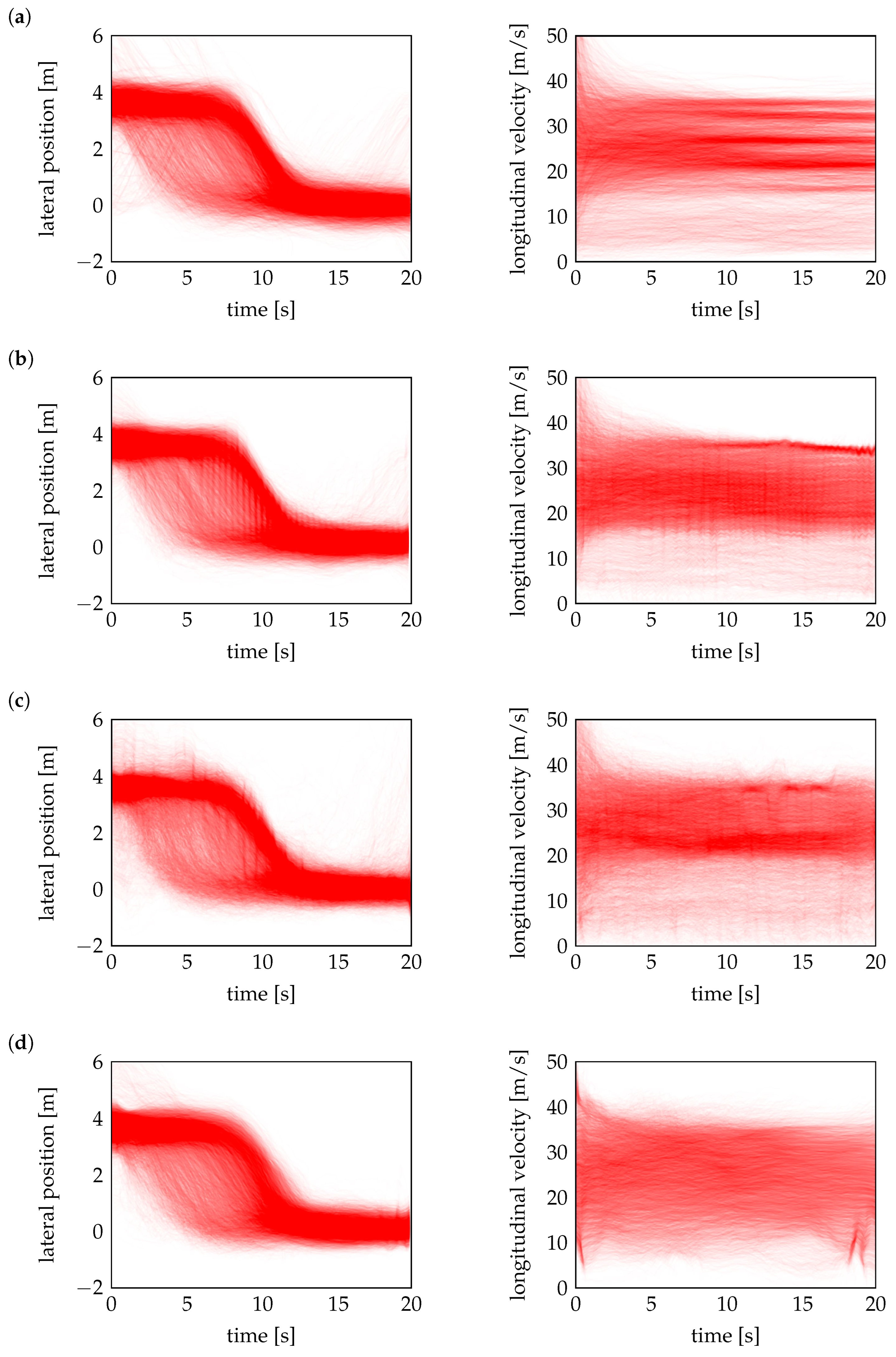
The full dataset of over 8000 measured trajectories for lateral position ${\mathbf{d}}_i$ and longitudinal velocity ${\mathbf{v}}_i$ is visualized in Figure 2, while their equal number of generated counterparts denoted as ${\tilde{\mathbf{d}}}_i$ and ${\tilde{\mathbf{v}}}_i$ are shown in Figure 8. A visual comparison of heatmaps already allows to clearly assess how well the models preserve the underlying temporal structure and dynamics.

Among the evaluated models, VAE demonstrates the best performance, generating trajectories that closely align with the measured data. As shown in Figure 8a, its trajectories exhibit smooth transitions and accurately capture underlying patterns, ensuring high trajectory realism. The basic GAN in Figure 8b performs reasonably well, producing less noisy outputs compared to the other GAN-based models in Figure 8c,d. However, its trajectories remain less smooth and structured than those of VAE, particularly in velocity. The WGAN exhibits the greatest irregularity with high noise level, reducing the overall trajectory realism. TimeGAN also generates noisy trajectories but performs slightly better than WGAN. Due to the noisy trajectories, all three models except the VAE require post-processing to ensure stability before being used in simulation testing, whereas the trajectories generated by the VAE are sufficiently smooth for direct use. The noise also makes it difficult to clearly distinguish different probabilistic modes through direct trajectory observation, necessitating deeper analysis using techniques such as t-SNE and kernel density estimation (KDE) to properly assess the diversity and structural coverage of the generated scenarios.

7.2. Distributed Stochastic Neighbor Embedding

To assess the similarity between different trajectories, we compare their distances in a structured manner. By introducing the feature vector (2), each cut-in trajectory is represented as a point in the $N_t$-dimensional feature space, where its relative distance

$${\Delta }_{ij}=\parallel {\mathbf{x}}_i-{\mathbf{x}}_j\parallel =\sqrt{\sum _{k=1}^{N_t}{(x_k^{\left(i\right)}-x_k^{\left(j\right)})}^2},i,j=1\dots N_S,$$

(26)

to other trajectories ${\mathbf{x}}_j$ provides insight into its similarity. If two points ${\mathbf{x}}_i$ and ${\mathbf{x}}_j$ are close in the feature space, their associated maneuvers $x_k^{\left(i\right)}$ and $x_k^{\left(j\right)}$ exhibit similar movement patterns. However, the direct visualization of these neighborhood relationships in the high-dimensional space is not feasible (as here $N_t$ = 100), making it necessary to map the data into a two-dimensional representation while preserving neighborhood structures.

Such a mapping can be achieved by using t-SNE [24], which is an improved version of SNE [25]. While SNE is assuming Gaussian distribution in both spaces, i.e, the original $\mathbf{x}$-space and the mapped $\mathbf{y}$-space, t-SNE assumes a t-distribution in the $\mathbf{y}$-space. The transformation

$$\gamma :{\mathbb{R}}^{N_t}\to {\mathbb{R}}^2,\mathbf{y}=\gamma \left(\mathbf{x}\right),$$

(27)

is applied independently to real and generated datasets, mapping their high-dimensional representations into a two-dimensional space, which then allows to visualize trajectory distributions for each dataset separately and compare their overall patterns.

The t-SNE computes a probability distribution of the distances (26) using a Gaussian kernel:

$$p_{ij}={\displaystyle \frac{exp(-{\Delta }_{ij}^2/2{\sigma }_i^2)}{{\sum }_{k\ne i}exp(-{\Delta }_{ik}^2/2{\sigma }_i^2)}},$$

(28)

where higher values of $p_{ij}$ indicate stronger similarity between trajectories ${\mathbf{x}}_i$ and ${\mathbf{x}}_j$. The variance ${\sigma }_i^2$ is determined individually for each point, adapting to local density variations. Acting as a bandwidth parameter for the Gaussian kernel, it dynamically scales distances to control how local or global the similarity assessment is. In dense regions, a smaller ${\sigma }_i$ focuses on immediate neighbors, while in sparse regions, a larger ${\sigma }_i$ broadens the influence to distant points. The value of ${\sigma }_i$ is adjusted such that the effective number of neighbors each point considers remains approximately constant.

In the two-dimensional visualization space, the same concept is applied, but instead of a Gaussian kernel, a Student’s t-distribution with one degree of freedom is used, which is equivalent to a Cauchy distribution and provides better results:

$$q_{ij}={\displaystyle \frac{{(1+{\delta }_{ij}^2)}^{-1}}{{\sum }_{k\ne i}{(1+{\delta }_{ik}^2)}^{-1}}},$$

(29)

where ${\delta }_{ij}=\parallel {\mathbf{y}}_i-{\mathbf{y}}_j\parallel$ represents the Euclidean distance in the two-dimensional $\mathbf{y}$-space. Due to normalization, both quantities $p_{ij}$ and $q_{ij}$ can be interpreted as observations of associated probability distributions P and Q in both spaces. The two point clouds ${\mathbf{x}}_i$ and ${\mathbf{y}}_i$ have the same neighbor characteristics if their corresponding distributions (28) and (29) are identical. A possible measure of the similarity of the two probability distributions is the Kullback–Leibler (KL) divergence defined as

$$C=D_{\mathrm{KL}}\left(P\right|\left|Q\right)=\sum p_{ij}\log {\displaystyle \frac{p_{ij}}{q_{ij}}}.$$

(30)

Similarity is enforced by moving the mapped points ${\mathbf{y}}_i$ such that C is minimized where a gradient search with a momentum term is used as the training procedure to finally obtain the mapping (27).

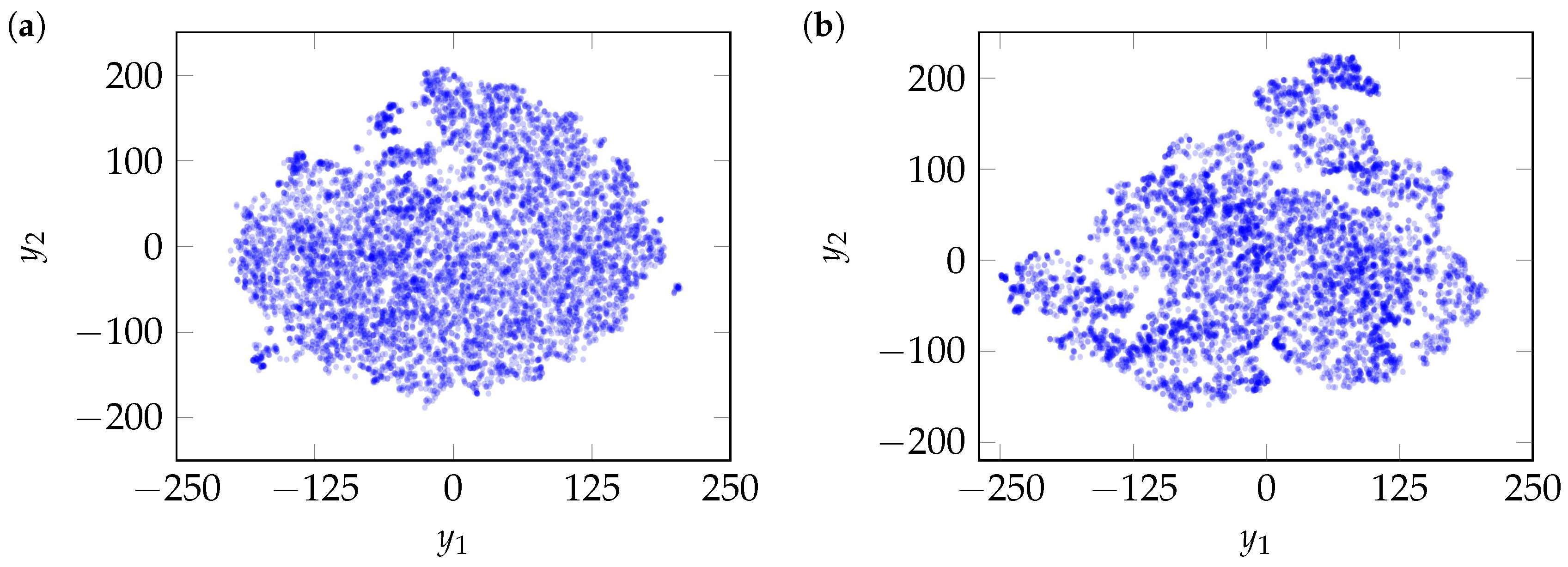
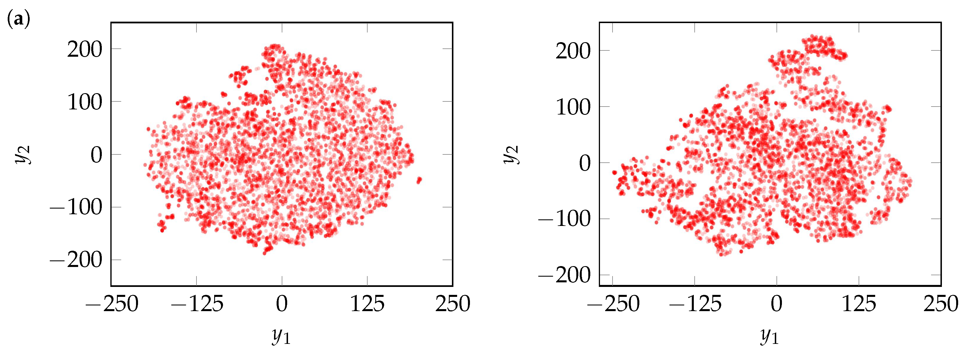
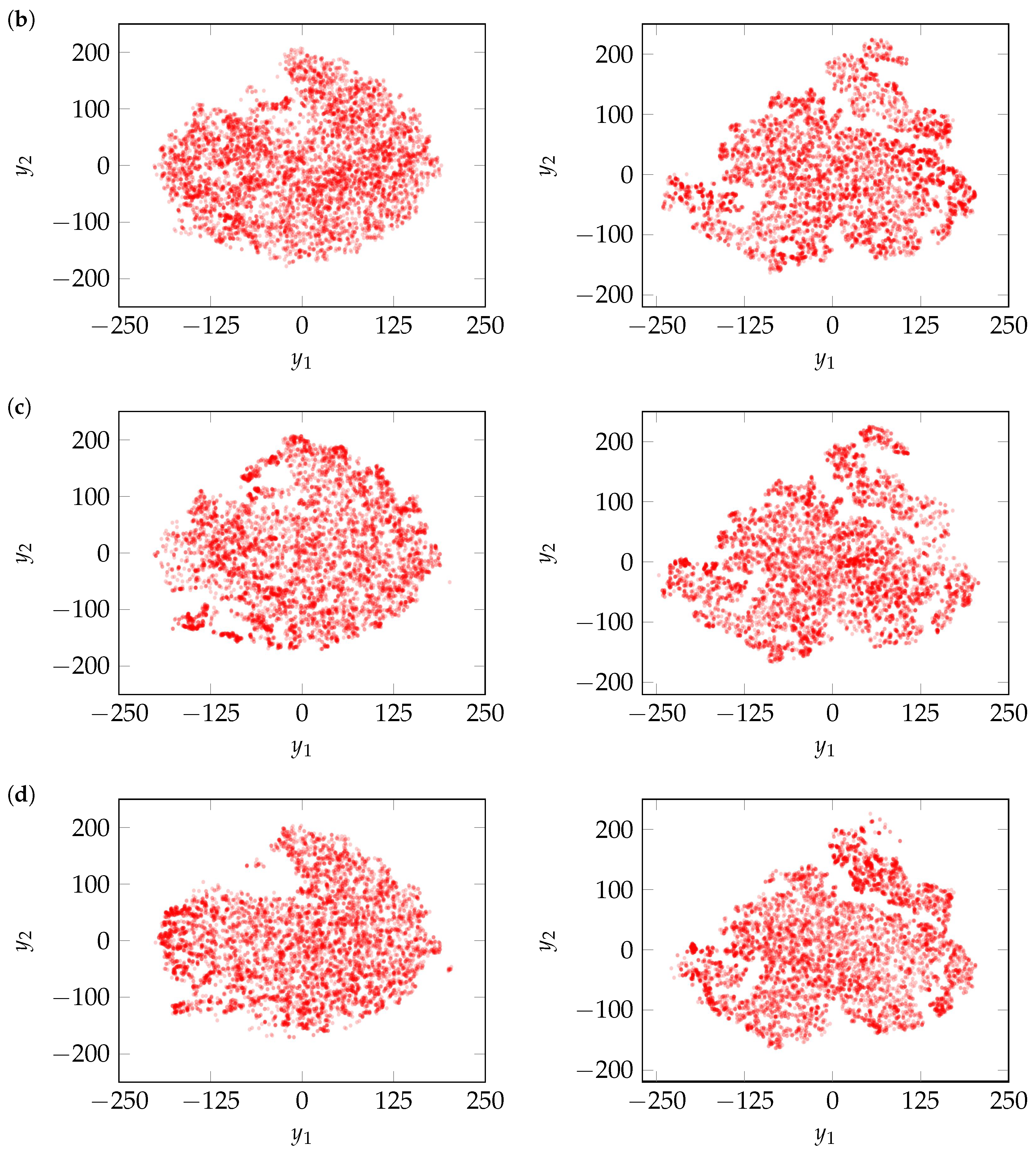
The application of t-SNE to the measured maneuvers (2) results in the point clouds ${\mathbf{y}}_i$ illustrated in Figure 9. Similarly, t-SNE is applied separately to the generated maneuvers ${\tilde{\mathbf{x}}}_i$ in Figure 8 yielding the point clouds ${\tilde{\mathbf{y}}}_i$ shown in Figure 10. By comparing them with Figure 9, the performance of the generative models may be assessed. If the generated clustering patterns align closely with those of the measured data in the two-dimensional space, this indicates that the model has successfully captured the underlying structure of the measured cut-in maneuvers.

VAE and WGAN demonstrate comparable performance, effectively covering the entire mapped measured data space and preserving the cluster structure as shown in Figure 10a,c. The former suggests a strong capture of diversity, while the latter indicates similarity in maneuver distributions. GAN and TimeGAN also perform well. However, both models miss certain regions and show minor inconsistencies in clustering. Even though these models exhibit less noise in the heatmap comparison (compared to WGAN), their reduced diversity becomes evident when analyzed with t-SNE. The improved coverage of WGAN is attributed to its use of the Wasserstein loss, which encourages alignment with the full data distribution and mitigates mode collapse despite noisier trajectory outputs. TimeGAN, in particular, exhibits more pronounced mode issues, identified through missing regions, uneven cluster densities, and the over-concentration of trajectories, likely due to its latent space training strategy that simplifies the learning task but increases the risk of overfitting to dominant patterns and reduces overall diversity.

7.3. Statistical Analysis Using KDE

While heatmaps and t-SNE plots reveal structural similarities between real and generated data, kernel density estimation [26,27] provides a statistical perspective on distribution alignment. The conformity of probability distributions is essential to obtain a correct risk assessment from the simulation of generated cut-in scenarios [10].

KDE is applied to the data ${\mathbf{x}}_i$ and ${\tilde{\mathbf{x}}}_i$ in the $\mathbf{x}$-space to compute smooth estimates of probability density functions by superposing Gaussian kernel densities. Given a set of observations $x_1,x_2,\dots ,x_n$, the estimated density at any value x of a random variable X is approximately

$$f_x\left(x\right)\approx {\displaystyle \frac{1}{nh}}\sum _{l=1}^{n}K\left({\displaystyle \frac{x-x_l}{h}}\right),$$

(31)

where $K\left(x\right)$ is a kernel function (typically Gaussian, i.e., $K\left(x\right)=exp(-x^2/2)/\sqrt{2\pi }$), h is the bandwidth parameter controlling smoothness, and n is the number of samples [26]. This non-parametric method ensures a smooth approximation of the data distribution without assuming any predefined shape. To facilitate better comparability, KDE is applied separately to ${\mathbf{d}}_i$ and ${\mathbf{v}}_i$, disregarding the potential correlation effects, where the measurements ${\mathbf{x}}_k^{\left(i\right)}$ of all time points $t_k$ and the total set of cut-in maneuvers are summarized in a singe dataset, i.e., $x_l\in \{d_k^{\left(i\right)},i=1,\dots ,N_S,k=1,\dots ,N_t\}$ or $x_l\in \{v_k^{\left(i\right)},i=1,\dots ,N_S,k=1,\dots ,N_t\}$, resulting in $n=N_s{N}_t$.

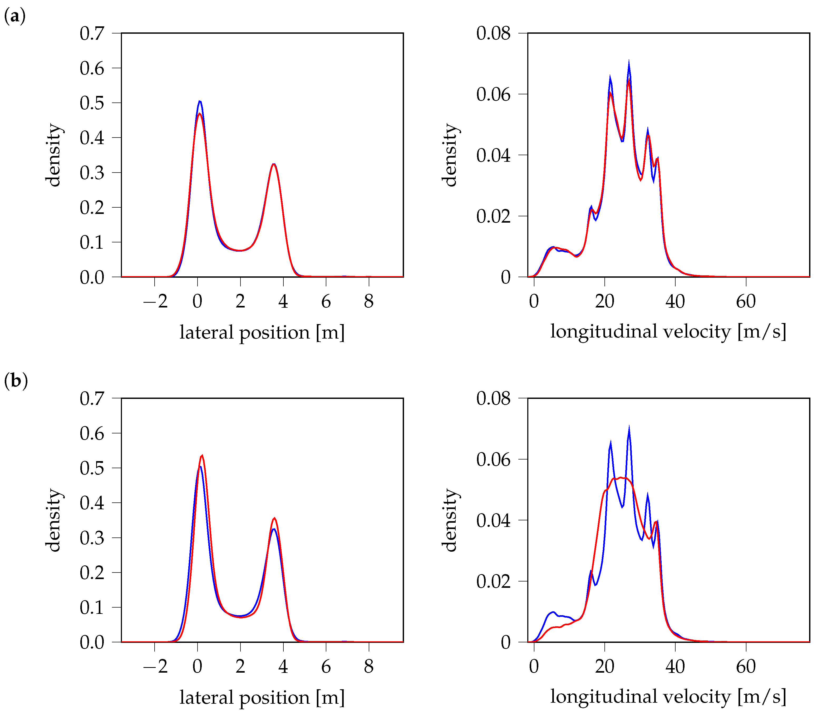
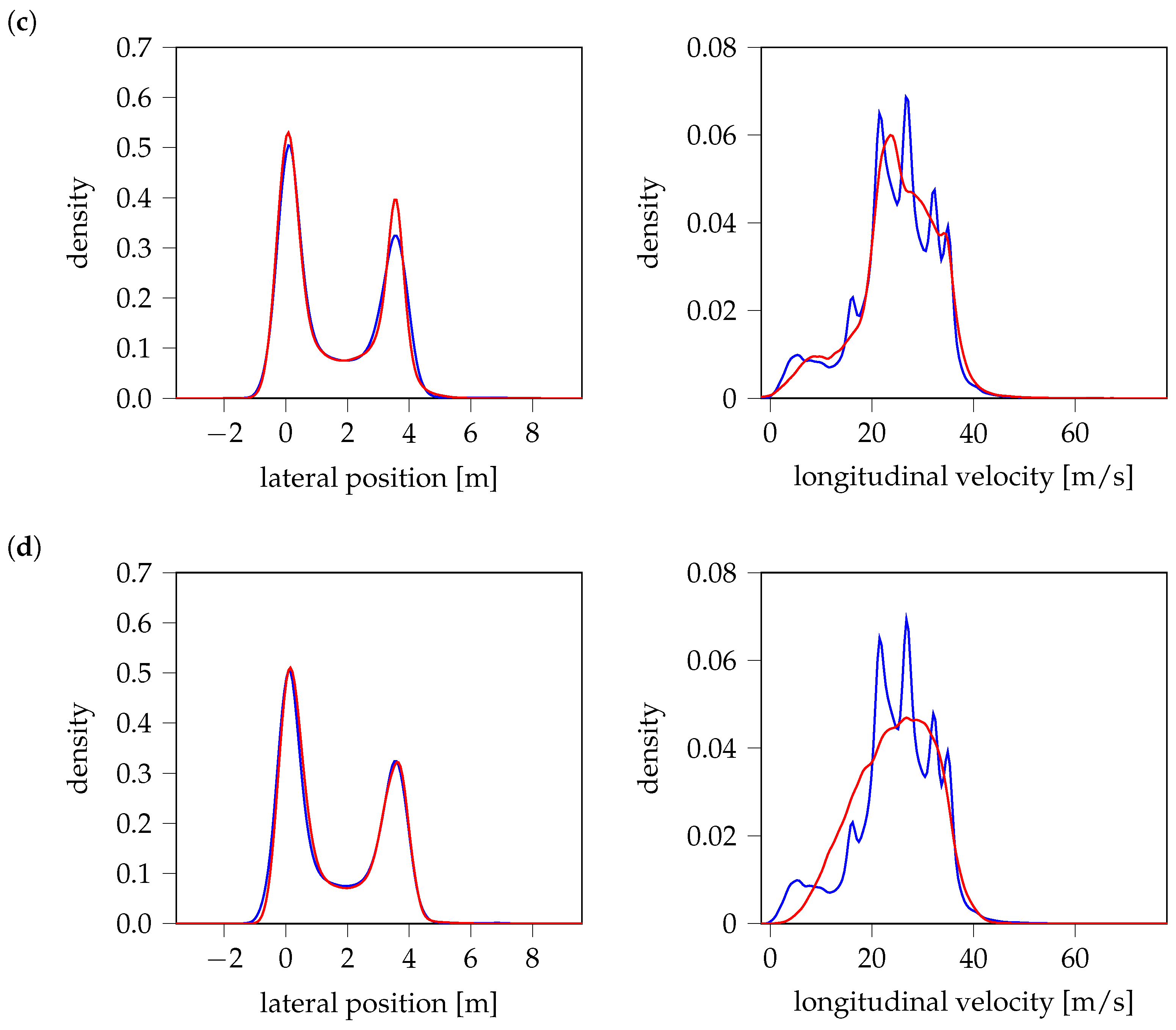
Figure 11 presents KDE comparisons across models, where blue curves represent the probability density of measured data, and red curves correspond to generated data, respectively. All models closely match the distributions in the lateral position. However, discrepancies emerge in the longitudinal velocity, where VAE performs best, capturing the full distribution. WGAN follows, though it fails to represent all modes, leading to partial coverage only. In contrast, both TimeGAN and GAN struggle significantly, failing to recover key modes of the velocity distribution. It should be noted that variations in peak probabilities highlight associated cut-in maneuvers with a significantly higher or lower proportion of such cases in the generated test scenarios compared to real-world driving data. Consequently, this leads to an over- or underestimation of the failure probability of Advanced Driver Assistance Systems (ADASs) [10], depending on how critical these maneuvers are.

8. Quantitative Metrics for the Comparison of Generated Results

Quantitative metrics are an essential complement for evaluating model performance, especially when visual methods such as t-SNE plots or KDE analyses suggest closely aligned results. While our qualitative evaluation highlights distinct variations across different aspects, such as noise and diversity, quantitative metrics help to unify these insights, providing a more comprehensive and objective assessment of realism and overall data representation. To assess the models quantitatively, two primary metrics are utilized: Mean of Incoming Variance of Outgoing (MiVo) [28] and the Hungarian distance [7].

Given the large dataset size of more than 8000 trajectories, the computational efficiency of these metrics is optimized by replacing Dynamic Time Warping (DTW) with Euclidean distance as the trajectory similarity measure. This adaptation is validated through mixing and discriminability tests [28] to ensure that the modified metrics remains reliable and robust. Additionally, a 1:1 ratio of real to generated samples is maintained across all evaluations to enable balanced comparisons. A sample efficiency test [28] reveals that the 1:1 ratio is optimal, and even when the proportion of generated samples is increased, the metrics remains consistent, indicating that higher ratios do not significantly impact reliability.

8.1. Mean of Incoming Variance of Outgoing (MiVo)

Similar to (26), MiVo [28] measures the differences in between generated and real trajectories, i.e.,

$${\Delta }_{ji}=\parallel {\tilde{\mathbf{x}}}_j-{\mathbf{x}}_i\parallel =\sqrt{\sum _{k=1}^{N_t}{\left({\tilde{x}}_k^{\left(j\right)}-x_k^{\left(i\right)}\right)}^2},i,j=1,\dots ,N_s.$$

(32)

If for example ${\Delta }_{ji}=0$, this means that there exists a generated counterpart ${\tilde{\mathbf{x}}}_j$ that is identical to a measured maneuver ${\mathbf{x}}_i$. By comparing each measured maneuver ${\mathbf{x}}_i$ (outgoing) with all generated maneuvers ${\tilde{\mathbf{x}}}_j$ (incoming), we obtain $N_s^2$ distances, summarized in a distance matrix

$$\Delta =\left(\begin{array}{cccc}{\Delta }_{11}& {\Delta }_{12}& \dots & {\Delta }_{1,N_s}\\ {\Delta }_{21}& {\Delta }_{22}& \dots & {\Delta }_{2,N_s}\\ ⋮& ⋮& \ddots & ⋮\\ {\Delta }_{N_s,1}& {\Delta }_{N_s,2}& \dots & {\Delta }_{N_s,N_s}\end{array}\right).$$

(33)

In order to find the most similar real maneuver ${\mathbf{x}}_i$ to a specific generated maneuver ${\tilde{\mathbf{x}}}_j$, we minimize the elements of the distance matrix along its j-th row, i.e.,

$$i=arg\underset{k}{min}{\Delta }_{jk}.$$

(34)

Performing this for all ${\tilde{\mathbf{x}}}_j$ results in an incoming distance vector of nearest neighbors

$$\mathit{\delta }={\left[\underset{k}{min}{\Delta }_{1,k},\underset{k}{min}{\Delta }_{2,k},\dots ,\underset{k}{min}{\Delta }_{N_s,k}\right]}^{\top }.$$

(35)

The values ${\delta }_j$ in vector $\mathit{\delta }$ represent the distances to the closest real counterpart ${\mathbf{x}}_i$ for each generated maneuver ${\tilde{\mathbf{x}}}_j$, respectively. Lower values suggest that generated maneuvers are highly realistic, meaning they closely resemble real-world maneuvers. Since realism should be evaluated based on the overall proximity of generated data to real data, the mean of $\mathit{\delta }$ is taken. A low mean value indicates that, on average, generated samples are well aligned with real data.

Similarly, to find the most similar generated maneuver ${\tilde{\mathbf{x}}}_j$ to a specific real maneuver ${\mathbf{x}}_i$, the elements of the distance matrix may be minimized along its i-th column, i.e.,

$$j=arg\underset{k}{min}{\Delta }_{ki}.$$

(36)

Performing this for all ${\mathbf{x}}_i$ results in an outgoing distance vector of nearest neighbors

$$\tilde{\mathit{\delta }}={\left[\underset{k}{min}{\Delta }_{k,1},\underset{k}{min}{\Delta }_{k,2},\dots ,\underset{k}{min}{\Delta }_{k,N_s}\right]}^{\top }.$$

(37)

The values ${\tilde{\delta }}_i$ in vector $\tilde{\mathit{\delta }}$ indicate how well the generated data points ${\tilde{\mathbf{x}}}_j$ cover the real data ${\mathbf{x}}_i$. If all real maneuvers have close generated counterparts, this means that the generative model provides diverse and well-distributed outputs. However, if some real maneuvers have very close generated matches while others are not covered by close counterparts, this suggests an uneven distribution of generated samples. To capture this variation, the variance of $\tilde{\mathit{\delta }}$ is taken, which quantifies how consistently the real maneuvers are matched by generated ones. A low variance indicates that generated data points are evenly distributed across the real dataset, avoiding cases where certain real maneuvers are well represented, while others are ignored. Both quantities may be summarized in a metric

$$\rho =mean\left(\mathit{\delta }\right)+variance\left(\tilde{\mathit{\delta }}\right),$$

(38)

where a low value indicates a well-performing generative model producing synthetic maneuvers with high realism capturing the full variety of potential cut-in maneuvers. An example in the Appendix A demonstrates the computation of these quantities.

The application of MiVo to the synthetic maneuvers in Figure 8 yields the values presented in the second column of

Table 6. Comparison of generative AI models with the VAE model.

Model	MiVo	Hungarian Distance	Difference to VAE
			MiVo	Hungarian
VAE	0.155297	0.246246	−	−
GAN	0.252633	0.325716	+62.68%	+32.27%
WGAN	0.253929	0.298249	+63.51%	+21.12%
TimeGAN	0.265483	0.344059	+70.95%	+39.72%

. As expected, VAE performs the best, with a noticeable gap to the other GAN-based models, which show relatively similar values. Among them, TimeGAN has the highest MiVo value, likely due to its limited diversity as already seen in the t-SNE and KDE plots, where it misses certain regions. While MiVo effectively identifies major differences, it is less sensitive to minor differences, such as those between GAN and WGAN, where global structure improvements are offset by increased local noise. This limitation highlights the need for a more precise evaluation, which is why we also apply the Hungarian distance [7], offering an additional measure of alignment by finding the optimal one-to-one matching between generated and real samples.

8.2. Hungarian Distance

The Hungarian distance [7] utilizes combinatorial optimization to find an optimal match between the generated sample and the real sample such that ${\tilde{\mathbf{x}}}_j$ and ${\mathbf{x}}_i$ are paired one to one. Formally, the Hungarian distance is given as the minimal total pairwise distance

$$D_H=\underset{{\pi }_k}{min}\sum _{j=1}^{N_s}{\Delta }_{j,{\pi }_k\left(j\right)},$$

(39)

where $i={\pi }_k\left(j\right)$ is the jth element of the permutation ${\pi }_k$, $k=1,\dots ,N_s!$, resulting in distance ${\Delta }_{ji}$. This metric provides a precise measure of how well the generated data points match the real data points, although it can be influenced by outliers in the distribution. Directly computing all $N_s!$ permutations ${\pi }_k$ is infeasible. Instead, the Hungarian Algorithm [29] finds the optimal assignment by solving a minimum-cost bipartite matching problem [30]. Given a cost matrix $\mathsf{\Delta }\in {\mathbb{R}}^{N_s\times N_s}$ according to Equation (33), the optimal assignment is obtained by

$${\pi }^{*}=arg\underset{{\pi }_k}{min}\sum _{j=1}^{N_s}{\Delta }_{j,{\pi }_k\left(j\right)}.$$

(40)

The algorithm iteratively modifies the cost matrix by subtracting row/column minima, covering zeros with the fewest lines, and adjusting uncovered elements until an optimal assignment is found. This avoids brute-force computation while ensuring the minimum transport cost.

The Hungarian distance establishes a one-to-one correspondence between real and generated examples while minimizing the total pairwise assignment cost. If multiple generated examples have identical distances to a single real example, ambiguity arises in the assignment process. The Hungarian algorithm resolves this by considering the global transport cost across all possible permutations. Appendix A includes an example that demonstrates the calculation of the Hungarian distance (39).

According to the third column in Table 6, VAE once again achieves the best performance with Hungarian distance values at least 20% lower than those of the other models. The ordering of the $D_H$ values aligns with the qualitative observations, where WGAN performs slightly better than GAN, while both significantly outperform TimeGAN in terms of diversity. In the qualitative evaluation, the GAN-based models exhibit different strengths and weaknesses, making direct comparisons challenging. However, the quantitative metrics helps to identify clearer distinctions in the overall performance of generative models.

9. Conclusions

Risk assessment based on the simulation of safety-critical scenarios requires an algorithm capable of generating synthetic maneuvers with high realism, sufficient diversity, and accurate statistical properties. The present study evaluates and compares four potential AI models: VAE, GAN, WGAN, and TimeGAN for their ability to generate realistic and diverse critical scenarios. The results show that VAE performs best, outperforming GAN-based models in producing smooth and realistic trajectories while effectively capturing the full variety of real-world cut-in scenarios. Consequently, VAE proves to be a robust tool for supporting the development and validation of automated driving systems. By producing an arbitrary number of safety-critical scenarios with correct statistical properties, it supports simulation-based risk assessment of these systems, facilitating safer integration into real-world traffic environments.

Building on these findings, future research should aim at extending the capabilities of VAEs by enabling the generation of multiple trajectory variations for a given scenario, increasing its utility in complex, multi-agent environments. Additionally, incorporating semi-supervised learning techniques could prioritize the generation of rare high-risk scenarios by leveraging partially labeled data. Future work should also focus on expanding the generative models to simulate more complex driving maneuvers, such as sudden braking or pedestrian crossing, which present additional challenges for realistic scenario generation. These advancements would enable more precise, flexible, and scalable scenario generation, supporting the continued progress of automated driving technologies and ensuring their safety and reliability in increasingly dynamic environments.