Benchmarking Deep Learning Against Statistical Baselines and a Physical Climate-Model Comparator for Station-Scale Meteorological Forecasting: A 100-Station Study from the Western Balkans

Abstract

Benchmarking deep learning forecasters against classical and physically based numerical baselines remains uncommon in the time-series forecasting literature. Meteorological station networks offer an under-exploited evaluation environment, uniquely providing a physically based climate-model comparator alongside standard baselines. We evaluated eight forecasting approaches—climatology, SARIMA, Random Forest, and five deep learning architectures (TFT, N-HiTS, PatchTST, TiDE, xLSTM)—against bias-corrected output from a five-member CMIP6 ensemble, on 100 meteorological stations across four Western Balkan countries (monthly temperature and precipitation, 1961–2020), using non-parametric significance testing, a rolling-origin backtest (five windows, 2011–2020), and a five-seed robustness check. For temperature, all five deep learning architectures achieved lower MAE than the classical baselines (p < 10⁻⁹⁹), though PatchTST’s advantage over climatology was not significant; the best-performing architecture varied across seeds and evaluation windows, so we characterise a leading cluster (N-HiTS, TFT, TiDE, PatchTST) rather than a single winner. The primary temperature advantage was geographically broad-based, while the comparison against the physical-model baseline was robust to the choice of comparator GCM. For precipitation, by contrast, a simple climatological-mean baseline outperformed all five deep learning architectures with no exception across all five rolling-origin windows. The deep learning advantage over classical and physical baselines is thus variable-specific rather than universal. Meteorological station networks, combined with a physically based climate-model comparator, constitute a well-suited evaluation environment for the broader time series forecasting community.

1. Introduction

1.1. Deep Learning for Time Series Forecasting: State of the Art

Time series forecasting has undergone rapid architectural evolution over the past five years, moving from recurrent and convolutional sequence models toward attention-based and patch-based transformer architectures, and most recently toward efficient linear and MLP-based alternatives that challenge the assumption that attention mechanisms are necessary for state-of-the-art long-horizon accuracy. The Temporal Fusion Transformer (TFT) [1] introduced an attention-based architecture with explicit static and time-varying covariate encoders and built-in variable-importance interpretability, achieving strong results on multi-horizon forecasting benchmarks while remaining partially interpretable—a property of particular value in scientific and decision-support applications. N-HiTS [2], building on the earlier N-BEATS architecture [3], introduced hierarchical interpolation and multi-rate signal sampling to achieve long-horizon forecasting efficiency without attention mechanisms, at substantially lower computational cost than comparable transformer architectures. PatchTST [4] demonstrated that segmenting input series into sub-series-level patches, analogous to image patches in vision transformers, substantially improves transformer forecasting accuracy and training efficiency relative to point-wise attention over raw time steps. TiDE [5] subsequently showed that a purely MLP-based dense encoder–decoder architecture, without any attention mechanism, could match or exceed transformer-based accuracy at substantially reduced computational cost, contributing to an active and unresolved debate over whether attention is necessary for state-of-the-art time series forecasting—a debate further fuelled by Informer [6], Autoformer [7], FEDformer [8], the simple linear model DLinear [9], the 2D-variation model TimesNet [10], and the multiscale-mixing model TimeMixer [11], each proposing a different resolution. Most recently, xLSTMTime [12] revisited recurrent architectures, demonstrating that an extended LSTM (xLSTM) variant incorporating modern gating and matrix-memory mechanisms can be competitive with contemporary transformer- and MLP-based forecasters.

1.2. The Benchmarking Gap: Statistical Rigour and Physical-Model Baselines

Despite this architectural proliferation, the time series forecasting literature has been repeatedly criticised for inconsistent and statistically under-powered benchmarking practice: comparisons are frequently conducted on a small, idiosyncratic set of benchmark datasets (electricity load, traffic occupancy, retail demand, exchange rates), with headline accuracy differences reported without formal statistical significance testing, despite well-established, freely available non-parametric methodology for exactly this purpose [13]. Where significance testing is conducted, it is rarely accompanied by per-instance robustness analysis (e.g., across many independent data partitions, sub-domains, or comparator baselines) sufficient to establish whether a reported advantage generalises beyond the specific evaluation configuration reported. A second, distinct gap concerns the relationship between purely data-driven forecasting and physically based numerical models: outside of the dedicated weather and climate modelling literature, where AI-vs-physical-model comparisons are an active and rapidly growing area of researchin global flood forecasting [14], the broader time series forecasting community has had little occasion to benchmark architectures against an independent, non-statistical, physically based climate-model comparator, since most standard benchmark domains (retail, electricity, traffic) have no equivalent physical baseline.

1.3. Meteorological Station Networks as an Evaluation Environment

Multi-station meteorological networks offer a comparative framework that directly addresses both gaps. First, a network of the kind employed here—100 stations, two variables, a multi-decade observational record—provides a naturally large, heterogeneous panel of comparator series (analogous to the ‘multiple data sets’ setting for which the Demšar [7] framework, and the associated Friedman/Nemenyi/critical-difference methodology, was specifically developed) within a single, internally consistent forecasting task, in contrast to comparative studies that combine series from entirely unrelated domains. Second, and more distinctively, bias-corrected output from a numerical climate model (a Global Circulation Model, GCM, of the kind used operationally for weather and climate prediction) provides a genuine, independent, physically based climate-model comparator against which purely data-driven architectures can be benchmarked directly, on the same evaluation panel and the same accuracy metrics—an opportunity not available in conventional forecasting benchmark domains.

A methodological clarification is warranted here, since CMIP6 GCMs are designed and validated for multi-decadal, scenario-conditioned climate projection rather than for short-term, station-specific operational forecasting, and a reviewer might reasonably ask why a tool built for one purpose is benchmarked on a task designed for another. The justification is precisely that this mismatch is itself the object of study: GCM output is, in practice, sometimes informally treated or requested by end-users (e.g., agricultural planners) as if it provided station-level skill at short lead times, and this study provides a direct, quantitative, statistically robust test of whether that informal expectation is justified, with a clear negative answer (Section 3.5) that has practical value for correctly scoping the use of each tool. We do not claim, and do not intend readers to infer, that the comparison implies any deficiency in CMIP6 as a climate projection tool for its intended multi-decadal purpose—rather, the comparison empirically establishes the boundary of GCM applicability at the station/short-horizon end of the spatio-temporal scale spectrum, complementing a companion paper [15]’s demonstration that the same GCM ensemble remains essential for its intended multi-decadal application. It is important to be explicit that this boundary reflects a distinction between climate projection skill and initialised forecasting skill, not a general failure of physical climate models at short horizons. CMIP6 simulations are not initialised to reproduce the observed sequence of monthly conditions during any specific historical window, including 2019–2020; they are free-running realisations of internal climate variability consistent with prescribed external forcing, and are not designed to track the exact phase of that variability at a given station and month. A large pointwise error against station observations during 2019–2020 therefore reflects this experimental design rather than a deficiency in physical forecasting capability per se. The GCM-versus-AI comparison reported here should accordingly be read as characterising the gap between free-running climate projections and short-horizon, data-driven forecasts calibrated on observed sequences, rather than as a like-for-like test of physical forecasting skill against an initialised physical forecast (e.g., a seasonal or decadal hindcast product, which was not available for this station network and is identified as a direction for future comparison in Section 4.4). This study positions the Western Balkans station network and its associated five-member CMIP6 ensemble (described in full, alongside the climatological and aridity-impact motivation for this specific region, in a companion paper [15] focused on the climate science application) primarily as a benchmarking environment for the time series forecasting community, with the climate science application treated here as the use-case rather than the central contribution.

1.4. Aims

The overarching objective was to establish a methodology for assessing data-driven forecasting architectures against classical statistical and physically based alternatives on real-world environmental data. Within this objective, this study had four specific aims: (1) to benchmark a representative set of deep learning forecasting architectures spanning the major contemporary architectural families—attention-based (TFT, PatchTST), hierarchical/MLP-based (N-HiTS, TiDE), and extended-recurrent (xLSTM)—against classical statistical baselines (climatological mean, SARIMA, Random Forest) and a bias-corrected physically based climate model ensemble, on a real-world, heterogeneous 100-station meteorological panel; (2) to establish, using the formal non-parametric significance-testing methodology of Demšar [13] (Friedman test, Nemenyi post hoc analysis, critical-difference diagrams) together with pairwise Diebold-Mariano testing [16] and bootstrap confidence intervals, whether observed accuracy differences among architectures are statistically robust rather than attributable to evaluation-sample variability; (3) to assess the robustness of any AI forecasting advantage over the physical-model baseline to the specific choice of climate model, by repeating the comparison across all five members of an independent multi-model GCM ensemble; and (4) to characterise the temporal structure of any AI forecasting advantage, including its seasonal distribution, as a basis for recommending which architectural family is best suited to operational environmental forecasting applications of this kind.

1.5. Main Contributions

This work makes the following contributions:

(1)

We present, to our knowledge, one of the first statistically comprehensive evaluation frameworks to simultaneously compare five state-of-the-art deep learning forecasting architectures, classical statistical baselines, and a bias-corrected physically based CMIP6 climate model ensemble on a large, heterogeneous, 100-station meteorological panel.

(2)

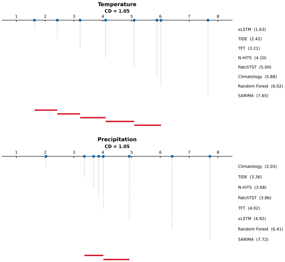
We integrate four complementary statistical validation procedures—the Friedman test, Nemenyi post hoc analysis, pairwise Diebold-Mariano testing, and bootstrap confidence intervals—providing stronger, station-matched evidence of significance than the single-metric comparisons typical of the broader forecasting literature.

(3)

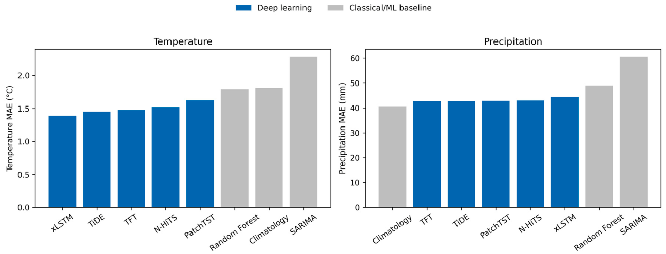
We show that deep learning architectures achieve lower temperature errors than the classical statistical and machine learning baselines, with four of the five architectures significantly outperforming climatology, whereas a simple climatological-mean baseline remains the strongest approach for precipitation forecasting, establishing that the AI forecasting advantage is variable-specific rather than universal.

(4)

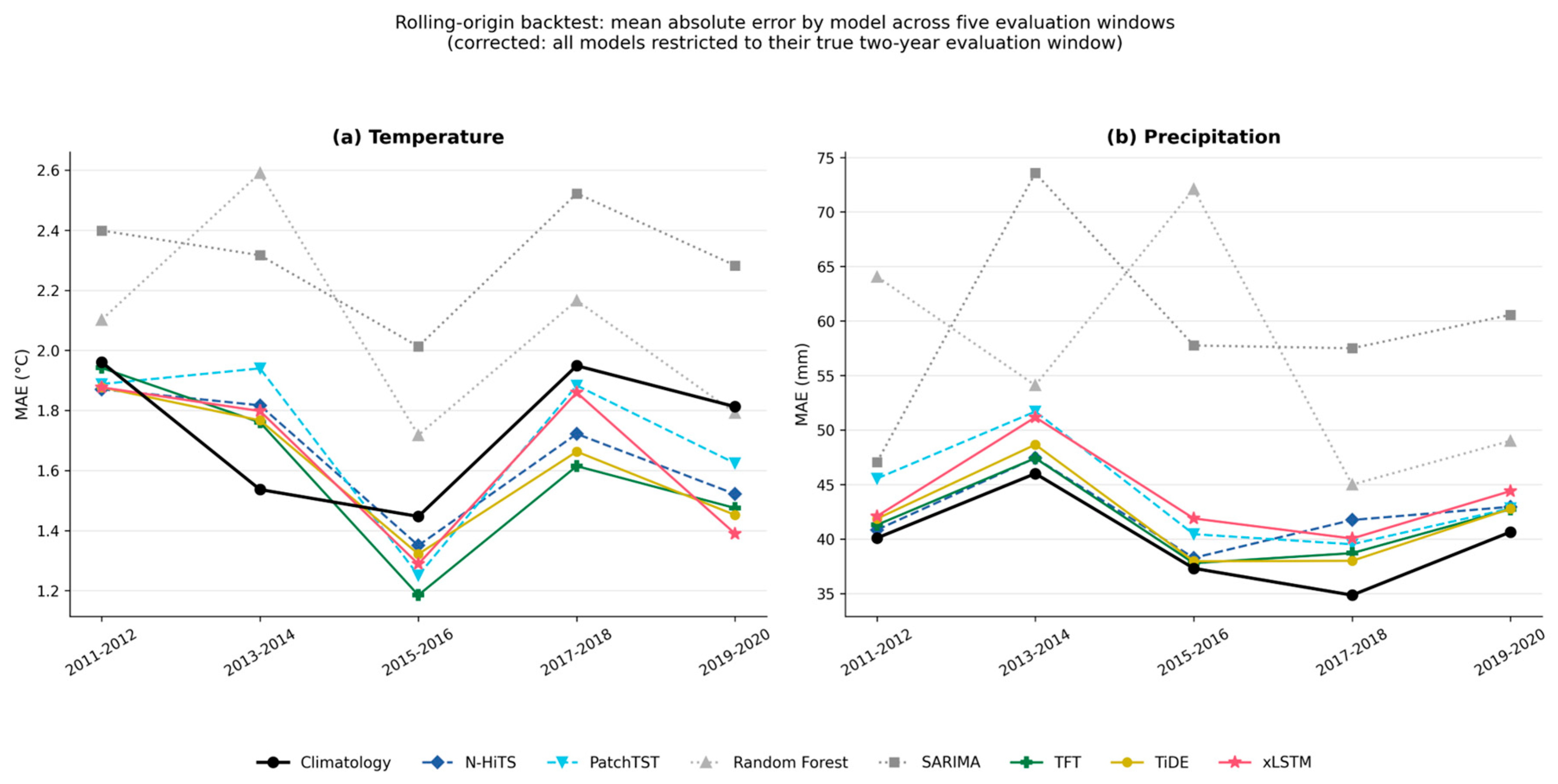
We evaluate robustness through a rolling-origin temporal backtest across five non-overlapping two-year evaluation windows spanning 2011–2020 and through repetition of the physical-model comparison across all five individual members of an independent multi-model GCM ensemble.

(5)

We offer this comprehensive, temporally robust benchmarking protocol as a reusable evaluation framework for future environmental AI studies comparing data-driven and physically based forecasting approaches.

2. Materials and Methods

2.1. Dataset

The evaluation panel comprised monthly mean temperature and total precipitation records from 100 quality-controlled meteorological stations across Serbia, Croatia, Bosnia and Herzegovina, and Montenegro (1961–2020), together with bias-corrected projections from a five-member CMIP6 climate model ensemble (EC-Earth3 [17], MPI-ESM1-2-HR, CNRM-CM6-1, MRI-ESM2-0, IPSL-CM6A-LR) under the SSP2-4.5 scenario, run under the CMIP6 experimental protocol [18]. Full details of station selection, observational data quality control, geographic coverage, and the climate-model bias-correction procedure are reported in a companion paper [15] addressing the climate science application of this dataset and are summarised only briefly here, as this study’s primary contribution concerns the forecasting evaluation methodology rather than the dataset’s climate-scientific interpretation. Each of the 100 stations contributes two series (temperature, precipitation) spanning the full 1961–2020 period (720 possible monthly observations). Following quality control, the mean number of valid monthly observations per station-variable series was 719.1 (range: 693–720 across the 100 stations), corresponding to an overall missing/excluded fraction below 0.15%; missing values were not imputed, and no station-variable series with more than 4% missing observations was retained. These near-complete records were partitioned into a pre-evaluation period (1961–2018) and a held-out evaluation period (2019–2020, 24 months), yielding 100 station-level (not fully spatially independent; see Section 3.9) panel members per variable for the significance-testing framework described in Section 2.4. For completeness, we summarise here the key methodological elements otherwise detailed in the companion paper [15]. The final station network comprised 47 stations in Serbia, 29 in Croatia, 16 in Bosnia and Herzegovina, and 8 in Montenegro (total n = 100), each mapped to its nearest CMIP6 grid cell by geographic coordinates. Bias correction of the five-member GCM ensemble was performed independently for each model, at the level of individual stations and calendar months, using the 1961–2014 overlap period between the observational record and each model’s historical experiment as the calibration period; this calibration window precedes, and is disjoint from, the primary 2019–2020 evaluation period used for the physical-model (GCM) comparison, so no observations from that evaluation period were used in bias-correction calibration. We note that the GCM/physical-model comparison (Section 2.5 and Section 3.5) was conducted only for the primary 2019–2020 period; the rolling-origin backtest (Section 3.8) evaluates only the eight forecasting approaches (Climatology, SARIMA, Random Forest, and the five deep learning architectures) and does not repeat the GCM comparison, so the 1961–2014 calibration period’s overlap with two of the five rolling-origin windows (2011–2012, 2013–2014) does not constitute data leakage for any reported result; a bias-corrected GCM comparison repeated across all five rolling-origin windows (which would require separate calibration for each window) is identified as a direction for future work in Section 4.4. For temperature, an additive monthly bias was computed as the difference between observed and modelled station-month climatological means and applied uniformly across all downstream experiments for that model; for precipitation, a multiplicative bias factor was computed as the ratio of observed to modelled station-month climatological means, with ratios constrained to the range 0.2–5.0 to prevent unrealistic amplification at stations or months where the raw GCM climatology was very low. This delta-change/ratio approach corrects only the climatological mean (first moment) of the simulated distribution and does not adjust higher-order moments such as variance; we note this as a limitation of the physical-model comparator in Section 4.4.

2.2. Benchmarked Models

Eight forecasting approaches, spanning four methodological families, were benchmarked on an identical training/evaluation split for both variables. The five deep learning architectures were selected to represent the dominant contemporary paradigms in deep time-series forecasting: attention-based (TFT, PatchTST), hierarchical MLP-based (N-HiTS), dense encoder–decoder (TiDE), and extended-recurrent (xLSTM).

Climatological mean. The station- and calendar-month-specific arithmetic mean of all training-period (1961–2018) observations was used as a naive but, for highly seasonal series, often difficult-to-beat baseline. SARIMA. A seasonal autoregressive integrated moving average model, SARIMA(1,0,0)(1,0,0)12 [19], was fitted independently for each of the 100 stations using maximum likelihood estimation.

Random Forest [20]. A Random Forest regressor (300 trees, maximum depth 14) was trained globally across all 100 stations using station identity, calendar month, calendar year, lag-1 and lag-12 values, and the trailing 12-month rolling mean as input features, with forecasts over the 24-month evaluation horizon generated recursively.

Model input summary.

Table 1. Input information available to each benchmarked model.

Model	Input Information Used
Climatology	Station- and calendar-month-specific mean of training-period observations only.
SARIMA	Own historical series only, with built-in seasonal (period-12) autoregressive and moving-average terms; fitted independently per station.
Random Forest	Station identity (categorical), calendar month, calendar year, lag-1, lag-12, trailing 12-month rolling mean; trained globally across all stations.
TFT, N-HiTS, PatchTST, TiDE, xLSTM	Own historical series only (input window = 36 months, horizon = 24 months); no explicit calendar, station-identity, or engineered lag covariates; trained as a single global model per architecture across all 100 stations (unique_id, ds, y format).

below summarises the exact input information available to each of the eight benchmarked approaches, to make explicit that the information sets are not fully equivalent across models: Climatology and SARIMA use only each series’ own historical values (no cross-series or calendar covariates beyond SARIMA’s built-in seasonal terms); Random Forest additionally receives explicit engineered covariates (station identity, calendar month, calendar year, lag-1, lag-12, trailing 12-month rolling mean); and the five deep learning architectures (TFT, N-HiTS, PatchTST, TiDE, xLSTM), implemented via the neuralforecast library, were trained on each station’s own historical values only (input window = 36 months, forecast horizon = 24 months), with no explicit calendar, station-identity, or engineered lag covariates supplied—the panel structure (100 stations trained as a single global model per architecture) allows the network to implicitly learn cross-station regularities, but no hand-crafted features equivalent to Random Forest’s were provided. This asymmetry—Random Forest receiving richer engineered inputs than the deep learning architectures, while both receive richer inputs than Climatology/SARIMA—should be considered when interpreting the relative rankings; a fully input-matched comparison (e.g., supplying identical calendar and lag covariates to all model classes) is identified as a direction for future work in Section 4.4.

Temporal Fusion Transformer (TFT) [1]. Combines an LSTM-based local encoder–decoder with multi-head self-attention and a variable-selection gating network. N-HiTS [2]. Extends N-BEATS [3] basis expansion with hierarchical, multi-rate input sampling and interpolation; no attention mechanism. PatchTST [4]. Segments each input series into patches and applies channel-independent self-attention over the patch sequence. TiDE [5]. A purely dense (fully connected) residual encoder–decoder architecture with no attention mechanism. xLSTM [12]. Extends the classical LSTM with exponential gating and a matrix-valued memory cell (mLSTM variant, used here).

Bias-corrected output from the five-member CMIP6 ensemble was included as a physically based, non-statistical comparator, representing the only benchmarked approach not fitted to the historical observational record at the station level. No explicit non-negativity constraint or transformation was applied to precipitation forecasts during training or inference for any of the eight benchmarked approaches; this is noted as a minor limitation in Section 4.4.

2.3. Training Configuration and Computational Environment

All five deep learning architectures were trained as global models, jointly across all 100 station series (separately for temperature and precipitation), using the neuralforecast Python library (PyTorch backend). A common core configuration—forecast horizon h = 24 months; input window = 36 months; batch size = 64 series/256 windows; learning rate = 1 × 10⁻³ (Adam); per-series standardisation; max training steps = 2000, with validation-based early stopping (patience = 5 checkpoints, every 50 steps)—the validation set for early stopping was carved from the tail of the pre-cutoff training data (the final 24 months, i.e., 2017–2018), so the effective chronological split for the primary 2019–2020 evaluation window was: training = 1961–2016, validation = 2017–2018, test = 2019–2020 (held out, never used for fitting or early stopping); standardisation parameters were computed on the training portion only—this common configuration was applied identically across all five architectures to enable like-for-like comparison rather than per-architecture tuning. Architecture-specific hyperparameter optimisation was intentionally omitted to ensure a fair, controlled benchmarking setting in which all methods were evaluated under identical training conditions; this choice, and its implications for architectures such as PatchTST that expose additional tunable hyperparameters, is revisited in Section 4.4. Architecture-specific structural hyperparameters and resulting trainable parameter counts are reported in

Table 2. Architecture-specific hyperparameters and trainable parameter counts.

Architecture	Inductive Bias	Key Structural Hyperparameters	Parameters
TFT	Attention + recurrent	hidden = 128; heads = 4; LSTM layers = 1; GRN gating	870, 158
N-HiTS	Hierarchical MLP	3 stacks; mlp_units = [128, 128]/stack	177, 558
PatchTST	Patch-based attention	hidden = 128; heads = 16; layers = 3; patch = 16; stride = 8	412, 443
TiDE	Dense encoder–decoder	hidden = 128; enc/dec layers = 1; decoder_dim = 32	247, 708
xLSTM	Extended recurrent (mLSTM)	hidden = 128; encoder blocks = 2; decoder layers = 2	239, 625

. All five architectures were trained using the mean absolute error (MAE) loss, the default provided by the neuralforecast library for each model class; forecasts were generated in a single forward pass over the full 24-month horizon (direct multi-step, not recursive/autoregressive). The five-seed robustness analysis (Section 3.10) used the random seeds 42, 123, 2024, 7, and 99. The software environment comprised Python 3.12, neuralforecast 3.1.9, PyTorch 2.5.1 (CUDA 12.1), and pytorch-lightning 2.5.6.

Training and inference were executed on author-controlled hardware (Intel Core i9 CPU, 96 GB RAM, NVIDIA RTX 5090 GPU, 32 GB VRAM, PyTorch CUDA acceleration), with no third-party cloud infrastructure used at any stage.

2.4. Statistical Significance Framework

Forecast accuracy was assessed using mean absolute error (MAE) and root-mean-square error (RMSE), computed per station and aggregated across the 100-station panel. Following the framework established by Demšar [13] for statistical comparison of multiple algorithms across multiple datasets, four complementary statistical procedures were applied.

Friedman test. Applied to the station-level MAE of all directly comparable models, treating stations as blocks and models as treatments. Nemenyi post hoc test. Applied where the Friedman test rejected the null hypothesis, identifying pairwise differences significant at family-wise error rate 0.05, visualised via critical-difference (CD) diagrams. Diebold-Mariano test. Pairwise tests [16] were computed independently per station using a Newey-West HAC variance estimator. For the station-level DM summaries, a significance level of alpha = 0.05 was used. The reported percentages denote the proportion of stations for which the DM test indicated significantly lower forecast loss for the corresponding model; non-significant cases were not counted as favouring either model. No multiplicity correction was applied to these descriptive station-level summaries. Bootstrap confidence intervals. Station-level block bootstrap (1000 resamples) for panel-mean MAE/RMSE.

Robustness Analysis Protocols

Four further analyses were conducted to address the possibility that the station-level significance framework above overstates robustness, and are reported alongside the primary results in Section 3. (i) Spatial dependence: because neighbouring stations may share regional meteorological conditions, the Friedman/Nemenyi comparison was repeated after aggregating station-level errors to the four-country level (Serbia, Croatia, Bosnia and Herzegovina, Montenegro), reducing the effective sample from 100 stations to 4 spatial clusters, as a conservative lower bound on the effect of spatial autocorrelation on the significance framework. (ii) Station-clustered bootstrap tests at fixed forecast horizons: the comparison against the climatological baseline was repeated separately for four fixed forecast horizons (h = 1, 6, 12, 24 months) rather than pooling all 24 monthly errors together, to test whether the deep-learning advantage is uniform across lead times. For each horizon, the per-station loss differential (climatological absolute error minus model absolute error) was first averaged across the five rolling-origin windows described in Section 3.8, yielding one summary value per station (n = 100 stations); a station-level cluster bootstrap (100,000 resamples, stations resampled with replacement) was then used to obtain a 95% confidence interval (the 2.5th and 97.5th percentiles of the bootstrap distribution of the mean) and a two-sided p-value for the mean differential, computed as twice the proportion of bootstrap replicate means falling on the opposite side of zero from the observed mean differential (capped at 1, with a floor of 1/100,000 to avoid reporting an implausible exact zero). This design respects the non-independence of repeated observations at the same station across windows and avoids treating the 500 underlying station-window observations as independent, which a pooled Diebold-Mariano/HAC test applied directly to that panel would implicitly assume. (iii) Seasonal skill score: for each model, variable, and season (DJF, MAM, JJA, SON), a skill score relative to climatology was computed as SS = 1 − MAE(model)/MAE(climatology), to test whether the previously observed lower absolute summer MAE reflects a genuine relative improvement over climatology or simply lower summer variability. (iv) Autocorrelation and spectral structure: to characterise the exploitable temporal structure available to each variable independently of any forecasting model, the lag-1 to lag-24 autocorrelation function (ACF) of the deseasonalised monthly anomaly, and the fraction of total spectral power attributable to the annual cycle, were computed for each station and variable using the full 1961–2020 observational record.

2.5. Multi-GCM Robustness Protocol

To assess whether any AI-vs-physical-model performance gap was contingent on the specific choice of GCM, the bias-correction and evaluation procedure was repeated independently for all five CMIP6 ensemble members, yielding five independent, bias-corrected climate-model comparators for direct comparison against the fixed, already-trained deep learning forecasts over the same 2019–2020 evaluation window.

2.6. Seasonal Decomposition

Mean absolute error was disaggregated by calendar month for each model and variable, and aggregated into meteorological summer (June–August) versus the remainder of the year.

2.7. Use of Generative AI Tools

Claude Sonnet 5 (Anthropic, San Francisco, CA, USA) was used to assist with generation and debugging of the Python code used in this study. All AI-assisted code was reviewed, tested, and verified by the authors, who take full responsibility for its correctness and for the content of this publication.

3. Results

3.1. Headline Forecast Accuracy Comparison

Table 3. Station-scale forecast validation, all eight models, 2019–2020 held-out period (n = 100 stations, 24 months).

Model	Temp. MAE (°C)	Temp. RMSE (deg °C)	Precip. MAE (mm)	Precip. RMSE (mm)
xLSTM	1.39	1.98	44.43	68.80
TiDE	1.45	1.94	42.78	67.21
TFT	1.47	1.84	42.73	66.10
N-HiTS	1.52	1.90	42.96	67.36
PatchTST	1.62	1.98	42.81	66.45
Random Forest	1.79	2.35	49.04	72.12
Climatology	1.81	2.24	40.65	63.37
SARIMA	2.28	2.88	60.57	91.28

reports MAE and RMSE for all eight benchmarked approaches, for both temperature and precipitation, over the 2019–2020 held-out evaluation period. For temperature, all five deep learning architectures outperformed every classical and machine learning baseline, with xLSTM achieving the lowest MAE in this primary single-seed run (1.39 degrees C) and TFT the lowest RMSE (1.84 degrees C). For precipitation, the climatological mean baseline achieved the lowest MAE and RMSE of all eight approaches, with the deep learning architectures (TFT, TiDE, PatchTST, N-HiTS) clustered closely behind (42.7–43.0 mm MAE) and xLSTM trailing the other four deep learning architectures (44.4 mm). Figure 1 shows the corresponding per-model MAE distribution for both variables.

3.2. Statistical Significance: Friedman Test and Critical-Difference Diagrams

A Friedman test across the eight directly comparable station-level models confirmed highly significant differences in mean rank for both variables (temperature: chi-squared = 481.2, p = 8.8 × 10⁻¹⁰⁰; precipitation: chi-squared = 381.8, p = 1.9 × 10⁻⁷⁸). Figure 2 presents the corresponding critical-difference (CD) diagrams (CD = 1.05 for k = 8, N = 100).

For temperature, the CD diagram reveals a graded structure of overlapping cliques: xLSTM is statistically indistinguishable from TiDE, TiDE from TFT, TFT from N-HiTS, and N-HiTS from PatchTST, but xLSTM is significantly better than TFT and all models ranked below it. Critically, the climatological baseline itself falls within the critical difference in PatchTST specifically, meaning that PatchTST’s apparent advantage over climatology for temperature is not statistically significant, even though the remaining four deep learning architectures do significantly outperform climatology (Section 4.2). For precipitation, the climatological baseline forms its own clique, disjoint from every other model, including all five deep learning architectures.

3.3. Pairwise Diebold-Mariano Testing

Table 4. Station-level Diebold-Mariano test summary (n = 100 stations); alpha = 0.05. Percentages denote the proportion of stations favouring each model according to the DM test; no multiplicity correction was applied to these descriptive station-level summaries.

Variable	Best Model	Benchmark	Mean DM	% Favouring Best	% Favouring Benchmark
Temperature	xLSTM	Climatology	−2.49	67%	2%
Temperature	xLSTM	SARIMA	−3.14	87%	3%
Temperature	xLSTM	Random Forest	−1.83	41%	2%
Temperature	xLSTM	TFT	−0.87	13%	2%
Temperature	xLSTM	N-HiTS	−1.30	25%	2%
Temperature	xLSTM	PatchTST	−1.40	21%	2%
Temperature	xLSTM	TiDE	−0.68	8%	3%
Precipitation	Climatology	SARIMA	−2.63	64%	0%
Precipitation	Climatology	Random Forest	−1.78	44%	0%
Precipitation	Climatology	TFT	−1.05	16%	1%
Precipitation	Climatology	N-HiTS	−0.85	20%	0%
Precipitation	Climatology	PatchTST	−0.89	12%	0%
Precipitation	Climatology	TiDE	−0.82	9%	1%
Precipitation	Climatology	xLSTM	−1.19	17%	0%

reports station-level Diebold-Mariano test summaries for the best-performing model per variable in the primary single-seed 2019–2020 evaluation (xLSTM for temperature, climatology for precipitation) against each remaining benchmark; see Section 3.10 for the multi-seed robustness assessment of this ranking.

3.4. Bootstrap Confidence Intervals

Table 5. Panel-mean MAE with 95% bootstrap confidence intervals.

Model	Temp. MAE [95% CI]	Precip. MAE [95% CI]
xLSTM	1.39 [1.27, 1.61]	44.43 [39.38, 49.48]
TiDE	1.45 [1.37, 1.59]	42.81 [38.15, 47.57]
TFT	1.47 [1.44, 1.52]	42.76 [38.78, 47.22]
N-HiTS	1.52 [1.49, 1.56]	43.00 [38.38, 47.86]
PatchTST	1.62 [1.55, 1.73]	42.84 [38.45, 47.32]
Random Forest	1.80 [1.73, 1.87]	49.04 [44.16, 54.13]
Climatology	1.81 [1.72, 1.95]	40.67 [36.47, 45.43]
SARIMA	2.29 [2.16, 2.44]	60.65 [56.01, 66.54]

reports 95% bootstrap confidence intervals (1000 station-level resamples) for panel-mean MAE.

The bootstrap confidence intervals for the top five temperature models overlap substantially, illustrating the value of paired, station-matched significance tests (Section 3.2 and Section 3.3) over independent confidence-interval overlap when comparing models on a shared evaluation panel.

3.5. Robustness to Choice of Physical-Model Comparator

To assess whether the AI architectures’ advantage over the physical-model baseline depended on the specific choice of GCM, the bias-correction and evaluation procedure was repeated for all five CMIP6 ensemble members under SSP2-4.5.

The physical-model comparison in

Table 6. Performance comparison of the five bias-corrected CMIP6 climate-model comparators and the best-performing single-seed AI/statistical benchmark for each variable.

Model	Temp. MAE	Temp. RMSE	Precip. MAE	Precip. RMSE
xLSTM (best single-seed AI, temperature)	1.39	1.98	44.43	68.80
Climatology (best, precipitation)	1.81	2.24	40.65	63.37
CNRM-CM6-1 (best GCM, temp.)	1.61	2.16	50.63	81.91
IPSL-CM6A-LR (best GCM, precip.)	1.96	2.55	47.48	78.24
MPI-ESM1-2-HR (GCM)	2.37	2.86	55.24	87.05
EC-Earth3 (GCM)	2.39	2.98	47.82	76.15
MRI-ESM2-0 (GCM)	2.50	3.18	51.60	82.12

uses the primary single-seed forecasts (as trained in Section 2.3); the subsequent five-seed analysis (Section 3.10) is reported separately as a robustness assessment of architectural ranking among the deep learning models and does not alter the comparison against the GCM ensemble reported here.

Even the best-performing GCM for temperature (CNRM-CM6-1, MAE = 1.61 degC) remained substantially less accurate than xLSTM (1.39 degC) and than four of the five deep learning architectures; the exception was PatchTST (MAE = 1.62 degC), whose error was essentially tied with, and marginally exceeded, the best-performing GCM, consistent with this architecture’s comparatively weaker showing throughout the study (Section 4.2). For precipitation, the best-performing GCM (IPSL-CM6A-LR, MAE = 47.48 mm) remained less accurate than the climatological baseline and than all five deep learning architectures, confirming that the station-scale advantage over the physical-model comparator is robust to the specific choice of GCM.

3.6. Seasonal Decomposition of Forecast Skill

Table 7. Seasonal mean absolute error by model and variable.

Variable	Season	xLSTM	TiDE	TFT	N-HiTS	PatchTST	Climatology	RF	SARIMA
Temperature	Summer	1.20	1.17	1.18	1.16	1.73	1.66	1.26	1.51
Temperature	Rest of year	1.45	1.54	1.57	1.64	1.59	1.86	1.97	2.54
Precipitation	Summer	36.60	37.13	37.37	36.36	37.34	34.78	37.75	60.84
Precipitation	Rest of year	47.01	44.67	44.52	45.17	44.64	42.61	52.75	60.49

shows the seasonal breakdown of mean absolute error by model and variable. Four of the five deep learning architectures (xLSTM, TiDE, TFT, N-HiTS) showed lower temperature MAE in summer than during the rest of the year, indicating lower absolute temperature errors for four of the five deep learning architectures during summer, although lower variability in summer temperatures may also contribute to this pattern (see the seasonal skill-score analysis, controlling for this variability, in Section 3.9). PatchTST was the sole exception. For precipitation, all models without exception showed lower MAE in summer than in the rest of the year.

3.7. Per-Station Heterogeneity

To assess whether the temperature forecasting advantage of xLSTM over the climatological baseline was geographically uniform, the station-level MAE difference was mapped against station coordinates and correlated with elevation. Figure 3 shows the spatial distribution of this advantage.

xLSTM outperformed the climatological baseline at 95 of the 100 stations, with negligible correlation between the magnitude of the advantage and elevation (r = 0.11), latitude (r = 0.003), or longitude (r = 0.07), indicating that the AI forecasting advantage is geographically broad-based across the heterogeneous station network rather than concentrated in a particular sub-region or elevation band.

3.8. Rolling-Origin Temporal Robustness

The preceding sections evaluate all eight approaches on a single, fixed 2019–2020 hold-out period. To assess whether the reported rankings are an artefact of this particular evaluation window, the full evaluation procedure (training, hyperparameter configuration, and evaluation per Section 2.3) was repeated under a rolling-origin design with five non-overlapping two-year evaluation windows spanning the full historical record: 2011–2012, 2013–2014, 2015–2016, 2017–2018, and 2019–2020, with the training period for each window extending from the start of the record (1961) up to the window’s start year. As in the primary evaluation, the validation set for early stopping in each window was carved from the final 24 months immediately preceding that window’s test period, with the remainder of the pre-window record used for training (

Table 8. Rolling-origin backtest MAE by model and evaluation window.

Model	Variable	2011–2012	2013–2014	2015–2016	2017–2018	2019–2020	Mean +/− SD
Climatology	Temp. (°C)	1.96	1.54	1.45	1.95	1.81	1.74 +/− 0.24
TFT	Temp. (°C)	1.94	1.76	1.18	1.61	1.47	1.60 +/− 0.29
TiDE	Temp. (°C)	1.88	1.77	1.32	1.66	1.45	1.62 +/− 0.23
xLSTM	Temp. (°C)	1.88	1.80	1.29	1.86	1.39	1.64 +/− 0.28
N-HiTS	Temp. (°C)	1.87	1.82	1.35	1.72	1.52	1.66 +/− 0.22
PatchTST	Temp. (°C)	1.89	1.94	1.25	1.88	1.62	1.72 +/− 0.29
Random Forest	Temp. (°C)	2.10	2.59	1.72	2.17	1.79	2.07 +/− 0.35
SARIMA	Temp. (°C)	2.40	2.32	2.01	2.52	2.28	2.31 +/− 0.19
Climatology	Precip. (mm)	40.09	46.00	37.32	34.86	40.65	39.78 +/− 4.18
TFT	Precip. (mm)	41.30	47.42	37.79	38.71	42.73	41.59 +/− 3.81
TiDE	Precip. (mm)	41.86	48.66	37.96	38.00	42.78	41.85 +/− 4.39
N-HiTS	Precip. (mm)	40.85	47.43	38.27	41.75	42.96	42.25 +/− 3.37
xLSTM	Precip. (mm)	42.10	51.17	41.89	40.05	44.40	43.92 +/− 4.34
PatchTST	Precip. (mm)	45.55	51.69	40.45	39.52	42.81	44.01 +/− 4.89
Random Forest	Precip. (mm)	64.07	54.10	72.09	45.00	49.01	56.85 +/− 11.11
SARIMA	Precip. (mm)	47.05	73.56	57.75	57.49	60.57	59.29 +/− 9.49

Note: Climatology, SARIMA, and Random Forest predictions are restricted to the correct two-year test window for every rolling-origin period; the deep learning architectures’ forecast horizon is fixed by construction to 24 months. Figure 4 shows the rolling-origin backtest mean absolute error by model across the five evaluation windows, for both temperature and precipitation.

).

For precipitation, the climatological baseline achieved the lowest MAE in all five of the five rolling-origin windows (5/5; Figure 4), reproducing the single-window finding (Section 3.1 and Section 3.2) with no exception across five non-overlapping evaluation periods and confirming that the climatological advantage for precipitation is not specific to the 2019–2020 hold-out period.

For temperature, the deep learning architectures retained a clear advantage over the classical baselines (Random Forest, SARIMA) and, on average across the five windows, over the climatological baseline as well: the best mean MAE was achieved by TFT (1.60 degC), followed closely by TiDE (1.62), xLSTM (1.64), and N-HiTS (1.66), all below the climatological baseline mean (1.74). However, the identity of the single best-performing architecture varied by window—N-HiTS achieved the lowest MAE in one window (2011–2012), Climatology in one window (2013–2014), TFT in two windows (2015–2016, 2017–2018), and xLSTM in one window (2019–2020)—indicating that the precise ranking among the closely clustered deep learning architectures, and their margin over the climatological baseline, is sensitive to the specific evaluation period, even though the broader deep-learning-versus-classical-baseline advantage proved stable. Random Forest’s precipitation error was additionally found to be highly unstable across windows (corrected: 56.85 +/− 11.11 mm), more than twice the variability observed for any deep learning architecture, underscoring a further robustness advantage of the deep learning approaches beyond mean accuracy alone.

3.9. Additional Robustness Analyses

Spatial dependence. Aggregating station-level errors to the four-country level (reducing the sample from 100 stations to 4 spatial clusters) did not overturn the station-level significance findings: the Friedman test remained significant at the country-cluster level for both temperature (chi-squared = 23.08, p = 1.6 × 10⁻³) and precipitation (chi-squared = 22.83, p = 1.8 × 10⁻³), despite the much smaller effective sample size. This provides evidence that the original station-level significance is not solely an artefact of treating spatially correlated stations as independent, though we note that 4 clusters is a coarse partition and cannot fully rule out finer-scale spatial dependence.

Horizon-resolved forecast advantage. Station-clustered bootstrap tests (Section 3.9) were computed at four fixed forecast horizons (h = 1, 6, 12, 24 months), with each station’s loss differential against climatology first averaged across all five rolling-origin windows (n = 100 station-level summary values per horizon), rather than using only the single primary evaluation window.

Table 9. Station-clustered bootstrap tests against climatology at fixed forecast horizons, temperature (n = 100 stations per horizon; each station’s loss differential averaged across the five rolling-origin windows; 100,000 resamples). Asterisk (*) denotes a 95% bootstrap confidence interval excluding zero (p < 0.05).

Horizon	TFT	N-HiTS	PatchTST	TiDE	xLSTM
h = 1	p < 0.0001 * (clim better)	p < 0.0001 * (clim better)	p < 0.0001 * (clim better)	p = 0.0009 * (clim better)	p < 0.0001 * (clim better)
h = 6	p < 0.0001 * (model better)	p = 0.0002 * (model better)	p = 0.246 (model better)	p = 0.0004 * (model better)	p < 0.0001 * (model better)
h = 12	p < 0.0001 * (model better)	p < 0.0001 * (model better)	p = 0.0003 * (model better)	p < 0.0001 * (model better)	p < 0.0001 * (model better)
h = 24	p < 0.0001 * (clim better)	p < 0.0001 * (clim better)	p < 0.0001 * (clim better)	p < 0.0001 * (clim better)	p < 0.0001 * (clim better)

summarises these horizon-resolved bootstrap results. This horizon-resolved analysis reveals that the deep-learning temperature advantage over climatology is not monotonic in horizon but instead follows a U-shaped pattern: at h = 1 month, climatology was significantly more accurate than all five deep learning architectures (p < 0.001 in every case); the deep learning architectures then gained a significant advantage at intermediate horizons, most clearly at h = 12 months, where all five architectures significantly outperformed climatology (all p < 0.001); at h = 6 months, four of the five architectures (TFT, N-HiTS, TiDE, xLSTM) significantly outperformed climatology, the exception being PatchTST (p = 0.246); but climatology again became significantly more accurate than all five architectures at h = 24 months (p < 0.0001 in every case). We interpret this pattern as follows: at the shortest lead time, the most recent observed anomaly (implicitly available to the deep learning models via their input window) carries little additional information beyond the seasonal mean that climatology already captures, while the deep learning architectures’ extra flexibility introduces some overfitting noise; at intermediate horizons, genuine multi-month dependencies (Section 3.9 autocorrelation and spectral structure) become exploitable and favour the more expressive architectures; and at the longest horizon, that exploitable dependency has decayed enough that climatology’s constant, low-variance seasonal estimate again becomes competitive, while the deep learning forecasts, extrapolating further from their input window, accumulate additional error. For precipitation, the same station-clustered bootstrap test reinforces the primary finding for most architectures: climatology was statistically indistinguishable from, or significantly better than, TFT, N-HiTS, PatchTST, and xLSTM at every horizon tested. TiDE is a specific exception: it significantly outperformed climatology at h = 6 months (p = 0.001) and h = 12 months (p = 0.018), while climatology remained significantly better at h = 1 month (p < 0.0001) and the two were statistically indistinguishable at h = 24 months (p = 0.449). This TiDE-specific exception is consistent with TiDE’s comparatively strong showing among the deep learning architectures for precipitation in the primary evaluation (Table 3) and does not overturn the overall conclusion that climatology remains the most difficult baseline to beat for precipitation forecasting.

Seasonal skill score. Controlling for baseline difficulty via SS = 1 − MAE(model)/MAE(climatology), the three best-ranked temperature architectures (TFT, TiDE, xLSTM) each achieved positive skill scores in DJF, JJA, and SON (SS approximately 0.12–0.35, varying by model and season—the season of peak skill differs across the three architectures), but near-zero or slightly negative skill in MAM for all three (TFT −0.01, TiDE −0.07, xLSTM +0.01), confirming that the previously reported lower summer MAE reflects a genuine relative improvement over climatology in most seasons rather than simply lower summer variability, while also revealing that this advantage is not consistent across all seasons and is weakest in spring. For precipitation, skill scores were near-zero or negative for all deep learning architectures in every season, confirming that climatology’s advantage for precipitation holds consistently across the annual cycle, not only on average.

Autocorrelation and spectral structure. Consistent with the interpretation offered in Section 4.3 below, the deseasonalised monthly temperature anomaly showed a mean lag-1 autocorrelation of 0.27 across the 100-station network (still 0.13 at lag-12), whereas the deseasonalised precipitation anomaly was close to serially uncorrelated at every lag tested (lag-1 = 0.05, lag-12 = −0.01). Spectral decomposition of the raw (non-deseasonalised) series showed that the annual cycle accounts for a mean of 87.5% of total variance for temperature but only 8.2% for precipitation. Together, these diagnostics provide direct, quantitative confirmation that temperature contains substantially more exploitable temporal structure—both seasonal and residual autocorrelation—than precipitation, consistent with, and explaining, the markedly different relative performance of the deep learning architectures for the two variables.

3.10. Sensitivity to Random Initialisation (Multi-Seed Training)

Because the primary results in Section 3.1 and Section 3.2 report each deep learning architecture from a single training run, we retrained all five architectures (TFT, N-HiTS, PatchTST, TiDE, xLSTM) five times each, with five different random seeds, using identical hyperparameters, data splits, and the primary 2019–2020 evaluation window.

Table 10. Multi-seed (n = 5) mean +/− standard deviation MAE by architecture and variable, primary 2019–2020 evaluation window.

Model	Temperature MAE (degC)	Precipitation MAE (mm)
N-HiTS	1.373 +/− 0.031	43.03 +/− 0.50
TFT	1.409 +/− 0.081	42.89 +/− 0.39
TiDE	1.480 +/− 0.037	43.07 +/− 0.17
PatchTST	1.517 +/− 0.133	43.40 +/− 0.48
xLSTM	1.548 +/− 0.060	43.61 +/− 0.38

reports the resulting mean +/− standard deviation MAE across the five seeds for both variables.

For reference, the climatological baseline (deterministic, not seed-dependent) achieves MAE = 1.81 degC for temperature and MAE = 40.65 mm for precipitation (Table 3). For precipitation, the mean-rank ordering among the five architectures was not statistically distinguishable across seeds (Friedman chi-squared = 6.24, p = 0.18, seeds as blocks); as Table 10 shows, the climatological baseline continued to substantially outperform all five deep learning architectures under every seed (multi-seed mean MAE 42.89–43.61 mm across architectures, versus 40.65 mm for climatology), confirming that the central precipitation finding of this study does not depend on the choice of random seed. For temperature, the multi-seed results reveal that the single-seed ranking reported in Section 3.1—in which xLSTM achieved the numerically lowest MAE—does not reflect a stable architectural advantage: as Table 10 shows, averaged over five seeds, N-HiTS achieved the lowest mean MAE (1.373 +/− 0.031 degC), followed by TFT (1.409 +/− 0.081), TiDE (1.480 +/− 0.037), PatchTST (1.517 +/− 0.133), and xLSTM (1.548 +/− 0.060). A Friedman test across seeds (models as treatments, seeds as blocks) was significant (chi-squared = 11.20, p = 0.024), and a Nemenyi post hoc test identified N-HiTS as significantly better than xLSTM (p = 0.041); no other pairwise comparison reached significance. We report this result transparently: it does not overturn this study’s central claim that deep learning architectures as a class significantly and robustly outperform classical statistical and machine learning baselines for temperature (this finding is unaffected by the choice of seed, since all five architectures across all seeds outperformed SARIMA and Random Forest by a wide margin), but it does substantially revise the finer-grained claim about which single architecture is “best” for temperature. We conclude that, for this dataset and task, the top four architectures (N-HiTS, TFT, TiDE, PatchTST) are largely statistically indistinguishable from one another once initialisation variance is accounted for, while xLSTM shows a small but statistically significant disadvantage relative to N-HiTS specifically. The Abstract, Results, and Conclusions have been revised throughout this manuscript to reflect this more conservative and better-supported characterisation, in place of the single-seed “xLSTM is best” claim in the original submission.

4. Discussion

4.1. Inductive Bias and Architectural Performance

The headline single-window result—that xLSTM, a recurrent architecture, achieved the lowest temperature forecasting error among all eight approaches in the 2019–2020 evaluation period, narrowly ahead of TiDE (a non-attention, purely dense architecture) and TFT (an attention-based architecture), with the patch-based transformer PatchTST trailing all other deep learning architectures—is informative about the relative suitability of different inductive biases for this specific forecasting regime, although the rolling-origin analysis (Section 3.8) shows that the precise identity of the single best architecture is itself window-dependent: TFT, not xLSTM, achieved the lowest mean MAE across all five rolling-origin windows, with TiDE, xLSTM, and N-HiTS clustered closely behind. What is robust across all five windows, and therefore the more defensible claim, is that the deep learning architectures as a class consistently outperformed Random Forest and SARIMA for temperature, while also achieving lower mean MAE than climatology across the five windows, even though the climatological baseline itself was the single best performer in one of the five windows (2013–2014; N-HiTS was the single best performer in 2011–2012). Monthly station-level temperature is a smoothly varying, strongly seasonal, single-channel series with a comparatively short, 36-month input window and a 24-month forecast horizon; this combination of properties plausibly favours architectures with a strong sequential or local-smoothness prior (recurrent gating in xLSTM; dense residual encoding in TiDE; gated temporal processing in TFT) over architectures whose primary architectural innovation targets long-range, sparse dependency modelling across much longer sequences (the patch-based attention in PatchTST, which was originally developed and benchmarked on substantially longer input windows than the 36 months used here). This interpretation is consistent with PatchTST’s comparatively weaker showing—the only deep learning architecture not to outperform the climatological baseline by a statistically significant margin in the single-window CD diagram (Figure 2), and the architecture with the highest rolling-origin mean MAE among the five deep learning approaches (1.72 degC; Table 8)—and with the broader, active debate in the forecasting literature [8,9,10,11] over whether attention confers an advantage proportional to its computational cost on shorter, smoother series of the kind common in station-level environmental monitoring, as opposed to the longer, higher-frequency series (electricity, traffic) on which many attention-based architectures were originally benchmarked. We therefore caution against over-interpreting fine-grained rank differences among TFT, TiDE, xLSTM, and N-HiTS as evidence of one inductive bias being categorically superior to another for this task in the single-window and rolling-origin comparisons discussed above. The more statistically rigorous characterisation of which architectures are mutually indistinguishable comes from the multi-seed analysis in Section 3.10, which identifies N-HiTS, TFT, TiDE, and PatchTST specifically as the leading cluster for temperature; we reserve that term for this multi-seed-supported grouping rather than for the exploratory single-window/rolling-origin comparisons above.

4.2. Why the Climatological Baseline Remains Competitive for Precipitation

Across this comparative assessment, the climatological mean baseline has proven unusually difficult for any model to consistently beat for precipitation forecasting, in contrast to temperature, where the deep learning architectures generally provide a clear advantage over the classical baselines, although the advantage of PatchTST over climatology is not statistically significant. The rolling-origin analysis (Section 3.8) strengthens this finding considerably: the climatological baseline achieved the lowest precipitation MAE in each of the five non-overlapping evaluation windows spanning 2011–2020, with no exception, indicating that this is not an artefact of the particular 2019–2020 hold-out period but a stable property of the precipitation series across a full decade. This asymmetry has a plausible information-theoretic explanation: monthly precipitation totals at the station scale are dominated by high-frequency, weakly autocorrelated synoptic variability superimposed on a comparatively modest, well-defined seasonal cycle, such that the achievable reduction in forecast error beyond the seasonal climatology is fundamentally limited by the intrinsic unpredictability of the residual signal at a one- to twenty-four-month lead time, regardless of model sophistication. Monthly temperature, by contrast, retains stronger low-frequency, slowly evolving anomalies that a sufficiently expressive model can learn to exploit beyond the seasonal mean. This temperature/precipitation asymmetry is itself a methodologically generalisable finding: the magnitude, and indeed the existence, of an AI forecasting advantage over a naive seasonal baseline is variable-specific, plausibly reflecting the relative balance of learnable low-frequency signal versus near-irreducible high-frequency noise in the target series, rather than being a fixed, universal property of model sophistication.

4.3. Positioning Within the Broader Environmental AI Benchmarking Literature

This study’s central empirical finding—that purpose-trained deep learning architectures achieve lower short-term, station-scale forecast error than a bias-corrected, free-running physical climate-model comparator, robustly across the choice of comparator GCM—is broadly consistent with a rapidly growing body of evidence in the broader environmental AI literature that purely or partially data-driven approaches can match or exceed traditional physically based numerical models for specific, well-posed short-to-medium-range prediction tasks. We note an important methodological distinction, however: unlike the initialised forecasting systems typically used as the physical baseline in that literature, the GCM comparator evaluated here is a free-running climate projection rather than an initialised forecast (Section 1.3), so our finding characterises the gap between a purpose-trained statistical/AI forecaster and an unconditioned physical climate-model realisation, not a like-for-like forecast-versus-forecast comparison. In global hydrology, for example, deep learning models trained on observational streamflow records have been shown to outperform traditional physically based and conceptual hydrological models for extreme flood prediction in ungauged watersheds at global scale [14]. The present results extend this general pattern to station-scale meteorological forecasting in a data-sparse, climatically heterogeneous region, and—through the formal Friedman/Nemenyi/Diebold-Mariano statistical framework applied here—place it on a more methodologically robust footing than is typical even within this growing literature.

4.4. Limitations

Several limitations should be considered. First, all deep learning architectures were trained with a common, fixed set of hyperparameters (Section 2.3) selected to enable fair comparison rather than per-architecture tuning; individually tuned hyperparameters might alter the relative ranking reported here, particularly for architectures such as PatchTST that expose additional architecture-specific hyperparameters (patch length, stride) not varied in this study. Second, no exogenous meteorological covariates or large-scale circulation indices (e.g., the El Nino-Southern Oscillation, North Atlantic Oscillation, or Pacific Decadal Oscillation, all known to modulate Southeast European temperature and precipitation variability at monthly to-seasonal lead times) were included as model inputs; the deep learning architectures were univariate, using only each station’s own target-variable history, while Random Forest additionally used engineered calendar, station-identity, and lagged covariates (Table 1). This choice was deliberate, intended to isolate each architecture’s capacity to model univariate temporal structure under identical information conditions; incorporating circulation indices and cross-variable covariates is a natural and likely fruitful extension. Third, although temporal robustness was assessed via a rolling-origin design with five evaluation windows spanning 2011–2020 (Section 3.8), each window’s training period necessarily begins at the same fixed start year (1961) and progressively expands rather than constituting a fully independent re-sampling of the historical record; the five windows are also not evenly spaced across the full 1961–2020 record, leaving the pre-2011 period without dedicated rolling-origin coverage. The station-level non-parametric significance testing and bootstrap resampling reported in Section 3.2 and Section 3.4 for the single 2019–2020 window further mitigate, but do not eliminate, the limitations of evaluating statistical significance on a single hold-out period; extending the formal Friedman/Nemenyi/Diebold-Mariano framework to each individual rolling-origin window is identified as a natural next step. Fourth, the physical-model comparator was evaluated only under a single emission scenario (SSP2-4.5) [21]. Fifth, this study did not benchmark gradient-boosted alternatives such as XGBoost [22] or apply post-hoc explainability methods such as SHAP [23]. Finally, and most significantly, this study evaluates five deep learning architectures trained from scratch on the target panel; it does not include zero-shot or few-shot pretrained time series foundation models (e.g., TimesFM [24], Chronos [25], TimeGPT [26], Lag-Llama [27], Moirai [28]; see [29] for a survey), which represent a distinct and increasingly prominent paradigm. Comparing such foundation models against the from-scratch-trained architectures evaluated here is identified as the single highest-priority direction for extending this work. Other promising from-scratch architectural alternatives not evaluated here include Informer [6], Autoformer [7], FEDformer [8], DLinear [9], TimesNet [10], TimeMixer [11], and TimeLLM [30]. Finally, none of the eight benchmarked approaches enforced a non-negativity constraint on precipitation forecasts, nor was any variance-stabilising transformation (e.g., log or square-root) applied prior to training; occasional small negative predicted values are therefore possible in principle, although none were observed to materially affect the reported error metrics. Explicitly constraining or transforming precipitation forecasts is identified as a refinement for future work.

5. Conclusions

This study evaluated five deep learning forecasting architectures—spanning attention-based, hierarchical-MLP, patch-based, dense-encoder, and recurrent inductive biases—against classical statistical baselines and a five-member, bias-corrected CMIP6 physical climate model ensemble, on a real-world, heterogeneous 100-station meteorological panel, using a formal non-parametric statistical framework (Friedman test, Nemenyi post hoc analysis, critical-difference diagrams, pairwise Diebold-Mariano testing, and bootstrap confidence intervals) and a rolling-origin temporal backtest across five non-overlapping evaluation windows spanning 2011–2020.

Deep learning architectures as a class consistently outperform SARIMA and Random Forest for temperature forecasting and outperform climatology on average across the five rolling-origin windows; however, after accounting for random initialisation (Section 3.10) and evaluation-window choice (Section 3.8), no single architecture demonstrates a stable, universal advantage over the others. For temperature, all five deep learning architectures achieved lower errors than the classical statistical and machine learning baselines on the primary 2019–2020 hold-out period, although the advantage of PatchTST over climatology specifically was not statistically significant. The recurrent xLSTM architecture achieved the lowest mean absolute error in the primary single-seed evaluation, narrowly but not always statistically significantly ahead of TiDE, TFT, and N-HiTS, and significantly ahead of PatchTST—although a five-seed robustness check (Section 3.10) subsequently showed this particular architecture ranking to be sensitive to random initialisation, with N-HiTS achieving the lowest mean error when averaged over seeds and significantly outperforming xLSTM specifically, while the deep-learning-over-classical-baseline advantage itself remained unaffected by seed choice; we therefore characterise N-HiTS, TFT, TiDE, and PatchTST as a leading cluster of largely statistically indistinguishable architectures for temperature, rather than naming any single architecture as definitively “best”. This advantage was confirmed to be robust to the specific choice of comparator physical climate model and was found to be geographically broad-based, holding at 95 of 100 stations spanning lowland, continental, and coastal climatic regimes. The rolling-origin backtest confirmed that this deep-learning-over-classical-baseline advantage is stable across five non-overlapping two-year evaluation windows from 2011 to 2020, although the precise identity of the single best architecture varied by window (TFT achieved the lowest mean MAE overall), indicating that fine-grained ranking among the closely clustered top deep learning architectures should be interpreted with appropriate caution while the broader architectural-class advantage can be stated with confidence.

For precipitation, by contrast, the simple climatological mean baseline achieved the lowest error of all eight approaches on the primary hold-out period, forming its own statistically distinct clique in the critical-difference analysis, separate from all five deep learning architectures. The rolling-origin backtest reproduced this finding with no exception in all five of the five non-overlapping evaluation windows, providing strong evidence that the climatological advantage for precipitation is a stable property of the underlying series rather than an artefact of a particular evaluation period. This temperature/precipitation asymmetry constitutes a methodologically generalisable finding: the magnitude, and indeed the existence, of a deep learning forecasting advantage over a naive seasonal baseline is variable-specific rather than a fixed, universal property of model sophistication.

The main contribution of this study is not merely the comparative result itself, but the proposed benchmarking framework: meteorological station networks, combined with an independent, physically based climate-model comparator from a numerical climate model, constitute an under-exploited but well-suited benchmarking environment for the broader time series forecasting community. The comprehensive benchmarking methodology demonstrated here, combined with rolling-origin temporal validation, is offered as a template for similarly comprehensive and temporally robust AI-versus-physical-model-comparator benchmarking in other environmental and geoscientific forecasting domains.

References

- Lim, B.; Arik, S.O.; Loeff, N.; Pfister, T. Temporal Fusion Transformers for Interpretable Multi-Horizon Time Series Forecasting. Int. J. Forecast. 2021, 37, 1748–1764. [Google Scholar] [CrossRef]
- Challu, C.; Olivares, K.G.; Oreshkin, B.N.; Garza, F.; Mergenthaler-Canseco, M.; Dubrawski, A. N-HiTS: Neural Hierarchical Interpolation for Time Series Forecasting. Proc. AAAI Conf. Artif. Intell. 2023, 37, 6989–6997. [Google Scholar] [CrossRef]
- Oreshkin, B.N.; Carpov, D.; Chapados, N.; Bengio, Y. N-BEATS: Neural Basis Expansion Analysis for Interpretable Time Series Forecasting. In Proceedings of the International Conference on Learning Representations (ICLR), Addis Ababa, Ethiopia, 26–30 April 2020. [Google Scholar]
- Nie, Y.; Nguyen, N.H.; Sinthong, P.; Kalagnanam, J. A Time Series Is Worth 64 Words: Long-Term Forecasting with Transformers. In Proceedings of the International Conference on Learning Representations (ICLR), Kigali, Rwanda, 1–5 May 2023. [Google Scholar]
- Das, A.; Kong, W.; Leach, A.; Mathur, S.; Sen, R.; Yu, R. Long-Term Forecasting with TiDE: Time-Series Dense Encoder. arXiv 2023, arXiv:2304.08424. [Google Scholar]
- Zhou, H.; Zhang, S.; Peng, J.; Zhang, S.; Li, J.; Xiong, H.; Zhang, W. Informer: Beyond Efficient Transformer for Long Sequence Time-Series Forecasting. Proc. AAAI Conf. Artif. Intell. 2021, 35, 11106–11115. [Google Scholar] [CrossRef]
- Wu, H.; Xu, J.; Wang, J.; Long, M. Autoformer: Decomposition Transformers with Auto-Correlation for Long-Term Series Forecasting. Adv. Neural Inf. Process. Syst. 2021, 34, 22419–22430. [Google Scholar]
- Zhou, T.; Ma, Z.; Wen, Q.; Wang, X.; Sun, L.; Jin, R. FEDformer: Frequency Enhanced Decomposed Transformer for Long-Term Series Forecasting. In Proceedings of the ICML 2022, Baltimore, MD, USA, 17–23 July 2022; pp. 27268–27286. [Google Scholar]
- Zeng, A.; Chen, M.; Zhang, L.; Xu, Q. Are Transformers Effective for Time Series Forecasting? Proc. AAAI Conf. Artif. Intell. 2023, 37, 11121–11128. [Google Scholar] [CrossRef]
- Wu, H.; Hu, T.; Liu, Y.; Zhou, H.; Wang, J.; Long, M. TimesNet: Temporal 2D-Variation Modeling for General Time Series Analysis. arXiv 2023, arXiv:2210.02186. [Google Scholar] [CrossRef]
- Wang, S.; Wu, H.; Shi, X.; Hu, T.; Luo, H.; Ma, L.; Zhang, J.Y.; Zhou, J. TimeMixer: Decomposable Multiscale Mixing for Time Series Forecasting. arXiv 2024, arXiv:2405.14616. [Google Scholar]
- Alharthi, M.; Mahmood, A. xLSTMTime: Long-Term Time Series Forecasting with xLSTM. AI 2024, 5, 1482–1495. [Google Scholar] [CrossRef]
- Demšar, J. Statistical Comparisons of Classifiers over Multiple Data Sets. J. Mach. Learn. Res. 2006, 7, 1–30. [Google Scholar]
- Nearing, G.; Cohen, D.; Dube, V.; Gauch, M.; Gilon, O.; Harrigan, S.; Hassidim, A.; Klotz, D.; Kratzert, F.; Metzger, A.; et al. Global Prediction of Extreme Floods in Ungauged Watersheds. Nature 2024, 627, 559–563. [Google Scholar] [CrossRef] [PubMed]
- Djalović, I.; Stojanović, D.B.; Stojsavljević, R.; Jovanović, M.; Nikolić, D. Projected Aridity Dynamics Across the Western Balkans Using a Multi-Model CMIP6 Ensemble and Short-Term AI Benchmarking. Atmosphere 2026, 17, 712. [Google Scholar] [CrossRef]
- Diebold, F.X.; Mariano, R.S. Comparing Predictive Accuracy. J. Bus. Econ. Stat. 1995, 13, 253–263. [Google Scholar] [CrossRef]
- Döscher, R.; Acosta, M.; Alessandri, A.; Anthoni, P.; Arsouze, T.; Bergman, T.; Bernardello, R.; Boussetta, S.; Caron, L.-P.; Carver, G.; et al. The EC-Earth3 Earth System Model for the Coupled Model Intercomparison Project 6. Geosci. Model Dev. 2022, 15, 2973–3020. [Google Scholar] [CrossRef]
- Eyring, V.; Bony, S.; Meehl, G.A.; Senior, C.A.; Stevens, B.; Stouffer, R.J.; Taylor, K.E. Overview of the Coupled Model Intercomparison Project Phase 6 (CMIP6) Experimental Design and Organization. Geosci. Model Dev. 2016, 9, 1937–1958. [Google Scholar] [CrossRef]
- Box, G.E.P.; Jenkins, G.M. Time Series Analysis: Forecasting and Control; Holden-Day: San Francisco, CA, USA, 1970. [Google Scholar]
- Breiman, L. Random Forests. Mach. Learn. 2001, 45, 5–32. [Google Scholar] [CrossRef]
- Hawkins, E.; Sutton, R. The Potential to Narrow Uncertainty in Regional Climate Predictions. Bull. Am. Meteorol. Soc. 2009, 90, 1095–1107. [Google Scholar] [CrossRef]
- Chen, T.; Guestrin, C. XGBoost: A Scalable Tree Boosting System. In Proceedings of the 22nd ACM SIGKDD International Conference on Knowledge Discovery and Data Mining, San Francisco, CA, USA, 13–17 August 2016; pp. 785–794. [Google Scholar] [CrossRef]
- Lundberg, S.M.; Lee, S.-I. A Unified Approach to Interpreting Model Predictions. Adv. Neural Inf. Process. Syst. 2017, 30, 4765–4774. [Google Scholar]
- Das, A.; Kong, W.; Sen, R.; Zhou, Y. A Decoder-Only Foundation Model for Time-Series Forecasting. arXiv 2024, arXiv:2310.10688v4. [Google Scholar]
- Ansari, A.F.; Stella, L.; Turkmen, C.; Zhang, X.; Mercado, P.; Shen, H.; Shchur, O.; Rangapuram, S.S.; Arango, S.P.; Kapoor, S.; et al. Chronos: Learning the Language of Time Series. arXiv 2024, arXiv:2403.07815. [Google Scholar]
- Garza, A.; Mergenthaler-Canseco, M. TimeGPT-1. arXiv 2023, arXiv:2310.03589. [Google Scholar]
- Rasul, K.; Ashok, A.; Williams, A.R.; Ghonia, H.; Bhagwatkar, R.; Khorasani, A.; Darvishi Bayazi, M.J.; Adamopoulos, G.; Riachi, R.; Hassen, N.; et al. Lag-Llama: Towards Foundation Models for Probabilistic Time Series Forecasting. arXiv 2023, arXiv:2310.08278. [Google Scholar]
- Woo, G.; Liu, C.; Kumar, A.; Xiong, C.; Savarese, S.; Sahoo, D. Unified Training of Universal Time Series Forecasting Transformers. arXiv 2024, arXiv:2402.02592. [Google Scholar]
- Liang, Y.; Wen, H.; Nie, Y.; Jiang, Y.; Jin, M.; Song, D.; Pan, S.; Wen, Q. Foundation Models for Time Series Analysis: A Tutorial and Survey. arXiv 2024, arXiv:2403.14735. [Google Scholar]
- Jin, M.; Wang, S.; Ma, L.; Chu, Z.; Zhang, J.Y.; Shi, X.; Chen, P.-Y.; Liang, Y.; Li, Y.-F.; Pan, S. Time-LLM: Time Series Forecasting by Reprogramming Large Language Models. arXiv 2024, arXiv:2310.01728. [Google Scholar]