Monthly PM2.5 Forecasting with Temporally Constrained Rolling Decomposition and DenseMamba

Abstract

The reliable monthly forecasting of fine particulate matter (PM2.5) requires artificial intelligence (AI) models that are accurate, temporally valid, and transparent. We develop a history-only rolling-decomposition framework with lightweight Mamba-inspired selective state-space backbones for 475 city-level administrative units in China. Complete Ensemble Empirical Mode Decomposition with Adaptive Noise (CEEMDAN) and three alternative decomposition strategies use only the PM2.5 data available before each decomposition cutoff, thereby avoiding future-information leakage and yielding inspectable multi-scale predictors. In the primary seven-model benchmark, CEEMDAN-DenseMamba achieved the lowest mean root mean squared error and mean absolute error (6.931 and 4.833 μg m⁻³, respectively). Equal-optimization reruns, paired moving-block bootstrap intervals, component-count sensitivity, city-wise diagnostics, and a parameter-matched gated recurrent unit baseline were then used to examine performance attribution. Under common optimization, the dense-connection contrasts showed paired error reductions with confidence intervals below zero, whereas the incremental CEEMDAN effect within a fixed backbone was smaller and its paired confidence intervals crossed zero. The recurrent baseline remained competitive. These findings support transparent, temporally valid multi-scale forecasting while limiting inference to future-month prediction for the known cities and the present experimental setting.

1. Introduction

Fine particulate matter (PM2.5) is a key indicator of regional air quality and environmental health risk. The World Health Organization air-quality guidelines identify PM2.5 as a critical air pollutant and provide stringent health-protective guideline values [1]. Classic cohort studies and subsequent exposure–response analyses have shown that long-term exposure to elevated PM2.5 substantially increases the risks of cardiopulmonary disease, lung cancer, and premature mortality [2,3,4]; the Global Burden of Disease study further identifies ambient air pollution as an important risk factor for human health [5]. The reliable prediction of PM2.5 concentration changes is therefore important for pollution-process identification, trend warning, and environmental management. In a geographically large and regionally heterogeneous country such as China, PM2.5 evolution is jointly influenced by local emissions, meteorological conditions, topographic background, and interregional transport, and is characterized by nonlinearity, non-stationarity, multi-scale variability, and spatial heterogeneity. PM2.5 prediction should therefore not be treated as a simple univariate time-series fitting problem, but rather as a multi-source, driver-informed prediction problem within a complex environmental system, requiring strict, transparent, and reproducible design in data splitting, feature construction, model training, and interpretation.

Existing PM2.5 prediction research has evolved from physicochemical and statistical models to machine-learning and deep sequence-modeling approaches. Physicochemical models can explicitly describe emission, transport, transformation, and deposition processes, but they often require numerous prior parameters and entail high computational costs. Data-driven models are more flexible in learning nonlinear relationships, although their generalization remains affected by feature construction, sample scale, data splitting, and the representation of temporal dependence. Recent reviews indicate that deep learning has become an important technical route for PM2.5 prediction, while model innovation, generalization assessment, and interpretability remain key concerns [6]. Convolutional neural network–long short-term memory (CNN-LSTM)-, spatiotemporal deep learning-, and convolutional long short-term memory (ConvLSTM)-like architectures have been applied to PM2.5 or related environmental spatiotemporal sequences [7,8,9]. In general sequence modeling, temporal convolutional network (TCN) architectures, Transformers, and efficient long-sequence Transformer variants have also provided important methodological foundations for environmental time-series prediction [10,11,12]. At the same time, deep time-series forecasting studies emphasize that model comparisons should be made cautiously in relation to task scale, exogenous variables, evaluation settings, and validation strategies [13,14]. For PM2.5 series with multi-scale fluctuations and long-term trends, however, how to construct temporally valid and inspectable multi-scale inputs while combining them with efficient sequence backbones remains an open and practically relevant question.

In recent years, PM2.5 prediction has further extended from single-site short-term sequence modeling to multi-site, multivariate, and explicitly spatiotemporal dependency modeling. On the one hand, spatiotemporal Transformers, graph Transformers, and sparse-attention Transformers have been used to capture complex dependencies among pollutant concentrations across temporal dimensions, spatial adjacency relationships, and variable interactions [15,16,17]. On the other hand, graph-based spatiotemporal modeling provides an important methodological basis for capturing dynamic spatial dependencies [18], while graph-based structures combined with recurrent networks or decomposition modules have also been applied to air-quality forecasting [19]. These studies indicate that air-pollution prediction is shifting from pure time-series fitting toward the joint modeling of spatiotemporal structure, exogenous meteorological drivers, and multi-scale dynamics.

PM2.5 sequences usually contain long-term trends, seasonal cycles, short-term disturbances, and local noise simultaneously; furthermore, the mixed multi-scale dynamics in a single raw series can increase the difficulty of model learning. Empirical mode decomposition (EMD) and ensemble empirical mode decomposition (EEMD) are therefore commonly used for the adaptive multi-scale decomposition of nonlinear and non-stationary signals [20,21]. Complete Ensemble Empirical Mode Decomposition with Adaptive Noise (CEEMDAN) and its improved forms further enhance the completeness and stability of noise-assisted decomposition [22,23]. In air-quality prediction, decomposition methods combined with deep learning have been used for short-term PM2.5 forecasting and have shown potential for transforming non-stationary series into structured input representations [24]. It should be emphasized that if a full time series is decomposed first and then split into training, validation, and test sets, the feature construction of training samples may indirectly contain future observations, leading to data leakage and overestimated performance. Decomposition in forecasting tasks must respect the information set available at each forecast cutoff. Thus, avoiding future-information leakage while retaining inspectable multi-scale features is a core motivation of the present methodological design.

Beyond empirical-mode-decomposition methods, recent air-quality forecasting studies have also combined variational mode decomposition, graph attention networks, and bidirectional recurrent structures to jointly capture multi-scale PM2.5 fluctuations and spatial correlations among monitoring sites [19]. Such studies further suggest that decomposition modules are better interpreted as structured feature-construction components in prediction frameworks, rather than as standalone predictors. Accordingly, this study emphasizes history-only decomposition within rolling historical windows and uses alternative-decomposition comparisons to examine the relative roles of CEEMDAN, EMD, EEMD, and fast Fourier transform (FFT) under the same backbone.

Meanwhile, selective state-space models provide a new technical route for long-sequence modeling. Mamba improves long-range dependency modeling through input-dependent selective state updates while maintaining linear time complexity [25], and its concept follows the development of structured state-space sequence modeling [26]. It therefore offers a new backbone option for complex environmental time-series prediction. In this study, a DenseMamba variant is constructed by introducing dense cross-layer feature reuse into the lightweight Mamba-inspired backbone; its design is conceptually related to DenseNet, in which dense connections promote feature reuse and mitigate information attenuation [27]. Layered comparisons among Mamba, DenseMamba, and their decomposition-enhanced variants can therefore help examine the relative contributions of backbone modification, temporally constrained CEEMDAN feature construction, and alternative decomposition choices in the current task.

In general long-term time-series forecasting, PatchTST, TimesNet, and iTransformer improve Transformer-type prediction frameworks from the perspectives of sequence patching, temporal two-dimensional variation modeling, and inverted variable-wise attention, respectively [28,29,30]. Meanwhile, studies such as S-Mamba and MambaTS have begun to introduce selective state-space models systematically into long-term time-series forecasting, emphasizing the potential of Mamba to reduce sequence-length-related computational complexity while capturing long-range dependencies [31,32]. These developments provide more direct time-series forecasting support for the use of Mamba-family backbones in this study, but they also indicate that Mamba-type models should be evaluated cautiously with respect to task scale, input variables, decomposition strategy, and validation design. More recent work has extended Mamba-family architectures to multi-scale time-series forecasting and air-quality estimation [33,34]. Nevertheless, history-only decomposition within rolling historical windows, information leakage from full-series decomposition, and the comparative contribution of different decomposition methods under the same prediction backbone remain insufficiently examined.

Against this background, this study does not seek a universal performance ranking across forecasting paradigms. Instead, it investigates how history-only rolling decomposition and DenseMamba-style cross-layer feature reuse affect monthly PM2.5 forecasting within a nationwide city-level panel. The primary methodological focus is temporal validity: decomposition features are generated only from historical PM2.5 available before the relevant decomposition cutoff, rather than from a full series that contains future observations. To make performance attribution more transparent, the primary seven-model benchmark is complemented by equal-optimization structural reruns, paired uncertainty analysis, city-wise diagnostics, and a parameter-matched recurrent baseline.

The main contributions of this study are summarized as follows:

(1)

A temporally constrained rolling-decomposition framework is developed for monthly PM2.5 forecasting across 475 city-level regions in China. CEEMDAN-, EMD-, EEMD-, and FFT-derived components are constructed from history available before each decomposition cutoff, preventing future-information leakage from full-series decomposition.

(2)

A structured seven-model benchmark separates non-decomposition backbones, CEEMDAN-enhanced backbones, and alternative decomposition front ends. The comparison preserves the same chronological split and evaluation protocol, while model-specific optimization settings are fully disclosed rather than treated as identical.

(3)

To strengthen the interpretability of the model comparison, additional controlled analyses use identical optimization for paired structural variants, a parameter-matched gated recurrent unit (GRU) baseline, paired moving-block bootstrap intervals, local sensitivity to $K$, and city-wise diagnostics. These analyses examine which performance differences remain under tighter controls without replacing the primary seven-model benchmark.

2. Materials and Methods

2.1. Study Area and Data Sources

This study considers 475 city-level administrative units in China, including prefecture-level cities, autonomous prefectures, regions, leagues, and city-level statistical units under municipalities. The study area covers the major geographical and climatic zones of China and spans diverse topography, socioeconomic development levels, and pollution-emission backgrounds, resulting in substantial spatial heterogeneity. Differences in industrial structure, energy-consumption patterns, traffic-emission intensity, population density, and meteorological background conditions cause complex and uneven spatial distributions of PM2.5 concentrations, posing higher requirements for the stability and robustness of nationwide prediction models.

This study integrates a reconstructed PM2.5 product, meteorological reanalysis data, and city-level administrative boundary data, and performs spatial matching and temporal alignment at a unified city-level administrative scale. PM2.5 target values were obtained from ChinaHighPM2.5: High-resolution and High-quality Ground-level PM2.5 Dataset for China, provided by the National Tibetan Plateau Data Center (TPDC). The product is a reconstructed gridded PM2.5 dataset rather than a direct monitoring-only series; grid values are averaged within city administrative boundaries to obtain the city-level monthly reference target used in this study. Related high-resolution PM2.5 products have been widely used in long-term exposure assessment, pollution-change identification, and spatiotemporal air-pollution analysis [35,36]. The version analyzed here covers 2000–2024. Meteorological variables were obtained from the fifth-generation European Centre for Medium-Range Weather Forecasts (ECMWF) atmospheric reanalysis (ERA5), using the monthly averaged data on single levels distributed through the Copernicus Climate Data Store [37]. The selected source variables are as follows: surface solar radiation downwards; total precipitation; boundary-layer height; 2 m dewpoint temperature; surface pressure; 2 m temperature; total cloud cover; 10 m u-component of wind; 10 m v-component of wind. City-level administrative boundaries were obtained from Alibaba Cloud DataV.GeoAtlas (accessed on 7 April 2026) and used for city-boundary clipping, raster aggregation, and spatial matching [38]. The final panel retains 475 city-level administrative units after spatial matching and temporal alignment; administrative codes and spatial identifiers are used for aggregation and indexing rather than as predictive model inputs. Because the PM2.5 target is reconstructed, meteorology–PM2.5 relationships are interpreted as predictive associations rather than physical causal effects, and possible dependence introduced by target-product reconstruction is considered when interpreting feature associations. Detailed data sources, temporal coverage, spatial scales, variables, and spatial aggregation methods are summarized in

Table 1. Datasets used to construct the city-level monthly panel.

Dataset	Source and Coverage	Scale	Variables	City-Level Processing and Use
Reconstructed monthly PM2.5 concentration product	National Tibetan Plateau Data Center (TPDC), ChinaHighPM2.5; 2000–2024	Monthly; 475 city-level regions in China	Monthly mean PM2.5 concentration	Mean aggregation of grid cells within city polygons; used as the reference prediction target and as the source series for lagged/rolling PM2.5 features and rolling decomposition
ERA5 meteorological reanalysis	ECMWF/Copernicus Climate Data Store, ERA5 monthly averaged data on single levels; 2000–2024	Monthly; 475 city-level regions in China	Surface solar radiation downwards; total precipitation; boundary-layer height; 2 m dewpoint temperature; surface pressure; 2 m temperature; total cloud cover; 10 m u-component of wind; 10 m v-component of wind	Mean aggregation of grid points within city polygons; nearest grid point to the city centroid used as fallback; used as meteorological driving variables
Derived meteorological variables	Calculated from ERA5 meteorological variables; 2000–2024	Monthly; 475 city-level regions in China	10 m wind speed; relative humidity	Derived from the ERA5 meteorological variables. Relative humidity is retained as a predictive channel and is also used to construct lagged and rolling-mean features; 10 m wind speed is used for exploratory diagnostics but is not included as an independent channel in the final 27-dimensional sequence tensor
Administrative boundaries	Alibaba Cloud DataV.GeoAtlas	Static boundary; 475 city-level regions in China	Administrative division code; city name; boundary geometry	Used for PM2.5 raster clipping, ERA5 grid matching, and city-level spatial aggregation

.

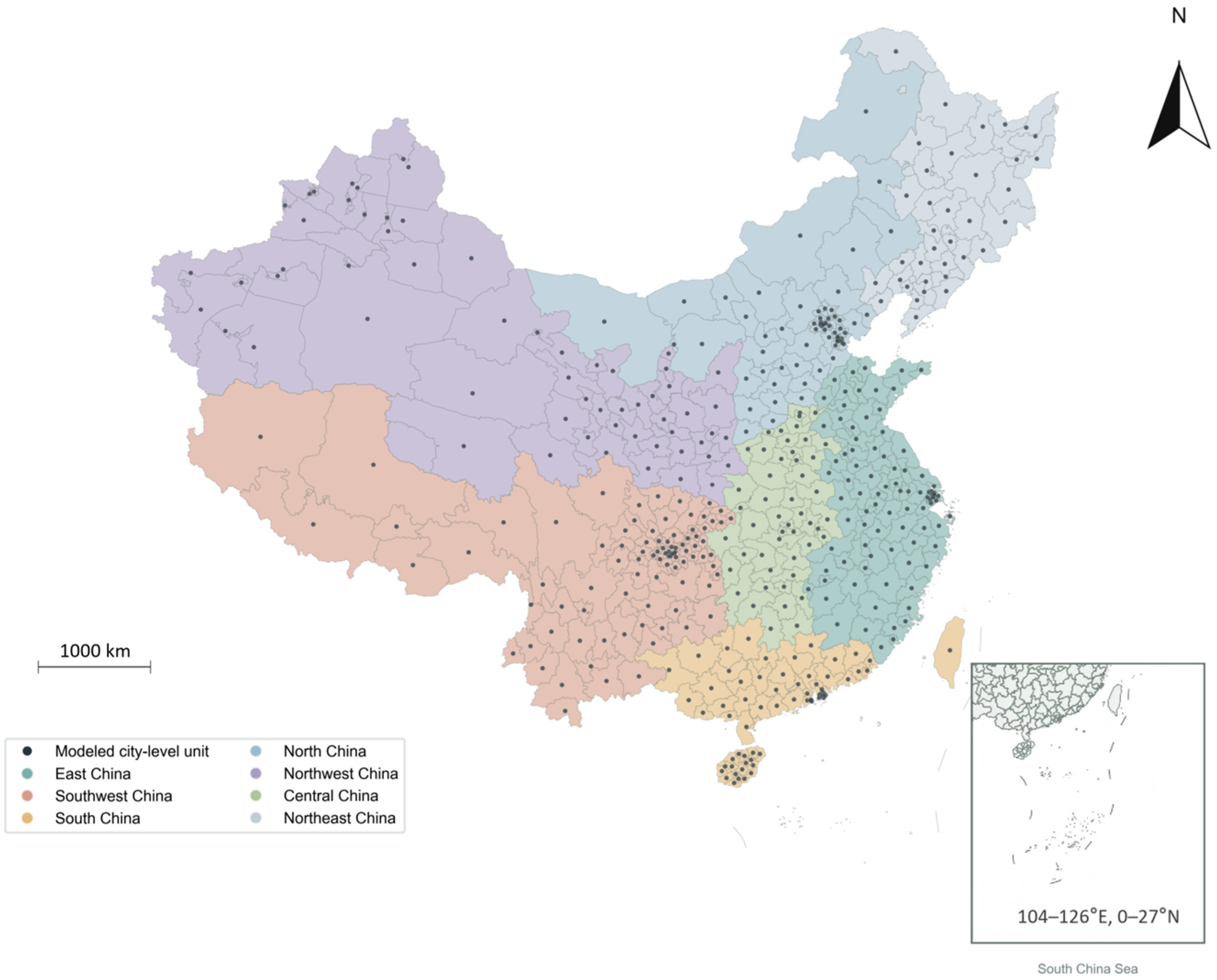
The spatial basis of the city-level panel is summarized in Figure 1. The figure shows the study area, the 475 city-level modeling units, the South China Sea inset, and the regional grouping used in subsequent spatial summaries. This spatial configuration provides the common reference for raster aggregation, meteorological matching, regional stratification, and the interpretation of later spatial error patterns.

2.2. Data Characteristics and Exploratory Diagnostics

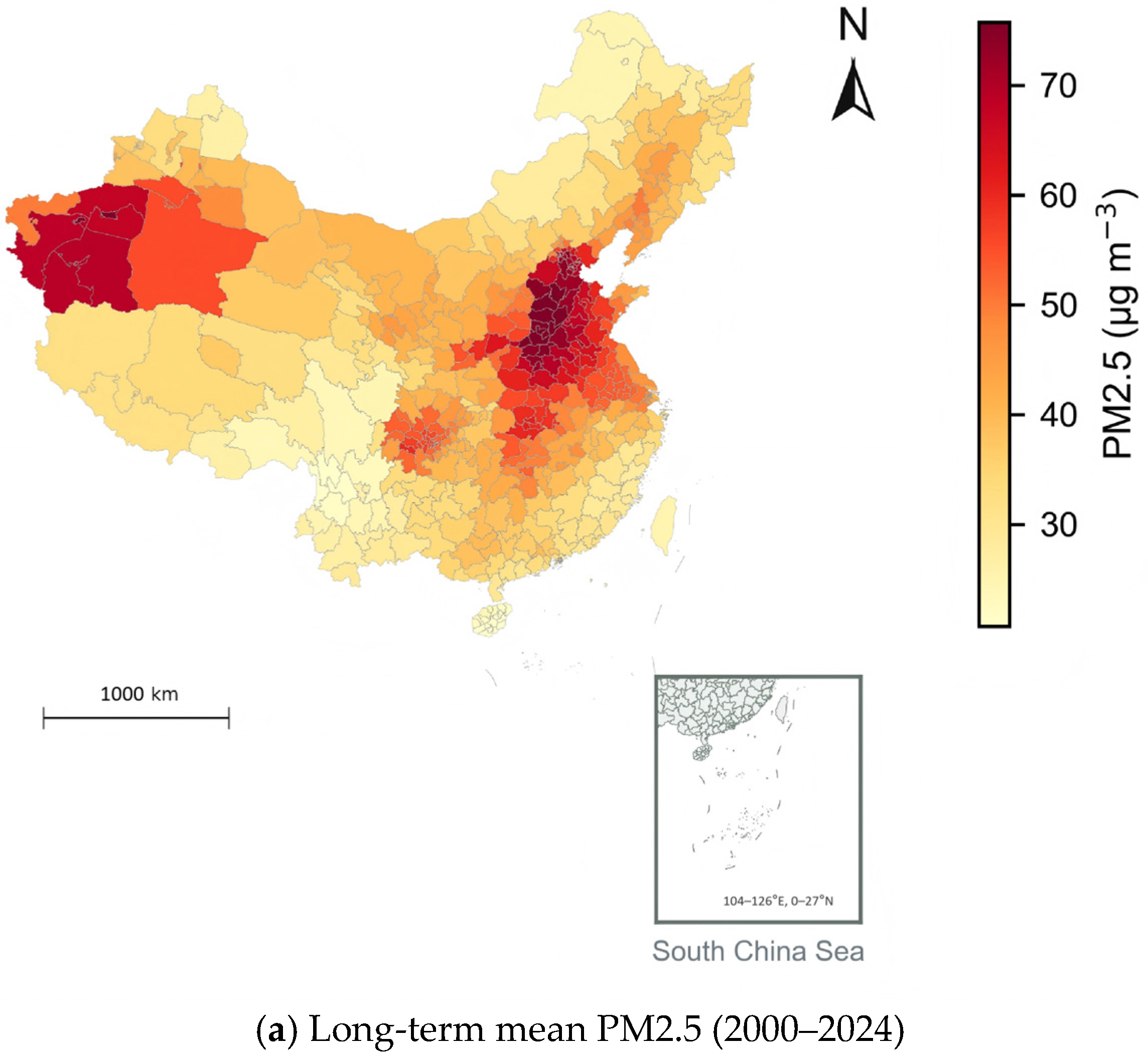
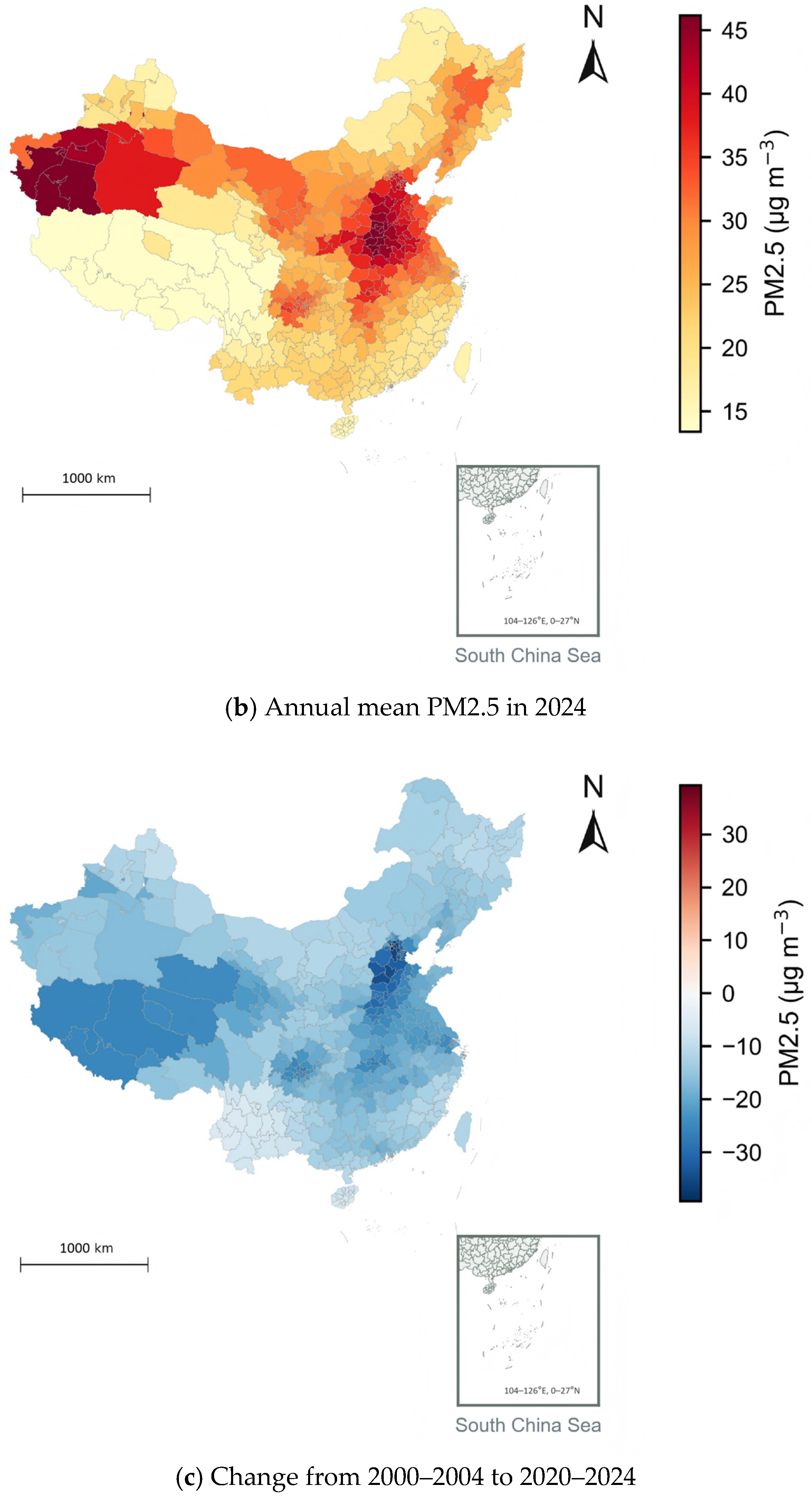
Based on the city-level monthly panel, Figure 2 extends the spatial overview from sample distribution to PM2.5 concentration patterns. Panel a depicts the long-term mean concentration during 2000–2024, representing the background pollution level for each city-level unit. Panel b maps the annual mean concentration in 2024 and therefore provides a recent-state reference. Panel c reports the change between the early stage—2000–2004—and the recent stage, 2020–2024, highlighting the direction and magnitude of long-term spatial change. Viewing these panels together helps distinguish persistent high-concentration areas, recent pollution levels, and regions with stronger historical reductions, which are subsequently useful for interpreting geographically heterogeneous prediction errors and model gains.

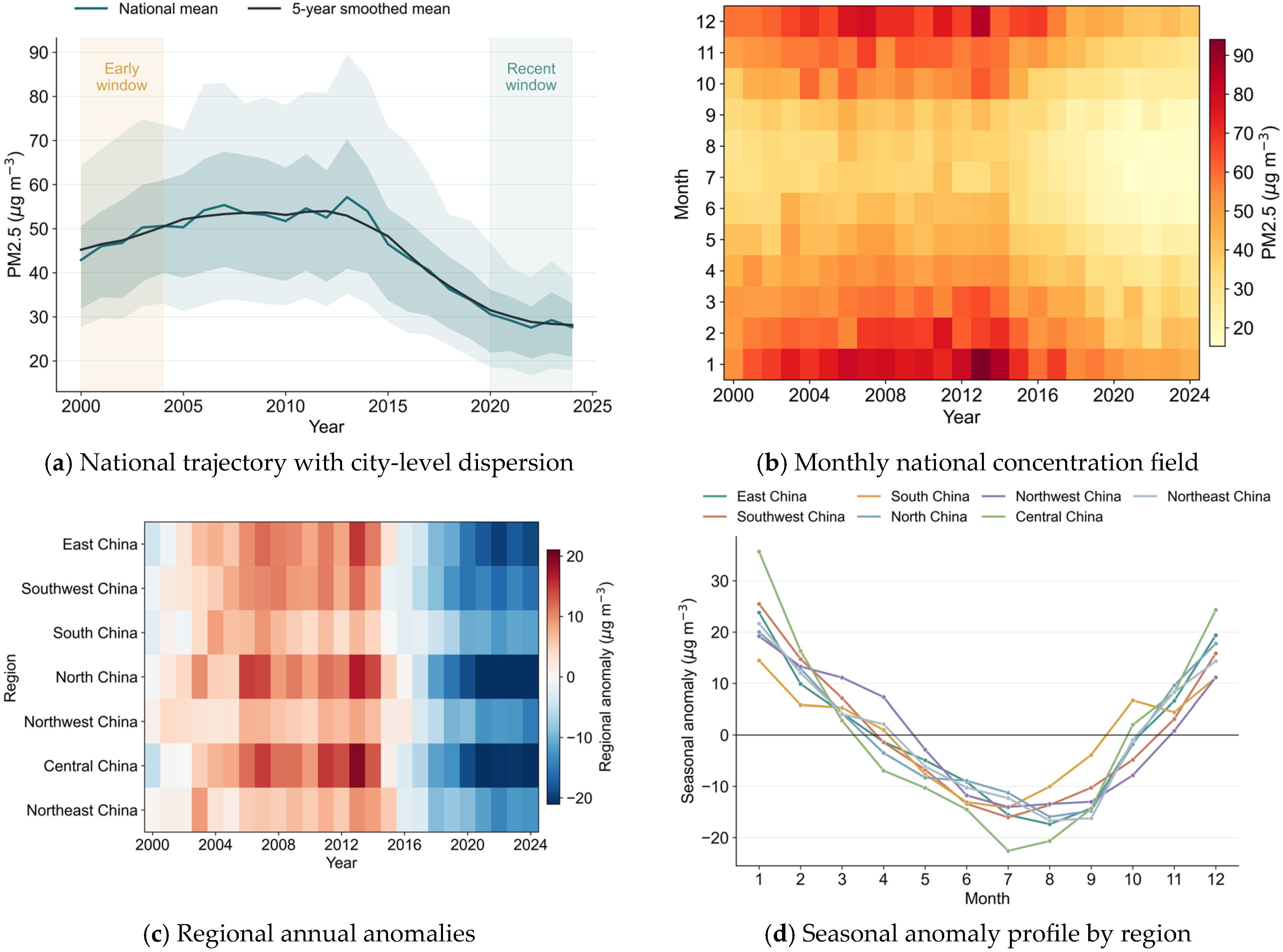
In the temporal dimension, Figure 3 characterizes the temporal structure of the PM2.5 panel before model construction. Panel a shows the national trajectory together with city-level dispersion, indicating the long-term evolution of the overall pollution background and the intercity variability around it. Panel b presents the month-by-year concentration field, making the seasonal alternation of high- and low-concentration periods visible over the full study period. Panel c compares regional annual anomalies, showing that temporal changes are not spatially uniform across the seven geographical regions. Panel d further displays the seasonal anomaly profiles by region, demonstrating broadly consistent winter enhancement and summer reduction but with region-specific amplitudes. These temporal and seasonal patterns motivate the use of sequence backbones and multi-scale decomposition features in the subsequent prediction framework.

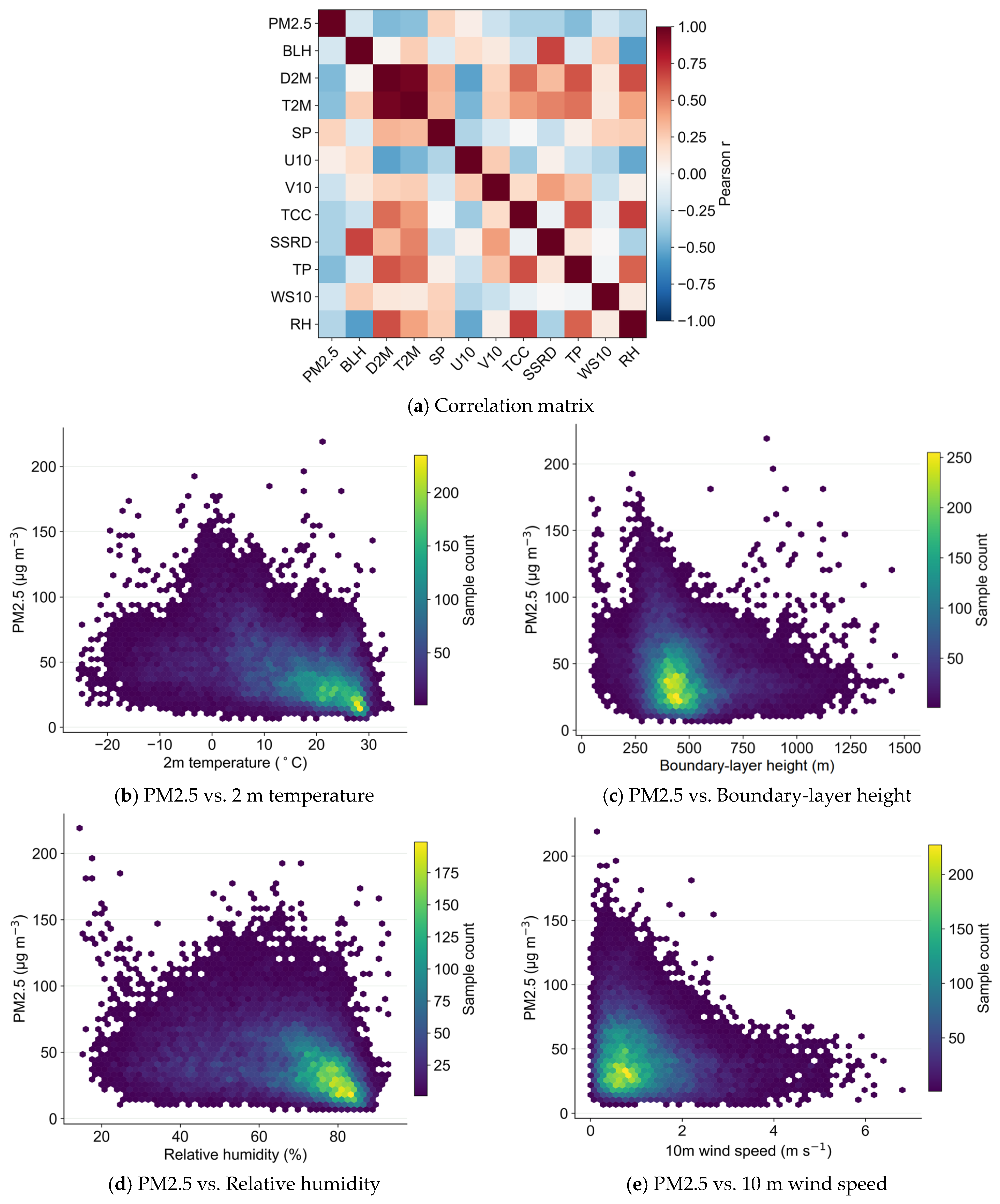
Before model construction, the statistical associations between PM2.5 and the meteorological covariates are examined in Figure 4. Panel a provides the correlation matrix among PM2.5 and the meteorological variables, giving an overview of linear dependence and potential collinearity. Panels b–e show representative bivariate relationships between PM2.5 and 2 m temperature, boundary-layer height, relative humidity, and 10 m wind speed using density-based scatter plots. The distributions indicate nonlinear and heterogeneous PM2.5–meteorology relationships, consistent with previously reported meteorological associations with particulate matter [39,40]. Relative humidity is retained as a predictive channel, whereas 10 m wind speed is shown here only as an exploratory diagnostic.

2.3. Spatial Aggregation and Data Preprocessing

Because the PM2.5 and ERA5 meteorological datasets differ in spatial resolution and spatial representation, this study applies differentiated spatial aggregation strategies. For the high-resolution PM2.5 raster data, valid grid cells falling within each city polygon are extracted according to administrative boundaries, and their regional mean is used as the monthly PM2.5 concentration for that city. For ERA5 meteorological data, the mean of grid points within each city polygon is calculated whenever possible; for cities without valid internal grid points, the nearest ERA5 grid point to the city centroid is used as a fallback match. Two derived meteorological variables are also retained in the city-month panel. Relative humidity is calculated from 2 m temperature and 2 m dewpoint temperature (both expressed in °C) as $\mathrm{rh}=100\exp \left[{\displaystyle \frac{17.67\hspace{0.17em}\mathrm{d}2\mathrm{m}}{243.5 + \mathrm{d}2\mathrm{m}}}-{\displaystyle \frac{17.67\hspace{0.17em}\mathrm{t}2\mathrm{m}}{243.5 + \mathrm{t}2\mathrm{m}}}\right]$, and the resulting relative humidity channel is retained in the final predictive tensor. The 10 m wind speed is calculated as $\mathrm{ws}10=\sqrt{\mathrm{u}{10}^2+\mathrm{v}{10}^2}$ and is used only for exploratory diagnostics; it is not supplied as an independent model-input channel. The 10 m u-component of wind and 10 m v-component of wind remain separate predictive channels.

During preprocessing, administrative division codes, city names, longitude, latitude, and dates are used for spatial aggregation, alignment, metadata, and indexing only; they are not supplied as predictive channels in the final 27-dimensional sequence tensor. Standardization parameters for the predictive features and target are fitted using the training set only and then reused for validation and test data. The added decomposition channels are standardized separately using means and standard deviations estimated from the training decomposition components only; the same statistics are then applied to the validation and test components.

Samples use a 12-month sequence to predict the following month. Because the engineered feature set includes a 12-month PM2.5 lag, the first valid forecast target is January 2002. Training input-end months span December 2001–November 2018 and correspond to targets January 2002–December 2018 (204 months); validation input-end months span December 2018–November 2021 and correspond to targets January 2019–December 2021 (36 months); test input-end months span December 2021–November 2024 and correspond to targets January 2022–December 2024 (36 months). The resulting tensors are (204, 475, 12, 27), (36, 475, 12, 27), and (36, 475, 12, 27), respectively. The city dimension is unfolded into city-month samples during training, while split assignment and standardization preserve temporal order.

Table 2. Exact predictive features in the final 27-dimensional sequence tensor.

Feature Group	Predictive Features (Tensor Code)	Number
ERA5 meteorological channels	Boundary-layer height (blh); 2 m temperature (t2 m); surface pressure (sp); 10 m u-component of wind (u10); 10 m v-component of wind (v10); total cloud cover (tcc); surface solar radiation downwards (ssrd); total precipitation (tp)	8
Derived meteorological channel	Relative humidity (rh)	1
Calendar encodings	Sine encoding of calendar month (month_sin); cosine encoding of calendar month (month_cos)	2
PM2.5 lag features	PM2.5 lag 1 month (pm25_lag1); PM2.5 lag 3 months (pm25_lag3); PM2.5 lag 6 months (pm25_lag6); PM2.5 lag 12 months (pm25_lag12)	4
Meteorological lag features	Boundary-layer height lag 1 month (blh_lag1); boundary-layer height lag 3 months (blh_lag3); total precipitation lag 1 month (tp_lag1); total precipitation lag 3 months (tp_lag3); relative humidity lag 1 month (rh_lag1); relative humidity lag 3 months (rh_lag3)	6
Rolling-mean features	PM2.5 3-month rolling mean (pm25_rollmean3); PM2.5 6-month rolling mean (pm25_rollmean6); PM2.5 12-month rolling mean (pm25_rollmean12); boundary-layer height 3-month rolling mean (blh_rollmean3); total precipitation 3-month rolling mean (tp_rollmean3); relative humidity 3-month rolling mean (rh_rollmean3)	6
Total	Final non-decomposition sequence tensor	27

lists the exact 27 channels supplied to the forecasting models. Eight channels are direct ERA5 meteorological variables, whereas relative humidity (rh) is a derived meteorological channel. The city-month panel also contains 2 m dewpoint temperature and derived 10 m wind speed. The former contributes to the construction of relative humidity, while the latter is used only for exploratory diagnostics; neither is supplied as an additional independent channel. Wind information in the predictive tensor is represented by the 10 m u-component of wind and 10 m v-component of wind.

2.4. Overall Forecasting Framework

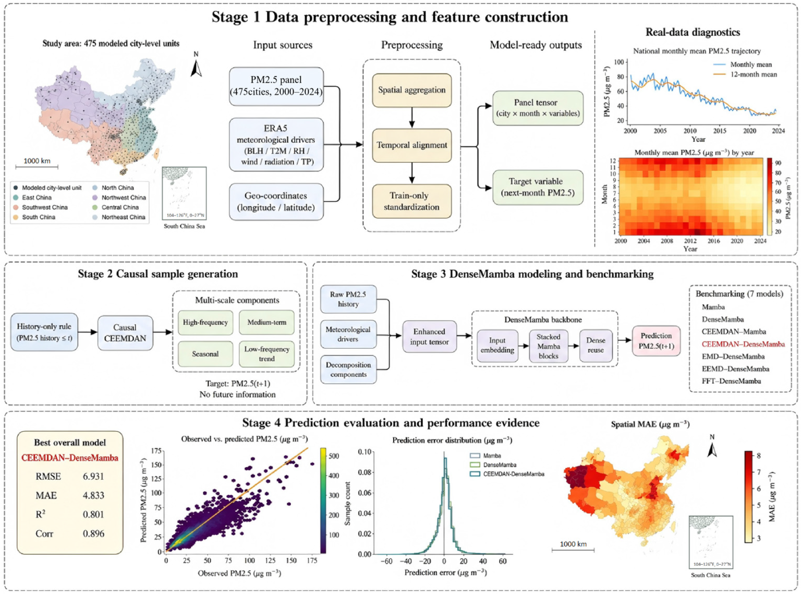
The proposed method is organized around temporally constrained multi-scale feature construction and Mamba-family temporal modeling. The comparison focuses on backbone architecture, history-only CEEMDAN feature construction, and alternative decomposition strategies within a structured experimental framework. Figure 5 outlines the workflow from multi-source data construction and temporally valid sample generation to enhanced feature formation, Mamba-family forecasting, and unified performance evaluation.

Under the framework shown in Figure 5, this study first integrates multi-source city-level observations into a unified monthly panel, constructs prediction samples under temporal constraints, and evaluates Mamba-family models with different backbone and decomposition-enhanced configurations under consistent data splits and metrics. The figure is intended to clarify the complete experimental logic rather than to imply a physical causal mechanism between individual components and PM2.5 concentration changes. Any “causal” wording retained inside the original schematic is used only in the restricted temporal sense of respecting information availability and does not denote physical or intervention-based causal inference.

The modeling pipeline consists of input construction, multi-scale feature construction, Mamba-family representation learning, and next-month PM2.5 prediction. For each sample, the 12-step non-decomposition input ends at month $t$ and the prediction target is month $t+1$. The final 27-dimensional tensor contains the engineered predictors listed in Table 2. The rolling decomposition routine uses PM2.5 values strictly preceding the input-end position, i.e., through month $t-1$, with at most 60 months of available history. The most recent 12 decomposition values are therefore concatenated as one-step-lagged multi-scale covariates with the 27-dimensional sequence features. With $K=4$, the enhanced input dimension is 31. The target month $t+1$ is never used during decomposition or feature construction.

Within this framework, Mamba and DenseMamba serve as non-decomposition baselines, providing references for cases without additional multi-scale decomposition features. The CEEMDAN-enhanced variants are paired with the two backbone structures to distinguish decomposition-enhanced inputs from backbone-level changes. EMD-DenseMamba, EEMD-DenseMamba, and FFT-DenseMamba are constructed as alternative-decomposition comparison models to determine whether the advantage of CEEMDAN arises from its specific decomposition mechanism or merely from a general expansion of multi-scale features.

This comparison design clarifies the intended contrasts and their boundaries. All seven formal models use the same chronological split, evaluation metrics, repeated-seed protocol, and test-set assessment procedure. The four decomposition-enhanced DenseMamba variants additionally share identical backbone architecture and training hyperparameters, whereas Mamba, DenseMamba, and CEEMDAN-Mamba use pre-specified model-specific configurations disclosed in Section 2.8. Because those structural pairs are not optimization-identical in the primary benchmark, architecture-level effects are examined separately under one common optimization configuration.

2.5. Temporally Constrained Rolling Multi-Scale Decomposition and Leakage Control

PM2.5 series exhibit strong non-stationarity and multi-scale variability, with different frequency components potentially corresponding to long-term trends, seasonal cycles, short-term fluctuations, and local abnormal disturbances. When the raw sequence is modeled directly, the model must simultaneously handle multiple heterogeneous dynamics, increasing the learning difficulty. CEEMDAN adaptively decomposes a complex signal into several intrinsic mode functions (IMFs) while preserving local variations in non-stationary sequences and reducing mode mixing [22,23]. In this study, CEEMDAN is restricted to rolling historical windows to ensure that each sample’s decomposition features are constructed only from information available up to the prediction time.

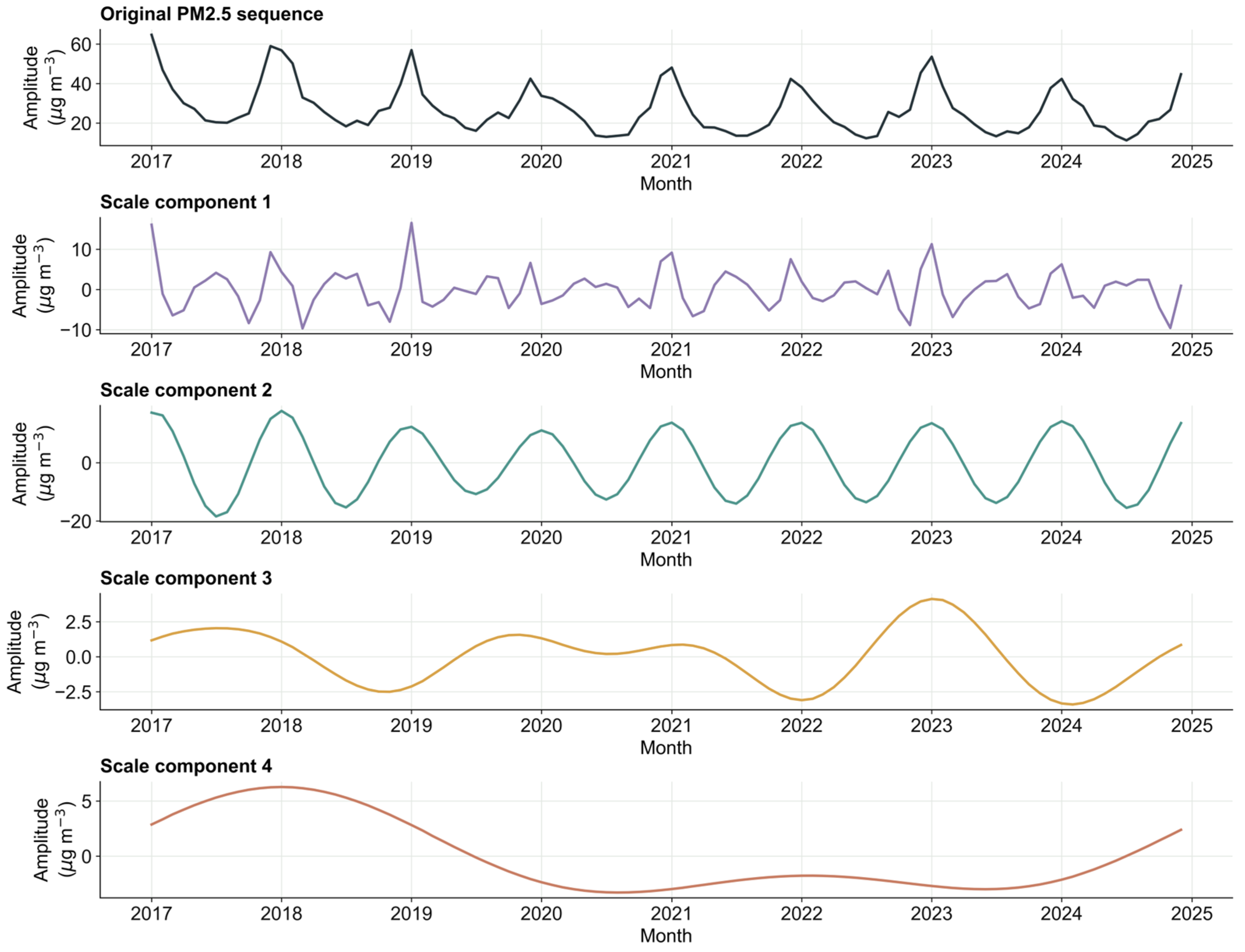
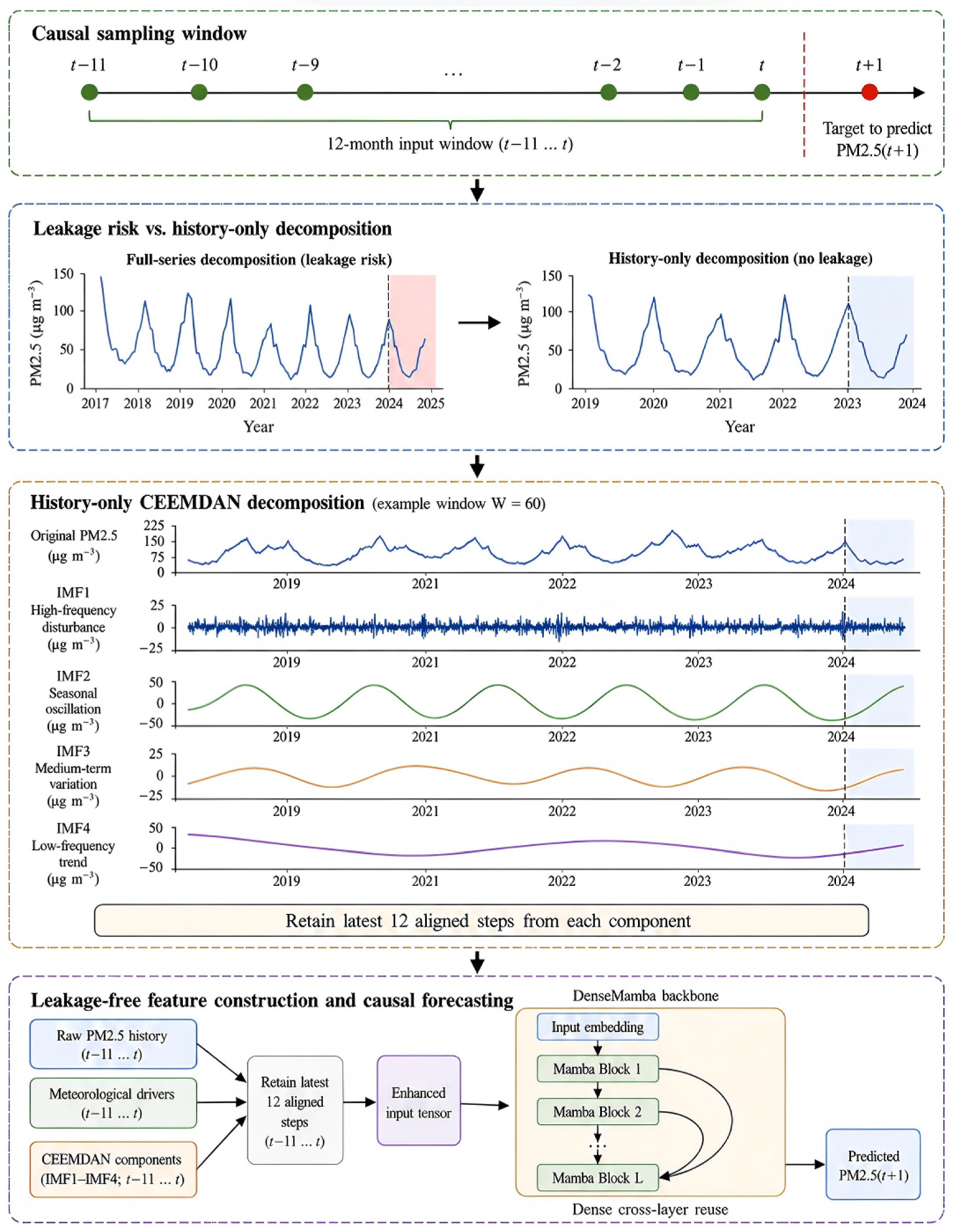
Figure 6 illustrates temporally constrained rolling decomposition and leakage-free multi-scale feature construction. If a full series is decomposed before the training, validation, and test sets are separated, features for earlier samples can depend on later observations. In contrast, the implementation used here rebuilds the decomposition input for every city-month sample using only PM2.5 values preceding the sample-specific cutoff. The latest 12 component values are then used as one-step-lagged multi-scale covariates alongside the 27-dimensional predictive tensor. Any “causal” label retained inside Figure 6 refers only to this temporal information constraint.

The top time series shows the PM2.5 reference sequence, while the component curves illustrate variation at different temporal scales. The retained component values are truncated to the latest 12 values available before the input-end month and are used as one-step-lagged multi-scale predictors. The components are treated as algorithmic features rather than physically invariant modes, so their role is to make multi-scale information inspectable without using future observations.

Let $x_{c,t}$ denote the ChinaHighPM2.5 reference value for city $c$ at month $t$. For a sample whose model input ends at $t$, the forecast target is $t+1$. Let $L=12$ be the input length, let $A_{c,t}$ denote the number of PM2.5 months available before $t$, and define the effective decomposition-window length as $W_{c,t}=\min \left(60,A_{c,t}\right)$. No padding or repeated observations are introduced when fewer than 60 preceding months are available. The history-only window is

$$H_{c,t}^{W_{c,t}}=\left\{x_{c,t-W_{c,t}},\dots ,x_{c,t-1}\right\}, W_{c,t}\ge L.$$

(1)

For the earliest training input-end month, December 2001, $A_{c,t}=23$; this is the only forecast origin per city with fewer than 24 preceding months and therefore uses the pre-specified FFT fallback. From the following training month onward, CEEMDAN is used whenever at least 24 preceding months are available. In every case, decomposition stops at $t-1$, while the forecast target remains $t+1$.

For CEEMDAN, EMD, and EEMD, let $d$ index the decomposition method and let $J_{c,t}^{\left(d\right)}$ be the number of components returned from the history-only window. The decomposition output and reconstruction are written as:

$${\mathcal{D}}_d\left(H_{c,t}^{W_{c,t}}\right)=\left\{u_{c,t,1}^{\left(d\right)},\dots ,u_{c,t,J_{c,t}^{\left(d\right)}}^{\left(d\right)},r_{c,t}^{\left(d\right)}\right\}, H_{c,t}^{W_{c,t}}={\displaystyle {\displaystyle \sum }_{j=1}^{J_{c,t}^{\left(d\right)}}}{u}_{c,t,j}^{\left(d\right)}+r_{c,t}^{\left(d\right)}.$$

(2)

Here, $u_{c,t,j}^{\left(d\right)}$ is the $j$th returned component and $r_{c,t}^{\left(d\right)}$ is the residual. The forecasting input retains $K=4$ component channels: if $J_{c,t}^{\left(d\right)}<K$, missing channels are zero-padded; if $J_{c,t}^{\left(d\right)}>K$, only the first $K$ components are retained. The residual is not concatenated with the predictors. FFT components are defined separately and are not referred to as IMFs. Figure 7 provides an illustrative example of the CEEMDAN multi-scale decomposition of a representative PM2.5 sequence.

$$X_{c,t}^{\left(d\right)}=\mathrm{Concat}\left[X_{c,t}^{\mathrm{raw}},{\mathrm{Last}}_L\left(u_{c,t,1}^{\left(d\right)},\dots ,u_{c,t,K}^{\left(d\right)}\right)\right].$$

(3)

Let $X_{c,t}^{\mathrm{raw}}\in {ℝ}^{L\times 27}$ denote the non-decomposition input and $X_{c,t}^{\mathrm{enh}}\in {ℝ}^{L\times \left(27+K\right)}$ the enhanced input. For EMD-family methods, the additional channels are the retained components defined above; for FFT, they are the frequency-mask reconstructions defined below. All component values are computed from PM2.5 preceding $t$ and are therefore one-step lagged relative to the final raw-input month. With $L=12$ and $K=4$, $X_{c,t}^{\mathrm{enh}}\in {ℝ}^{12\times 31}$.

Table 3. Exact temporal split and decomposition coverage.

Data Split	Target Period	Forecast Months	City-Time Paired Samples	CEEMDAN Samples	FFT Fallback Samples	CEEMDAN Coverage (%)
Training set	January 2002–December 2018	204	96,900	96,425	475	99.510
Validation set	January 2019–December 2021	36	17,100	17,100	0	100.000
Test set	January 2022–December 2024	36	17,100	17,100	0	100.000

combines the exact target periods with decomposition coverage. The 475 FFT fallback cases correspond exactly to one earliest training forecast month for each of the 475 cities (0.490% of the training city-month pairs). No validation or test sample uses the fallback; both sets have 100% CEEMDAN coverage. The fallback therefore affects only a small early-history portion of training. It preserves the same four-channel tensor layout as the decomposition-enhanced inputs, while no validation or test sample undergoes a CEEMDAN-to-FFT feature shift.

CEEMDAN functions as a multi-scale feature-construction module rather than a standalone predictor. The primary benchmark pre-specifies $K=4$ retained components to keep the enhanced input dimension fixed. If fewer than four modes are returned, missing channels are zero-padded; if more than four are returned, only the first four are retained. The residual is not supplied as an additional input feature. IMF order is treated as an algorithmic feature position rather than a physically invariant frequency band across rolling windows, because modal content can shift when the historical window changes. Accordingly, the decomposition channels are interpreted as inspectable predictive representations rather than direct physical explanations.

The decomposition procedures were implemented using EMD-signal version 1.10.0 (imported as PyEMD). CEEMDAN is instantiated as CEEMDAN (trials = 50, parallel = False), EEMD uses 50 trials, and EMD uses the library implementation without additional manually specified parameters. The implementation uses a base decomposition seed of 2024 to construct a deterministic city-specific NumPy RandomState and resets NumPy’s global random state before each rolling-window call. No library-specific noise-seed method is invoked. Noise amplitude, stopping thresholds, and other decomposition settings are not manually overridden and therefore follow the library defaults. Unlike one-time full-series decomposition, a history window is rebuilt for each sample. The same cached decomposition components were retained in the additional controlled analyses to maintain consistency with the primary benchmark.

For FFT-DenseMamba and the early-history fallback, the available PM2.5 history is transformed in the frequency domain and reconstructed through fixed masks. Let $x=\left(x_0,\dots ,x_{N_h-1}\right)$ be an $N_h$-point history and let $f_k$ denote the normalized frequencies returned by numpy.fft.fftfreq. The discrete Fourier coefficients and the $m$th masked reconstruction are

$${\widehat{x}}_k={\displaystyle {\displaystyle \sum }_{n=0}^{N_h-1}}{x}_n\exp \left(-{\displaystyle \frac{2\pi ikn}{N_h}}\right), u_m^{\mathrm{FFT}}=\mathrm{Re}\left\{\mathrm{IFFT}\left(\widehat{x}\odot M_m\right)\right\}.$$

(4)

For $m=1,\dots ,K-1$, the implemented mask retains frequencies satisfying $0.5/2^m\le \left|f_k\right|<0.5/2^{m-1}$. The final mask retains $\left|f_k\right|<0.5/2^{\max \left(1,K-2\right)}$. With $K=4$, the final low-frequency mask overlaps the third band over $0.0625\le \left|f_k\right|<0.125$. The FFT channels are therefore fixed frequency-mask reconstructions, not an orthogonal partition and not IMFs; no reconstruction identity analogous to Equation (2) is assumed.

2.6. Mamba and DenseMamba Backbones

At the sequence-modeling stage, Mamba and DenseMamba are used as the core Mamba-inspired backbones. The implementation is a custom lightweight selective state-space block tailored to this forecasting task rather than a direct call to the official Mamba-ssm library. It contains input projection, depthwise causal convolution, selective state update, gated fusion, residual connection, and dropout. The model-input length $L=12$ is chosen to provide one complete annual cycle at monthly resolution; this setting is task-specific and is not used as evidence of a long-sequence advantage. The architecture constants $D=128$, $N_{\mathcal{l}}=4$, $N_s=16$, and $d_{\mathrm{conv}}=4$ correspond to the implementation settings D_MODEL, N_LAYERS, D_STATE, and D_CONV, respectively. They were fixed a priori for all Mamba-family variants and were not tuned through a dedicated architecture search or selected using the test set. The selective state update can be abstracted as

$$H_{\mathcal{l},\tau }=\exp \left[A_{\mathcal{l}}\odot \left({\Delta }_{\mathcal{l},\tau }{\mathbf{1}}_{N_s}^{\top }\right)\right]\odot H_{\mathcal{l},\tau -1}+\left({\Delta }_{\mathcal{l},\tau }\odot x_{\mathcal{l},\tau }\right)B_{\mathcal{l},\tau }^{\top }, o_{\mathcal{l},\tau }=H_{\mathcal{l},\tau }{C}_{\mathcal{l},\tau }.$$

(5)

For sequence position $\tau$ in layer $\mathcal{l}$, $x_{\mathcal{l},\tau }, {\Delta }_{\mathcal{l},\tau }\in {ℝ}^D$, $B_{\mathcal{l},\tau },C_{\mathcal{l},\tau }\in {ℝ}^{N_s}$, and $A_{\mathcal{l}},H_{\mathcal{l},\tau }\in {ℝ}^{D\times N_s}$, with $D=128$ and $N_s=16$. The code parameterizes $A_{\mathcal{l}}=-\exp \left(A_{\log ,\mathcal{l}}\right)$ and ${\Delta }_{\mathcal{l},\tau }=\mathrm{softplus}\left(W_{\Delta }{x}_{\mathcal{l},\tau }+b_{\Delta }\right)$, so $A_{\mathcal{l}}<0$ and ${\Delta }_{\mathcal{l},\tau }>0$. The exponential in Equation (5) is element-wise, giving transition factors in $\left(0,1\right)$. Multiplication by $C_{\mathcal{l},\tau }$ reduces the state dimension and returns a $D$-dimensional output. The surrounding block then applies SiLU-gated fusion, output projection, dropout, and a residual connection. Here, $x_{\mathcal{l},\tau }$ denotes the SelectiveSSM input after the depthwise causal convolution and sigmoid linear unit (SiLU) activation; $W_{\Delta }\in {ℝ}^{D\times D}$ and $b_{\Delta }\in {ℝ}^D$.

First, the input sequence is mapped into a unified hidden space through a linear layer, LayerNorm, and Gaussian error linear unit (GELU), producing the initial representation

$$Z_0=E\left(X_{c,t}\right).$$

(6)

where $E\left(\cdot \right)$ denotes the input-embedding module composed of linear mapping, LayerNorm, and GELU. To enhance information flow and feature reuse in deeper sequence models, dense connections are introduced between Mamba layers. The idea of dense connections originates from DenseNet, whose central advantage is promoting feature reuse and alleviating information attenuation in deep networks [27].

$$G_{\mathcal{l}}=\mathrm{Concat}\left[Z_0,Z_1,\dots ,Z_{\mathcal{l}-1}\right].$$

(7)

For DenseMamba, the input to the $\mathcal{l}$th layer is formed by concatenating all previous layer representations and then compressing them back to the unified hidden dimension. In the code, this fusion is implemented as a Concat–Linear–LayerNorm–GELU operation:

$$Z_{\mathcal{l}}^{\ast }=F_{\mathcal{l}}\left(G_{\mathcal{l}}\right).$$

(8)

The fused representation is then fed into the $\mathcal{l}$th MambaBlock to obtain the output representation of the current layer:

$$Z_{\mathcal{l}}={\mathrm{MambaBlock}}_{\mathcal{l}}\left(Z_{\mathcal{l}}^{\ast }\right), \mathcal{l}=1,\dots ,N_{\mathcal{l}}.$$

(9)

The overall model structure can be summarized as four stages: input construction, hidden-space embedding, Mamba-family encoding, and prediction output. In the Mamba model, the input sequence is embedded and then passed sequentially through MambaBlocks for state-space encoding. In the DenseMamba model, dense feature reuse is additionally introduced across layers. For decomposition-enhanced models, the front-end decomposition module expands the input with multi-scale dynamic features; for non-decomposition models, the backbone directly models the 27-dimensional non-decomposition feature tensor. This study does not interpret the relationship between decomposition modules and predictive performance as a fully established physical causal mechanism; instead, it observes relative error differences among backbones and decomposition methods under unified evaluation rules.

Here, $\mathrm{Concat}\left(\cdot \right)$ denotes concatenation along the feature dimension, $F_{\mathcal{l}}\left(\cdot \right)$ denotes the feature-fusion mapping at layer $\mathcal{l}$, and $N_{\mathcal{l}}$ denotes the number of stacked MambaBlock layers. In the code, $D=128$, $N_{\mathcal{l}}=4$, $N_s=16$, $d_{\mathrm{conv}}=4$, and dropout is 0.2. The fusion operation is Concat-Linear-LayerNorm-GELU rather than gated dense fusion. This design keeps earlier layer representations accessible to later blocks; its effect on forecast error is assessed empirically under matched optimization.

2.7. Controlled Model Comparison Design

The primary benchmark comprises seven formal models. Mamba and DenseMamba are non-decomposition baselines; CEEMDAN-Mamba and CEEMDAN-DenseMamba provide CEEMDAN-enhanced counterparts; and EMD-DenseMamba, EEMD-DenseMamba, and FFT-DenseMamba compare alternative decomposition front ends under an identical DenseMamba backbone and training configuration. The chronological split and evaluation protocol are common to all seven models, but the structural Mamba/DenseMamba pairs use pre-specified model-specific optimization settings. Their architecture-level effects are therefore interpreted descriptively in the primary benchmark and examined separately under equal optimization.

CEEMDAN-Mamba and CEEMDAN-DenseMamba use CEEMDAN to construct IMFs. EMD-DenseMamba uses EMD, EEMD-DenseMamba uses EEMD, and FFT-DenseMamba uses the frequency-mask construction defined in Section 2.5. All decomposition-enhanced models follow the same history-only window and input-concatenation procedure. The four decomposition-enhanced DenseMamba variants share identical backbone and optimization settings and therefore provide the cleanest matched comparison of decomposition front ends.

Let ${\mathcal{D}}_d\left(\cdot \right)$ denote the decomposition operator corresponding to decomposition method $d$, where $d\in \left\{\mathrm{CEEMDAN},\mathrm{EMD},\mathrm{EEMD},\mathrm{FFT}\right\}$. The unified multi-scale input can be written as:

$$X_{c,t}^{\left(d\right)}=\mathrm{Concat}\left[X_{c,t}^{\mathrm{raw}},{\mathrm{Last}}_L\left({\mathrm{First}}_K\left({\mathcal{D}}_d\left(H_{c,t}^{W_{c,t}}\right)\right)\right)\right].$$

(10)

Here, ${\mathcal{D}}_d$ denotes the method-specific component extractor after CEEMDAN, EMD, EEMD, and FFT have been defined separately. ${\mathrm{First}}_K\left(\cdot \right)$ retains the first $K$ component channels, whereas ${\mathrm{Last}}_L\left(\cdot \right)$ selects the latest $L$ values available before the input-end month. The primary benchmark fixes $K=4$ and $L=12$ to maintain a common enhanced input shape. The notation unifies the model input but does not imply that FFT satisfies the EMD-family reconstruction relation in Equation (2).

2.8. Training Configuration and Evaluation Metrics

Training minimizes mean squared error (MSE) on the standardized target. Let ${\tilde{y}}_m$ and ${\widehat{\tilde{y}}}_m$ denote the standardized reference target and model output for sample $m=1,\dots ,M$, respectively, where $M$ denotes the number of samples included in the loss calculation. The training loss is

$${\mathrm{MSE}}_{\mathrm{train}}={\displaystyle \frac{1}{M}}{\displaystyle {\displaystyle \sum }_{m=1}^M}{\left({\tilde{y}}_m-{\widehat{\tilde{y}}}_m\right)}^2.$$

(11)

Model optimization uses AdamW [41,42] with ReduceLROnPlateau scheduling, gradient clipping, and early stopping. Each formal model is repeated with random seeds 42, 52, and 62 and summarized as mean ± standard deviation. Automatic hyperparameter tuning is disabled in the formal benchmark, and the test set is reserved for final reporting after validation-based model selection.

Table 4. Training configurations and trainable parameter counts of the primary seven-model benchmark.

Model	Input Dim.	Learning Rate	Weight Decay	Scheduler Patience	Early-Stop Patience	Min. Epochs	Trainable Parameters
Mamba	27	2 × 10−4	1 × 10−5	8	28	20	369,281
DenseMamba	27	1.5 × 10−4	5 × 10−6	10	35	30	534,657
CEEMDAN-Mamba	31	2 × 10−4	1 × 10−5	8	32	24	369,793
CEEMDAN-DenseMamba	31	1 × 10−4	5 × 10−6	10	40	32	535,169
EMD-DenseMamba	31	1 × 10−4	5 × 10−6	10	40	32	535,169
EEMD-DenseMamba	31	1 × 10−4	5 × 10−6	10	40	32	535,169
FFT-DenseMamba	31	1 × 10−4	5 × 10−6	10	40	32	535,169

discloses the model-specific optimization settings and trainable parameter counts used in the primary seven-model benchmark. The four decomposition-enhanced DenseMamba variants share identical optimization and architecture settings; the remaining structural variants use the pre-specified configurations shown in Table 4. To separate architecture from optimization more directly, a separate equal-optimization analysis retrains Mamba, DenseMamba, CEEMDAN-Mamba, and CEEMDAN-DenseMamba with the same training configuration.

For all formal models, the maximum epoch budget is 120, batch size is 128, gradient clipping is 5.0, dropout is 0.2, and feature masking is disabled. The remaining optimizer and early-stopping settings are model-specific and are reported explicitly in Table 4. This disclosure is used to separate the primary benchmark from the equal-optimization attribution experiment rather than to imply that all seven formal models were trained with identical hyperparameters. The experiments were implemented using PyTorch version 2.13.0 and scikit-learn version 1.9.0 [43,44].

After inverse transformation to the original PM2.5 scale, let $y_m$ and ${\widehat{y}}_m$ denote the reference target and prediction for sample $m=1,\dots ,M$, respectively, where $M$ is the number of evaluated samples. Evaluation metrics include root mean squared error (RMSE), mean absolute error (MAE), the coefficient of determination ($R^2$), mean absolute percentage error (MAPE), and the correlation coefficient (Corr). RMSE measures overall error magnitude and is more sensitive to large errors; MAE reflects mean absolute deviation; $R^2$ summarizes explained variation in the reference target; MAPE expresses absolute error relative to the reference target; and Corr measures linear agreement between predictions and reference targets. To avoid instability near zero, MAPE is computed only for samples satisfying $\left|y_m\right|>{10}^{-6}$ and is reported as a percentage. The metrics are defined in Equations (12)–(16).

$$\mathrm{RMSE}=\sqrt{{\displaystyle \frac{1}{M}}{\displaystyle {\displaystyle \sum }_{m=1}^M}{\left(y_m-{\widehat{y}}_m\right)}^2}.$$

(12)

$$\mathrm{MAE}={\displaystyle \frac{1}{M}}{\displaystyle {\displaystyle \sum }_{m=1}^M}\left|y_m-{\widehat{y}}_m\right|.$$

(13)

$$R^2=1-{\displaystyle \frac{{\sum }_{m=1}^M{\left(y_m-{\widehat{y}}_m\right)}^2}{{\sum }_{m=1}^M{\left(y_m-\overline{y}\right)}^2}}.$$

(14)

$$\mathrm{Corr}={\displaystyle \frac{{\sum }_{m=1}^M\left(y_m-\overline{y}\right)\left({\widehat{y}}_m-\overline{\widehat{y}}\right)}{\sqrt{{\sum }_{m=1}^M{\left(y_m-\overline{y}\right)}^2{\sum }_{m=1}^M{\left({\widehat{y}}_m-\overline{\widehat{y}}\right)}^2}}}.$$

(15)

$$\mathrm{MAPE}={\displaystyle \frac{100}{\left|{\mathcal{I}}_{\epsilon }\right|}}{\displaystyle \sum }_{m\in {\mathcal{I}}_{\epsilon }}{\displaystyle \frac{\left|y_m-{\widehat{y}}_m\right|}{\left|y_m\right|}}, {\mathcal{I}}_{\epsilon }=\left\{m:\left|y_m\right|>{10}^{-6}\right\}.$$

(16)

Here, $\overline{y}$ and $\overline{\widehat{y}}$ are the sample means. The set ${\mathcal{I}}_{\epsilon }$ in Equation (16) implements the threshold $\left|y_m\right|>{10}^{-6}$. Corr is evaluated by Equation (15) when both vectors have nonzero variance; otherwise the implementation returns 0.

3. Results

3.1. Overall Predictive Performance of the Seven Models

The primary seven-model benchmark compares Mamba, DenseMamba, CEEMDAN-Mamba, CEEMDAN-DenseMamba, EMD-DenseMamba, EEMD-DenseMamba, and FFT-DenseMamba on the common chronological test set (

Table 5. Test-set performance of the seven formal models.

Model Variant	Input Type	RMSE	MAE	${\mathit{R}}^{\mathbf{2}}$	MAPE (%)	Corr
Mamba	Non-decomposition	7.280 ± 0.153	5.298 ± 0.149	0.781 ± 0.009	20.928 ± 1.143	0.887 ± 0.006
DenseMamba	Non-decomposition	7.311 ± 0.275	5.304 ± 0.279	0.779 ± 0.017	21.070 ± 1.950	0.887 ± 0.007
CEEMDAN- Mamba	CEEMDAN- enhanced	6.942 ± 0.205	4.917 ± 0.186	0.800 ± 0.012	18.850 ± 0.922	0.896 ± 0.006
CEEMDAN- DenseMamba	CEEMDAN- enhanced	6.931 ± 0.047	4.833 ± 0.066	0.801 ± 0.003	18.084 ± 0.524	0.896 ± 0.002
EMD- DenseMamba	EMD- enhanced	7.060 ± 0.131	4.936 ± 0.123	0.794 ± 0.008	18.681 ± 0.822	0.893 ± 0.004
EEMD- DenseMamba	EEMD- enhanced	7.316 ± 0.210	5.186 ± 0.433	0.778 ± 0.013	20.092 ± 3.472	0.887 ± 0.003
FFT- DenseMamba	FFT- enhanced	7.018 ± 0.175	4.969 ± 0.285	0.796 ± 0.010	18.692 ± 2.401	0.894 ± 0.005

and Figure 8). Mamba and DenseMamba use the 27-dimensional non-decomposition input; the remaining models add temporally constrained multi-scale components. The formal repeated-seed protocol and model-specific training configurations are described in Section 2.8 and Table 4. Results are reported as mean ± standard deviation across seeds 42, 52, and 62.

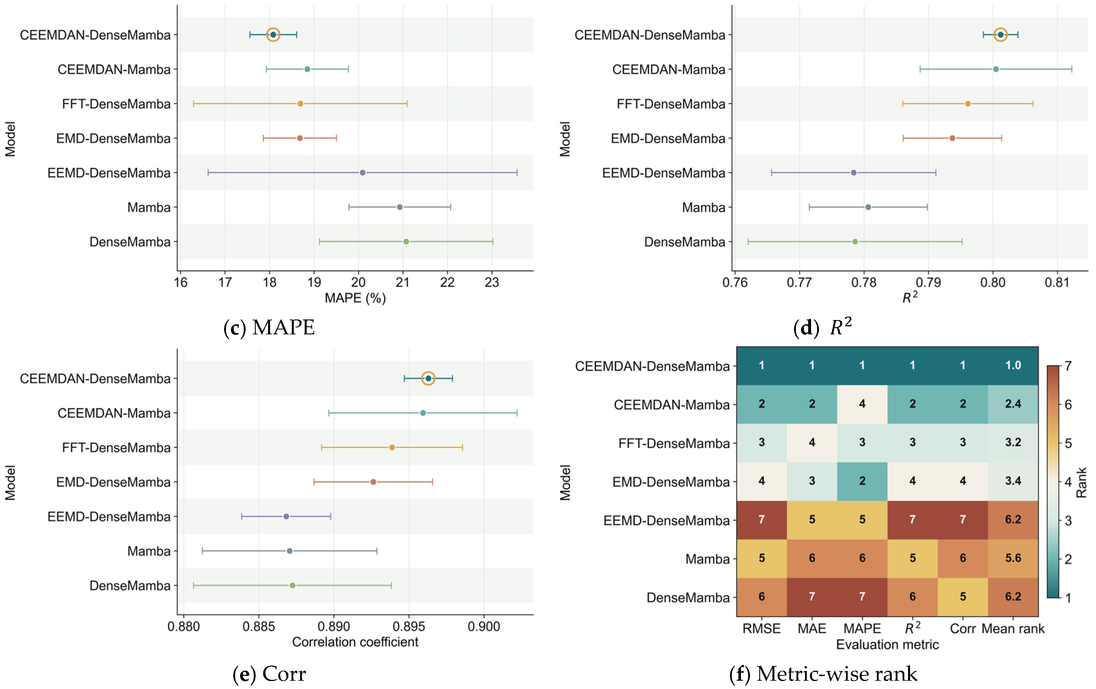
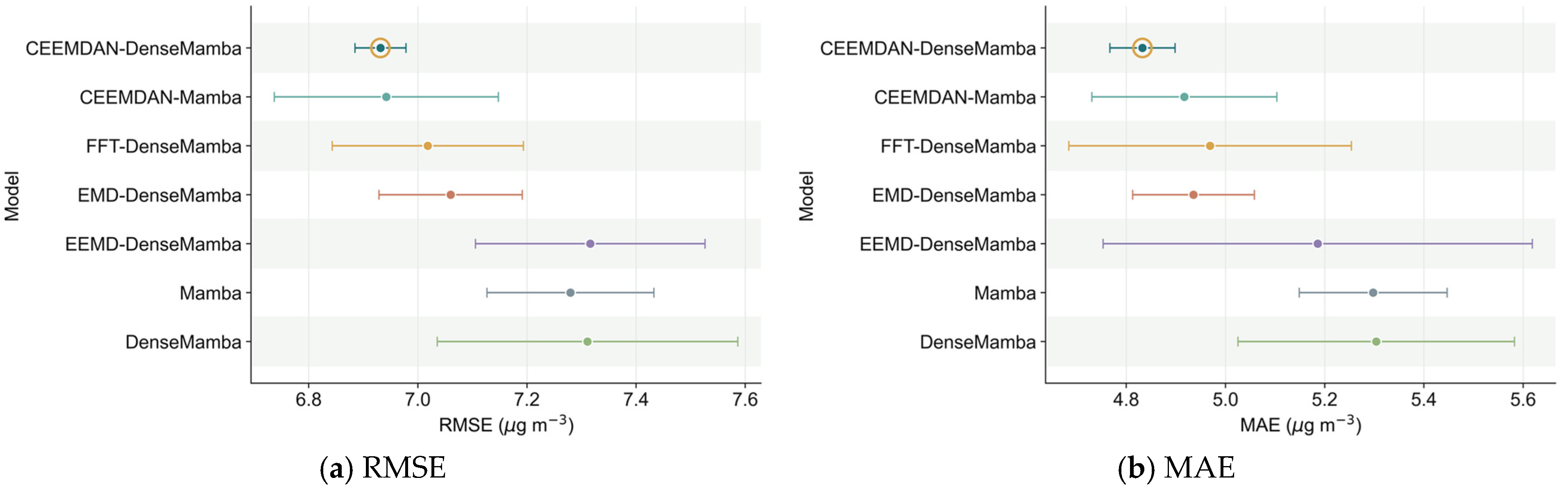
The multi-metric comparison in Figure 8 evaluates the seven formal models from both error-oriented and agreement-oriented perspectives. Panels a–c compare error-oriented metrics—namely, root mean squared error, mean absolute error, and mean absolute percentage error—where lower values indicate better predictive accuracy. Panels d and e compare the coefficient of determination and the correlation coefficient, where higher values indicate stronger agreement with the reference targets. Panel f summarizes the metric-wise rankings across all five metrics, providing an integrated view of model performance. In the ranking matrix, a smaller rank denotes better performance, with rank 1 indicating the best model for a given metric. Across these complementary diagnostics, CEEMDAN-DenseMamba achieves the most favorable overall trade-off among error reduction, agreement, and cross-seed stability.

Numerically, CEEMDAN-DenseMamba has the lowest mean RMSE and MAE in the primary seven-model benchmark, with values of 6.931 and 4.833 μg m⁻³, respectively. These benchmark rankings are descriptive because the structural Mamba/DenseMamba pairs use different pre-specified optimization settings. Accordingly, Table 5 is interpreted descriptively; dense connectivity and the incremental CEEMDAN contribution are evaluated separately under common optimization with paired uncertainty.

3.2. Prediction Diagnostics and Spatiotemporal Error Patterns

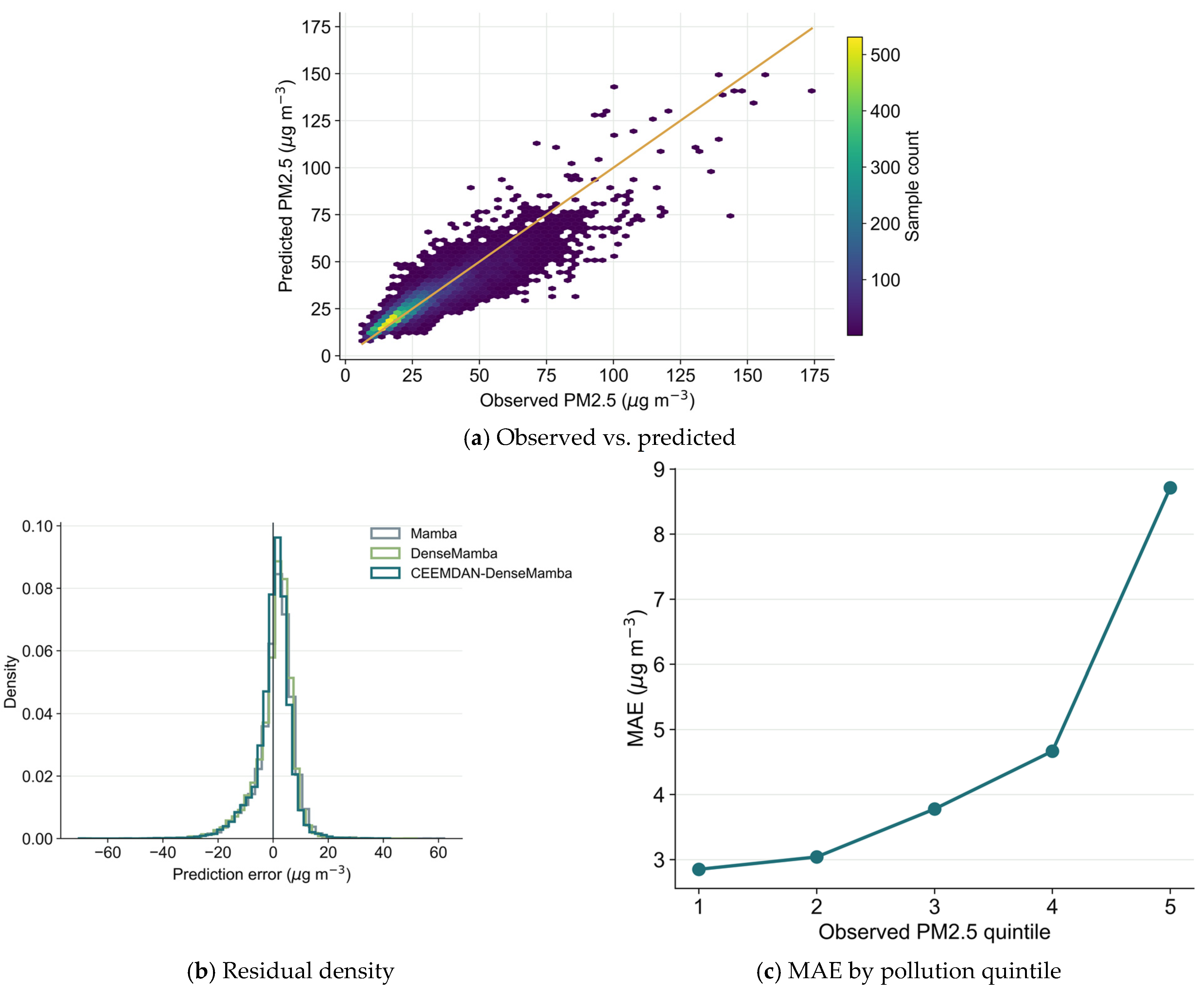
Beyond the aggregate metrics, Figure 9 examines test-set prediction diagnostics from three complementary perspectives. Panel a compares ChinaHighPM2.5 reference values with CEEMDAN-DenseMamba predictions; panel b compares residual-density curves for representative models; and panel c reports mean absolute error across reference-concentration quintiles. The wider spread at high concentrations indicates more difficult cases. 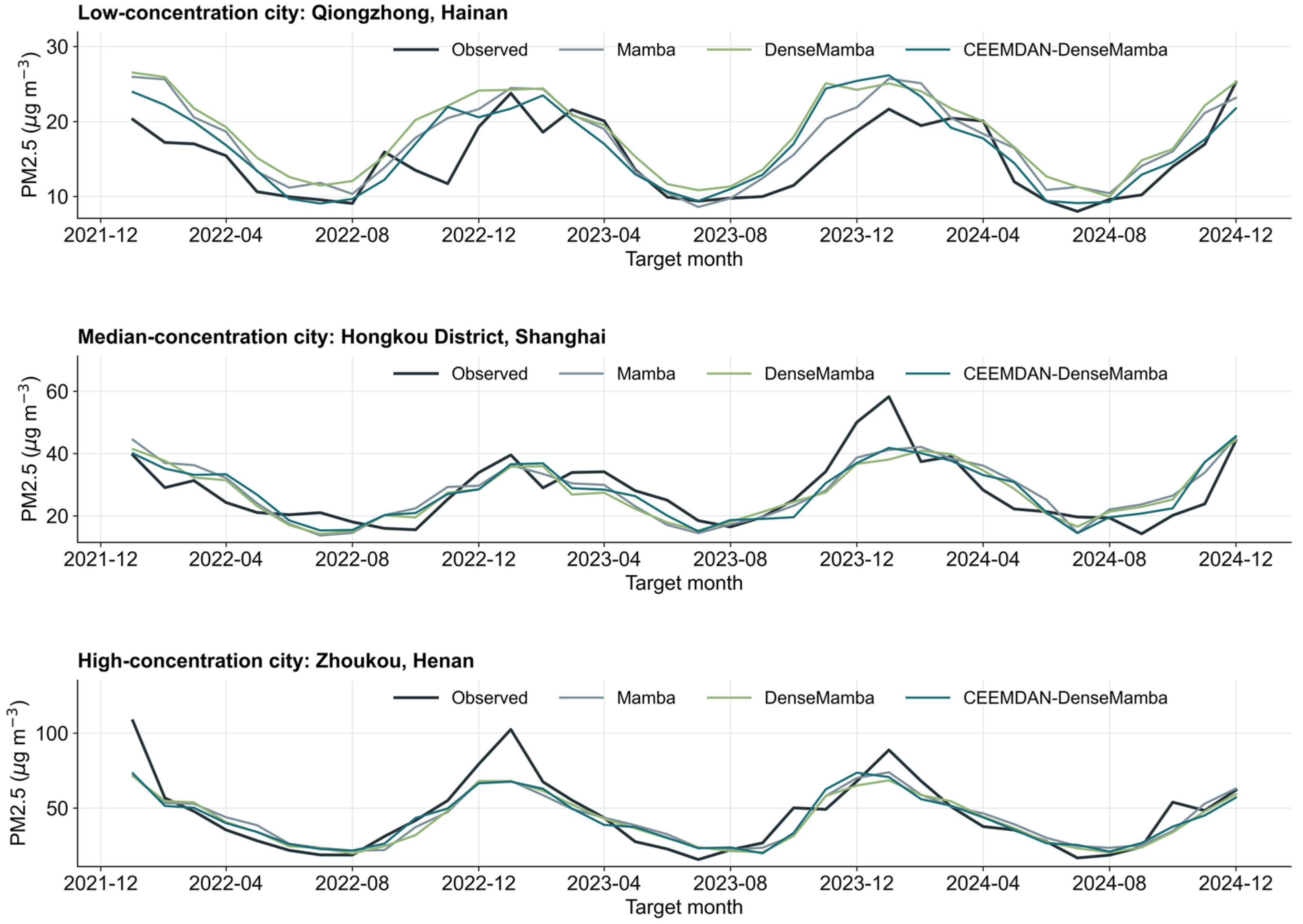In Figure 9, Figure 10 and Figure 11, “observed” denotes the reconstructed ChinaHighPM2.5 reference target rather than a direct monitoring-only observation.

Representative city-level trajectories are compared in Figure 10 for cities with low, median, and high PM2.5 reference concentrations. The stacked trajectories plot the ChinaHighPM2.5 reference series and model predictions for the selected cities, showing whether the model tracks seasonal peaks, low-concentration troughs, and stage-wise changes. This city-level visualization complements pooled metrics by displaying the temporal form of prediction errors for known cities.

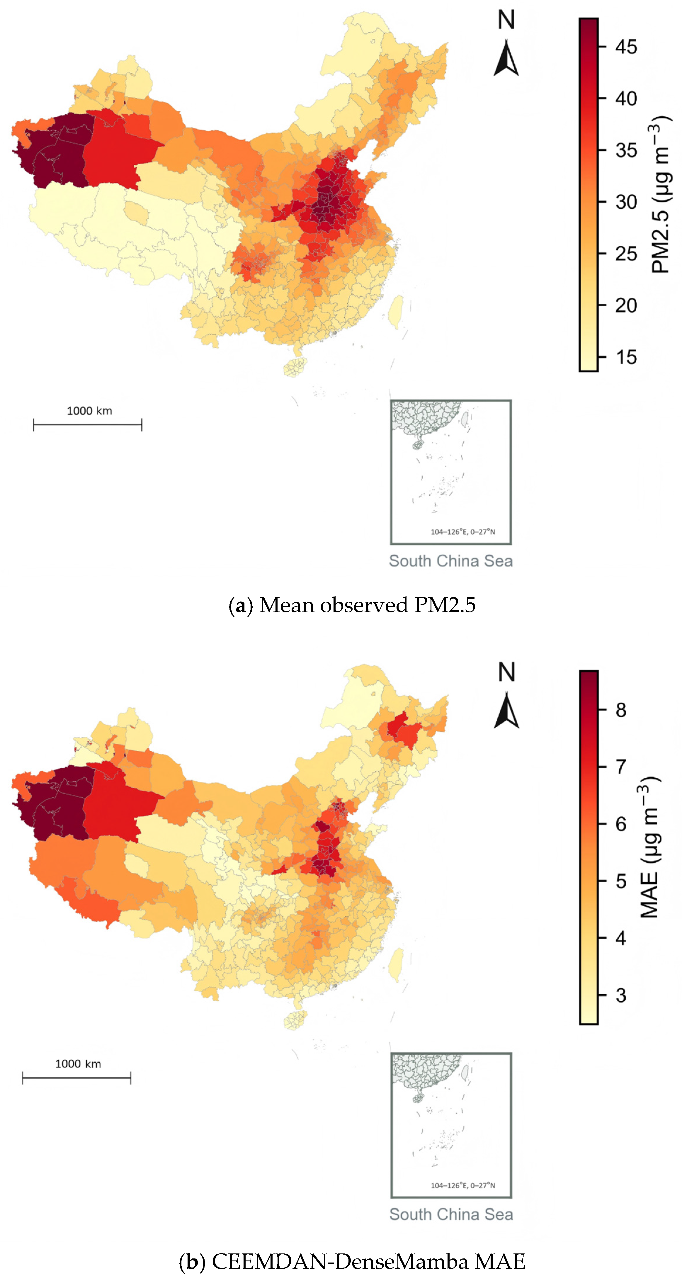
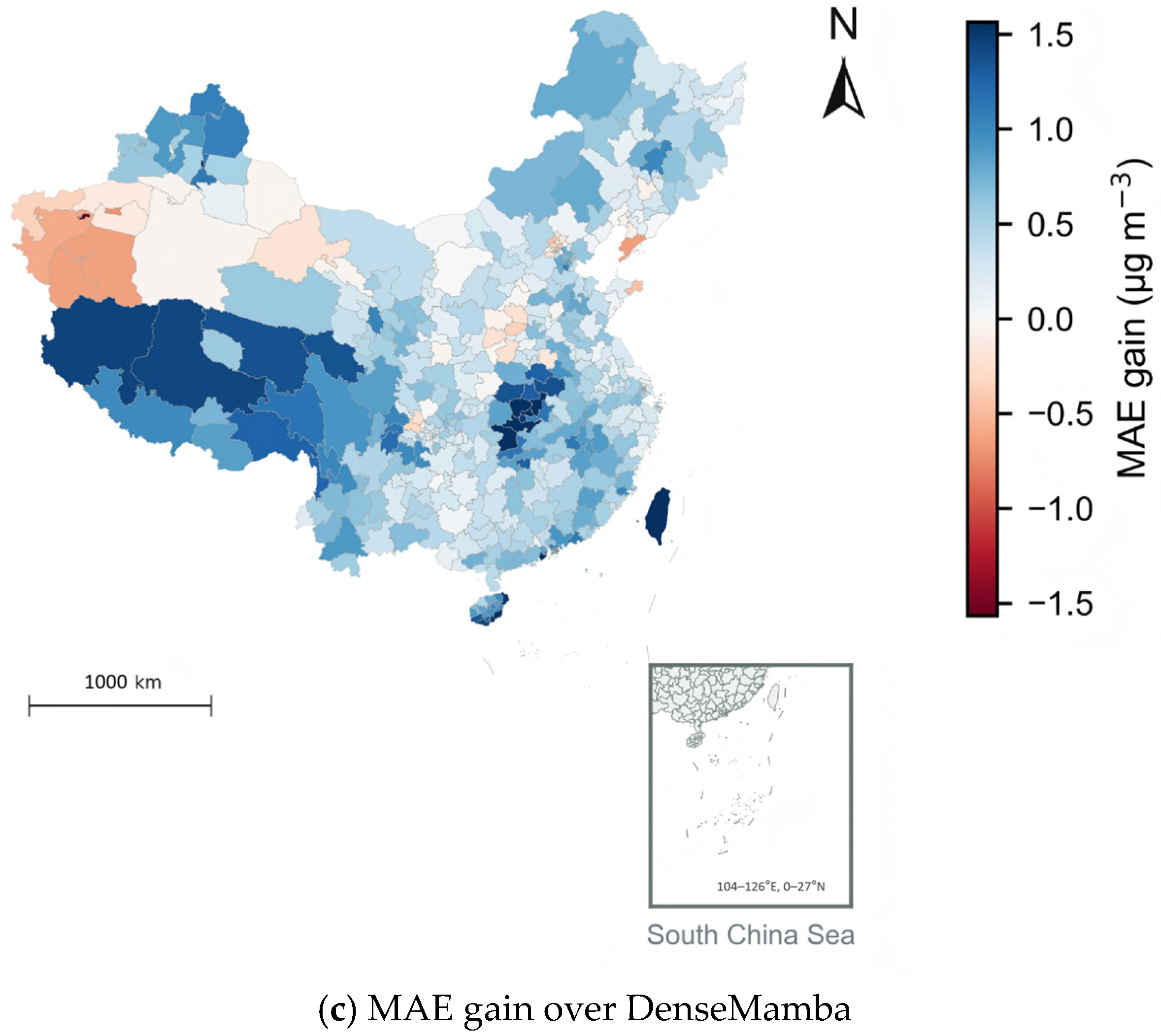
The spatial maps in Figure 11 link model performance back to geography. Panel a maps the mean ChinaHighPM2.5 reference concentration during the test period; panel b shows city-level MAE for CEEMDAN-DenseMamba; and panel c maps the MAE gain relative to DenseMamba, with positive values indicating lower MAE for CEEMDAN-DenseMamba. These maps characterize spatial heterogeneity of error among the 475 cities already represented during training; they do not constitute a test of transfer to unseen cities or regions.

3.3. Backbone and Decomposition Comparisons, Robustness, and Auxiliary Diagnostics

To further isolate the role of the decomposition strategy, three alternative-decomposition models—EMD-DenseMamba, EEMD-DenseMamba, and FFT-DenseMamba—are introduced under the DenseMamba backbone and compared with CEEMDAN-DenseMamba. Table 5 and

Table 6. Test-set performance of decomposition-enhanced DenseMamba models.

Model Variant	Input Type	RMSE	MAE	${\mathit{R}}^{\mathbf{2}}$	MAPE (%)	Corr
CEEMDAN- DenseMamba	CEEMDAN- enhanced	6.931 ± 0.047	4.833 ± 0.066	0.801 ± 0.003	18.084 ± 0.524	0.896 ± 0.002
EMD- DenseMamba	EMD- enhanced	7.060 ± 0.131	4.936 ± 0.123	0.794 ± 0.008	18.681 ± 0.822	0.893 ± 0.004
EEMD- DenseMamba	EEMD- enhanced	7.316 ± 0.210	5.186 ± 0.433	0.778 ± 0.013	20.092 ± 3.472	0.887 ± 0.003
FFT- DenseMamba	FFT- enhanced	7.018 ± 0.175	4.969 ± 0.285	0.796 ± 0.010	18.692 ± 2.401	0.894 ± 0.005

summarize the primary benchmark rather than a single optimization-controlled ablation.

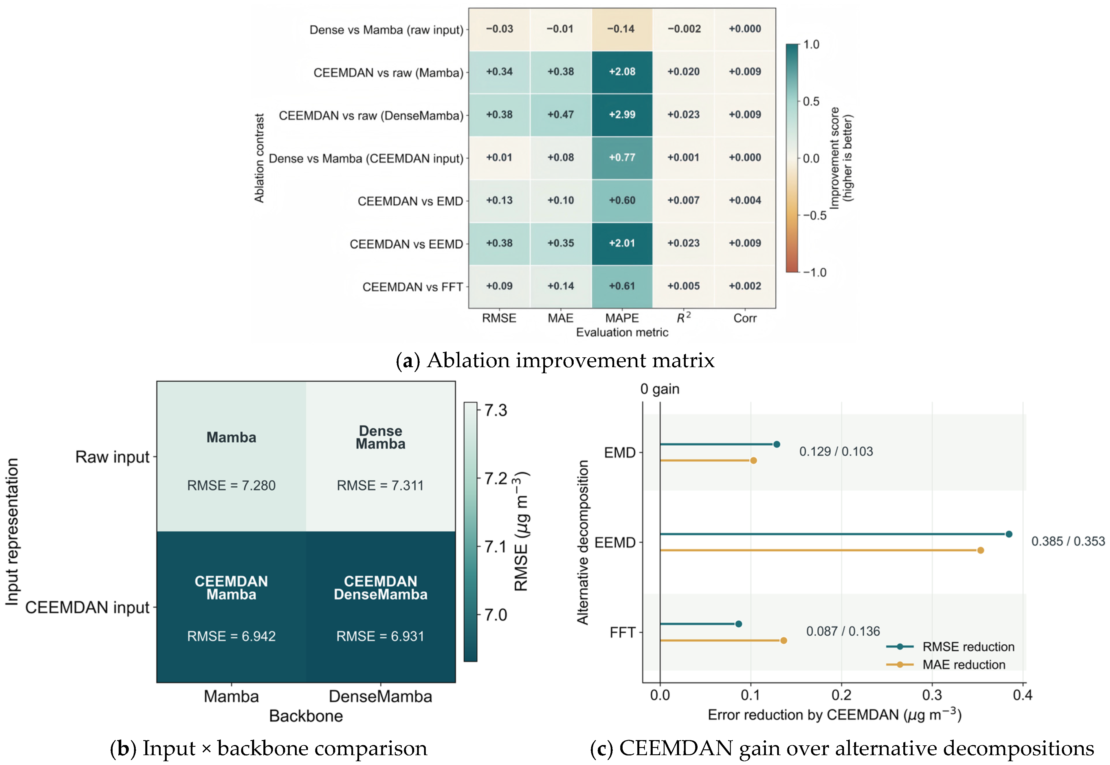
Figure 12 presents descriptive contrasts within the primary benchmark. Panel a reports metric-wise differences among selected pairs; panel b organizes the non-decomposition and CEEMDAN-enhanced benchmark results under Mamba and DenseMamba; and panel c compares CEEMDAN with EMD, EEMD, and FFT under the DenseMamba backbone, where those four decomposition-enhanced DenseMamba models share identical architecture and training settings. The structural contrasts involving Mamba versus DenseMamba are not treated as optimization-controlled effects in this figure and are interpreted together with the equal-optimization reruns.

The quantitative differences in Table 6 show that CEEMDAN-DenseMamba has mean RMSE values 1.83%, 5.26%, and 1.24% lower than EMD-DenseMamba, EEMD-DenseMamba, and FFT-DenseMamba, respectively, with corresponding MAE reductions of 2.09%, 6.81%, and 2.74%. Because the differences relative to EMD and FFT are small, they are interpreted as benchmark-level mean differences rather than universal or statistically established superiority of CEEMDAN.

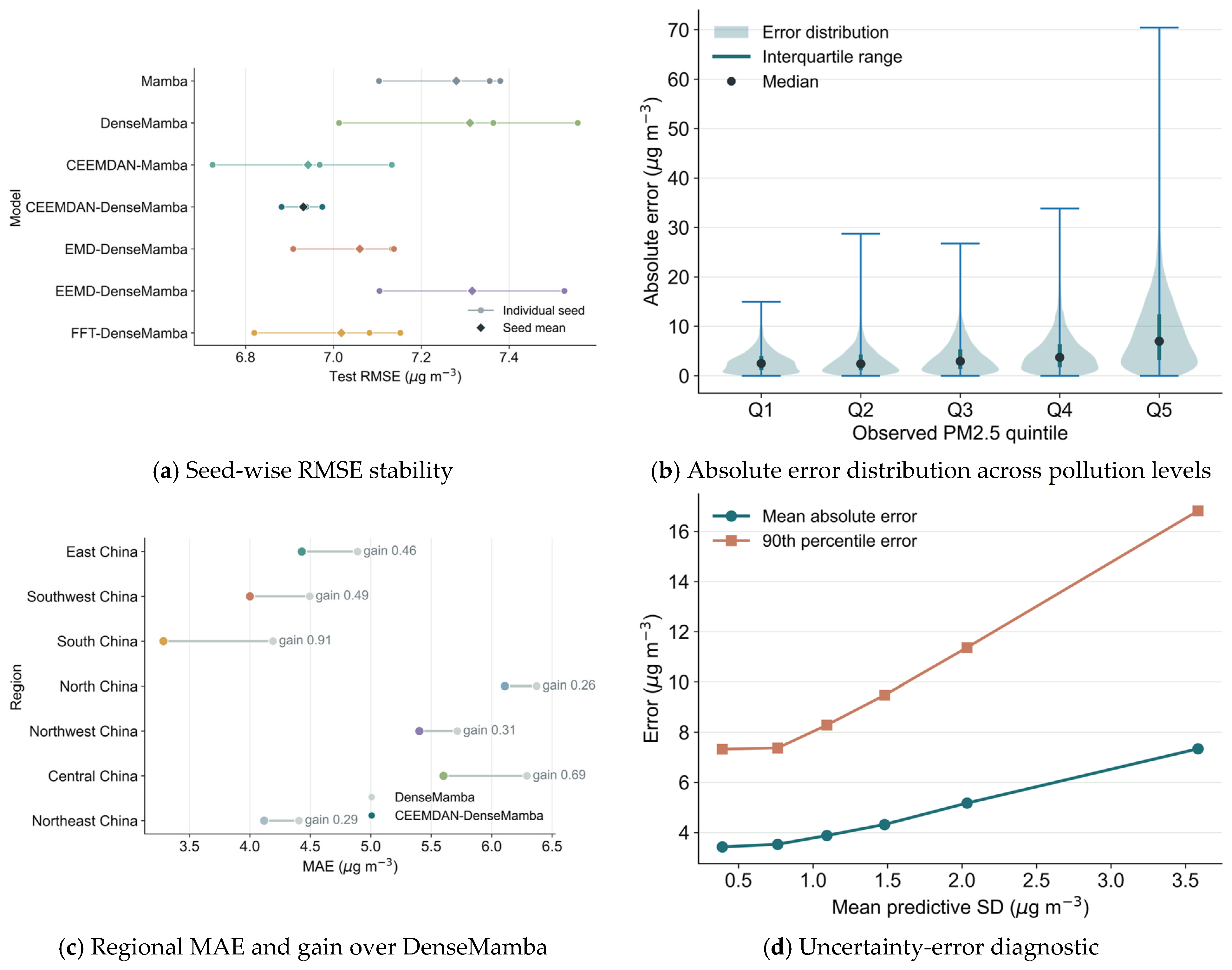
Robustness and error heterogeneity are further examined in Figure 13 from several complementary perspectives. Panel a compares seed-wise root mean squared error across the seven models, showing whether the main ranking is sensitive to random initialization. Panel b presents absolute-error distributions across reference-concentration quintiles, indicating how error magnitude changes from low- to high-concentration samples. Panel c summarizes regional mean absolute error together with the gain over DenseMamba, revealing regional differences in both baseline difficulty and decomposition-related improvement. Panel d relates cross-seed predictive variability to mean and upper-tail errors, providing an additional check on whether larger predictive variability corresponds to larger realized errors. These diagnostics show how run-to-run variability and prediction error differ across seeds, pollution levels, and regions; paired uncertainty for the structural contrasts is evaluated in the controlled analysis that follows.

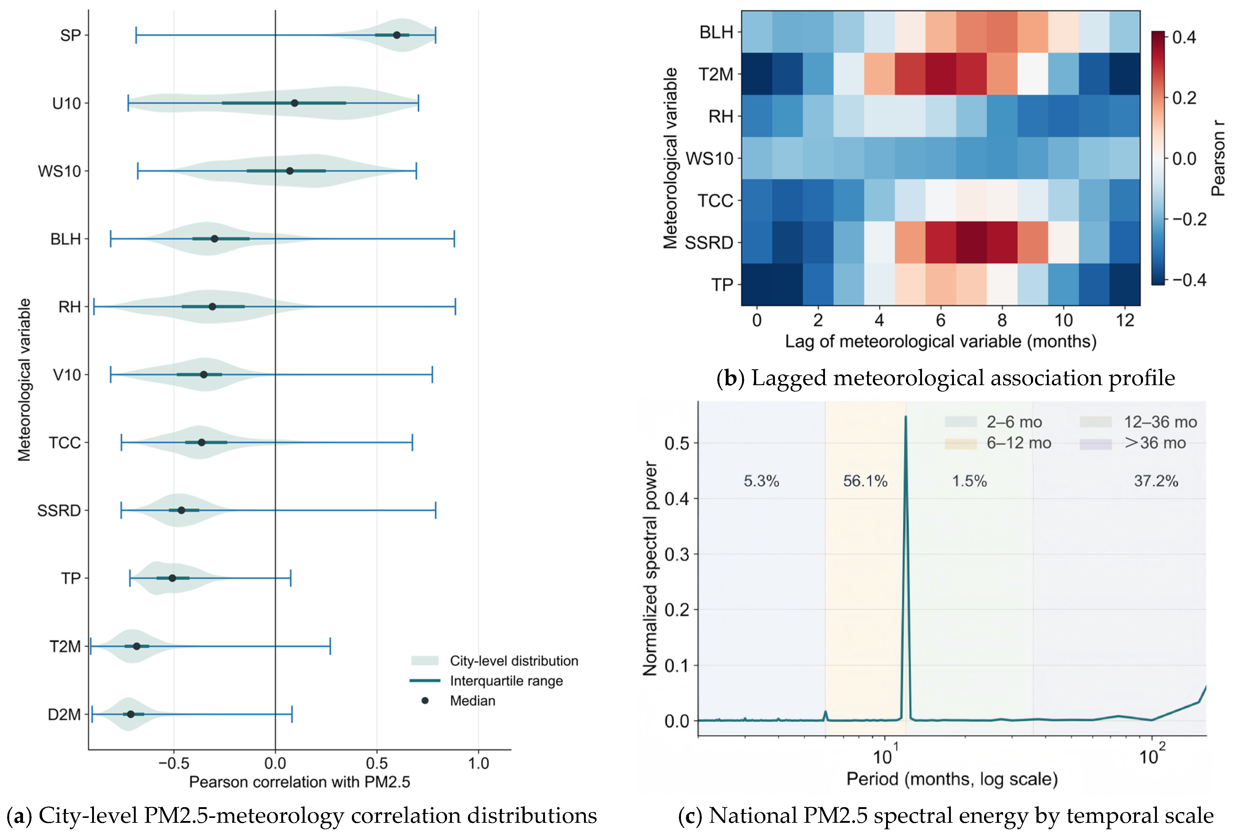
As an auxiliary diagnostic, Figure 14 examines feature-level associations and temporal-scale structure rather than formal causal attribution. Panel a summarizes city-level correlation distributions between PM2.5 and meteorological variables, showing heterogeneity in how local PM2.5 changes are associated with pressure, wind, boundary-layer height, humidity, radiation, precipitation, and temperature. Panel b presents the lagged meteorological association profile, indicating that several meteorological variables have synchronous and delayed relationships with PM2.5. Panel c shows the national PM2.5 spectral energy by temporal scale, highlighting the coexistence of intra-annual, annual, multi-year, and low-frequency components. These diagnostics support the use of meteorological drivers and multi-scale decomposition, while avoiding an overinterpretation of individual feature effects as direct causal contributions.

Table 5 and Table 6 summarize the primary benchmark rather than a single optimization-controlled ablation. CEEMDAN-DenseMamba has the lowest mean RMSE and MAE among the seven primary-benchmark models, while the four decomposition-enhanced DenseMamba variants provide a direct decomposition-method comparison under matched backbone and training settings. Because the remaining structural pairs use different pre-specified optimization configurations, the benchmark alone does not establish whether their differences arise from architecture, decomposition, or optimization. The controlled analysis that follows therefore adds equal-optimization reruns, paired confidence intervals, a parameter-matched GRU, local sensitivity to $K$, and city-wise diagnostics.

3.4. Controlled Attribution, Sensitivity, and City-Wise Diagnostics

To separate structural effects from optimizer differences, Mamba, DenseMamba, CEEMDAN-Mamba, and CEEMDAN-DenseMamba were retrained using one identical configuration pre-specified before test-set evaluation: learning rate 1.5 × 10⁻⁴, AdamW weight decay 5 × 10⁻⁶, scheduler patience 10, early-stopping patience 35, minimum 30 epochs, maximum 120 epochs, batch size 128, gradient clipping 5.0, and dropout 0.2. The same seeds (42, 52, and 62), chronological split, preprocessed tensors, model definitions, and the same cached history-only CEEMDAN components used in the primary benchmark were retained. A two-layer GRU with a hidden size of 192 was added as a parameter-matched non-decomposition baseline; its 368,641 trainable parameters closely match the 369,281 parameters of Mamba. The corresponding equal-optimization results and parameter-matched baseline are reported in

Table 7. Equal-optimization structural rerun and parameter-matched baseline.

Model	Input Type	Trainable Parameters	RMSE	MAE	${\mathit{R}}^{\mathbf{2}}$	MAPE (%)	Corr
Mamba	27-dim non-decomposition	369,281	7.242 ± 0.133	5.158 ± 0.144	0.783 ± 0.008	19.591 ± 0.579	0.887 ± 0.005
DenseMamba	27-dim non-decomposition	534,657	6.980 ± 0.090	4.921 ± 0.050	0.798 ± 0.005	18.622 ± 0.257	0.895 ± 0.002
CEEMDAN-Mamba	$31\text{-}\dim , K=4$	369,793	7.212 ± 0.347	5.219 ± 0.309	0.784 ± 0.020	20.359 ± 1.395	0.888 ± 0.011
CEEMDAN-DenseMamba	$31\text{-}\dim , K=4$	535,169	6.860 ± 0.112	4.823 ± 0.036	0.805 ± 0.006	18.133 ± 0.158	0.899 ± 0.004
GRU-matched	27-dim non-decomposition	368,641	6.862 ± 0.183	4.771 ± 0.033	0.805 ± 0.010	17.582 ± 1.136	0.902 ± 0.005

.

Under identical optimization, DenseMamba reduced mean RMSE and MAE relative to Mamba, and CEEMDAN-DenseMamba reduced both errors relative to CEEMDAN-Mamba. In contrast, the incremental CEEMDAN effect within a fixed backbone was smaller. The parameter-matched GRU was highly competitive, with an RMSE nearly identical to CEEMDAN-DenseMamba and a lower mean MAE. This result indicates that the $L=12$ setting does not by itself demonstrate a unique long-sequence advantage for the Mamba-inspired backbone.

Paired uncertainty was assessed by a moving-block bootstrap over the 36 target months. For each model, predictions were first averaged across the three initialization seeds. Consecutive six-month blocks were then resampled 2000 times from these seed-averaged prediction matrices, and each selected month retained all 475 cities so that the cross-city structure within a month was preserved. Negative differences in

Table 8. Paired moving-block bootstrap intervals for equal-optimization structural contrasts.

Comparison	$\Delta \mathbf{RMSE}$	95% Confidence Interval for $\mathbf{\Delta }\mathbf{RMSE}$	$\mathbf{\Delta }\mathbf{MAE}$	95% Confidence Interval for $\mathbf{\Delta }\mathbf{MAE}$
CEEMDAN-Mamba vs. Mamba	−0.115	[−0.331, 0.075]	−0.003	[−0.171, 0.125]
CEEMDAN-DenseMamba vs. DenseMamba	−0.105	[−0.245, 0.129]	−0.100	[−0.202, 0.056]
DenseMamba vs. Mamba	−0.314	[−0.594, −0.178]	−0.267	[−0.456, −0.180]
CEEMDAN-DenseMamba vs. CEEMDAN-Mamba	−0.305	[−0.498, −0.080]	−0.364	[−0.530, −0.180]

favor the first model.

The intervals for DenseMamba vs. Mamba and CEEMDAN-DenseMamba vs. CEEMDAN-Mamba exclude zero for both RMSE and MAE, providing evidence for a dense-connection benefit under the common optimization setting. By contrast, the CEEMDAN-Mamba vs. Mamba and CEEMDAN-DenseMamba vs. DenseMamba intervals cross zero, so the incremental CEEMDAN effect is not uniformly resolved under the stricter paired analysis. These results motivate a more cautious decomposition claim than the ranking of the primary benchmark alone would suggest.

A local sensitivity check varied the retained CEEMDAN component count without changing the common optimization protocol. For $K=2$, $K=3$, and $K=4$, CEEMDAN-DenseMamba obtained RMSE values of 6.902 ± 0.074, 6.986 ± 0.329, and 6.860 ± 0.112; MAE values of 4.736 ± 0.030, 5.013 ± 0.445, and 4.823 ± 0.036; and $R^2$ values of 0.803 ± 0.004, 0.798 ± 0.019, and 0.805 ± 0.006, respectively. $K=4$ has the lowest mean RMSE and highest mean $R^2$, whereas $K=2$ has the lowest mean MAE. The behavior therefore does not collapse when $K$ is locally reduced, but the experiment does not establish $K=4$ as a globally optimal component count.

To distinguish pooled performance from within-city temporal tracking, the equal-optimization runs were also evaluated with city-wise metrics.

Table 9. Pooled and city-wise diagnostics under the equal-optimization protocol.

Model	Pooled RMSE	Mean City RMSE	Median City RMSE	City RMSE IQR	Median City ${\mathit{R}}^{\mathbf{2}}$	Positive City ${\mathit{R}}^{\mathbf{2}}$	Anomaly RMSE
Mamba	7.242 ± 0.133	6.779 ± 0.116	6.207 ± 0.122	5.216–7.874	0.660 ± 0.012	95.1%	6.921 ± 0.158
DenseMamba	6.980 ± 0.090	6.554 ± 0.077	6.055 ± 0.052	5.041–7.642	0.663 ± 0.010	95.8%	6.759 ± 0.034
CEEMDAN-Mamba	7.212 ± 0.347	6.779 ± 0.362	6.122 ± 0.365	5.206–7.661	0.639 ± 0.032	93.3%	6.890 ± 0.267
CEEMDAN-DenseMamba	6.860 ± 0.112	6.430 ± 0.113	5.903 ± 0.183	4.804–7.461	0.670 ± 0.013	95.3%	6.683 ± 0.079
GRU-matched	6.862 ± 0.183	6.398 ± 0.155	5.894 ± 0.324	4.712–7.577	0.699 ± 0.016	96.0%	6.527 ± 0.149

reports the mean city RMSE, median city RMSE and interquartile range (IQR), median city $R^2$, the fraction of cities with positive $R^2$, and anomaly RMSE after removing each city’s test-period mean.

The city-wise diagnostics show that the models track temporal variation within most known cities rather than relying only on pooled between-city differences; however, the parameter-matched GRU remains competitive or better on several city-wise measures. These results therefore support temporal forecasting for the known 475 cities but not spatial transfer to unseen cities.

Finally, a successive-origin overlap diagnostic was applied to the cached CEEMDAN components to examine right-edge sensitivity. Across all true-CEEMDAN windows, overlap correlations were 0.883, 0.903, 0.642, and 0.630 for IMF1–IMF4, respectively. The lower stability of higher-order components confirms that rolling-window modes are not invariant to extension of the right edge. Accordingly, individual IMF channels are used as predictive features rather than assigned fixed physical meanings, and broader sensitivity to window length or boundary-extension rules remains a limitation.

4. Discussion

The primary seven-model benchmark identifies CEEMDAN-DenseMamba as the lowest-error model within that original comparison, but the additional controlled analyses refine the interpretation of why. Under identical optimization, the dense-connection contrasts show paired reductions in RMSE and MAE with confidence intervals below zero, whereas the incremental CEEMDAN effect within a fixed backbone is smaller and its paired confidence intervals cross zero. The decomposition front end therefore provides an inspectable multi-scale representation and a temporally valid alternative to full-series decomposition, but the current evidence does not support a universal claim that CEEMDAN itself always improves a fixed backbone. This distinction strengthens the transparency of performance attribution and separates predictive evidence from physical causal interpretation.

Within the matched DenseMamba decomposition comparison, CEEMDAN has lower mean errors than EMD, EEMD, and FFT, although the margins relative to EMD and FFT are modest. A plausible methodological explanation is that CEEMDAN combines adaptive local decomposition with ensemble noise assistance [22,23]. Whereas FFT uses fixed frequency masks, EMD and EEMD exhibit distinct sensitivities to mode mixing and noise. These mechanisms are discussed as possible reasons for the observed benchmark differences rather than as proof that CEEMDAN is universally superior. The successive-origin diagnostic further shows that higher-order rolling modes are sensitive to the window edge, so individual components should not be assigned fixed physical meanings.

The parameter-matched GRU provides an important boundary in relation to the Mamba interpretation. With 368,641 trainable parameters versus 369,281 for Mamba, the GRU achieves an equal-optimization RMSE of 6.862 ± 0.183 and MAE of 4.771 ± 0.033, remaining competitive with CEEMDAN-DenseMamba and outperforming non-decomposition Mamba under the present $L=12$ setting. A 12-month context already spans one annual cycle and is too short to demonstrate the long-sequence computational advantage usually associated with Mamba. Accordingly, this study uses Mamba-inspired blocks as a sequence-modeling backbone for controlled feature and architecture comparisons rather than claiming that they are intrinsically superior to recurrent forecasting models.

Several limitations remain. First, temporal validation uses one fixed future test period (January 2022–December 2024). The three random seeds and paired bootstrap quantify initialization and prediction-error uncertainty but do not replace rolling-origin evaluation across multiple historical regimes. Second, all test samples come from the same 475 city-level units represented in training; the results therefore demonstrate temporal generalization to future months for known cities, not spatial transfer to unseen cities or regions. Third, the sensitivity analysis for $K$ is limited to $K\in \left\{2,3,4\right\}$, and rolling-window length, CEEMDAN trial count, boundary extension, and residual inclusion have not been exhaustively varied. The successive-origin analysis also shows lower stability for higher-order rolling IMFs. Fourth, ChinaHighPM2.5 is a reconstructed target product rather than a direct monitoring-only series, so dependence between target reconstruction and meteorological information may affect some predictor associations. Finally, the study does not provide a broad comparison against all recent Transformer, graph, or Mamba-family forecasting methods [15,16,17,19,28,29,30,31,32]. The reported results should therefore be interpreted within the present monthly, known-city, fixed-split setting.

Future work should retain the same history-only feature-construction rule while extending evaluation to rolling-origin test windows, multi-step forecasting, unseen-city or cross-region transfer, broader rolling-window and decomposition-parameter sensitivity, and stronger external baselines. These extensions should follow established principles for forecasting evaluation, time-series validation, and predictive accuracy comparison [45,46,47]. Multi-scale decomposition could also be combined with graph neural networks, dynamic spatial adjacency, or pollutant-transport priors [16,18,19]. Stronger claims about decomposition or backbone generality require consistent evidence across additional temporal scales, regions, and model families.

5. Conclusions

This study develops a temporally constrained rolling-decomposition and Mamba-family forecasting framework for monthly PM2.5 prediction across 475 city-level regions in China. The primary benchmark contains Mamba, DenseMamba, CEEMDAN-Mamba, CEEMDAN-DenseMamba, EMD-DenseMamba, EEMD-DenseMamba, and FFT-DenseMamba, all evaluated on the same chronological split and repeated-seed protocol. Additional controlled analyses retain the original data and decomposition cache while adding equal-optimization structural checks, paired uncertainty intervals, a parameter-matched GRU, local sensitivity to $K$, and city-wise diagnostics.

In the primary seven-model benchmark, CEEMDAN-DenseMamba has the lowest mean RMSE and MAE. Under identical optimization, the dense-connection contrasts show paired RMSE and MAE intervals below zero, whereas the incremental CEEMDAN contrasts within fixed backbones are smaller and their intervals cross zero. The parameter-matched GRU remains highly competitive, and local sensitivity across $K\in \left\{2,3,4\right\}$ does not identify a single universally optimal component count. Together, these findings support the value of temporally valid, inspectable multi-scale feature construction and transparent performance attribution rather than a universal superiority claim for CEEMDAN or Mamba. The conclusions are limited to monthly future-month forecasting for the 475 known cities, the 2000–2024 data product, the specified feature construction, and the fixed temporal test period.