A Concept-Bottleneck Explainable AI Framework for Diagnosing Agile Delivery Outcomes

Abstract

Agile outcome models commonly map Jira variables directly to a retrospective label and then explain the prediction through fragmented feature attributions; they rarely separate domain concepts, team clustering, unresolved work, and concept-label coupling. This study evaluates a domain-informed, concept-bottleneck-style explainable AI architecture for retrospective diagnosis of Agile Epic outcomes. A frozen Jira export of 10,000 unique issue-level records was linked to a pre-specified analytical cohort of 180 Epics across 14 teams. Six experts rated efficiency, effectiveness, sustainability, and contextual risk, while outcomes were recorded as Successful, Challenged, or Unsuccessful. Because the outcome labels and concept ratings were informed by the same Jira evidence, the models estimate consistency with an expert labelling procedure, rather than independent project success. Under five-fold group-aware cross-validation, the fixed-configuration flat LightGBM achieved macro-F1 = 0.864 ± 0.053 and the fixed-configuration HMXAI/CBM-style model achieved 0.843 ± 0.084. These descriptive primary scores are not a joint nested-model-selection comparison. The proposed method, therefore does, not demonstrate a performance improvement; its contribution is an inspectable diagnostic structure. Performance fell materially on the resolved-only subset (LightGBM macro-F1 = 0.645), and model-specific nested, leave-one-team-out, calibration, uncertainty, correlation, and intervention analyses further bound the claims. Concept interventions were not uniformly monotone, so the concept layer is domain-interpretable in form but not yet user-validated as actionable. The study contributes a transparent audit of when concept-level diagnosis can complement flat classification and when circularity, censoring, and shortcut learning restrict interpretation.

1. Introduction

Agile project management has become a dominant approach for delivering software-intensive and technology-driven work, particularly in contexts characterised by uncertainty, evolving requirements, iterative delivery, and rapid technological change [1,2,3]. However, assessing whether an Agile delivery initiative is successful remains difficult. Agile outcomes are shaped not only by schedule, cost, and scope, but also by dependency management, defect exposure, completion behaviour, team continuity, organisational support, customer value, and the ability to sustain delivery over time [4,5,6].

Traditional project success assessment has often been associated with the iron triangle of time, cost, and scope. These criteria remain relevant, but they provide only a partial view of success in Agile environments [7,8]. An initiative may satisfy planned constraints while accumulating technical debt or failing to deliver meaningful value. Conversely, an initiative may deviate from early expectations yet still be considered valuable if it produces usable outcomes, supports organisational learning, and strengthens future delivery capability. Agile project success is therefore better treated as a multidimensional construct, rather than a single operational metric [9,10,11,12].

Machine-learning methods have increasingly been applied to software and project-management prediction tasks, including effort estimation, story-point prediction, defect prediction, risk assessment, and project status classification [13,14,15]. Many of these studies use flat models in which all input features are directly mapped to an outcome. Such models can be accurate, but they do not necessarily explain whether a predicted outcome is driven by efficiency, effectiveness, sustainability, or contextual risk. This limits their value for Agile managers, who typically need diagnostic explanations rather than only risk scores.

Explainable AI can help by identifying influential features through, for example, SHapley Additive exPlanations (SHAP) [16,17,18]. Yet feature-level explanations alone may still be too fragmented for managerial action. A project manager may need to know whether an Epic is at risk because of poor completion flow, inadequate value realisation, unstable delivery capacity, or high contextual risk [19,20,21]. Therefore, there is value in linking feature-level evidence to higher-level concepts that practitioners recognise.

This study evaluates a domain-informed hierarchy related to concept bottleneck models (CBMs) [22,23,24,25,26]. Raw Jira evidence is mapped to four expert-labelled concepts, and only those predicted concepts are passed to the outcome stage. The architecture is not a new general-purpose algorithm and is not expected to improve accuracy automatically. It is evaluated as a constrained diagnostic representation whose value depends on concept fidelity, intervention behaviour, uncertainty, and the degree of concept-label coupling.

The study is guided by three research questions. RQ1 asks how accurately Jira-derived Epic evidence reproduces retrospectively expert-validated outcome labels under team-grouped and nested sensitivity analyses. RQ2 asks whether the concept bottleneck provides a stable diagnostic representation, assessed through fidelity, correlation, leakage, calibration, uncertainty, separability, and intervention monotonicity, rather than through assumed managerial usefulness. RQ3 asks which Jira indicators and concepts dominate the reproduced labels and how strongly those findings depend on unresolved process states.

The contribution is threefold. First, the study operationalises an expert-informed Jira diagnostic rubric at Epic level. Second, it compares flat and concept-bottleneck-style structures while making explicit that the proposed hierarchy does not outperform the best flat candidate. Third, it audits failure modes often hidden in applied Agile analytics: shared-evidence labelling, process-state shortcuts, right-censoring, team clustering, concept correlation and leakage, calibration, uncertainty, non-monotone interventions, and the absence of practitioner validation.

The remainder of the paper is organised as follows. Section 2 reviews Agile success, machine learning in Agile project prediction, explainable AI, concept bottleneck models, and related studies. Section 3 describes the dataset, expert-rating procedure, leakage and circularity controls, modelling strategy, and evaluation design. Section 4 presents the empirical results. Section 5 discusses theoretical and managerial implications. Section 6 concludes the paper and outlines limitations and future research.

2. Literature Review

This review is organised around the multidimensional definition of Agile outcomes, supervised and unsupervised learning, explainable AI, and concept-bottleneck modelling. The distinction matters because supervised methods optimise against an explicit label and are therefore exposed to label construction and leakage, whereas unsupervised and transfer-learning methods discover or align representations without task labels, but do not by themselves solve outcome validity.

2.1. Agile Project Success as a Multidimensional Construct

Project success has traditionally been assessed using criteria such as time, cost, and scope [7,8]. These indicators remain useful because they describe whether delivery occurred within expected constraints. However, Agile work is iterative, adaptive, and value-driven; therefore, compliance with an initial plan is not sufficient to determine success [27,28]. Agile success depends on whether an initiative delivers usable value, maintains stakeholder alignment, preserves team capability, and manages technical and organisational complexity [29,30]. Recent case-based work likewise shows that Story Points alone can obscure delivery flow and operational reliability, and should be complemented by flow and service-performance indicators [31].

In this study, Agile delivery success is organised around four concepts. Efficiency refers to delivery flow, completion behaviour, resource use, and workload control. Effectiveness refers to value realisation, product quality, and useful completion of work. Sustainability refers to whether the delivery pattern is maintainable from a team and organisational perspective. Contextual risk refers to dependencies, technical debt, priority pressure, uncertainty, and other conditions that make delivery difficult. These dimensions are not independent in practice; they jointly shape whether an Epic is successful, challenged, or unsuccessful.

Theoretical Derivation of the Four Diagnostic Concepts

The four concepts were selected from the project-success and project-complexity literature, rather than derived only from the Jira dataset. Efficiency reflects the traditional concern with delivery performance and resource use, but is broadened here to include flow and completion behaviour visible in Agile delivery traces. Effectiveness reflects the long-standing distinction between project management success and product or business success, emphasising whether delivered work appears usable and value-bearing, rather than merely completed. Sustainability captures the capacity to maintain delivery over time, including continuity, workload dispersion, and team-level delivery health. Contextual risk captures the complexity, dependency, uncertainty, and technical or organisational constraints surrounding the Epic. This structure is consistent with multidimensional views of project success and project complexity [7,8,29,30,32], while remaining operational enough to be represented as a concept layer in a CBM-style architecture.

2.2. Supervised and Unsupervised Learning for Software and Delivery Analytics

2.2.1. Supervised Learning

Supervised learning has been used for story-point and effort estimation, defect prediction, status classification, and other software-engineering targets [13,14,15,33]. These models learn a mapping from observed variables to a supplied target; consequently, validation quality depends on whether the target is independent of the predictors. Yan et al. [34], for example, combine machine vision with physics-informed neural constraints for supervised pantograph–catenary state detection. Although the application domain is different, the study illustrates how domain structure can regularise a supervised model. In the present study, the corresponding domain structure is an expert-labelled concept layer, but the target remains retrospective and evidence-coupled.

2.2.2. Unsupervised and Transfer Learning

Unsupervised learning and unsupervised domain adaptation seek structure or cross-domain alignment without labelled target examples. Wang et al. [35] use spatial-channel multi-scale graph interaction and deep transfer learning for unsupervised rotating-machinery fault diagnosis. Such methods are relevant methodologically because they reduce dependence on target labels, but they are not direct benchmarks for Agile outcome diagnosis: the sensor inputs, fault targets, temporal assumptions, and absence of expert concept ratings differ fundamentally. An unsupervised Agile extension could discover delivery archetypes, but it would not validate whether those archetypes represent business success.

Across supervised and unsupervised studies, external validity requires evaluation that respects the unit of deployment. Project data contain clustered observations from teams, products, workflows, and organisations. Ignoring these levels can inflate performance. The present dataset supports grouping by Team_ID, but it does not contain a separate Project_ID or Product_ID; higher-level cross-team clustering, therefore, cannot be tested, and is reported as an unresolved validity limitation. Cross-site validation designs in other fields [36] are methodologically informative, but their numerical results are not comparable with the present target.

2.3. Explainable AI and Managerial Interpretability

Explainable AI methods aim to make model behaviour more understandable to users. SHAP is widely used because it estimates how much each feature contributes to a prediction and can be summarised locally or globally [16,17,18]. In Agile project analytics, SHAP can identify influential evidence such as completion ratio, abandoned work, bug ratio, or dependency count.

However, feature-level explanation does not automatically produce managerial interpretability. A practitioner may not only ask which feature mattered, but what type of delivery problem is indicated. A completion problem, a defect problem, a sustainability problem, and a dependency problem require different interventions [19,20,21,37,38,39]. Therefore, Agile XAI needs to connect feature-level evidence to project-management concepts [22,26].

2.4. Concept Bottleneck Models and Domain-Informed Hierarchies

The proposed architecture is a concept-bottleneck-style model, rather than a new machine-learning algorithm. CBMs predict human-interpretable concepts before the target [22,26]. Their appeal includes the possibility of expert intervention, yet leakage between concept probabilities and labels can preserve predictive information that is not semantically represented [25], and intervention efficacy cannot be assumed [40]. Hybrid and stochastic CBM variants [23,24] address related accuracy–flexibility trade-offs, but they are not direct benchmarks here because they were developed for different modalities and concept annotations.

The architecture also resembles stacked generalisation because lower-stage outputs enter a higher-stage model. The safeguard is that the second stage is trained only on inner out-of-fold concept predictions, never on concept values fitted to the full dataset. The intermediate variables are expert-labelled Agile dimensions, rather than arbitrary ensemble scores. Their usefulness must therefore be tested through fidelity, uncertainty, correlation, concept-label coupling, and controlled interventions, not inferred from recognisable names.

2.5. Synthesis of Related Studies and Positioning of the Present Study

Table 1. Positioning of the present study against representative literature.

No.	Study	Main Focus	Multidimensional Agile Success	Data-Driven Prediction	Explainability	Dimension/Concept Diagnosis
1	[7]	Agile use and project success	Partial	No	No	No
2	[29]	Self-organising Agile teams	Partial	No	Qualitative	No
3	[4]	Agile, traditional, and hybrid success	Partial	No	Limited	No
4	[30]	Benefits realisation	Effectiveness-oriented	No	Qualitative	Limited
5	[31]	Story-point estimation	No	Yes	No	No
6	[13]	Sprint-length determination	Efficiency-oriented	Yes	Yes	No
7	[15]	ANN/NAS/SHAP/Apriori Agile status prediction	Efficiency, effectiveness, endurance, complexity	Yes	Feature-level	Limited
8	[26]	Concept bottleneck modelling	Domain-dependent	Yes	Concept-level	Yes
9	Present study	Jira-based Agile outcome diagnosis using HMXAI/CBM-style architecture	Efficiency, effectiveness, sustainability, contextual risk	Yes	Feature and concept level	Yes

positions the study against representative Agile-success, supervised prediction, explainable-AI, and concept-model literature. Direct numerical benchmarking is limited because published Agile studies use different units, targets, organisations, and feature definitions, while the engineering studies [34,35] use image or vibration data. No identified public dataset combines Epic-level Jira evidence, three retrospective delivery outcomes, Team_ID groups, and the four expert-rated concepts. The comparison is therefore methodological, rather than a claim of state-of-the-art superiority.

The author’s previous collaborative work on Agile predictive modelling used ANN, neural architecture search, SHAP, and Apriori analysis for project status prediction [15]. The present study is distinct in its empirical design and contribution: it uses a Jira-derived Epic-level dataset, expert-validated outcomes, independent dimension ratings, inter-rater reliability analysis, group-aware cross-validation, ordinal and flat baselines, concept-fidelity assessment, and a concept-bottleneck-style architecture for dimension-level diagnosis.

The reviewed literature leaves four gaps. First, Agile success is recognised as multidimensional, but predictive studies often model it as a single target without intermediate concepts. Second, explainable AI studies often stop at feature-level importance without testing whether explanations align with managerial dimensions. Third, concept bottleneck models have not been widely applied to Agile project analytics. Fourth, applied project-ML studies often underreport circularity, censoring, and clustered validation threats.

3. Methodology

This section presents the methodological framework used to construct, validate, and evaluate the proposed domain-informed concept-bottleneck explainable AI architecture. Because the study uses retrospective Jira evidence and expert-informed labels, the methodology is designed not only to describe the modelling pipeline, but also to make the boundaries of the empirical claims explicit. The section begins by outlining the research design and unit of analysis, followed by the aggregation of Jira issue-level records into Epic-level evidence. It then explains the outcome-labelling procedure, expert-rating process, reliability assessment, and safeguards against circularity, right-censoring, and team-level leakage. Finally, it describes the flat and hierarchical modelling strategies, evaluation metrics, group-aware validation procedure, statistical comparison, and explainability analysis used to assess both predictive performance and diagnostic structure.

3.1. Research Design

This study adopts a quantitative, retrospective, evidence-based research design. The aim is to evaluate whether Jira-derived Epic-level evidence can support internal classification and diagnosis of Agile delivery outcomes through a domain-informed concept bottleneck. The design combines Jira evidence extraction, expert-validated outcome labelling, independent dimension ratings, concept fidelity evaluation, flat baseline models, hierarchical HMXAI/CBM-style modelling, and SHAP-based feature interpretation.

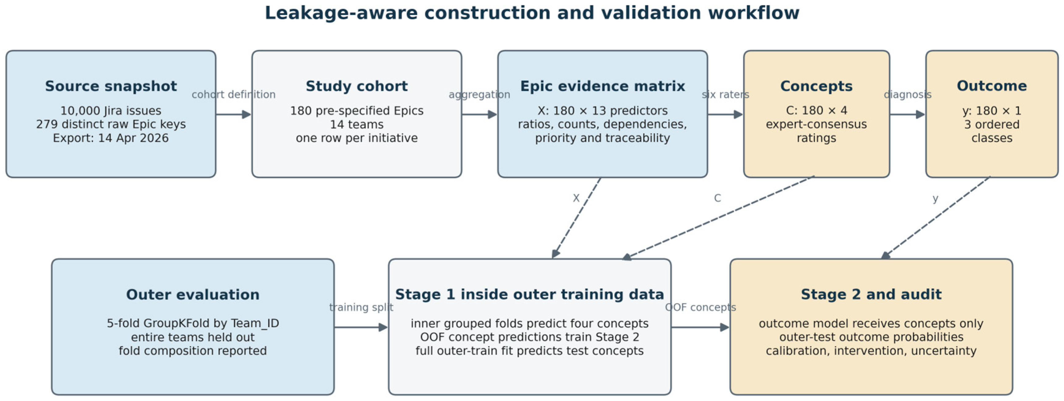
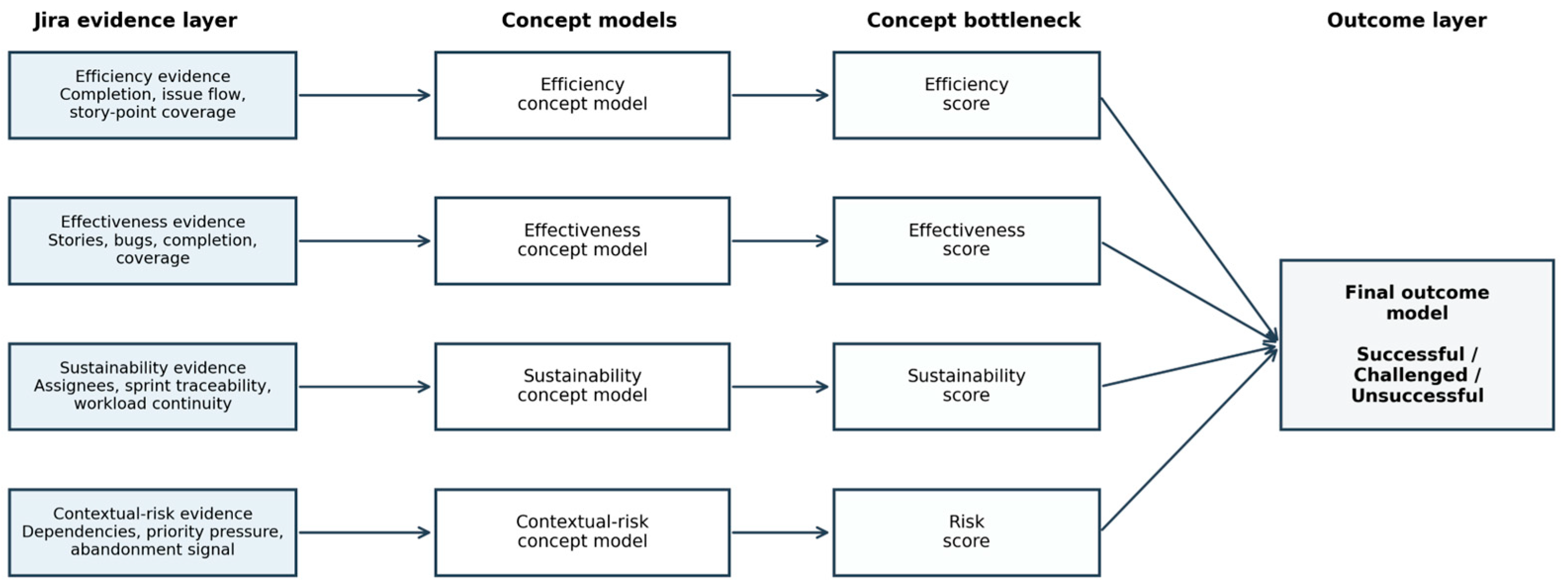
Figure 1 annotates the complete data and validation flow. The frozen export contains 10,000 unique Jira issues and 279 distinct raw Epic keys. The expert-review workbook defines the pre-specified study cohort of 180 Epics across 14 teams. Aggregation produces an evidence matrix X with 180 rows and 13 main predictors, a consensus concept matrix C with 180 rows and four columns, and one three-class outcome per Epic. Within each outer team-held-out fold, stage-one concept models generate inner out-of-fold predictions for second-stage training; outer-test concept predictions are produced only from models fitted to the corresponding outer-training data.

The remainder of this section describes each stage of Figure 1 in turn, beginning with the unit of analysis and the data source.

3.2. Unit of Analysis and Data Source

The unit of analysis is an Agile Epic, treated as a delivery initiative representing a coherent body of work. This level is more stable than an individual Jira issue for retrospective diagnosis; this is a domain-design choice, and not evidence that managers find the resulting explanations more useful.

The frozen Jira export dated 14 April 2026 contains 10,000 unique issue-level records and 279 distinct raw Epic keys. The reviewed evidence-and-rating workbook defines a pre-specified cohort of 180 Epics across 14 teams; the remaining raw Epic keys were outside that rating frame. The archived extraction materials do not contain a row-level exclusion-reason field for every non-cohort Epic, so the study reports the 279-to-180 provenance explicitly, rather than reconstructing undocumented criteria retrospectively. The analytical cohort contains the Jira evidence, expert ratings, and outcome records required for the reported analyses.

Two characteristics of

Table 2. Dataset characteristics.

Dataset Characteristic	Value
Source Jira issues in backup export	10,000
Epic-level observations retained	180
Distinct teams	14
Experts/raters	6
Outcome classes	Successful; Challenged; Unsuccessful
Jira export date	14 April 2026
Epics with explicit Last_Resolved_Date	76
Epics without explicit Last_Resolved_Date	104
Distinct raw Epic keys in source export	279

shape the analysis: the 10,000 issue records are the source snapshot, whereas 180 Epics are the effective supervised sample; and only 76 Epics have explicit resolution dates. All modelling claims, therefore, concern the frozen 180-Epic cohort, not the 279 raw Epic keys or the 10,000 individual issues.

3.3. Epic-Level Evidence Extraction and Censoring-Sensitive Variables

Table 3. Epic-level evidence features and use in analysis.

Feature	Definition	Source	Use
N_Issues	Total issues linked to the Epic	Jira issue count	Main model
N_Stories	Number of stories linked to the Epic	Jira issue type	Main model
N_Bugs	Number of bugs linked to the Epic	Jira issue type	Main model
Bug_Ratio	Proportion of Epic issues classified as bugs	Derived ratio	Main model
Completion_Ratio	Proportion of completed or resolved issues	Derived ratio	Main model
Abandoned_Ratio	Proportion of abandoned/cancelled/unresolved work	Derived ratio	Main model
SP_Total	Total story points attached to the Epic	Jira story points	Main model
SP_Completed	Completed story points	Jira story points/status	Main model
SP_Coverage	Completed story points divided by total story points	Derived ratio	Main model
Dependency_Count	Linked dependency relationships	Jira linked issues	Main model
N_Sprints_Touched	Number of sprints associated with the Epic	Jira sprint field	Main model, process-traceability indicator
N_Assignees	Number of distinct assignees	Jira assignee field	Main model
High-Priority_Ratio	Proportion of high-priority issues	Jira priority field	Main model
Duration_Days	Elapsed time when Last_Resolved_Date exists	Jira dates	Descriptive only; excluded from main prediction
Lead_Time_Mean/Median	Mean/median lead time for resolved issues	Jira dates	Descriptive only; excluded from main prediction

defines the main evidence features. Duration and lead-time variables are treated as censoring-sensitive because 104 of the 180 Epics did not have an explicit Last_Resolved_Date. Duration_Days and lead-time variables were retained for descriptive review, but excluded from the main predictive models. Completion_Ratio and Abandoned_Ratio remain process-state indicators and are therefore also interpreted cautiously: they support internal Jira-evidence classification, but may partially reflect whether an Epic was still active or poorly closed at the export date.

The final main predictive feature set, therefore, contains only non-censoring Jira evidence features. These features are not claimed to be independent business outcomes. Rather, they are observable Jira evidence used to assess how consistently outcome labels and diagnostic dimensions align with delivery traces.

For an Epic i, let N_i denote the number of linked issues, N_i(res) the number of resolved or completed issues, N_i(ab) the number of abandoned or cancelled issues, N_i(bug) the number of bug-type issues, SP_i(tot) the total story points, and SP_i(comp) the completed story points. The main derived ratio features are defined as

$${\text{Completion\_Ratio}}_i={\displaystyle \frac{N_i^{\mathrm{r}\mathrm{e}\mathrm{s}}}{N_i}}$$

(1)

$${\text{Abandoned\_Ratio}}_i={\displaystyle \frac{N_i^{\mathrm{a}\mathrm{b}}}{N_i}}$$

(2)

$${\text{Bug\_Ratio}}_i={\displaystyle \frac{N_i^{\mathrm{b}\mathrm{u}\mathrm{g}}}{N_i}}$$

(3)

$${\text{SP\_Coverage}}_i={\displaystyle \frac{S{P}_i^{\mathrm{c}\mathrm{o}\mathrm{m}\mathrm{p}}}{S{P}_i^{\mathrm{t}\mathrm{o}\mathrm{t}}}}$$

(4)

Ratio features improve cross-Epic comparability, while raw counts retain scale information but can introduce noise. Team-level inspection shows pronounced recording heterogeneity: most teams have a median SP_Total of zero, whereas team SQ has a median of 11.25, and median issue counts range from 5 to 32. Consequently, workload/scope ablation can improve performance because raw volume partly encodes team-specific Jira practice and initiative size, rather than delivery quality.

Two aspects of Table 3 matter for interpretation. First, the ratio features in Equations (1)–(4) are bounded in [0, 1], and are therefore comparable across Epics of very different sizes. Second, the explicit separation of censoring-sensitive temporal variables from the main feature set is a design decision, rather than an afterthought: it prevents the classifier from exploiting missing resolution dates as a shortcut signal for the Unsuccessful class.

3.4. Outcome Labelling, Circularity Risk, and Interpretation Boundary

Each Epic was assigned to one of three outcome classes: Successful, Challenged, or Unsuccessful. A Successful Epic refers to an initiative that achieved its intended delivery outcome with sufficient completion evidence. A Challenged Epic refers to partial completion, delay, dependency pressure, quality concerns, or unresolved delivery constraints. An Unsuccessful Epic refers to substantial non-completion, abandonment, or failure to achieve the intended outcome.

A central validity issue is circularity. Outcomes and concept ratings were derived retrospectively from overlapping Jira evidence. The fitted models therefore learn to reproduce an expert-informed labelling procedure; they do not establish independent project success, causal drivers, or prospective business value. High concept separability and perfect classification from true concept scores are treated as evidence of rubric coupling, not validation of real-world success.

The strongest way to remove this threat in future work would be to obtain outcome labels recorded before feature extraction or independent business outcomes such as realised value, sponsor acceptance, customer satisfaction, operational adoption, or post-release benefit realisation. In the present study, the limitation is mitigated, but not eliminated, by group-aware validation, censoring-sensitive feature exclusion, explicit concept-fidelity testing, case-level diagnostics, and transparent threats-to-validity reporting.

Table 4. Outcome class distribution.

Outcome Class	Count	Percent
Successful	41	22.8%
Challenged	81	45.0%
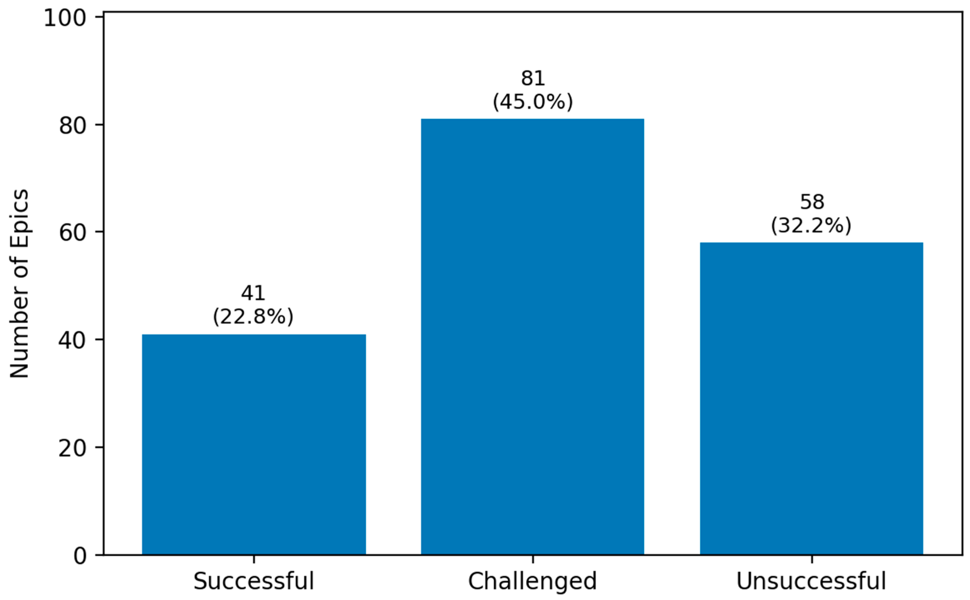
Unsuccessful	58	32.2%

and Figure 2 report the outcome distribution.

Table 4 and Figure 2 report the distribution of the three outcome classes in the labelled Epic-level dataset.

The class distribution in Table 4 and Figure 2 shows that Challenged Epics form the largest class, representing 45.0% of the dataset, followed by Unsuccessful Epics at 32.2% and Successful Epics at 22.8%. This distribution is not perfectly balanced, but it is sufficiently varied to support three-class classification. It also justifies the use of balanced accuracy and macro-F1 as headline evaluation metrics, because overall accuracy alone could overstate performance if a model favours the majority Challenged class.

The class distribution in Table 4 and Figure 2 has two direct methodological consequences. First, the Challenged class is the largest, at 45.0%, which fixes the majority-baseline accuracy at approximately 0.45 and provides a useful reference point for interpreting the later model comparison. Second, the imbalance motivates the emphasis on balanced accuracy and macro-F1 throughout the evaluation, because plain accuracy would reward models that over-predict the Challenged class.

3.5. Right-Censoring and Jira Process-Traceability Checks

Table 5. Explicit and missing resolution-date evidence by outcome class.

Outcome Class	Explicit Resolved Date	No Explicit Resolved Date
Challenged	42	39
Successful	24	17
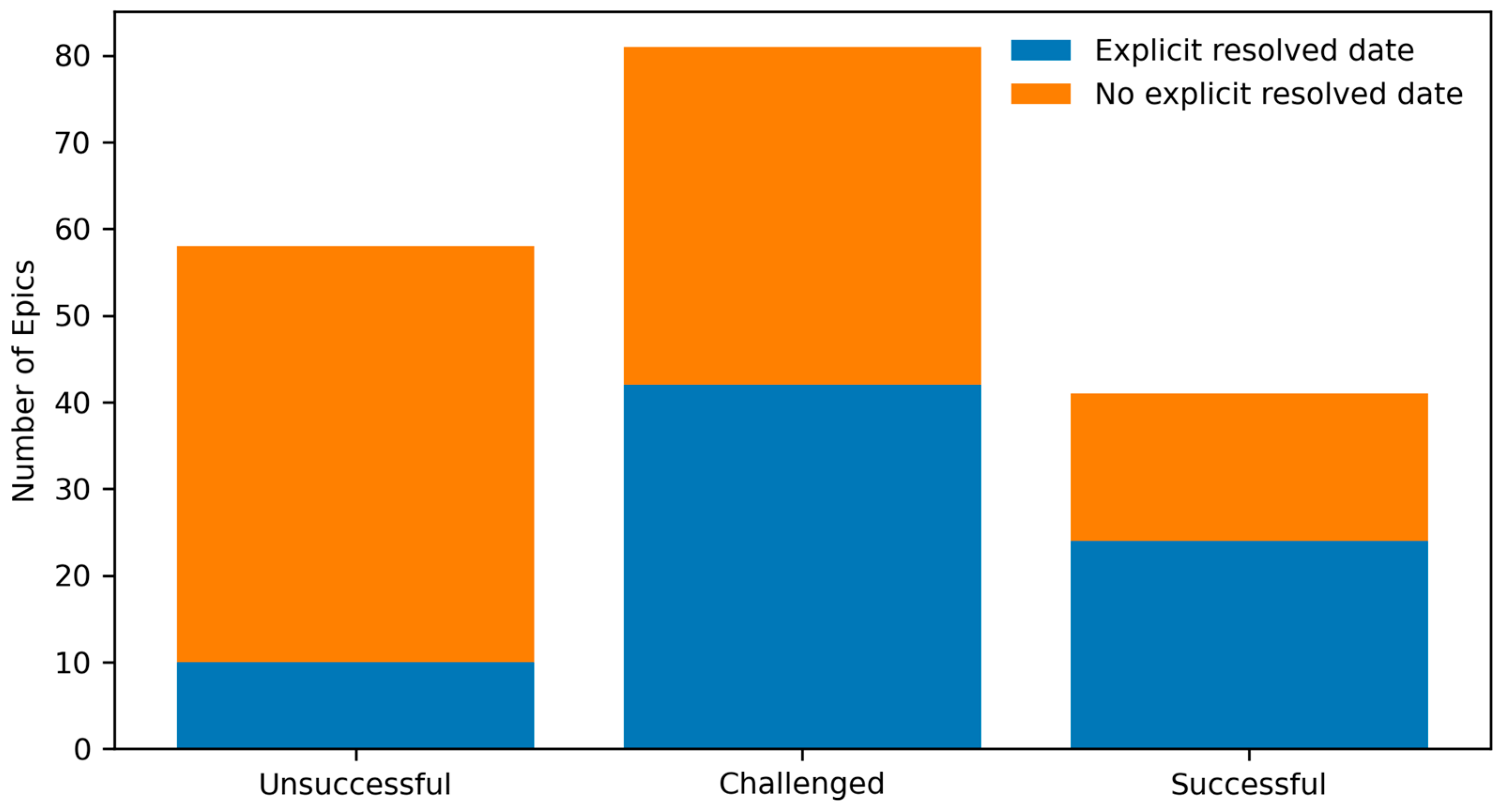
Unsuccessful	10	48

reports the class-specific distribution of explicit and missing resolution dates. A second validity issue is right-censoring and ambiguous process state. Of 180 Epics, 104 lack an explicit Last_Resolved_Date, including 48 of 58 labelled Unsuccessful. Missing closure can mean active work, deferral, weak Jira hygiene, or failure. Resolution-sensitive temporal variables were excluded from the primary feature set. A resolved-only analysis and a four-class Active/Unresolved sensitivity are reported; a survival model was not fitted because Jira resolution is a workflow-closure event, not an independently validated failure or success event, and the available snapshot does not establish a common observation origin or a stable event definition.

The dataset also revealed imperfect Jira process traceability. Mean N_Sprints_Touched and story-point coverage were low, indicating that not all Epics were consistently connected to sprint and estimation artefacts. This does not invalidate the study, but it narrows the claim: the findings concern Jira-supported Agile delivery diagnosis in a specific organisational data environment, not universal Agile maturity.

Figure 3 presents the same cross-tabulation graphically, highlighting how strongly missing resolution evidence concentrates in the Unsuccessful class.

The concentration of unresolved records in the Unsuccessful class is large: 48 of 58 Unsuccessful Epics (82.8%) lack an explicit resolution date, compared with 48.1% of Challenged and 41.5% of Successful Epics. This asymmetry makes perfect recall for Unsuccessful cases compatible with process-state shortcut learning. It is not interpreted as strong generalisation.

3.6. Expert Rating Procedure and Workload Controls

Six experts independently reviewed the Epic-level evidence and rated each Epic across four dimensions: efficiency, effectiveness, sustainability, and contextual risk. Efficiency, effectiveness, and sustainability were rated from 1 to 5, where 1 indicates very low or very poor performance and 5 indicates very high performance. Contextual risk was rated from 1 to 5 in the opposite direction, where 1 indicates low contextual risk and 5 indicates very high contextual risk. Experts also recorded confidence scores.

The expert panel was purposively assembled from practitioners with Agile delivery, product, portfolio, technical, or release-management experience. Each expert completed 720 dimension ratings (180 Epics × four dimensions) and 180 confidence scores, giving 900 quantitative judgements per rater and 5400 quantitative entries across the panel. The Epics were presented in a pseudonymised workbook with separate rater sheets and a shared rubric. Experts were instructed to work independently, to avoid discussion during the initial rating phase, and to use comments and confidence scores when evidence was ambiguous. No counterbalancing of Epic order was applied; therefore, order and fatigue effects remain possible and are treated as limitations.

Table 6. Expert-panel profile.

Expert ID	Role	Years	Sector Expertise	Independent from Epics
R1	Senior Agile Coach	12	FinTech/Telecom	Yes
R2	Scrum Master/Delivery Lead	8	Retail/Tech	Yes
R3	Product Portfolio Manager	10	Healthcare IT	Yes
R4	Lead Delivery Manager	15	E-commerce	Yes
R5	Technical Agile Practitioner	7	SaaS/Tech	Yes
R6	Release Train Engineer	14	Public Sector/Finance	Yes

summarises the expert panel.

The panel spans seven to fifteen years of experience across six different sector profiles, which reduces the risk that the ratings reflect a single delivery culture. At the same time, all six raters worked from the same Epic-level evidence table, so panel diversity mitigates rater-background bias but not the shared-evidence dependence discussed in Section 3.4.

3.7. Reliability, Concept Fidelity, and Diagnostic Separability

The rating task involved 4320 dimension scores plus confidence assessments. Experts used separate sheets, a shared rubric, and independent completion instructions. However, independence between raters does not make their evidence independent: all raters inspected the same Jira table. Reliability therefore measures consistent application of the rubric, not external confirmation of project success.

Formally, let x(i,d,r) denote the rating of Epic i on dimension d by rater r ∈ {1, …, R} with R = 6. The consensus concept score used in all subsequent analysis is the rater average:

$$c_{i,d}={\displaystyle \frac{1}{R}}{\displaystyle {\sum }_{r=1}^R}{x}_{i,d,r}$$

(5)

Reliability of these averaged scores was assessed with the two-way random-effects intraclass correlation for average measures [41]:

$$\mathrm{I}\mathrm{C}\mathrm{C}\left(2,k\right)={\displaystyle \frac{M{S}_R-M{S}_E}{M{S}_R+\left(M{S}_C-M{S}_E\right)/n}}$$

(6)

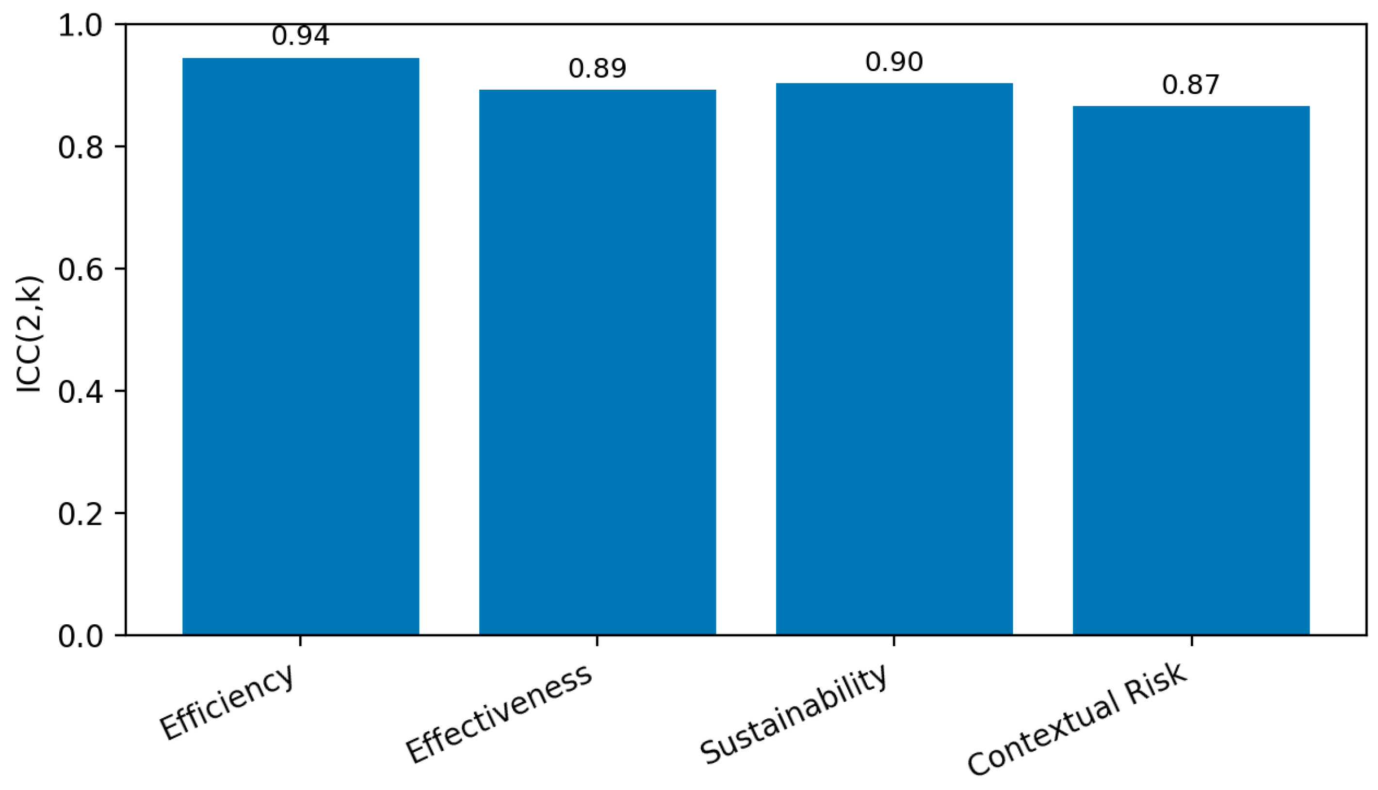
where MS_R, MS_C, and MS_E are the mean squares for rows (Epics), columns (raters), and error, respectively, and n is the number of Epics. Values above 0.75 are conventionally interpreted as good, and above 0.90 as excellent [41]. The resulting coefficients are reported in

Table 7. Inter-rater reliability for expert dimension ratings.

Dimension	ICC(2,k)	Interpretation
Efficiency	0.945	Excellent
Effectiveness	0.892	Good
Sustainability	0.902	Excellent
Contextual Risk	0.866	Good

.

RQ2 is evaluated without claiming user-validated interpretability. The validity audit includes concept fidelity, class separability, Spearman correlations, classification from true concepts as a coupling diagnostic, expert-rating dispersion, predictive uncertainty, probability calibration, and ±1-point concept interventions. These tests assess internal structure and failure modes; none demonstrates that practitioners make better decisions than with flat SHAP explanations.

Figure 4 visualises these coefficients: all four bars sit above the conventional 0.75 threshold for good reliability, and two exceed the 0.90 threshold for excellent reliability.

All four dimensions exceed the 0.85 level, with efficiency showing the highest agreement (0.945) and contextual risk the lowest (0.866). This ordering is plausible: efficiency can be anchored directly in completion and flow evidence, whereas contextual risk requires more inferential judgement about dependencies and environmental conditions, leaving more room for legitimate rater disagreement.

3.8. Threats to Validity and Safeguards

Table 8. Summary of validity threats and corresponding safeguards.

Threat	Risk	Safeguard/Interpretation Boundary
Label circularity	Outcome labels and concept ratings were evidence-informed	Results interpreted as internal evidence-aligned classification, not prospective independent prediction
Concept circularity	Experts rated concepts using the same evidence table	ICC interpreted as rubric consistency; concept fidelity and separability reported
Right-censoring	104 Epics lacked explicit Last_Resolved_Date	Duration and lead-time variables excluded from main models; resolved-subset check reported
Team-level leakage	Multiple Epics came from the same teams	5-fold group-aware cross-validation by Team_ID
Stacking leakage	Final model could see in-sample concept predictions	Out-of-fold concept predictions used inside the two-stage model
Class imbalance	Challenged class was the largest class	Balanced accuracy and macro-F1 reported alongside accuracy
Ordinal outcome structure	Successful > Challenged > Unsuccessful is ordered	Cumulative ordinal logistic baseline included
Ablation ambiguity	Features can map conceptually to multiple dimensions	Ablation uses mutually exclusive evidence families with exact removed features
Relationship to prior work	Previous collaborative Electronics article exists	Prior work cited and the distinct Jira/CBM-style diagnostic design is described
Interpretability claim	No practitioner user study was conducted	Interpretability framed as diagnostic structure; user validation listed as future work
Higher-level clustering	A product or project may span teams, but no separate Product_ID/Project_ID exists	Group by Team_ID; report the missing higher-level identifier and avoid cross-product generalisation claims.
Model selection optimism	Repeated inspection of five outer folds can bias fixed-config comparisons	Use restricted inner grouped selection and leave-one-team-out analyses as sensitivity checks; do not use them to rank LightGBM against HMXAI/CBM; outer-test teams remain untouched

summarises the main threats and the safeguards used. The wording is deliberately methodological, rather than defensive: the aim is to make the study boundary clear before interpreting the results.

Table 8 is intended as a reading guide for the results: each subsequent empirical section reports its findings against the corresponding interpretation boundary, so that predictive performance, concept fidelity, and diagnostic separability are each read with the correct scope of claim.

3.9. Predictive and Diagnostic Modelling Strategy

The main feature set excluded Duration_Days and lead-time variables because these fields were missing for many unresolved Epics and could encode censoring, rather than delivery quality. The models compared were a majority baseline, multinomial logistic regression, cumulative ordinal logistic regression, random forest, extra trees, flat LightGBM, and the HMXAI/CBM-style two-stage model.

The HMXAI/CBM-style model predicts four expert-consensus concepts and then predicts the outcome only from those concepts. In every outer fold, concept values used to train stage two are inner out-of-fold predictions: each training Epic is predicted by a stage-one model that excluded that Epic’s Team_ID fold. Stage-one models are then refitted on the complete outer-training set to predict concepts for the untouched outer-test teams. Neither full-dataset fitted concepts nor outer-test concept values enter stage-two training.

The two modelling strategies can be stated compactly. Let x_i denote the vector of the thirteen non-censoring evidence features for Epic i, and let y_i ∈ {Successful, Challenged, Unsuccessful}. The flat benchmark learns a direct mapping:

$${\widehat{y}}_i=h\left(x_i\right)$$

(7)

The HMXAI/CBM-style model instead decomposes the problem through the four Agile concepts. Stage one fits a separate regressor for each concept d ∈ {efficiency, effectiveness, sustainability, contextual risk}:

$${\widehat{c}}_{i,d}=g_d\left(x_i\right), d=1,\dots ,4$$

(8)

and stage two predicts the outcome only from the predicted concept vector, which is the bottleneck property that forces all evidence to pass through managerially recognisable diagnostic dimensions:

$${\widehat{y}}_i=f\left({\widehat{c}}_{i,1},{\widehat{c}}_{i,2},{\widehat{c}}_{i,3},{\widehat{c}}_{i,4}\right)$$

(9)

Because f receives only four concept predictions, rather than the full evidence vector, any outcome-relevant information that cannot be expressed through the concepts is discarded. This information compression is the theoretical mechanism behind the predictive trade-off observed in Section 4.2, and it is also what makes the concept layer diagnostically interpretable.

Figure 5 and Figure 1 distinguish two operations: inner out-of-fold concept generation for stage-two training and full outer-training refits for outer-test prediction. This procedure rules out stacking leakage at the Epic and Team_ID levels. It cannot rule out unobserved higher-level clustering because Project_ID/Product_ID was unavailable.

3.10. Evaluation Metrics and Statistical Comparison

Performance was evaluated using accuracy, balanced accuracy, macro-precision, macro-recall, macro-F1, and weighted-F1. The primary comparison used five-fold GroupKFold by Team_ID with configurations frozen in the accompanying code (random seed 42; scikit-learn 1.8.0; LightGBM 4.6.0). A restricted nested flat sensitivity analysis performed inner four-fold grouped model and hyperparameter selection within each outer-training split, comparing random forest, extra trees, and multinomial logistic candidates. A separate nested CBM diagnostic analysis tuned the four random-forest concept regressors and the stage-two logistic classifier. Neither flat LightGBM nor the primary fixed-configuration HMXAI/CBM model was included in a common inner-loop candidate set. These nested analyses are, therefore, model-specific optimism and diagnostic audits; they do not replace or rank the principal fixed-configuration results. Fold-specific teams and class counts appear in Appendix A.1 

Table A1. Outer-fold teams and class composition (Unsuccessful/Challenged/Successful).

Fold	Train n	Test n	Held-Out Teams	Class Counts
1	142	38	COL	12/22/4
2	143	37	ORGS	6/18/13
3	144	36	SQ	12/15/9
4	145	35	BD, IP, MR, QA, TES	17/12/6
5	146	34	AI, AT, DO, DS, ETB, PT	11/14/9

, and selected hyperparameters with outer-fold metrics appear in Appendix A.4 

Table A8. Selected hyperparameters and outer-fold results for the restricted nested flat sensitivity analysis.

Fold	Selected Model	Selected Hyperparameters	Inner Macro-F1	Outer Balanced Acc.	Outer Macro-F1
1	Random forest	n = 300; depth = None; leaf = 2; features = sqrt	0.844	0.912	0.834
2	Random forest	n = 100; depth = None; leaf = 5; features = sqrt	0.781	0.912	0.897
3	Random forest	n = 100; depth = 8; leaf = 2; features = sqrt	0.862	0.765	0.776
4	Extra trees	n = 300; depth = None; leaf = 2; features = sqrt	0.773	0.886	0.866
5	Random forest	n = 100; depth = None; leaf = 5; features = sqrt	0.813	0.800	0.796

Note: The inner candidate set also included multinomial logistic regression. Candidate-specific inner scores are archived in the Supplementary Results.

and

Table A9. Selected hyperparameters and outer-fold results for the separate nested CBM diagnostic sensitivity analysis.

Fold	Stage-One Depths (E/Ef/S/R)	Stage-Two C	Accuracy	Balanced Acc.	Macro-F1	Weighted-F1
1	6/None/6/6	1	0.842	0.909	0.805	0.863
2	None/6/None/None	10	0.919	0.930	0.933	0.918
3	None/6/None/6	0.1	0.972	0.978	0.971	0.972
4	None/None/None/None	10	0.943	0.917	0.917	0.943
5	None/None/6/6	10	0.824	0.817	0.816	0.820

Note: E/Ef/S/R denote efficiency, effectiveness, sustainability, and contextual risk. All selected stage-one regressors used 100 trees, max_features = 0.7, and min_samples_leaf = 2; only max_depth varied between 6 and unrestricted (None).

. Probability calibration is reported using multiclass Brier score, ten-bin expected calibration error (ECE), and log loss for the nested refits.

Preprocessing and candidate settings were fixed before inspecting each outer-test fold. Missing numeric values were median-imputed within the training data; standardisation was applied only to multinomial logistic regression. The primary random-forest and extra-trees classifiers used 50 trees, maximum depth 8, minimum leaf size 5, square-root feature sampling, balanced class weights, and random seed 42; LightGBM used 50 estimators, maximum depth 8, 31 leaves, learning rate 0.1, minimum child samples 10, and balanced class weights. The primary stage-one concept regressors used random forests with 50 trees, maximum depth 5, minimum leaf size 5, square-root feature sampling, and seed 42; the stage-two classifier was multinomial logistic regression with C = 1 and 1000 maximum iterations. Within the restricted nested flat inner loop, random forest and extra trees were compared over 100 or 300 trees, maximum depth unrestricted or 8, minimum leaf size 2 or 5, and square-root feature sampling; logistic regression used C in {0.1, 1, 10}. The separate nested CBM audit searched stage-one random forests over 100 or 300 trees, maximum depth unrestricted or 6, minimum leaf size 2 or 5, and max_features of 0.7 or square root, while stage-two logistic regression used C in {0.1, 1, 10}. All preprocessing objects and candidate-selection steps were fitted using outer-training data only. The outer-test teams remained completely untouched until the selected fold-specific pipeline was evaluated.

For K = 3 outcome classes, the two headline metrics are defined as

$$\mathrm{B}\mathrm{a}\mathrm{l}\mathrm{a}\mathrm{n}\mathrm{c}\mathrm{e}\mathrm{d} \mathrm{A}\mathrm{c}\mathrm{c}\mathrm{u}\mathrm{r}\mathrm{a}\mathrm{c}\mathrm{y}={\displaystyle \frac{1}{K}}{\displaystyle {\sum }_{k=1}^K}{\mathrm{R}\mathrm{e}\mathrm{c}\mathrm{a}\mathrm{l}\mathrm{l}}_k$$

(10)

$$\mathrm{Macro}\text{-}\mathrm{F}1={\displaystyle \frac{1}{K}}{\displaystyle {\sum }_{k=1}^K}{\displaystyle \frac{2\hspace{0.17em}{P}_k{R}_k}{P_k+R_k}}$$

(11)

where P_k and R_k denote the precision and recall of class k. Both metrics weight the three classes equally, so the minority Successful class contributes as much as the majority Challenged class.

To avoid overclaiming model differences from only five folds, the comparison between flat LightGBM and the HMXAI/CBM-style model used a paired discordant-error test on out-of-fold predictions. Fold-level significance testing was not used because only five cross-validation folds were available, which would provide very low inferential power. The discordant-error test is also interpreted cautiously, because the dataset is clustered and from a single organisation.

The paired comparison uses the exact binomial form of McNemar’s test [42]. With n10 Epics classified correctly by the flat model but not by the HMXAI/CBM-style model, n01 the reverse, and nd = n10 + n01 discordant pairs, the two-sided exact p-value is

$$p=2{\displaystyle {\sum }_{j=\max \left(n_{10},\hspace{0.17em}{n}_{01}\right)}^{n_d}}\left({\displaystyle \genfrac{}{}{0pt}{}{n_d}{j}}\right){\left({\displaystyle \frac{1}{2}}\right)}^{n_d}$$

(12)

With n10 = 9 and n01 = 5, Equation (12) yields p = 0.424, as reported in Section 4.3.

A unified notation summary is provided in

Table 9. Unified notation used in the methodology and evaluation.

Symbol	Definition
i	Epic index, i = 1, …, 180
j	Jira evidence-feature index, j = 1, …, 13
d	Concept index: efficiency, effectiveness, sustainability, contextual risk
r	Expert-rater index, r = 1, …, 6
X	Epic evidence matrix, 180 × 13
C	Expert-consensus concept matrix, 180 × 4
y_i	Ordered outcome code for Epic i: 0 Unsuccessful, 1 Challenged, 2 Successful
g_i	Team_ID grouping variable for Epic i
N_i	Number of Jira issues linked to Epic i
N_i(res), N_i(ab), N_i(bug)	Resolved/completed, abandoned/cancelled, and bug issue counts
SP_i	Story-point total or coverage quantity for Epic i
c_id, ĉ_id	Observed consensus rating and out-of-fold predicted concept
f_d(·)	Stage-one predictor for concept d
h(·)	Stage-two outcome classifier receiving predicted concepts only
K	Number of outcome classes, K = 3
P_k, R_k, F1_k	Precision, recall, and F1 for class k
n10, n01	Discordant correct/error counts in the paired exact test

.

4. Results

4.1. Descriptive Evidence Profile

Table 10. Descriptive statistics for non-censoring Jira evidence features.

Feature	Mean	SD	Min	Max
N_Issues	16.411	34.068	3.000	363.000
N_Stories	9.272	27.301	0.000	353.000
N_Bugs	1.144	4.472	0.000	48.000
Bug_Ratio	0.053	0.153	0.000	1.000
Completion_Ratio	0.585	0.402	0.000	1.000
Abandoned_Ratio	0.068	0.143	0.000	1.000
SP_Total	6.075	15.207	0.000	101.000
SP_Completed	4.731	13.425	0.000	101.000
SP_Coverage	0.168	0.326	0.000	1.000
Dependency_Count	2.050	3.857	0.000	24.000
N_Sprints_Touched	0.439	1.532	0.000	14.000
N_Assignees	2.728	2.695	0.000	15.000
High-Priority_Ratio	0.131	0.268	0.000	1.000

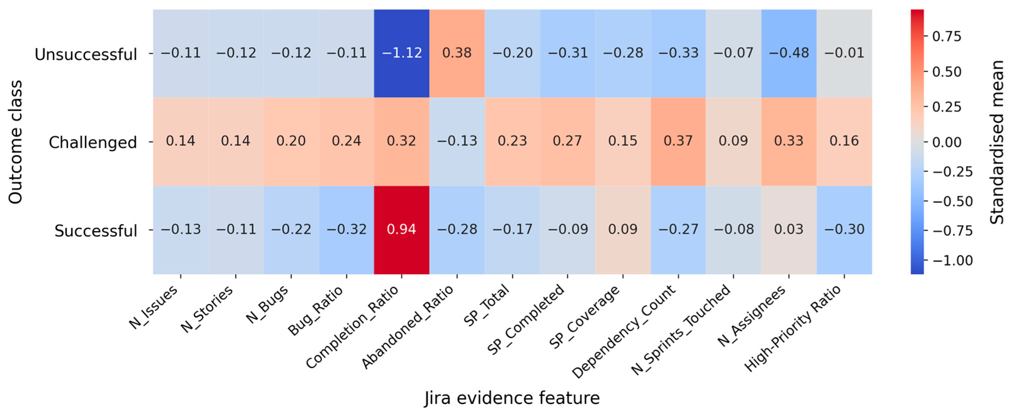
reports selected descriptive statistics for the non-censoring evidence features used in the main models. The data show substantial variation in completion behaviour, abandonment, dependency count, workload, and priority mix. Figure 6 further shows that outcome classes have distinct standardised Jira evidence profiles.

The distributions in Table 10 are strongly right-skewed: N_Issues has a mean of 16.4 but a maximum of 363, and story-point totals show similarly heavy tails. Tree-based models are well suited to such skewed, mixed-scale inputs, which partly explains their advantage over the linear baselines in

Table 11. Fixed-configuration predictive-model comparison using five-fold group-aware cross-validation.

Model	Accuracy	Balanced Accuracy	Macro-F1	Weighted-F1
Majority baseline	0.447 ± 0.089	0.333 ± 0.000	0.205 ± 0.028	0.281 ± 0.095
Logistic regression	0.706 ± 0.116	0.739 ± 0.086	0.694 ± 0.099	0.701 ± 0.114
Ordinal logistic (cumulative)	0.740 ± 0.075	0.780 ± 0.035	0.721 ± 0.061	0.727 ± 0.076
Random forest	0.878 ± 0.047	0.890 ± 0.043	0.870 ± 0.058	0.881 ± 0.043
Extra trees	0.796 ± 0.052	0.820 ± 0.060	0.785 ± 0.061	0.793 ± 0.053
LightGBM flat	0.879 ± 0.054	0.891 ± 0.028	0.864 ± 0.053	0.883 ± 0.050
HMXAI/CBM-style two-stage	0.857 ± 0.080	0.870 ± 0.050	0.843 ± 0.084	0.861 ± 0.074

, while the low means of N_Sprints_Touched (0.44) and SP_Coverage (0.17) quantify the process-traceability limitation discussed in Section 3.5. Figure 6 complements these statistics by standardising each feature within outcome classes.

Figure 6 shows an interpretable ordering: Successful Epics combine high completion with low abandonment, bug exposure, and priority pressure; Unsuccessful Epics show the inverse profile; and Challenged Epics carry the heaviest workload and dependency load, indicating that they are frequently large, complex delivery packages, rather than simply failed ones. This last pattern matters managerially, because it suggests that the Challenged class is partly a scale-and-coordination phenomenon, rather than purely a performance deficit.

4.2. Model Comparison

Table 11 reports the primary fixed-configuration comparison under five-fold Team_ID-grouped cross-validation. Random forest and LightGBM had the highest fold-mean scores within this evaluated fixed-configuration candidate set. The HMXAI/CBM-style model had a lower mean macro-F1 (0.843 ± 0.084) than flat LightGBM (0.864 ± 0.053) and random forest (0.870 ± 0.058). This descriptive comparison does not constitute joint nested-model selection; within the frozen configurations and sample evaluated, the hierarchy did not improve predictive performance.

Three observations follow from Table 11. First, the higher-scoring fixed-configuration flat candidates are close to each other, so the result applies only to this sample and the configurations evaluated here. Second, the concept hierarchy trades predictive freedom for a four-dimensional bottleneck. Third, the diagnostic structure cannot be treated as actionable merely because its labels are recognisable; intervention and user validation are separate requirements. The restricted nested-flat and separate nested-CBM sensitivities reported in Appendix A are not a common selection procedure and must not be used to extend the ranking in Table 11.

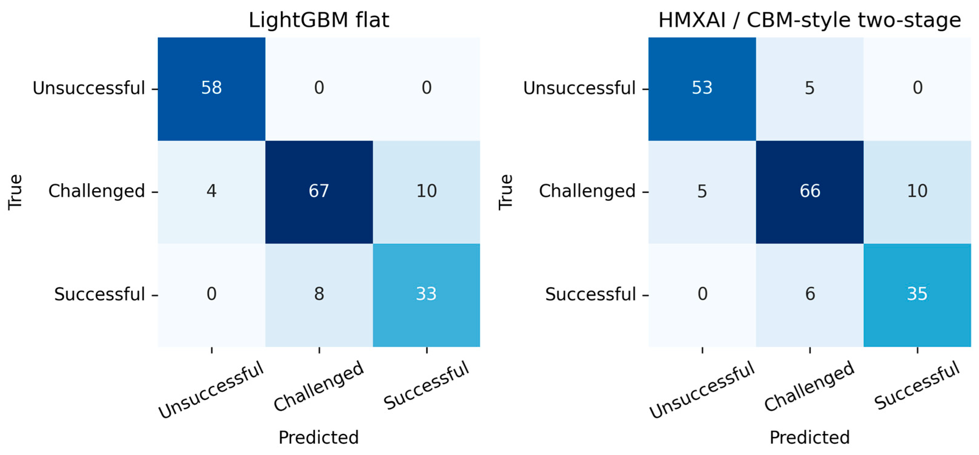
Class-level behaviour is shown in Figure 7. LightGBM predicts all 58 Unsuccessful Epics correctly, but 48 of those 58 lack resolution dates. The perfect recall is therefore consistent with reliance on completion and unresolved-state evidence, and is not presented as a feature of operational safety or strong external generalisation.

Figure 7 shows that the models share the same correct-or-incorrect verdict on 166 of 180 Epics, leaving only 14 discordant cases. This descriptive overlap does not establish equivalence, superiority, or deployment safety.

4.3. Statistical Comparison, Resolved-Subset Sensitivity, and Interpretation of Predictive Claims

Table 12. Paired discordant-error comparison of flat LightGBM and HMXAI/CBM-style model.

Comparison	Flat Correct/HMXAI Wrong	Flat Wrong/HMXAI Correct	Discordant Pairs	Exact p-Value	Interpretation
LightGBM flat vs. HMXAI	9	5	14	0.424	Underpowered; no statistically reliable difference

reports the paired discordant-error comparison. In the primary fixed-configuration analysis, flat LightGBM had the higher mean macro-F1. In the pooled out-of-fold predictions, LightGBM was correct for nine Epics and the HMXAI/CBM-style model was wrong for nine Epics, while the reverse occurred for five; the exact paired p-value was 0.424. With only 14 discordant pairs, the test has low power, and cannot establish equivalence or operational competitiveness. It simply fails to detect a directional difference in this sample, and must not be interpreted as a nested-model-selection result.

The conservative conclusion is therefore limited to the evaluated fixed configurations: the proposed hierarchy did not improve upon the higher-scoring flat candidates in this sample. Its remaining research value is the inspectable four-concept structure, subject to the coupling, uncertainty, intervention, and user-validation limitations reported below.

An exploratory sample-size extrapolation evaluates a hypothetical 1000-Epic sample without asserting equivalence. If the current discordance rate and 9:5 asymmetry persisted independently, approximately 78 discordant pairs (50 versus 28) would be expected at n = 1000, giving an exact p-value near 0.017 and approximate power of 0.65. This calculation ignores team clustering and assumes stable error rates, so it shows only that a larger sample could make the present small difference statistically detectable; it does not predict the substantive ordering of future models.

Because missing resolution evidence is unevenly distributed,

Table 13. Resolved-subset sensitivity check.

Model	n	Outcome Distribution	Balanced Accuracy	Macro-F1
LightGBM flat (full sample)	180	Successful = 41; Challenged = 81; Unsuccessful = 58	0.891 ± 0.028	0.864 ± 0.053
LightGBM flat (resolved subset)	76	Challenged = 42; Successful = 24; Unsuccessful = 10	0.689 ± 0.247	0.645 ± 0.244
Random forest (resolved subset)	76	Challenged = 42; Successful = 24; Unsuccessful = 10	0.735 ± 0.204	0.714 ± 0.200
HMXAI/CBM-style two-stage (resolved subset)	76	Challenged = 42; Successful = 24; Unsuccessful = 10	0.666 ± 0.110	0.540 ± 0.138

reports the resolved-only sensitivity. Appendix A.3 

Table A6. Active/Unresolved and process-state shortcut sensitivities.

Analysis	Accuracy	Balanced Acc.	Macro-F1
Four-class sensitivity: Active/Unresolved as class (all features)	0.417	0.306	0.305
Four-class sensitivity without completion/abandonment	0.439	0.211	0.202
Three-class shortcut diagnostic using completion/abandonment only	0.767	0.791	0.766

additionally treats all 104 records without a resolution date as an Active/Unresolved class. This four-class formulation is deliberately diagnostic: it separates process state from resolved outcome, but leaves only 10 resolved Unsuccessful cases.

Resolved-only results are substantially weaker and more variable. The four-class Active/Unresolved analysis is also weak (macro-F1 = 0.305 with all features and 0.202 without completion/abandonment), showing that an explicit Active class does not rescue outcome generalisation in this snapshot. A survival endpoint was not constructed because resolution is not an independently validated failure event.

The drop is material, rather than minor: LightGBM macro-F1 falls by approximately 0.22, from 0.864 to 0.645, on the 76 resolved Epics; the HMXAI/CBM-style model falls to 0.540. These values, together with 0.766 macro-F1 from Completion_Ratio and Abandoned_Ratio alone, show strong dependence on process-state variables.

4.4. Concept Fidelity and Diagnostic Separability

Table 14. Concept fidelity: predicting expert-consensus concepts from Jira evidence.

Concept	R2	MAE
Contextual Risk	0.678 ± 0.072	0.437 ± 0.062
Effectiveness	0.656 ± 0.097	0.408 ± 0.038
Efficiency	0.773 ± 0.052	0.412 ± 0.070
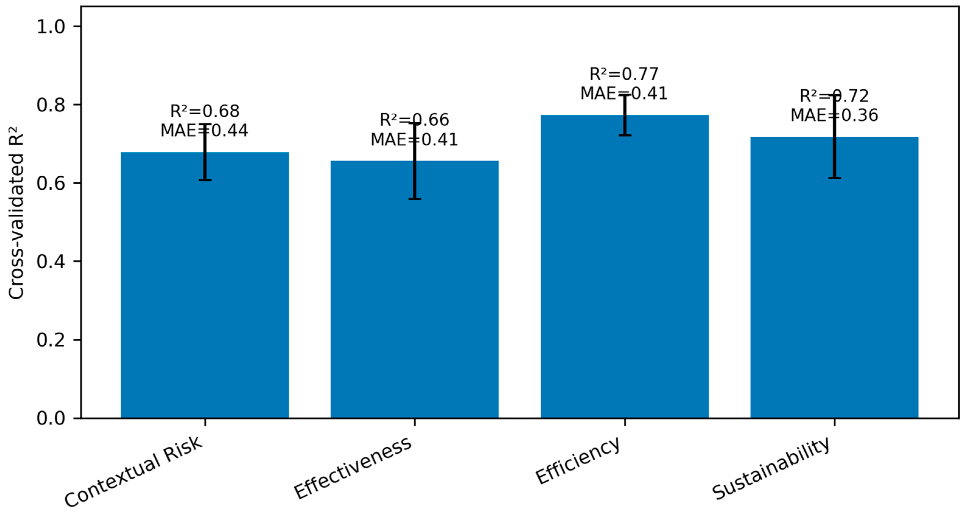
Sustainability	0.717 ± 0.106	0.362 ± 0.060

and Figure 8 report primary concept fidelity. Appendix A 

Table A2. Grouped sensitivity and calibration summary.

Analysis	Selection/Estimator	Macro-F1	Balanced Acc.	Brier	ECE
Primary flat LightGBM	Fixed configuration; not nested-tuned	0.864 ± 0.053	0.891 ± 0.028	Not archived	Not archived
Primary HMXAI/CBM	Fixed configuration; not nested-tuned	0.843 ± 0.084	0.870 ± 0.050	Not archived	Not archived
Restricted nested flat sensitivity	Inner grouped: logistic, RF, ET only	0.840	0.839	0.274	0.163
Separate nested CBM diagnostic audit	RF concepts + tuned logistic stage 2	0.894	0.902	0.168	0.051
Leave-one-team-out RF	14 held-out-team folds	0.821	0.812	—	—

,

Table A3. Spearman correlations among expert-consensus concepts.

Concept	Efficiency	Effectiveness	Sustainability	Contextual_Risk
Efficiency	1.000	0.842	0.857	−0.869
Effectiveness	0.842	1.000	0.833	−0.846
Sustainability	0.857	0.833	1.000	−0.843
Contextual_Risk	−0.869	−0.846	−0.843	1.000

,

Table A4. ±1-point concept intervention audit.

Concept	Direction	Class Changed	Mean Δ Expected Class	Expected Monotonicity
Contextual_Risk	decrease	14.4%	+0.154	93.3%
Contextual_Risk	increase	10.0%	−0.121	93.3%
Effectiveness	decrease	17.8%	−0.129	81.1%
Effectiveness	increase	20.0%	+0.157	78.3%
Efficiency	decrease	15.0%	−0.170	100.0%
Efficiency	increase	21.1%	+0.226	100.0%
Sustainability	decrease	8.3%	−0.042	82.8%
Sustainability	increase	16.1%	+0.112	78.3%

and

Table A5. Tree-ensemble concept-layer predictive uncertainty.

Concept	Mean Predictive SD	Mean 90% Interval Width	Empirical Coverage
Contextual_Risk	0.426	1.294	73.3%
Effectiveness	0.411	1.262	78.9%
Efficiency	0.450	1.341	80.0%
Sustainability	0.376	1.110	77.2%

extend the audit with calibration, concept correlation, expert-rating dispersion, predictive uncertainty, true-concept coupling, and manual interventions. These analyses test whether the bottleneck behaves coherently; they do not validate independent project success.

The fidelity ordering is informative. Efficiency is the most learnable concept (R² = 0.773), consistent with its direct grounding in completion and flow evidence, whereas effectiveness is the least learnable (R² = 0.656), reflecting that value judgements are only partially visible in process traces. All four mean absolute errors are below 0.44 on the five-point scale, meaning the concept models recover expert consensus to within roughly half a rating point, which supports the usability of the concept layer defined in Equation (8).

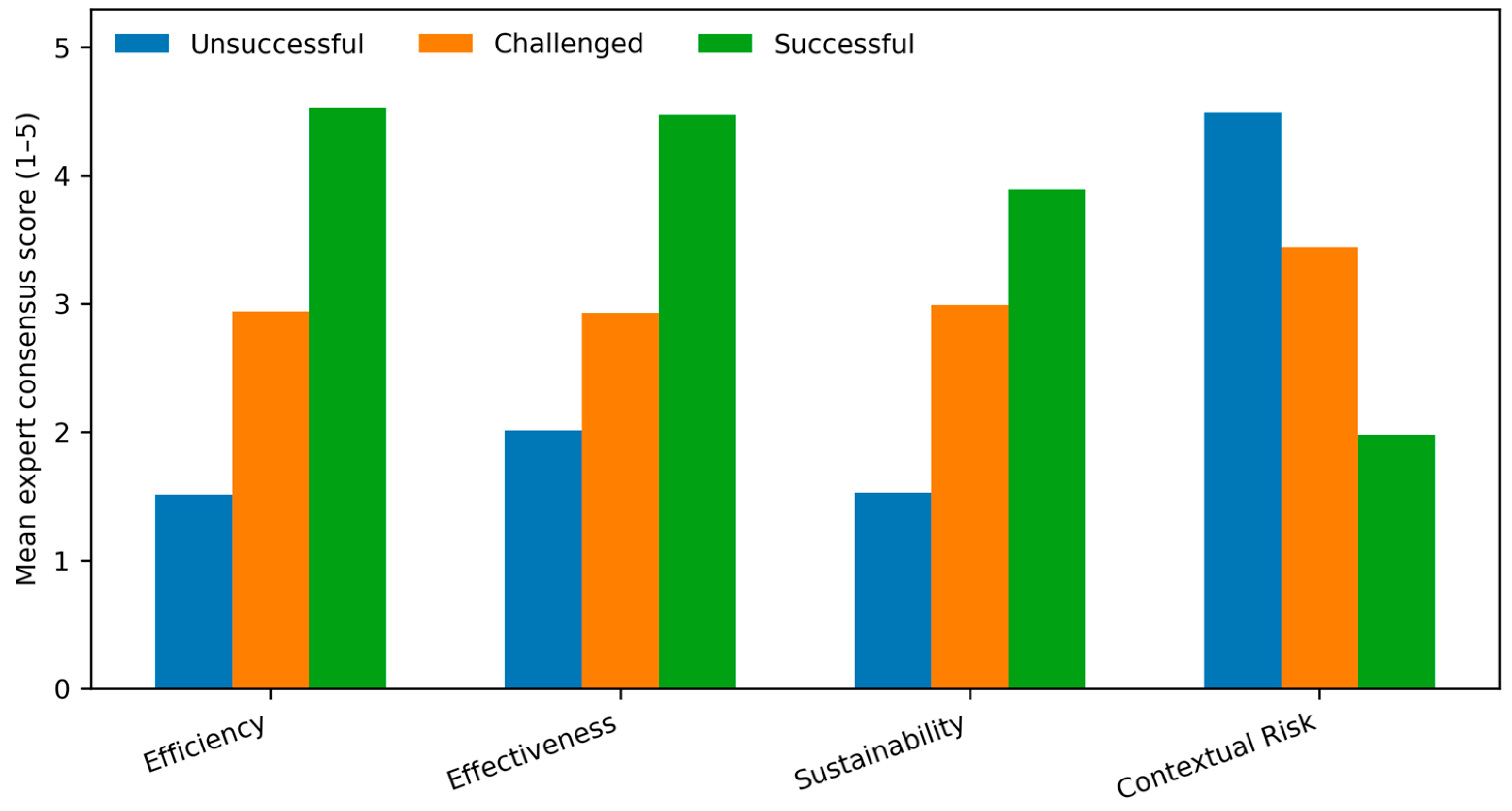
All four consensus concepts differ strongly across outcome classes, but this separability is structurally coupled to the labelling process. A grouped classifier using the four true consensus concepts reproduces all 180 labels (macro-F1 = 1.000). The result is reported as concept-label leakage/coupling, not as meaningful diagnosis.

Effect sizes in

Table 15. Diagnostic separability of expert-consensus dimensions by outcome class.

Dimension	Kruskal H	p-Value	Epsilon-Squared
Efficiency	155.44	<0.001	0.867
Effectiveness	151.00	<0.001	0.842
Sustainability	151.69	<0.001	0.846
Contextual Risk	150.94	<0.001	0.841

use the epsilon-squared statistic for the Kruskal–Wallis H test:

$${\epsilon }^2={\displaystyle \frac{H}{\left(n^2-1\right)/\left(n+1\right)}}$$

(13)

The observed H values and large epsilon-squared statistics indicate a highly consistent ordinal rubric. Spearman correlations are also high: the three positive concepts correlate at 0.833–0.857, and their correlations with contextual risk range from −0.843 to −0.869. The concept layer is therefore not four independent channels.

Figure 9 displays the consensus profiles by outcome. Their ordered appearance is expected from the shared evidence-and-rubric construction and should not be interpreted causally.

Manual ±1-point interventions in the nested CBM audit changed the predicted class for 8.3–21.1% of Epics, depending on concept and direction. Expected monotonicity was complete for efficiency, but only 78.3–81.1% for effectiveness, 78.3–82.8% for sustainability, and 93.3% for contextual risk. Non-monotone cases directly limit the claim that concept changes map reliably to managerial interventions.

4.5. Evidence-Family Ablation with Explicit Feature Groups

The ablation analysis uses mutually exclusive evidence families and reports the exact removed features in

Table 16. Evidence-family ablation with exact features removed.

Feature Set	Features Removed	Macro-F1	Balanced Accuracy
All non-censoring evidence features	None	0.864 ± 0.053	0.891 ± 0.028
Without Completion/abandonment	Completion_Ratio, Abandoned_Ratio	0.519 ± 0.087	0.542 ± 0.077
Without Defect/quality	N_Bugs, Bug_Ratio	0.788 ± 0.066	0.821 ± 0.061
Without Workload/scope	N_Issues, N_Stories, SP_Total, SP_Completed, SP_Coverage	0.878 ± 0.055	0.909 ± 0.035
Without Coordination/priority	Dependency_Count, N_Sprints_Touched, N_Assignees, High_Priority_Ratio	0.854 ± 0.035	0.880 ± 0.037

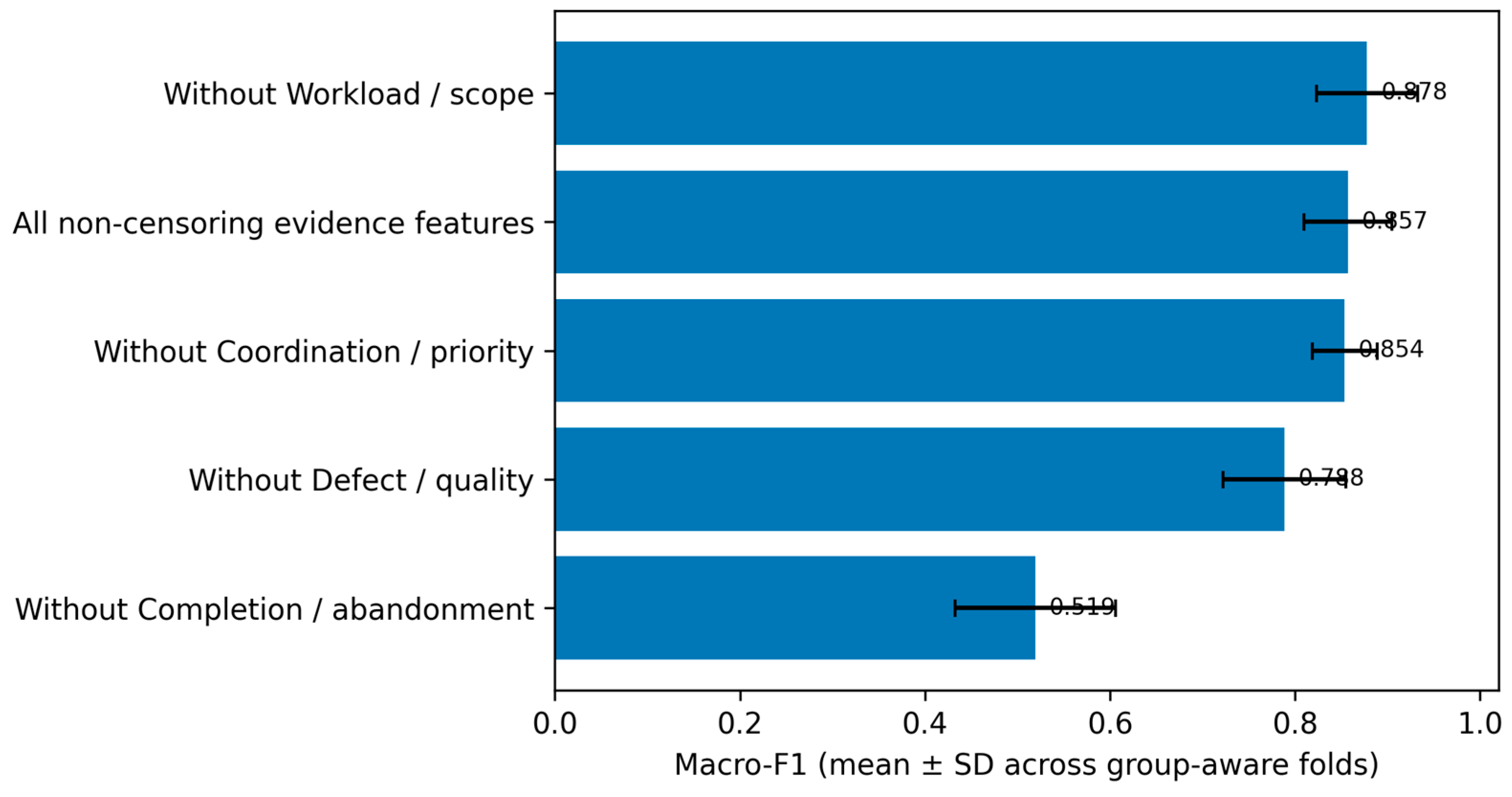
. Figure 10 visualises the results. The all-feature row is aligned with the LightGBM configuration reported in Table 11, to avoid mixing baselines from different pipelines.

Removing completion and abandonment produces the largest loss, confirming that the classifier relies on Jira process state. Conversely, removing workload/scope slightly improves macro-F1. This is plausible because story-point use is highly team-specific and mostly zero outside team SQ, while issue volume varies sharply by team and Epic size. Raw volume can therefore add local workflow noise without adding independent outcome information.

The ablation is a warning, rather than a deployment recommendation: reliable closure fields can improve reproduction of retrospective labels, but the same fields can create shortcut learning when outcome definitions and unresolved status overlap.

4.6. SHAP-Based Feature Explanation

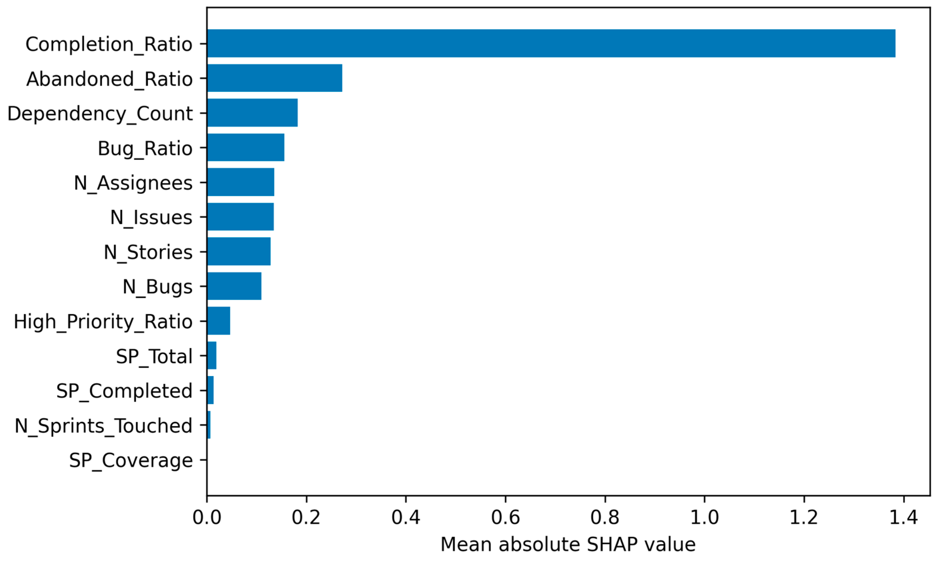
Figure 11 presents global SHAP importance for flat LightGBM. Completion_Ratio and Abandoned_Ratio dominate, followed by dependency, bug, assignee, and volume measures. Because the outcome and concepts were derived from overlapping evidence, SHAP identifies fields used to reproduce the labelling procedure; it does not identify causal drivers of independent business success.

SHAP attributes each prediction to features using Shapley values from cooperative game theory [16]. For feature j within the feature set F, the attribution is

$${\varphi }_j={\sum }_{S\subseteq F\setminus \left\{j\right\}}{\displaystyle \frac{\left|S\right|!\hspace{0.17em}\left(\left|F\right|-\left|S\right|-1\right)!}{\left|F\right|!}}\left[v\left(S\cup \left\{j\right\}\right)-v\left(S\right)\right]$$

(14)

where v(S) denotes the model output when only the feature subset S is available. The global importance in Figure 11 aggregates the absolute attributions |φ_j| across all Epics.

The SHAP ranking and concept mapping provide two description levels, but neither has been compared in a practitioner decision study. They should be described as feature-level and domain-labelled diagnostic summaries, not as proven managerial explanations.

4.7. Illustrative Case-Level Diagnostic Vignettes

Table 17. Illustrative diagnostic vignettes.

Epic	Outcome	Selected Jira Evidence	Concept Profile	Diagnostic Interpretation
AT−56	Successful	Comp. 1.00; Aband. 0.00; Bug 0.00; Dep. 1	Eff 4.50; Val 4.83; Sust 4.00; Risk 2.33	High completion; low abandonment; strong efficiency/effectiveness; moderate contextual risk.
ETB−121	Challenged	Comp. 0.95; Aband. 0.05; Bug 0.03; Dep. 24	Eff 3.17; Val 3.17; Sust 3.17; Risk 3.67	Large workload and high-dependency exposure; high completion but dependency pressure and residual risk.
ETB−116	Unsuccessful	Comp. 0.00; Aband. 1.00; Bug 0.00; Dep. 0	Eff 1.67; Val 1.83; Sust 1.50; Risk 4.33	No completion evidence and full abandonment; low concept scores and high contextual risk.

provides illustrative vignettes of the output format. These cases demonstrate presentation structure only; they do not show that managers make better, faster, or safer decisions than with flat SHAP explanations.

The three vignettes illustrate three distinct archetypes that a single flat risk score would collapse into one number: a clean success (AT-56); a complexity-loaded challenge in which delivery was largely completed but 24 dependency links were kept risk elevated (ETB-121); and an abandonment-driven failure with no completion evidence (ETB-116). Each archetype implies a different first intervention—none, dependency management, and scope or investment review, respectively—which is precisely the discrimination the concept layer is designed to support.

5. Discussion

5.1. Theoretical Implications

The findings support a multidimensional representation of retrospective Agile delivery states, but they also expose the boundary between representation and validation. Completion, abandonment, defects, dependencies, and workload distinguish the expert-labelled classes, while the four-concept bottleneck compresses those fields into a domain-labelled structure. The compression is inspectable, yet highly correlated concepts and perfect outcome reconstruction from true concept scores show that the bottleneck mirrors the rubric closely.

Within the primary fixed-configuration analysis, the HMXAI/CBM-style model did not improve upon the higher-scoring flat candidates in this sample. Its contribution is therefore architectural and diagnostic: it makes the intermediate assumptions visible and permits fidelity, uncertainty, correlation, leakage, and intervention audits. The intervention audit shows that recognisable labels do not guarantee monotone or actionable behaviour. No claim is made that the restricted nested analyses rank LightGBM against HMXAI/CBM.

The validation results also show why high accuracy is insufficient. The restricted nested flat selection and leave-one-team-out sensitivity produced lower pooled scores than the strongest fixed-configuration flat models, resolved-only performance fell sharply, and two process-state ratios alone remained strongly predictive. The separately tuned nested CBM score is treated only as a diagnostic sensitivity, because it was not selected in the same inner-loop candidate set as LightGBM. Together these findings are consistent with local Jira shortcut learning, and limit claims beyond the frozen organisation.

5.2. Managerial Implications

Practically, the models should be treated as retrospective audit aids, not autonomous success predictors. A flat model can summarise similarity to historical labels, and the concept layer can organise that summary into four rubric dimensions. Neither output has been shown to improve practitioner decisions, and any use requires review of the underlying Jira evidence.

Completion and abandonment warrant special caution. They are informative indicators of workflow state, but overlap with how Successful and Unsuccessful labels were judged. A high-risk flag based on these fields should trigger verification of whether work is genuinely failed, still active, intentionally deferred, or simply poorly closed in Jira.

The workload ablation highlights data-governance heterogeneity. Story-point totals are zero for most teams and issue volumes vary substantially, so cross-team comparisons require standardised estimation, Epic linking, sprint association, and closure practices before modelling.

A defensible workflow is therefore evidence-first based: inspect the Epic record, distinguish active from resolved work, review the concept profile with its uncertainty, and document any decision separately from the model output. The present study does not validate thresholds, interventions, or user benefit.

Any deployment would require independent outcome definitions, prospective monitoring, probability calibration in the target environment, drift checks, appeal and override procedures, and a practitioner study comparing flat and concept-based explanations.

5.3. Relationship to Previous Work

Relative to prior Agile prediction work [15], the present study adds a concept bottleneck and a broader validity audit. The supervised and unsupervised engineering studies [34,35] demonstrate domain-informed representation and transfer, while the cross-site forecasting study [36] illustrates external-site evaluation. Their data and targets differ, so they inform validation design, rather than numerical benchmarking.

The XAI study [39] applies SHAP and LIME to field data, but does not report a controlled practitioner-decision experiment. It is therefore treated as a domain-specific explanation example, rather than evidence of end-user validation.

5.4. Ethical, Reproducibility, and Data-Governance Considerations

The study uses anonymised operational records and pseudonymised expert profiles. The main ethical risk is not personal identification alone; it is overinterpreting workflow data as business success and using correlated process states to rank teams or individuals. The manuscript therefore restricts the target to retrospective evidence-aligned diagnosis.

Raw Jira data cannot be released because of organisational confidentiality. The Supplementary Materials (Files S1–S3) provide path-agnostic analysis scripts, the frozen schema, a synthetic execution example, aggregate outputs, fold composition, model-specific nested sensitivity outputs, intervention and uncertainty summaries, an environment/dependency record, and file-integrity manifests. Confidential row-level records and predictions are excluded. The original fitted binaries and exact original SHAP package version were not archived, and are therefore unavailable. The synthetic example verifies pipeline execution but cannot reproduce the reported estimates. Comparisons are limited to the evaluated candidates, and must distinguish fixed-configuration primary results from the restricted, non-joint nested sensitivity analyses.

6. Conclusions, Limitations, and Future Work

This study evaluates a concept-bottleneck-style architecture for retrospective diagnosis of Agile Epic labels from Jira evidence. Flat LightGBM had a higher mean macro-F1 than the primary HMXAI/CBM-style model under the evaluated fixed configurations; this descriptive result is not a joint nested-model-selection comparison. The contribution is therefore not predictive superiority, but an explicit diagnostic bottleneck and an audit showing where that structure succeeds and fails.

The evidence supports a narrower claim: the labels and concepts reproduce a shared expert rubric; unresolved state and completion/abandonment dominate; resolved-only and leave-one-team-out results are weaker; the four concepts are strongly correlated; true concepts reconstruct the labels perfectly; and interventions are not uniformly monotone. The model therefore diagnoses evidence-aligned process states, rather than independent project success.

Generalisability is limited by one organisation, 180 Epics, 14 uneven teams, no separate project/product grouping identifier, retrospective shared-evidence labelling, and absent practitioner evaluation. Runtime and calibration are reported for model-specific nested refits, but LightGBM and the primary HMXAI/CBM model were not tuned and selected within one commensurate inner-loop candidate set. The original fitted binaries and SHAP environment were not archived. These limitations prevent claims of causal explanation, comparative superiority under joint tuning, equivalence, safety, or proven actionability.

Future work should use prospectively recorded independent outcomes, multi-organisation and cross-product validation, explicit active-state or valid time-to-event designs, larger team-balanced cohorts, calibrated uncertainty, monotonic or causally constrained concepts, and controlled studies comparing concept-based explanations with flat SHAP. The current framework is best viewed as a transparent research prototype for auditing retrospective Jira diagnoses.