Bose–Fermi Mapping in Hubbard Models at Imaginary Chemical Potential and Phase-Induced Fermionization

Abstract

A formal thermodynamic mapping is established between the attractive Fermi–Hubbard model and the repulsive Bose–Hubbard model at finite temperature and at imaginary chemical potential $\mu =i\theta$. By utilizing a large N-expansion, it is shown that the partition functions of the two models are related by a plain shift $\theta \to \theta +\pi$. This condition maps the BCS–BEC crossover of attractive fermions to a Bose–Fermi crossover (fermion-like occupation) of repulsive bosons. A central feature of this correspondence is the thermal kernel $g(\beta E,\varphi )$ (with $\beta$ the inverse absolute temperature, E the energy scale, and $\varphi$ the phase angle), whose analytic continuation $g_B(\beta E,\varphi )=g_F(\beta E,\varphi +\pi )$ governs the bosonic (B) and fermionic (F) sectors. Interestingly, the particular angles $\varphi =2\pi /3$ and $4\pi /3$ for fermions correspond to $\varphi =\pi /3$ and $5\pi /3$ for bosons, marking the boundaries of an universal thermal window. It is further argued that the present mechanism shows how an emergent, fermionization-like phenomenon can occur at finite interaction strength through a thermodynamic effect induced by the imaginary chemical potential. It is emphasized that this does not imply a transmutation of quantum statistics at the operator level, but rather a thermodynamic exclusion-like behavior driven by the imaginary chemical potential, unlike the Tonks–Girardeau limit, where fermionization arises from an infinite repulsive interaction and anyonic or Floquet-engineered systems where transmutation emerges from modified statistics or dynamics. Effectively, the phase $\varphi$ is a statistical parameter; by twisting the thermal phase, it generates fermion-like behavior without hard-core constraints or infinite repulsion through purely thermodynamic mechanisms. The gap equation and number equation for the bosonic model are derived, highlighting the role of the imaginary chemical potential as a statistical regulator. The results obtained here provide a unified framework for understanding crossovers in interacting lattice systems.

1. Introduction

The Hubbard model represents one of the most attractive models in condensed matter physics because it captures the complex competition between kinetic energy and local interactions. In general, the two specific kinds of the model, namely, the attractive Fermi–Hubbard model and the repulsive Bose–Hubbard model, are treated as two distinct theories since they describe fundamentally different physics: the first facilitates the description of pairing and superfluidity, while the latter captures Mott insulation and Bose–Einstein condensation (BEC) [1,2,3,4,5,6,7]. However, despite their different natures, both models exhibit rich crossover phenomena driven by temperature, interaction strength, and external fields. In this study, a fundamental question is addressed: whether these two models, operating under different statistics, be connected through a common mathematical framework.

Since the extension of fermion–boson mapping [8,9,10,11,12] from zero to finite temperature remains a recurrent theme in high-energy and condensed matter physics, I demonstrate a formal thermodynamic mapping between the two models within the large-N framework (with N the number of flavors) at finite temperature and in the presence of an imaginary chemical potential $\mu =i\theta$. Although this potential is not directly observable in lattice theory, it corresponds to a background $U\left(1\right)$ gauge field creating a holonomy along the thermal circle, analogous to Aharonov–Bohm phases [13]. This temporal gauge field picture connects the present analysis to a variety of phenomena where particles acquire phases from moving around closed loops, thereby linking statistical mechanics to topological phase effects.

At the heart of the current study, serving as a key insight, is the relation between fermionic and bosonic Matsubara frequencies, which leads to a direct correspondence between their effective actions in the saddle point approximation. Consequently, this mapping ensures that the thermal kernels of the two models are related by a plain shift, and a main result of this investigation is the emergence of universal thermal windows at specific angles at $\varphi =\pi /3$ and $5\pi /3$ for the bosonic model. This observation allows one to ask whether these boundaries map exactly the corresponding boundaries from the attractive Fermi–Hubbard model, which indeed occurs in a highly symmetric way.

In contrast to the traditional Tonks–Girardeau limit [14,15,16,17], where bosons fermionize due to an infinitely strong repulsive interaction, the results obtained here suggest that a similar fermion-like behavior can emerge at interactions of finite strength when the system is at imaginary chemical potential. Keeping this point in mind, it becomes straightforward to find that effective fermionization is not driven by a hard-core constraint on the wavefunction [18], but rather by a redistribution of spectral weight. In this picture, the imaginary chemical potential suppresses lower-energy occupation and enhances higher-energy modes within a finite window $\varphi \in [\pi /3,5\pi /3]$ ($\pi /3$ or flux phase ${\varphi }_{\mathrm{flux}}=1/6$ is particular according to previous studies [19,20,21] since this value commonly appears in lattice bosonic systems with real magnetic flux, where it controls strongly correlated and topological states, and as a consequence of lattice phase geometry, relative to the boundaries), producing an effective exclusion-like behavior at the level of thermal occupations. This reveals a regime where, despite the lack of a formal Bose–Fermi mapping at the operator level [22], the thermal occupations mimic fermionic behavior through an interplay of interaction and entropic pressure. On the other hand, dimensionality enters the equations only through the density of states $\rho \left(ϵ\right)$, allowing the present framework to be extended to various lattice geometries in the future, including one-dimensional chains, two-dimensional square lattices featuring van Hove singularities, and two-dimensional honeycomb lattices characterized by Dirac cones.

The paper is organized as follows: In Section 2, the repulsive Bose–Hubbard model with an imaginary chemical potential is presented and its effective action is derived using a large-N expansion. In Section 3, the gap equation, the number equation, and the fermionization-like window of the bosonic model are derived. Section 4 examines the phase structure through the thermal kernel and the extrema of boson number $N_b$, while Section 5 reviews the principal results for the attractive Fermi–Hubbard model at imaginary chemical potential and large-N. Section 6 establishes the mapping between the attractive Fermi and repulsive Bose models, including the mapping of thermal kernels. In Section 7, a universal statistical emulation framework for the two models is developed, and the study is concluded in Section 8 with a summary and conclusions. Practical calculations are provided in Appendix A.

2. Repulsive Bose–Hubbard Model and Large-N Formulation

The spinless Bose–Hubbard model is considered on a lattice at inverse temperature $\beta$, with a fixed total boson number $N_b$, and $n_i=b_i^{†}{b}_i$ (where $b_i^{†}$ and $b_i$ denote the creation and annihilation operators, respectively), so the canonical partition function is given by [9,10,13,23]

$$Z_{N_b}=\mathrm{Tr}\left[\delta (\widehat{N}-N_b)e^{-\beta H}\right],\widehat{N}=\sum _i{n}_i,$$

(1)

where H denotes the system Hamiltonian.

Introducing the Fourier representation of the projector,

$$\delta (\widehat{N}-N_b)={\displaystyle \frac{1}{2\pi }}{\int }_0^{2\pi }d\theta e^{i\theta (\widehat{N}-N_b)},$$

(2)

the canonical partition function can be written in the following form:

$$Z_{N_b}={\displaystyle \frac{1}{2\pi }}{\int }_0^{2\pi }d\theta e^{-i\theta N_b}Z\left(\theta \right),$$

(3)

where $Z\left(\theta \right)$ is a grand-canonical partition function with an imaginary chemical potential $\mu =i\theta$. As discussed in Section 3 below, the analysis is performed in the $\theta$-ensemble, where the boson number is not fixed but determined dynamically via

$$N_b\left(\theta \right)={\displaystyle \frac{\partial lnZ\left(\theta \right)}{\partial \left(i\theta \right)}}.$$

(4)

Particle Channel Formulation and Large-N Effective Action

To describe the Bose–Fermi crossover, the repulsive Bose–Hubbard interaction must be decoupled in the particle channel, since the formation of composite fermions cannot be captured just by mean-field decoupling. A large-N generalization is introduced by extending the bosons to N flavors $\alpha =1,\dots ,N$, which provides a controlled saddle point limit. The momentum space Hamiltonian reads as follows [24,25]:

$$H=\sum _{\mathbf{k},\alpha }{ϵ}_{\mathbf{k}}{b}_{\mathbf{k}\alpha }^{†}{b}_{\mathbf{k}\alpha }+{\displaystyle \frac{U}{2N}}\sum _i\sum _{\alpha ,\beta }{b}_{i\alpha }^{†}{b}_{i\alpha }^{†}{b}_{i\beta }{b}_{i\beta },$$

(5)

where ${ϵ}_{\mathbf{k}}$ is the lattice dispersion with $\mathbf{k}$ the wave vector and $U>0$ is the repulsive interaction. The factor $1/N$ ensures that the interaction energy scales extensively in the large-N limit. The Euclidean action with imaginary chemical potential then takes the following form:

$$S={\int }_0^{\beta }d\tau \left[\sum _{\mathbf{k},\alpha }{b}_{\mathbf{k}\alpha }^{†}({\partial }_{\tau }+{ϵ}_{\mathbf{k}}-i\theta )b_{\mathbf{k}\alpha }+{\displaystyle \frac{U}{2N}}\sum _{i,\alpha ,\beta }{b}_{i\alpha }^{†}{b}_{i\alpha }^{†}{b}_{i\beta }{b}_{i\beta }\right],$$

(6)

where ${\partial }_{\tau }\equiv \partial /\partial \tau$.

The quartic interaction is decoupled via a Hubbard–Stratonovich transformation in the particle channel by introducing a complex bosonic field $i{\mathrm{\Phi }}_i\left(\tau \right)$ (which will become the fermionic order parameter):

$$exp\left[-{\displaystyle \frac{U}{2N}}\int d\tau b^{†}{b}^{†}bb\right]=\int \mathcal{D}\mathrm{\Phi }\mathcal{D}{\mathrm{\Phi }}^{*}exp\left[\int d\tau \left(-{\displaystyle \frac{{N\left|\mathrm{\Phi }\right|}^2}{2U}}+i{\mathrm{\Phi }}^{*}bb+i\mathrm{\Phi }{b}^{†}{b}^{†}\right)\right].$$

(7)

After the transformation (7), the bosonic action becomes quadratic in the original boson fields. For repulsive interactions, the particle channel Hubbard–Stratonovich transformation requires analytic continuation of the auxiliary field into the complex plane. Throughout this study, the resulting functional integral is defined by the steepest descent contour passing through the large-N saddle point, which renders the Gaussian fluctuations convergent. Introducing the Nambu spinor for bosons,

$${{\rm Y}}_{\mathbf{k}\alpha }=\left(\begin{array}{c}{b}_{\mathbf{k}\alpha }\\ b_{-\mathbf{k}\alpha }^{†}\end{array}\right),$$

(8)

the inverse bosonic Green’s function is

$${\mathcal{G}}^{-1}(i{\omega }_n,\mathbf{k})=\left(\begin{array}{cc}(i{\omega }_n+i\theta )-{ϵ}_{\mathbf{k}}& i\mathrm{\Phi }\\ i{\mathrm{\Phi }}^{*}& -(i{\omega }_n+i\theta )-{ϵ}_{\mathbf{k}}\end{array}\right),$$

(9)

where ${\omega }_n=2\pi n/\beta$ are the bosonic Matsubara frequencies. Its determinant yields the quasiparticle energy spectrum

$$E_{\mathbf{k}}=\sqrt{{ϵ}_{\mathbf{k}}^2+{\left|\mathrm{\Phi }\right|}^2},$$

(10)

which governs the Bose–Fermi crossover physics. The physical excitation spectrum is obtained from the poles of the Green’s function. Since the bosonic action is quadratic, the fields can be integrated out, yielding the effective action

$$S_{\mathrm{eff}}[\mathrm{\Phi },\theta ]=-{\int }_0^{\beta }d\tau {\displaystyle \frac{{N\left|\mathrm{\Phi }\right|}^2}{2U}}+N\mathrm{Tr}ln{\mathcal{G}}^{-1}[\mathrm{\Phi },\theta ],$$

(11)

where the trace (Tr) is taken over lattice sites, imaginary time (or Matsubara frequencies), Nambu indices, and internal degrees of freedom. One can note the positive sign in front of the trace, which arises from the bosonic functional integral (determinant in denominator).

The static saddle point configuration is given by ${\mathrm{\Phi }}_i\left(\tau \right)=\mathrm{\Phi }$. This configuration is interpreted as an auxiliary field encoding local two-particle correlations $\mathrm{\Phi }\sim \langle b_i{b}_i\rangle$ and it does not correspond to a conventional order parameter for repulsive bosons. In contrast to the attractive fermionic case, where the analogous field describes Cooper pairing, here, $\mathrm{\Phi }$ measures the tendency of bosons to occupy the same site. Repulsive interactions suppress such configurations, so the Fermi-like regime is characterized by a reduction of $\mathrm{\Phi }$. Essentially, $\mathrm{\Phi }$ can be interpreted as an indicator of the degree of bosonic coherence versus fermion-like avoidance rather than a true symmetry-breaking order parameter.

The trace over Nambu space yields

$$det{\mathcal{G}}^{-1}(i{\omega }_n,\mathbf{k})=-{(i{\omega }_n+i\theta )}^2+\left({ϵ}_{\mathbf{k}}^2+{\left|\mathrm{\Phi }\right|}^2\right),$$

(12)

The functional trace can therefore be written as follows:

$$\mathrm{Tr}ln{\mathcal{G}}^{-1}=\sum _{\mathbf{k}}\sum _{n}ln\left[-{(i{\omega }_n+i\theta )}^2+E_{\mathbf{k}}^2\right].$$

(13)

Performing the Matsubara frequency sum using contour integration gives

$$\sum _{n}ln\left[-{(i{\omega }_n+i\theta )}^2+E_{\mathbf{k}}^2\right]=\beta E_{\mathbf{k}}+ln\left(1-e^{-\beta (E_{\mathbf{k}}+i\theta )}\right)+ln\left(1-e^{-\beta (E_{\mathbf{k}}-i\theta )}\right)+\mathrm{const}.$$

(14)

The constant (independent of $\mathrm{\Phi }$ and $\theta$) can be absorbed into the normalization of the partition function. Substituting this result back into the effective action yields

$$S_{\mathrm{eff}}[\mathrm{\Phi },\theta ]=N\left[-{\displaystyle \frac{{\left|\mathrm{\Phi }\right|}^2}{2U}}+\sum _{\mathbf{k}}\left(E_{\mathbf{k}}+\left[ln\left(1-e^{-\beta (E_{\mathbf{k}}+i\theta )}\right)+ln\left(1-e^{-\beta (E_{\mathbf{k}}-i\theta )}\right)\right]\right)\right].$$

(15)

In the thermodynamic limit, the lattice momentum sum is replaced by an integral over the first Brillouin zone (BZ),

$$\sum _{\mathbf{k}}⟶{\int }_{\mathrm{BZ}}{\displaystyle \frac{d^{d-1}k}{{\left(2\pi \right)}^{d-1}}}.$$

(16)

The effective action density then becomes

$$S_{\mathrm{eff}}=N\left[-{\displaystyle \frac{{\left|\mathrm{\Phi }\right|}^2}{2U}}+{\int }_{\mathrm{BZ}}{\displaystyle \frac{d^{d-1}k}{{\left(2\pi \right)}^{d-1}}}\left(E_{\mathbf{k}}+\left[ln\left(1-e^{-\beta (E_{\mathbf{k}}+i\theta )}\right)+ln\left(1-e^{-\beta (E_{\mathbf{k}}-i\theta )}\right)\right]\right)\right].$$

(17)

3. Gap Equations for the Repulsive Bose–Hubbard Model

The first gap equation of the model for the order parameter $\mathrm{\Phi }$ is

$${\displaystyle \frac{\partial S_{\mathrm{eff}}}{\partial {\mathrm{\Phi }}^{*}}}=0$$

(18)

(with the asteriks * denoting the complex conjugate), which yields the following equation:

$${\displaystyle \frac{1}{U}}={\int }_{\mathrm{BZ}}{\displaystyle \frac{d^{d-1}k}{{\left(2\pi \right)}^{d-1}}}{\displaystyle \frac{1}{E_{\mathbf{k}}}}\left[1+f_B(E_{\mathbf{k}}+i\theta )+f_B(E_{\mathbf{k}}-i\theta )\right],$$

(19)

where $f_B\left(x\right)={\displaystyle \frac{1}{e^{\beta x}-1}}$ is the Bose–Einstein distribution function. One can note the plus signs and the Bose–Einstein statistics, which differ from the fermionic case. At zero temperature, $f_B\left(x\right)\to 0$, so this expression reduces to

$${\displaystyle \frac{1}{U}}={\int }_{\mathrm{BZ}}{\displaystyle \frac{d^{d-1}k}{{\left(2\pi \right)}^{d-1}}}{\displaystyle \frac{1}{E_{\mathbf{k}}}}.$$

(20)

For $\theta =0$, the standard gap equation for the repulsive Bose–Hubbard model is obtained:

$${\displaystyle \frac{1}{U}}={\int }_{\mathrm{BZ}}{\displaystyle \frac{d^{d-1}k}{{\left(2\pi \right)}^{d-1}}}{\displaystyle \frac{1+2f_B\left(E_{\mathbf{k}}\right)}{E_{\mathbf{k}}}}.$$

(21)

The canonical constraint is enforced by the saddle point condition with respect to $\theta$:

$${\displaystyle \frac{\partial S_{\mathrm{eff}}}{\partial \theta }}=0.$$

(22)

This yields the boson number equation

$$N_b={\int }_{\mathrm{BZ}}{\displaystyle \frac{d^{d-1}k}{{\left(2\pi \right)}^{d-1}}}\left[f_B(E_{\mathbf{k}}-i\theta )-f_B(E_{\mathbf{k}}+i\theta )\right],$$

(23)

where $N_b$ is the total boson number. (Note that the expression (23) is completely imaginary. The physical boson number is obtained by multiplying by $-i$, yielding a real quantity that measures the imbalance between adding and removing “fermionized” bosons.) In the bosonic case, $N_b$ quantifies particle–hole asymmetry induced by the imaginary chemical potential and reflects a fermionization-like regime, or, in other words, how much the system prefers particle-like versus hole-like excitations, analogous to the fermionic case. For a one-dimensional system ($D=d-1=1$), it is found that the fermionization-like window corresponds to the regime where this asymmetry is maximal, representing the configuration where bosons most closely mimic fermionic behavior, since fermions naturally possess particle–hole asymmetry due to the Pauli principle.

Fermionization-like Window and Spectral Redistribution

By studying the phase structure of the theory in Section 4 below, it can be found that, at the particular angles $\varphi =\pi /3$ and $\varphi =5\pi /3$, the repulsive Bose–Hubbard model at imaginary chemical potential enters a regime of maximal spectral redistribution. Here, the competition between repulsive interactions and phase frustration suppresses Bose condensation and enhances entropy. This results in an effective fermion-like occupation profile characterized by a flattening of the energy distribution and a reduced tendency for bosons to macroscopically occupy low-energy states. Although there is no true Pauli principle in this case, the thermal kernel induces an emergent exclusion-like behavior that mimics fermionic statistics at the level of occupation numbers. The two angles correspond to opposite occupations, but the calculations presented here at $\varphi =\pi /3$ and $\varphi =5\pi /3$ produce a phase-controlled dynamic modulation of the thermal density rather than a literal fermionic particle–hole excitation structure. This is similar to Tonks–Girardeau (TG) gas, where bosons “fermionize” because they cannot pass through each other when they reach the limit of infinite repulsion energy $U\to \infty$. The model presented suggests an alternative mechanism leading to a closely related phenomenological profile: while TG bosons require infinite interaction energy to restrict low-energy states, the current system mirrors this behavior at finite coupling, driven by the phase-induced entropic constraints of the imaginary chemical potential. On the other hand, the particle–hole symmetric point $\varphi =\pi$ represents a configuration where the net particle balance in the number equation vanishes identically, serving as the neutral crossover axis between the particle-like and hole-like sectors.

The gap equation can be split into two parts:

$$I_1={\int }_{\mathrm{BZ}}{\displaystyle \frac{d^{d-1}k}{{\left(2\pi \right)}^{d-1}}}{\displaystyle \frac{1}{E_{\mathbf{k}}}}$$

(24)

and

$$I_2={\int }_{\mathrm{BZ}}{\displaystyle \frac{d^{d-1}k}{{\left(2\pi \right)}^{d-1}}}{\displaystyle \frac{1}{E_{\mathbf{k}}}}\left[f_B(E_{\mathbf{k}}+i\theta )+f_B(E_{\mathbf{k}}-i\theta )\right].$$

(25)

One can note the plus sign in front of $I_2$ (compared to the minus sign in the fermionic case). For one-dimensional chains at finite temperature, the expressions (24) and (25) simplify to

$$I_1={\int }_{\mathrm{BZ}}{\displaystyle \frac{dk}{2\pi }}{\displaystyle \frac{1}{E_{\mathbf{k}}}}$$

(26)

and

$$I_2={\int }_{\mathrm{BZ}}{\displaystyle \frac{dk}{2\pi }}{\displaystyle \frac{1}{E_{\mathbf{k}}}}\left[f_B(E_{\mathbf{k}}+i\theta )+f_B(E_{\mathbf{k}}-i\theta )\right].$$

(27)

If the vacuum (critical) coupling is defined by the condition

$${\displaystyle \frac{1}{U_c}}\equiv I_1(\mathrm{\Phi }=0)={\int }_{\mathrm{BZ}}{\displaystyle \frac{dk}{2\pi }}{\displaystyle \frac{1}{|{ϵ}_k|}},$$

(28)

and subtracts this value, the renormalized gap equation becomes

$${\displaystyle \frac{1}{U}}-{\displaystyle \frac{1}{U_c}}={\int }_{\mathrm{BZ}}{\displaystyle \frac{dk}{2\pi }}\left({\displaystyle \frac{1}{\sqrt{{ϵ}_k^2+{\left|\mathrm{\Phi }\right|}^2}}}-{\displaystyle \frac{1}{|{ϵ}_k|}}\right)+I_2(\mathrm{\Phi },\theta ).$$

(29)

The sign of ${\displaystyle \frac{1}{U}}-{\displaystyle \frac{1}{U_c}}$ controls the crossover: the positive sign corresponds to the Bose regime (weak repulsion), while the negative one to the Fermi regime (strong repulsion, phase-induced Fermi regime), and ${\displaystyle \frac{1}{U}}={\displaystyle \frac{1}{U_c}}$ marks the crossover critical point.

4. Phase Structure: Bose, Fermionization, and Crossover Regimes

4.1. General Setup for Bosons

Using the identity for Bose–Einstein distributions, as discussed in Ref. [26],

$$f_B(E_k+i\theta )+f_B(E_k-i\theta )=-1-{\displaystyle \frac{sinh\left(\beta E_k\right)}{cosh\left(\beta E_k\right)-cos\left(\beta \theta \right)}},$$

(30)

and defining $\varphi \equiv \beta \theta$ as a dimensionless variable, the bosonic gap equation becomes

$${\delta }_u\equiv {\displaystyle \frac{1}{U}}-{\displaystyle \frac{1}{U_c}}={\int }_{\mathrm{BZ}}{\displaystyle \frac{dk}{2\pi }}\left[{\displaystyle \frac{sinh\left(\beta E_k\right)}{E_k\left[cosh\left(\beta E_k\right)-cos\varphi \right]}}-{\displaystyle \frac{1}{|{ϵ}_k|}}\right].$$

(31)

One can note the minus sign in the denominator ($cosh\left(\beta E_k\right)-cos\varphi$) compared to the fermionic case. For a lattice dispersion ${ϵ}_k=-2tcosk$, with t denoting the hopping parameter, the band minimum occurs at $k=0$ (or $k=\pi$, depending on the sign). Near the band minimum $k=0$, the expansion yields

$${ϵ}_k\approx -2t\left(1-{\displaystyle \frac{k^2}{2}}\right)=-2t+t{k}^2,$$

(32)

so the low-energy dispersion is quadratic:

$${ϵ}_k\approx \mathrm{const}+{\displaystyle \frac{k^2}{2m^{*}}},$$

(33)

where $m^{*}=1/\left(2t\right)$ is the effective mass. For simplicity, energies are measured from the band bottom, so ${ϵ}_k\approx t{k}^2$. If the integral in Equation (31) is split into low-energy contributions ${\mathcal{F}}_{\mathrm{low}}$ near $k=0$ (within a cutoff $\left|k\right|<\mathrm{\Lambda }$) and the remainder $C_{\mathrm{UV}}$ (higher-momentum (“ultraviolet”, UV) part inside the Brillouin zone), the low-energy integral takes the following form:

$${\delta }_u=\underset{{\displaystyle {\mathcal{F}}_{\mathrm{low}}(\mathrm{\Phi },T,\varphi ;\mathrm{\Lambda })}}{\underbrace{{\int }_0^{\mathrm{\Lambda }}{\displaystyle \frac{dk}{\pi }}\left[{\displaystyle \frac{sinh\left(\beta E_k\right)}{E_k\left[cosh\left(\beta E_k\right)-cos\varphi \right]}}-{\displaystyle \frac{1}{t{k}^2}}\right]}}+C_{\mathrm{UV}}\left(\mathrm{\Lambda }\right).$$

(34)

The critical coupling is defined as follows:

$${\displaystyle \frac{1}{U_c}}={\int }_0^{\mathrm{\Lambda }}{\displaystyle \frac{dk}{\pi }}{\displaystyle \frac{1}{t{k}^2}}.$$

(35)

Since $C_{\mathrm{UV}}\left(\mathrm{\Lambda }\right)$ comes from the rest of the Brillouin zone, it is independent of $\mathrm{\Phi }$ and the temperature T in the low-energy limit ($\mathrm{\Lambda }\ll 1$, low T and $\mathrm{\Phi }$). Essentially, $C_{\mathrm{UV}}$ encodes the contribution of high-energy modes within the lattice band where the phase dependence and the structure of thermal windows are governed almost entirely by the low-energy part ${\mathcal{F}}_{\mathrm{low}}$. Therefore, it may be absorbed into a redefinition of the parameter ${\delta }_u$.

4.2. Bosonic Thermal Kernel

The bosonic thermal kernel is defined as follows:

$$g_B(x,\varphi )\equiv {\displaystyle \frac{sinhx}{coshx-cos\varphi }},x=\beta E_k.$$

(36)

Using the key identity

$$g_B(x,\varphi )-1={\displaystyle \frac{cos\varphi -e^{-x}}{coshx-cos\varphi }},$$

(37)

it is straightforward to find that

$$g_B(x,\varphi )⋛1⟺e^{-x}⋚cos\varphi .$$

(38)

Since $e^{-x}\le 1$ for $x\ge 0$, this inequality has a remarkable structure:

• if $cos\varphi =1$ ($\varphi =0,2\pi$), then $g_B(x,\varphi )>1$ for all $x>0$;
• if $cos\varphi <1$, there exists a threshold $x_{*}=-ln(cos\varphi )$ where $g_B=1$.

At the specific angle $\varphi =\pi /3$ (and, similarly, at $5\pi /3$), where $cos\varphi =1/2$, the kernel becomes

$$g_B(x,\pi /3)={\displaystyle \frac{sinhx}{coshx-\frac{1}{2}}},$$

(39)

and satisfies

$$g_B(x,\pi /3)-1={\displaystyle \frac{\frac{1}{2}-e^{-x}}{coshx-\frac{1}{2}}}.$$

(40)

This expression changes sign at $x_{*}=ln2$, exactly as in the fermionic case. Consequently, the integrand of the bosonic gap equation exhibits a nontrivial structure: low-energy modes ($x<ln2$) contribute with $g_B<1$, while high-energy modes ($x>ln2$) contribute with $g_B>1$. At the critical point ${\delta }_u=0$, these contributions balance exactly after inclusion of the high-energy term $C_{\mathrm{UV}}$. Therefore, the angles $\varphi =\pi /3$ and $5\pi /3$ mark the points where the bosonic thermal kernel produces a sign-changing contribution across energy scales. This leads to a particularly sensitive balance in the gap equation at the critical coupling, corresponding to the fermionization-like crossover region where bosons are under an effective exclusion principle at the level of thermodynamics, in order to minimize free energy via entropy gain and interaction avoidance:

$$\varphi \in \left[{\displaystyle \frac{\pi }{3}},{\displaystyle \frac{5\pi }{3}}\right].$$

(41)

Notably, $ln2$ appears as an entropy value of this order in Ref. [27], which is a similar result. In the low-energy limit, the thermal kernel can be approximated as

$$g(ϵ,\varphi )\approx {\displaystyle \frac{\beta ϵ}{(1-cos\varphi )+\frac{{\left(\beta ϵ\right)}^2}{2}}},$$

(42)

so that, at small enough $ϵ$ and $\varphi \ne 0$,

$$g(ϵ,\varphi )-1\approx -1\to g(ϵ,\varphi )\approx 0.$$

(43)

This vanishing of the thermal kernel in the deep infrared limit ($ϵ\to 0$) represents a central physical mechanism of this framework. While conventional bosons exhibit an infrared divergence at the band bottom leading to Bose–Einstein condensation, the imaginary chemical potential acts as a geometric phase-driven regulator that completely flattens the low-energy modes. This exhaustive spectral suppression forces a redistribution of particle occupation toward higher energy scales, establishing an emergent, effective, exclusion-like behavior at the thermodynamic level without requiring hard-core configurations. At the exact boundaries of this window, $\varphi =\pi /3$ and $5\pi /3$, the sign-changing threshold locks precisely into

$$x_{*}=ln2,$$

(44)

reflecting the foundational entropy scale of a shared two-state particle–hole configuration. At these specific angles, the geometric phase pressure balancing the bosonic condensation tendency reaches its maximum susceptibility.

Bosonic Regimes

For the repulsive Bose–Hubbard model at imaginary chemical potential, the regimes are controlled by the parameter ${\delta }_u=1/U-1/U_c$.

For ${\delta }_u<0$ (strong repulsion), it is straightforward to see that bosons exhibit a clear Fermi tendency: the system actively suppresses low-energy states, pushing spectral weight toward higher energies. This is not a true transition to fermionic statistics, but rather an interaction-driven flattening of the occupation profile.

On the other hand, for ${\delta }_u>0$ (weak repulsion), the system remains in a Bose-like regime, where occupation of low-energy states is enhanced and the phase twist induces only mild distortions of the distribution.

At the critical point ${\delta }_u=0$, the system undergoes a crossover between these different regimes. The effect is strongest at the particular angles $\varphi =\pi /3,5\pi /3$, where the thermal kernel defines the effective fermionization window.

However, it is essential to distinguish this large-N formulation, based on a particle channel decoupling, from the classic Mott-insulator-to-superfluid transition, which is associated with the condensation of the single-particle field $\langle b\rangle$, where the angular brackets define thermodynamic averaging. Instead, the present approach focuses on a distinct crossover driven by repulsive interactions and imaginary chemical potential, leading to an effective fermionization of bosonic excitations.

In this sense, the regimes identified here must be interpreted as “Bose-like” and exclusion-dominated regimes rather than true superfluid or Mott insulating phases. The strong repulsion regime (${\delta }_u<0$) shares qualitative features with Mott physics, such as suppression of low-energy occupation, but does not exhibit a true gap associated with integer filling.

At the symmetric point $\varphi =\pi$, the kernel reduces to the following expression:

$${\displaystyle \frac{1}{cosh\left(\beta E\right)+1}},$$

(45)

which coincides with the fermionic thermal kernel. This establishes a precise thermodynamic correspondence, although the microscopic degrees of freedom remain bosonic. Unlike the BCS–BEC crossover, where composite fermions create bound pairs that behave as bosons, the present mechanism does not rely on pairing. Instead, the imaginary chemical potential modifies the thermal kernel, leading to fermion-like occupation constraints for elementary bosons without changing their underlying statistics.

On the other hand, as mentioned in Section 4.1 above, if $C_{\mathrm{UV}}$ is interpreted as a renormalization shift of the interaction parameter, one may write

$${\delta }_u^{\mathrm{eff}}={\delta }_u-C_{\mathrm{UV}}={\mathcal{F}}_{\mathrm{low}}(\mathrm{\Phi },T,\varphi ),$$

(46)

where ${\mathcal{F}}_{\mathrm{low}}$ encodes the low-energy contribution weighted by the thermal kernel $g(ϵ,\varphi )$:

• ${\delta }_u-C_{\mathrm{UV}}>0$. This requires ${\mathcal{F}}_{\mathrm{low}}>0$, which occurs when low-energy modes are effectively enhanced. This corresponds to $g(ϵ,\varphi )>1$ in the infrared, leading to bosonic behavior.
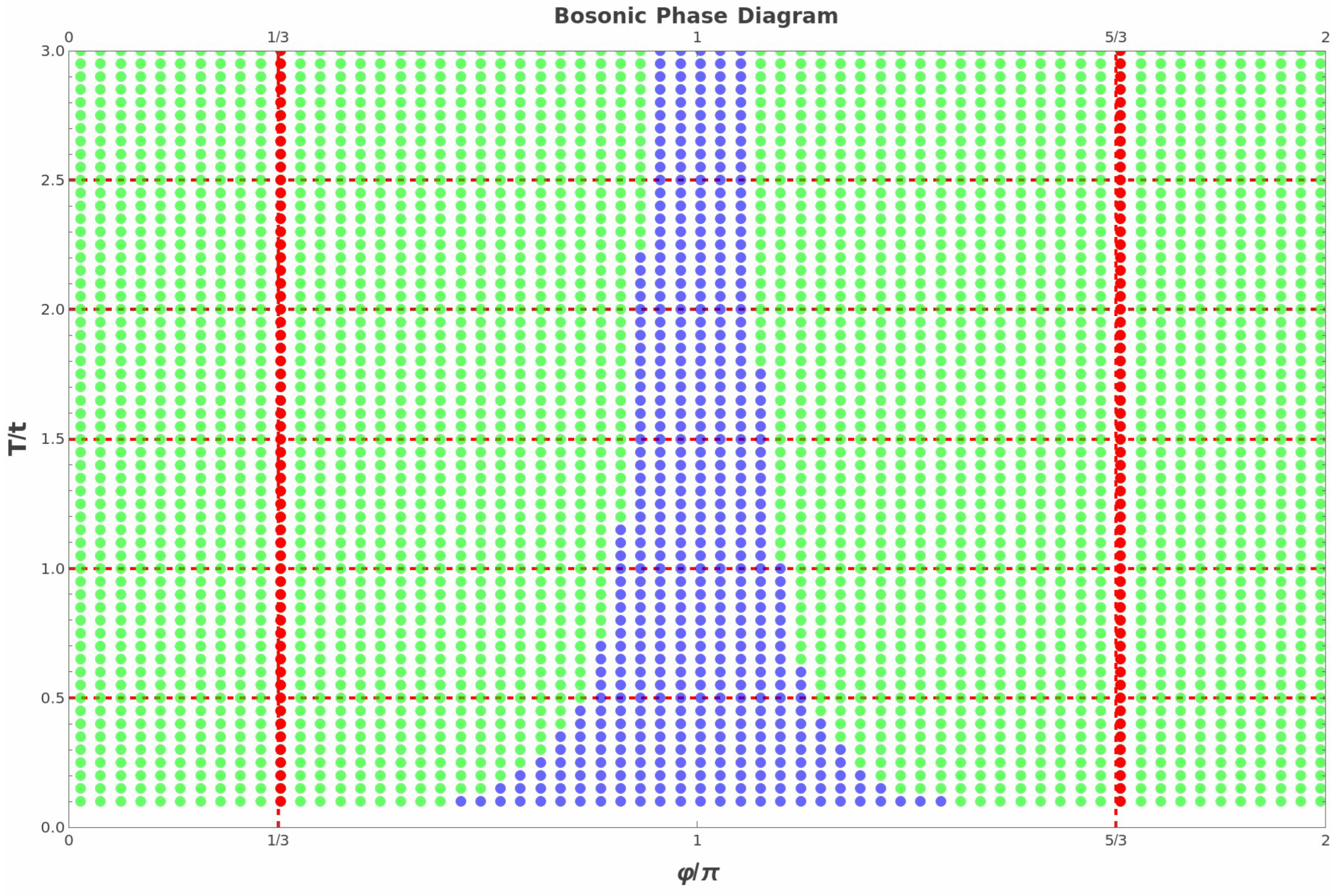
• ${\delta }_u-C_{\mathrm{UV}}<0$. This requires ${\mathcal{F}}_{\mathrm{low}}<0$, which arises when low-energy modes are suppressed relative to higher-energy contributions. This corresponds to $g(ϵ,\varphi )<1$ in the infrared, inducing an effective exclusion principle that leads to emergent fermionization, as illustrated in Figure 1.

Importantly, the mimicking of a fermionic regime does not occur just because $g<1$, but because $g(ϵ,\varphi )$ creates a competition between low energy suppression and high energy enhancement. This competition is realized inside the thermal window $\varphi \in [\pi /3,5\pi /3]$, where the kernel changes its relative weighting across energy scales. Outside that window, $g(ϵ,\varphi )>1$ for all energies, and the system reduces to a conventional bosonic regime without fermionization effects. The phase structure of the model is depicted in Figure 1. Notably, lowering $T/t$ signifies that thermal fluctuations are reduced. Inside the thermal window $\varphi \in [\pi /3,5\pi /3]$, the low-energy modes dominate the gap equation. These low-energy modes push ${\delta }_u$ to be negative, favoring $U>U_c$ (strong repulsion), which is the fermionization-like regime. In contrast, at higher temperatures, thermal excitations push ${\delta }_u$ to be positive, favoring Bose-like behavior.

Remarkably, the configuration $e^{-x}=1/2$ plays a role similar to the appearance of $ln2$ in the $C{P}^{N-1}$ model at imaginary chemical potential, as shown in Refs. [9,10]. In this case, while in the continuous model, this configuration appears as the free energy density, but, in the formulation here, it emerges through the structure of the thermal kernel.

4.3. Extrema of $N_b\left(\varphi \right)$ at $\varphi =\pi /3,5\pi /3$

The extrema and curvature of the boson number $N_b\left(\varphi \right)$ are analyzed for the repulsive Bose–Hubbard model at imaginary chemical potential. Using the Bose distribution identity

$$f_B(E-i\varphi )-f_B(E+i\varphi )={\displaystyle \frac{sin\varphi }{cosh\left(\beta E\right)-cos\varphi }},$$

(47)

the boson number at $\mathrm{\Phi }=0$ reads

$$N_b(\varphi ,T)={\int }_{-2t}^{2t}dϵ\rho \left(ϵ\right){\displaystyle \frac{sin\varphi }{cosh\left(\beta \right|ϵ\left|\right)-cos\varphi }}.$$

(48)

Assuming band symmetry

$$\rho \left(ϵ\right)=\rho (-ϵ),$$

(49)

the integrand is an even function of $ϵ$. If the functions

$$I_B\left(\varphi \right)={\int }_{-2t}^{2t}dϵ\rho \left(ϵ\right){\displaystyle \frac{1}{cosh\left(\beta \right|ϵ\left|\right)-cos\varphi }},$$

(50)

and

$$J_B\left(\varphi \right)={\int }_{-2t}^{2t}dϵ\rho \left(ϵ\right){\displaystyle \frac{1}{{\left(cosh\left(\beta \right|ϵ\left|\right)-cos\varphi \right)}^2}}$$

(51)

are defined, then the first derivative is

$${\displaystyle \frac{d{N}_b}{d\varphi }}=cos\varphi I_B\left(\varphi \right)-{sin}^2\varphi J_B\left(\varphi \right).$$

(52)

Stationary points are determined by

$$cos\varphi I_B\left(\varphi \right)-{sin}^2\varphi J_B\left(\varphi \right)=0.$$

(53)

At the particular angles $\varphi =\pi /3$ and $5\pi /3$, the parameters evaluate to $cos\varphi =1/2$ and ${sin}^2\varphi =3/4$, so Equation (53) yields

$${\displaystyle \frac{1}{2}}{I}_B-{\displaystyle \frac{3}{4}}{J}_B=0⟹J_B={\displaystyle \frac{2}{3}}{I}_B.$$

(54)

Differentiating Equation (52) gives

$${\displaystyle \frac{d^2{N}_b}{d{\varphi }^2}}=-sin\varphi I_B-3sin\varphi cos\varphi J_B-{sin}^2\varphi J_B^{\prime },$$

(55)

by using the identity

$$I_B^{\prime }\left(\varphi \right)=-sin\varphi J_B\left(\varphi \right).$$

(56)

Using $sin\varphi =\sqrt{3}/2$ and $cos\varphi =1/2$, Equation (55) gives

$${\displaystyle \frac{d^2{N}_b}{d{\varphi }^2}}{|}_{\varphi =\pi /3}=-{\displaystyle \frac{\sqrt{3}}{2}}{I}_B-{\displaystyle \frac{3\sqrt{3}}{4}}{J}_B-{\displaystyle \frac{3}{4}}{J}_B^{\prime }.$$

(57)

From Equation (54), one obtains

$${\displaystyle \frac{d^2{N}_b}{d{\varphi }^2}}{|}_{\varphi =\pi /3}=-\sqrt{3}{I}_B-{\displaystyle \frac{3}{4}}{J}_B^{\prime }.$$

(58)

The derivative $J_B^{\prime }\left(\varphi \right)$ is given by

$$J_B^{\prime }\left(\varphi \right)=-2sin\varphi {\int }_{-2t}^{2t}dϵ\rho \left(ϵ\right){\displaystyle \frac{1}{{\left(cosh\left(\beta \right|ϵ\left|\right)-cos\varphi \right)}^3}}.$$

(59)

At $\varphi =\pi /3$, $sin\varphi >0$ and then the integrand is positive, so

$$J_B^{\prime }(\pi /3)<0$$

(60)

and, as soon as $I_B>0$, the curvature is determined by a competition between the regular contribution $I_B$ and the more infrared-sensitive term $J_B^{\prime }$.

At $\varphi =5\pi /3$, one takes $sin\varphi =-\sqrt{3}/2$ and $cos\varphi =1/2$, leading to

$${\displaystyle \frac{d^2{N}_b}{d{\varphi }^2}}{|}_{\varphi =5\pi /3}=\sqrt{3}{I}_B-{\displaystyle \frac{3}{4}}{J}_B^{\prime }.$$

(61)

In this case, as soon as $sin\varphi <0$, one finds

$$J_B^{\prime }(5\pi /3)>0$$

(62)

and, since $I_B>0$, the curvature is determined again by the same competition between $I_B$ and $J_B^{\prime }$. Consequently, unlike the fermionic case, where extrema arise symmetrically from the phase structure, the bosonic extrema exhibit an intrinsic dynamical competition originating from the sign structure of the thermal kernel. This reflects the point that fermionic exclusion is fundamental, whereas, in the bosonic model, the phase dependence modifies the thermal weighting of low-energy states. This is due to the infrared enhancement of the bosonic kernel, which makes the curvature sensitive to low-energy modes. As a result, the angles $\varphi =\pi /3,5\pi /3$ do not correspond to fixed maxima or minima, but rather to points of maximal susceptibility where the system dynamically selects between a particle-like $d^2{N}_b/d{\varphi }^2<0$, “in the sense of a net particle excess” (local maximum ), and a hole-like $d^2{N}_b/d{\varphi }^2>0$, “in the sense of a net particle deficit” (local minimum) behavior.

5. Notes on Attractive Fermi–Hubbard Model at Large-N Formulation

Throughout this section, it is essential to recall the physics of the main results from the attractive Fermi–Hubbard model [28] with an imaginary chemical potential $\mu =i\theta$, which acts as a phase twist in imaginary time and modifies the Matsubara frequencies as $i{\omega }_n\to i{\omega }_n+i\theta$.

The inverse fermionic Green’s function in Nambu space takes the following form:

$${\mathcal{G}}^{-1}(i{\omega }_n,\mathbf{k})=\left(\begin{array}{cc}(i{\omega }_n+i\theta )-{ϵ}_{\mathbf{k}}& \mathrm{\Delta }\\ {\mathrm{\Delta }}^{*}& (i{\omega }_n+i\theta )+{ϵ}_{\mathbf{k}}\end{array}\right)$$

(63)

(with $\mathrm{\Delta }$ the order parameter), abberviations etc. in each of the main parts of te hpaper. Please consider. which preserves particle–hole symmetry. The quasiparticle spectrum is determined by

$$E_{\mathbf{k}}=\sqrt{{ϵ}_{\mathbf{k}}^2+{\left|\mathrm{\Delta }\right|}^2},$$

(64)

and the determinant of the Green’s function is

$$det{\mathcal{G}}^{-1}={(i{\omega }_n+i\theta )}^2-E_{\mathbf{k}}^2.$$

(65)

The thermodynamic potential is given by

$$\mathrm{\Omega }={\displaystyle \frac{{\left|\mathrm{\Delta }\right|}^2}{2U}}-\int {\displaystyle \frac{dk}{2\pi }}{E}_k-{\displaystyle \frac{1}{\beta }}\int {\displaystyle \frac{dk}{2\pi }}ln\left[1+2e^{-\beta E_k}cos\varphi +e^{-2\beta E_k}\right],$$

(66)

with $\varphi =\beta \theta$. The gap equation then becomes

$${\displaystyle \frac{1}{U}}=\int {\displaystyle \frac{dk}{2\pi }}{\displaystyle \frac{1}{E_k}}\left[1-f(E_k+i\theta )-f(E_k-i\theta )\right],$$

(67)

where $f\left(x\right)=1/(e^{\beta x}+1)$ is the Fermi–Dirac distribution. The fermion number equation reads

$$N_f=\int {\displaystyle \frac{dk}{2\pi }}\left[f(E_k-i\theta )-f(E_k+i\theta )\right],$$

(68)

which measures the imbalance between particle-like and hole-like excitations induced by the imaginary chemical potential. The thermodynamics is governed by the fermionic thermal kernel

$$g_F(x,\varphi )={\displaystyle \frac{sinhx}{coshx+cos\varphi }},x=\beta E_k.$$

(69)

The kernel (69) satisfies

$$g_F(x,\varphi )-1={\displaystyle \frac{cos\varphi -e^{-x}}{coshx+cos\varphi }},$$

(70)

which determines the sign structure of contributions to the gap equation. The specific angles $\varphi =2\pi /3$ and $\varphi =4\pi /3$ (where $cos\varphi =-1/2$) define a universal thermal window $\varphi \in [\pi /3,5\pi /3]$ where the kernel changes sign at $x_{*}=ln2$.

Inside this thermal window, spectral weight is redistributed between low-energy and high-energy modes, leading to enhanced pairing correlations and driving the BCS–BEC crossover. The crossover is controlled by the parameter

$${\delta }_u={\displaystyle \frac{1}{U}}-{\displaystyle \frac{1}{U_c}},$$

(71)

where ${\delta }_u<0$ corresponds to the BEC regime (strong attraction) and ${\delta }_u>0$ to the BCS regime (weak attraction). The imaginary chemical potential acts as a statistical regulator, continuously tuning the system between different pairing regimes by modifying the entropy contribution to the free energy. At the critical point ${\delta }_u=0$, the system exhibits universal behavior characterized by a thermal window which plays a central role in determining the phase structure.

6. Mapping Between Attractive Fermi and Repulsive Bose–Hubbard Models at Imaginary Chemical Potential

6.1. Formal Mapping via Matsubara Frequencies

The partition function for fermions with imaginary chemical potential $i\theta$ is given by

$${\mathcal{Z}}_F\left(\theta \right)=\prod _{\mathbf{k},n}\left[{(i{\omega }_n^F+i\theta )}^2-E_{\mathbf{k}}^2\right],{\omega }_n^F={\displaystyle \frac{(2n+1)\pi }{\beta }}.$$

(72)

For bosons, the Matsubara frequencies are ${\omega }_n^B=2n\pi /\beta$. Using the relation ${\omega }_n^B={\omega }_n^F+\pi /\beta$, one obtains

$$i{\omega }_n^B+i\theta =i{\omega }_n^F+i(\theta +\pi ).$$

(73)

Consequently,

$${\mathcal{Z}}_B\left(\theta \right)·{\mathcal{Z}}_F(\theta +\pi )=1$$

(74)

since, at the level of the unconstrained functional integrals, bosonic Gaussian integration fields yield inverse determinants while fermionic fields yield determinants. Thus, within the large-N saddle point framework, the thermodynamic behavior and the single-particle thermal kernels of the repulsive Bose–Hubbard model at imaginary chemical potential $\theta$ are mapped via a formal analytic continuation to the attractive Fermi–Hubbard model at $\theta +\pi$. Within the fermionization-like window, the free energy $F=U-TS$, where S is the entropy, is minimized by interaction avoidance since the phase twist increases effective density pressure. Then, bosons are rearranged into higher energy levels, mimicking Pauli exclusion to avoid the repulsive interaction cost U. Also, entropic gain causes the fermionized distribution to occupy a larger spectral range than a standard Bose–Einstein condensate, lowering F.

6.2. Mapping Between Fermionic and Bosonic Thermal Kernels

The fermionic thermal kernel derived from the attractive Hubbard model is

$$g_F(x,\varphi )={\displaystyle \frac{sinhx}{coshx+cos\varphi }},x=\beta E_k,\varphi =\beta \theta .$$

(75)

For the repulsive Bose–Hubbard model, the corresponding bosonic thermal kernel is

$$g_B(x,\varphi )={\displaystyle \frac{sinhx}{coshx-cos\varphi }}.$$

(76)

The two kernels are related by a plain shift of the imaginary chemical potential:

$$g_B(x,\varphi )=g_F(x,\varphi +\pi ).$$

(77)

Indeed, using $cos(\varphi +\pi )=-cos\varphi$, one obtains

$$g_F(x,\varphi +\pi )={\displaystyle \frac{sinhx}{coshx+cos(\varphi +\pi )}}={\displaystyle \frac{sinhx}{coshx-cos\varphi }}=g_B(x,\varphi ).$$

(78)

This mapping reflects the underlying thermodynamic duality between the attractive Fermi and repulsive Bose–Hubbard models at imaginary chemical potential and at the level of the single-particle thermal kernels, with the shift $\varphi \to \varphi +\pi$ exchanging the roles of the two statistics in the saddle point free energy.

7. Universal Statistical Transmutation Framework at Imaginary Chemical Potential

A generic interacting lattice system is considered at finite temperature with an imaginary chemical potential $\mu =i\theta$. The grand-canonical partition function can be written in the following form:

$$\mathcal{Z}\left(\varphi \right)=\prod _{\mathbf{k},n}{\left[{(i{\omega }_n+i\theta )}^2-E_{\mathbf{k}}^2\right]}^{\sigma },$$

(79)

where $\sigma =+1$ for fermions and $\sigma =-1$ for bosons. Taking the logarithm and performing the Matsubara sum yields the universal free energy density

$${\mathrm{\Omega }}_{\sigma }\left(\varphi \right)={\displaystyle \frac{\sigma {\gamma }_{\sigma }^2}{2U}}-\int {\displaystyle \frac{d^{d}k}{{\left(2\pi \right)}^d}}\left[\sigma E_{\mathbf{k}}+{\displaystyle \frac{\sigma }{\beta }}ln\left(1+\sigma 2e^{-\beta E_{\mathbf{k}}}cos\varphi +e^{-2\beta E_{\mathbf{k}}}\right)\right].$$

(80)

where ${\gamma }_{+1}\equiv \mathrm{\Delta }$ and ${\gamma }_{-1}\equiv \mathrm{\Phi }$, and this expression unifies fermionic and bosonic statistics through the parameter $\sigma$. Differentiating the free energy with respect to E yields the universal occupation kernel

$$g_{\sigma }(x,\varphi )={\displaystyle \frac{sinhx}{coshx+\sigma cos\varphi }},x=\beta E.$$

(81)

The kernel (81) governs all thermodynamic observables for:

• fermions ($\sigma =+1$),

  $$g_F(x,\varphi )={\displaystyle \frac{sinhx}{coshx+cos\varphi }};$$

  (82)
• bosons ($\sigma =-1$),

  $$g_B(x,\varphi )={\displaystyle \frac{sinhx}{coshx-cos\varphi }}.$$

  (83)

Therefore, the free energy densities obey

$${\mathrm{\Omega }}_B\left(\varphi \right)=-{\mathrm{\Omega }}_F(\varphi +\pi ).$$

(84)

This establishes a precise duality:

Bosonic thermal kernel at phase $\varphi$ is equivalent to fermionic thermal kernel at phase $\varphi +\pi$.

The kernel (81) satisfies the following:

$$g_{\sigma }(x,\varphi )-1={\displaystyle \frac{cos\varphi -e^{-x}}{coshx+\sigma cos\varphi }}.$$

(85)

The sign change occurs at

$$e^{-x_{*}}=cos\varphi .$$

(86)

Thus for:

• fermions ($\sigma =+1$), critical angle $\varphi =2\pi /3$;
• bosons ($\sigma =-1$), critical angle $\varphi =\pi /3$.

This reveals a universal ${\mathbb{Z}}_3$ structure:

$${\varphi }_c^{\left(B\right)}={\varphi }_c^{\left(F\right)}+\pi .$$

(87)

The order parameter $\mathrm{\Delta }$ (fermions) or $\mathrm{\Phi }$ (bosons) satisfies the unified equation:

$${\displaystyle \frac{1}{U}}-{\displaystyle \frac{1}{U_c}}=\int dϵ\rho \left(ϵ\right)\left[{\displaystyle \frac{g_{\sigma }(\beta E,\varphi )}{E}}-{\displaystyle \frac{1}{ϵ}}\right].$$

(88)

The single Equation (88) describes the BCS–BEC crossover for fermions, the fermionization-like crossover for bosons, and dimensional effects via $\rho \left(ϵ\right)$. It is noteworthy that, after this map between the two theories, it can be stated that the imaginary chemical potential shifts Matsubara frequencies, modifies occupation statistics, and creates effective exclusion. The free energy then becomes

$$F=U-TS\left(\varphi \right),$$

(89)

where $\varphi$ controls the entropy functional.

On the other hand, if one aims to find the critical thermal window at unitarity then using the Landau theory of phase transitions by expanding the thermal potential near a critical point, the phase boundary is determined by

$$a_2(T,\varphi )=0$$

(90)

with

$$a_2={\delta }_u-\int dϵ\rho \left(ϵ\right){\displaystyle \frac{g_{\sigma }(\beta ϵ,\varphi )-1}{ϵ}},$$

(91)

resulting from the analytical calculation in Appendix A. In

Table 1. Mapping between attractive fermions and repulsive bosons at imaginary chemical potential. See text for details.

Feature	Fermions (Attractive)	Bosons (Repulsive)
Interaction	$-\left|U\right|$ (attractive)	$+U$ (repulsive)
Thermal window	$2\pi /3<\varphi <4\pi /3$	$\pi /3<\varphi <5\pi /3$
Inside behavior	BCS/BEC possible	Fermi-like behavior possible
Low temperature ($T/t<1$)
Inside thermal window	BEC-like (more pairing)	Fermi-like (more spreading)
Outside thermal window	Normal fermions	Pure bosons
High temperature ($T/t>1$)
Inside thermal window	Pairing fluctuations suppressed	Bose-like (less spreading)
Outside thermal window	Normal fermions	Standard Bose-enhanced regime
Coupling strength (${\delta }_u=1/U-1/U_c$)
${\delta }_u<0$ ($U>U_c$)	More pairing (BEC)	More spreading (Fermi-like)
${\delta }_u>0$ ($U<U_c$)	Less pairing (BCS)	Less spreading (Bose-like)
${\delta }_u=0$	Unitarity (critical)	Fermi-like behavior point (critical)

, the mapping picture where the BCS–BEC crossover and bosonic phase-induced fermion-like behavior arise from the same underlying mechanism is shown.

8. Discussion

A formal thermodynamic mapping has been established between the attractive Fermi–Hubbard model and the repulsive Bose–Hubbard model at the level of thermal kernels at finite temperature in the presence of an imaginary chemical potential $\mu =i\theta$. Using the relation ${\omega }_n^B={\omega }_n^F+\pi /\beta$ between bosonic and fermionic Matsubara frequencies, one can find ${\mathcal{Z}}_B\left(\theta \right)·{\mathcal{Z}}_F(\theta +\pi )=1$, which maps the repulsive Bose–Hubbard model onto the attractive Fermi–Hubbard model shifted by $\pi$. Consequently, the thermal kernels satisfy $g_B(x,\varphi )=g_F(x,\varphi +\pi )$ with $\varphi =\beta \theta$, and the unified kernel $g_{\sigma }(x,\varphi )=sinhx/(coshx+\sigma cos\varphi )$ (with $\sigma =+1$ for fermions and $\sigma =-1$ for bosons) governs both models. The condition $g_{\sigma }(x,\varphi )=1$ yields $x_{*}=ln2$ when $cos\varphi =-\sigma /2$, which interestingly defines the universal thermal window boundaries: $\varphi =2\pi /3,4\pi /3$ for fermions and $\varphi =\pi /3,5\pi /3$ for bosons. Inside these windows, spectral weight is redistributed between lower- and higher-energy modes.

For fermions inside the thermal window, ${\delta }_u=1/U-1/U_c<0$ (strong attraction) favors BEC-like pairing, while ${\delta }_u>0$ (weak attraction) favors BCS-like behavior. For bosons inside the thermodynamic fermionization crossover window, ${\delta }_u<0$ (strong repulsion) favors Fermi-like spreading while ${\delta }_u>0$ (weak repulsion) favors Bose-like behavior. In both cases, lowering $T/t$ enhances the specific behavior inside the window, as the entropy term $-TS$ becomes less dominant and the interaction energy governs the free energy $F=U-TS$. The imaginary chemical potential thus acts as a temporal gauge field that continuously interpolates between Bose and Fermi statistics, with dimensionality entering only through the density of states $\rho \left(ϵ\right)$.

The results obtained here provides a novel view into the physics of emergent fermionization and Bose–Fermi mapping at finite temperature since this mapping unifies BCS-BEC crossover in fermions and Fermi-statistical emulation in bosons within a single framework. In contrast to the fermionic case, where the extrema of the fermion number $N_f\left(\varphi \right)$ are rigidly fixed by particle–hole symmetry, the extrema of the boson number $N_b\left(\varphi \right)$ lack such universal symmetry constraints. Consequently, the bosonic curvature exhibits a dynamic selection of particle- or hole-like behavior at the thermal window boundaries, where the system characteristically locks into fixed maxima or minima, respectively.

Although boson–fermion mappings at imaginary chemical potential have been explored in field-theoretic contexts [9,10], the interplay between imaginary chemical potential and fermionization in lattice bosonic and fermionic systems remains largely unexplored. The present findings imply that they may be extended in several new directions and present remarkable progress in the understanding of duality identities, like an overall Fermi–Boson–Hubbard model coupled to a gauge field, and it will be of high interest to examine the theory developed here with experimental results arising from the appearance of synthetic gauge fields or Floquet engineering techniques [29]. This may be an opened capability to ultracold atoms like those considered in Ref. [30], where the anyon statistical angle is the closest experimental analog to $\varphi$ from imaginary chemical potential here. Also, a Bose–Fermi–Hubbard map for general d dimensions believed to be an attarctive concept, along with the Fermi-like windows, as a generalization to the one-dimensional results or to examine if the edges of thermal windows are at different angles determined by the zeros or extrema of Clausen functions. Finally, a possible generalization of this study to disorder Hubbard models, such as that in Ref. [31], is believed to give quite interesting results.

References

1. Zwerger, W. (Ed.) The BCS–BEC Crossover and the Unitary Fermi Gas; Springer: Berlin/Heidelberg, Germany, 2012. [Google Scholar] [CrossRef]
2. Garg, A.; Krishnamurthy, H.R.; Randeria, M. BCS–BEC crossover at T = 0: A dynamical mean-field theory approach. Phys. Rev. B 2005, 72, 024517. [Google Scholar]
3. Diener, R.B.; Sensarma, R.; Randeria, M. Quantum fluctuations in the superfluid state of the BCS–BEC crossover. Phys. Rev. A 2008, 77, 023626. [Google Scholar]
4. Bauer, J.; Hewson, A.C.; Dupuis, N. Dynamical mean-field theory and numerical renormalization group study of superconductivity in the attractive Hubbard model. Phys. Rev. B 2009, 79, 214518. [Google Scholar] [CrossRef][Green Version]
5. Capogrosso-Sansone, B.; Prokof’ev, N.V.; Svistunov, B.V. Phase diagram and thermodynamics of the three-dimensional Bose–Hubbard model. Phys. Rev. B 2007, 75, 134302. [Google Scholar]
6. Kagan, M.Y.; Bianconi, A. Fermi–Bose mixtures and BCS–BEC crossover in high-Tc superconductors. Condens. Matter 2019, 4, 51. [Google Scholar]
7. Dell’Anna, L.; De Bettin, F.; Salasnich, L. Rabi coupled fermions in the BCS–BEC crossover. Condens. Matter 2022, 7, 59. [Google Scholar] [CrossRef]
8. Fujita, M.; Meyer, R.; Pujari, S.; Tezuka, M. Effective hopping in holographic Bose and Fermi–Hubbard models. J. High Energ. Phys. 2019, 2019, 45. [Google Scholar]
9. Filothodoros, E.G.; Petkou, A.C.; Vlachos, N.D. 3d fermion–boson map with imaginary chemical potential. Phys. Rev. D 2017, 95, 065029. [Google Scholar]
10. Filothodoros, E.G.; Petkou, A.C.; Vlachos, N.D. The fermion–boson map for large d. Nucl. Phys. B 2019, 941, 195–224. [Google Scholar] [CrossRef]
11. Bonkhoff, M.; Jäger, S.B.; Schneider, I.; Pelster, A.; Eggert, S. Coherence properties of the repulsive anyon–Hubbard dimer. Phys. Rev. B 2023, 108, 155134. [Google Scholar]
12. Pupillo, G.; Rey, A.M.; Williams, C.J.; Clark, C.W. Extended fermionization of 1D bosons in optical lattices. New J. Phys. 2006, 8, 161. [Google Scholar] [CrossRef]
13. Alford, M.; Kapustin, A.; Wilczek, F. Imaginary chemical potential and finite fermion density on the lattice. Phys. Rev. D 1999, 59, 054502. [Google Scholar] [CrossRef]
14. Girardeau, M. Relationship between systems of impenetrable bosons and fermions in one dimension. J. Math. Phys. 1960, 1, 516–523. [Google Scholar] [CrossRef]
15. Paredes, B.; Widera, A.; Murg, V.; Mandel, O.; Fölling, S.; Cirac, I.; Shlyapnikov, G.V.; Hänsch, T.W.; Bloch, I. Tonks–-Girardeau gas of ultracold atoms in an optical lattice. Nature 2004, 429, 277–281. [Google Scholar] [PubMed]
16. Bera, S.; Chakrabarti, B.; Gammal, A.; Tsatsos, M.C.; Lekala, M.L.; Chatterjee, B.; Lévêque, C.; Lode, A.U. Sorting fermionization from crystallization in many-boson wavefunctions. Sci. Rep. 2019, 9, 17873. [Google Scholar] [CrossRef] [PubMed]
17. Muraev, P.S.; Maksimov, D.N.; Kolovsky, A.R. Signatures of quantum chaos and fermionization in the incoherent transport of bosonic carriers in the Bose–Hubbard chain. Phys. Rev. E 2024, 109, L032107. [Google Scholar] [PubMed]
18. Maiti, S.; Sedrakyan, T. Fermionization of bosons in a flat band. Phys. Rev. B 2019, 99, 174418. [Google Scholar] [CrossRef]
19. Lelas, K.; Ševa, T.; Buljan, H.; Goold, J. Pinning quantum phase transition in a Tonks–Girardeau gas: Diagnostics by ground-state fidelity and the Loschmidt echo. Phys. Rev. A 2012, 86, 033620. [Google Scholar]
20. Boesl, J.; Dilip, R.; Pollmann, F.; Knap, M. Characterizing fractional topological phases of lattice bosons near the first Mott lobe. Phys. Rev. B 2022, 105, 075135. [Google Scholar] [CrossRef]
21. Iskin, M. Artificial gauge fields for the Bose–Hubbard model on a checkerboard superlattice and extended Bose–Hubbard model. Eur. Phys. J. B 2012, 85, 76. [Google Scholar]
22. Carr, L.D.; Holland, M.J. Quantum phase transitions in the Fermi–Bose Hubbard model. Phys. Rev. A 2005, 72, 031604. [Google Scholar] [CrossRef][Green Version]
23. Cazalilla, M.A.; Citro, R.; Giamarchi, T.; Orignac, E.; Rigol, M. One dimensional bosons: From condensed matter systems to ultracold gases. Rev. Mod. Phys. 2011, 83, 1405–1466. [Google Scholar] [CrossRef]
24. Vitoriano, C.; Nancy, K.; Rocha, S.; Coutinho-Filho, M.D. Hubbard model with infinite-range attractive interaction. Phys. Rev. B 2005, 72, 165109. [Google Scholar] [CrossRef]
25. Giering, K.-U.; Salmhofer, M. Self-energy flows in the two-dimensional repulsive Hubbard model. Phys. Rev. B 2012, 86, 245122. [Google Scholar]
26. Roberge, A.; Weiss, N. Gauge theories with imaginary chemical potential and the phases of QCD. Nucl. Phys. B 1986, 275, 734–745. [Google Scholar] [CrossRef]
27. Žitko, R.; Osolin, Ž.; Jeglič, P. Repulsive versus attractive Hubbard model: Transport properties and spin-lattice relaxation rate. Phys. Rev. B 2015, 91, 155111. [Google Scholar] [CrossRef]
28. Filothodoros, E.G. Thermal phase structure of the attractive Fermi Hubbard model with imaginary chemical potential. arXiv 2026, arXiv:2604.18798. [Google Scholar] [CrossRef]
29. Lienhard, V.; Scholl, P.; Weber, S.; Barredo, D.; de Léséleuc, S.; Bai, R.; Lang, N.; Fleischhauer, M.; Büchler, H.P.; Lahaye, T.; et al. Realization of a density-dependent Peierls phase in a synthetic, spin–orbit coupled Rydberg system. Phys. Rev. X 2020, 10, 021031. [Google Scholar]
30. Bonkhoff, M.; Jägering, K.; Eggert, S.; Pelster, A.; Thorwart, M.; Posske, T. Bosonic continuum theory of one-dimensional lattice anyons. Phys. Rev. Lett. 2021, 126, 163201. [Google Scholar] [CrossRef] [PubMed]
31. Prasad, Y.; Lee, H. Interplay of disorder and interactions in the bilayer band insulator: A determinant quantum Monte Carlo study. Phys. Rev. B 2024, 109, 064506. [Google Scholar] [CrossRef]
Figure 1. Bose–Fermi crossover for F + C UV for the Bose–Hubbard model at imaginary chemical potential and δ u = 0 . Lower T / t signifies that entropy term T S becomes less negative and so U term dominates. Then, the system spreads out to avoid repulsion producing a more fermion-like occupation. The blue region indicates the regime dominated by low-energy mode suppression ( g B < 1 ), green corresponds to conventional bosonic enhancement ( g B > 1 ), and red dots at β θ = π / 3 , 5 π / 3 mark where Φ = 0 and N b is maximized. The parameters used are t = 1 , Λ = 0.5 , C UV = + 5.2 . The magnitude and sign of the “ultraviolet” constant C UV are determined by the high-energy behavior of the dispersion relation. For fermions, the low-energy dispersion is linear, ϵ k k , leading to a logarithmic divergence in the integral d k / k . For bosons, the dispersion is quadratic, ϵ k k 2 , which produces a much stronger linear divergence d k / k 2 . As a result, the raw integral inside the fermionization window is highly negative. To overcome this large negative contribution and reveal a well-balanced and visible blue ( g B < 1 ) Fermi-like region compared to the green area, a representative choice C U V = + 5.2 is used, in order to achieve a negative (enhanced fermionization regime) δ u eff . If a smaller C UV is chosen, then the green (Bose-like) area dominates. See text for details.
Physics 08 00054 g001