Use of Redshifts as Evidence of Dark Energy

Abstract

The large-scale dynamics of the universe is generally described in terms of the time-dependent scale factor $a\left(t\right)$. To make contact with observational data, the $a\left(t\right)$ function needs to be related to the observable $z\left(r\right)$ function, redshift versus distance. Model fitting of data has shown that the equation that governs $z\left(r\right)$ needs to contain a constant term, which has been identified as Einstein’s cosmological constant. Here, it is shown that the required constant term is not a cosmological constant but is due to an overlooked geometric difference between proper time t and look-back time $t_{\mathrm{lb}}$ along lines of sight, which fan out isotropically in all directions of the 3D (3-dimensional) space that constitutes the observable universe. The constant term is needed to satisfy the requirement of spatial isotropy in the local limit. Its magnitude is independent of the epoch in which the observer lives and agrees with the value found by model fitting of observational data. Two of the observational consequences of this explanation are examined: an increase in the age of the universe from 13.8 Gyr to 15.4 Gyr, and a resolution of the $H_0$ tension, which restores consistency to cosmological theory.

1. Introduction

The physical nature of the cosmological constant $\Lambda$ that was introduced by Albert Einstein [1] (see English translation in Ref. [2]) a century ago has remained an enigma. It was unexpectedly found necessary to reintroduce $\Lambda$ in 1998 as a fitting parameter to allow for modeling of redshift z versus distance r in terms of the FLRW (Friedmann–Lemaître–Robertson–Walker) framework for observations of supernovae type Ia as standard candles [3,4]. If the $\Lambda$ term is placed on the right-hand side of the Einstein field equation and considered as a physical field that is a component ${\rho }_{\Lambda }$ (commonly referred to as “dark energy”) of the energy-momentum tensor, then the observed sign and magnitude of this field represents a repulsive gravity force that permeates all of space without any significant spatial structuring, driving an accelerated cosmic expansion; see [5,6,7,8,9,10]. Furthermore, as the magnitude of ${\rho }_{\Lambda }$ is found to be of the same order as the matter density ${\rho }_M$, although ${\rho }_M$ varies with redshift as ${(1+z)}^3$ while ${\rho }_{\Lambda }$ is independent of z, the present epoch seems to be singled out as special. Such a “cosmic coincidence” violates the Copernican principle, which states that we are not privileged observers.

While the supernovae observations that were reported in 1998 represented the remarkable discovery of an unexpected property of the redshift–distance relation $z\left(r\right)$, the interpretation of the redshift data in terms of an accelerated cosmic expansion as driven by some “dark energy” depends on a theoretical model for the relation between the observable $z\left(r\right)$ function and the $a\left(t\right)$ function that describes the dynamics and evolution of the universe in terms of scale factor a versus time t. As the time dependence of the scale factor is not directly observable, it is inferred from a static historical record of a sequence of past discrete events like in archaeology. In the case of cosmology, the static timeline of past historical events is accessed by looking out in space. Due to the finite speed of light, distance from the observer and look-back time are equivalent coordinates. When cosmic distances are measured with the help of the astrophysical “distance ladder”—which makes use of “standard candles”—in particular supernovae, the corresponding look-back times are also obtained.

This “cosmic archeology” can allow us to infer the dynamical properties of the universe, but only if it is known how to relate the observable, “archeological” $z\left(r\right)$ function to the dynamic, non-observable $a\left(t\right)$ function. In the past, the conversion from $a\left(t\right)$ to $z\left(r\right)$ has been taken care of in a straightforward way: in the FLRW equation that governs the $a\left(t\right)$ function, one replaces a with z via the relation $a=1/(1+z)$ and identifies the expansion rate $\dot{a}/a$ with the Hubble constant $H\equiv \mathrm{d}z/\mathrm{d}r$, where the dot denotes the time derivative. The variation $a\left(t_{\mathrm{lb}}\right)$ with distance r or look-back time $t_{\mathrm{lb}}$ is obtained from the FLRW solution for the $a\left(t\right)$ function.

This procedure of standard cosmology has not been seen as a contentious issue. However, it overlooks a fundamental difference between dynamic, proper time t and look-back time $t_{\mathrm{lb}}$. The function $a\left(t_{\mathrm{lb}}\right)$ is isotropic with spherical symmetry in a static 3D (3-dimensional) space, the observable universe. The symmetry is broken when a redshift is determined, because the observation implies the selection of the particular line of sight that connects the observer with the observed object. In the local limit, however, the requirement of spatial isotropy must always be satisfied.

It is shown in the present paper that when this isotropy requirement is accounted for, the equation that governs the $z\left(r\right)$ relation acquires an additional constant term ${\Omega }_X=2/3$, which formally appears in the same way as a cosmological constant ${\Omega }_{\Lambda }$ in standard cosmology. ${\Omega }_X$ is not, however, a cosmological constant, because it does not appear in the FLRW equation that governs the $a\left(t\right)$ function. Its 2/3 value does not depend on the epoch of the observer. There is no “cosmic coincidence” problem. Other implications of the theory include an increase of the age of the universe from 13.8 Gyr to 15.4 Gyr and a resolution of the $H_0$ tension.

2. Relation Between Redshift, Time, and Distance

The formal relation between redshift z and scale factor a is seemingly simple,

$$1+z=a_0/a$$

(1)

(with normalization factor $a_0$), but the relation (1) may be a source of confused and incorrect interpretations if one is not clear enough about the coordinate frames that are used.

An example of an incorrect interpretation is when one considers the time dependence of this expression. According to a basic FLRW assumption, the scale factor is a function of time t in co-moving frames, but it does not vary with space in 3D hyperplanes that are orthogonal to the time axis. The normalization parameter $a_0$ is by convention set to unity at the location of the observer. From this, one may conclude that the redshift is time dependent, as given by $z\left(t\right)=-1+1/a\left(t\right)$, and therefore that $-\dot{z}\left(t_{\mathrm{obs}}\right)={(\dot{a}/a)}_{\mathrm{obs}}$, the expansion rate at the location of the observer.

It immediately becomes understandable that this conclusion is completely wrong, when recalling that the spacetime location of the observer defines the zero point of the redshift scale. Therefore, the redshift with all its temporal gradients, to infinite order, becomes zero at the location of the observer. Thus, $z_{\mathrm{obs}}={\dot{z}}_{\mathrm{obs}}={\ddot{z}}_{\mathrm{obs}}=0$ forever. ${\dot{z}}_{\mathrm{obs}}$ can never equal $-{(\dot{a}/a)}_{\mathrm{obs}}$.

The cause for this confusion is the neglect of the time dependence of $a_0\equiv a\left(t_{\mathrm{obs}}\right)$. At the location of the observer, the time dependence of the numerator and denominator of Equation (1), ${\dot{a}}_0$ and $\dot{a}$, become identical and compensate each other, such that the time dependence of z becomes zero, as required for consistency with the definition of redshifts.

The goal here is to derive the redshift–distance function $z\left(r\right)$ from the $a\left(t\right)$ function. The r dependence of z implies according to Equation (1) that

$$1+z\left(r\right)=1/a\left(r\right).$$

(2)

However, distance r is not a coordinate in spatial hyperplanes that are orthogonal to the time axis, because the scale factor does not vary within such hyperplanes. Instead, r is a coordinate along lines of sight in the 3D hypersurface of the past light cone.

Since lines of sight are geodesics of light rays, which are curved in normal spacetime representations because of the nonlinear cosmic expansion, it is convenient to use conformal time $\eta$ instead of proper time t, as defined by

$$\mathrm{d}\eta \equiv \mathrm{d}t/a.$$

(3)

The special advantage with conformal time is that the nonlinear expansion is compensated for in a way that makes light rays and lines of sight straight lines in a spacetime representation.

Look-back time $t_{\mathrm{lb}}$ is the temporal separation between the observer and the observed object (e.g., a galaxy):

$$t_{\mathrm{lb}}\equiv t_{\mathrm{obs}}-t,$$

(4)

where $t_{\mathrm{obs}}$ and t are the ages of the universe at the spacetime location of the observer and the observed object, respectively.

In terms of conformal time, look-back time ${\eta }_{\mathrm{lb}}$ becomes equivalent to coordinate distance r when using units, for which the speed of light c is unity (as used throughout the present paper). Thus,

$$r\equiv {\eta }_{\mathrm{lb}}={\eta }_0-\eta ,$$

(5)

where ${\eta }_0$ represents the present conformal age of the universe. It allows for a more explicit expression for the redshift:

$$1+z(r,{\eta }_0)={\displaystyle \frac{a\left({\eta }_0\right)}{a({\eta }_0-r)}}.$$

(6)

If the time dependence ${\eta }_0$ of the observer is accounted for, which is the case when the past light cone is treated as a 4D object, then the time derivative of z is zero at the observer ($r=0$), as required by the definition of the redshifts. However, the distance derivative $\partial z/\partial r$, which represents the original spatial definition of the Hubble constant, is non-zero, because r appears only in the denominator but not in the numerator, in contrast to the time coordinate.

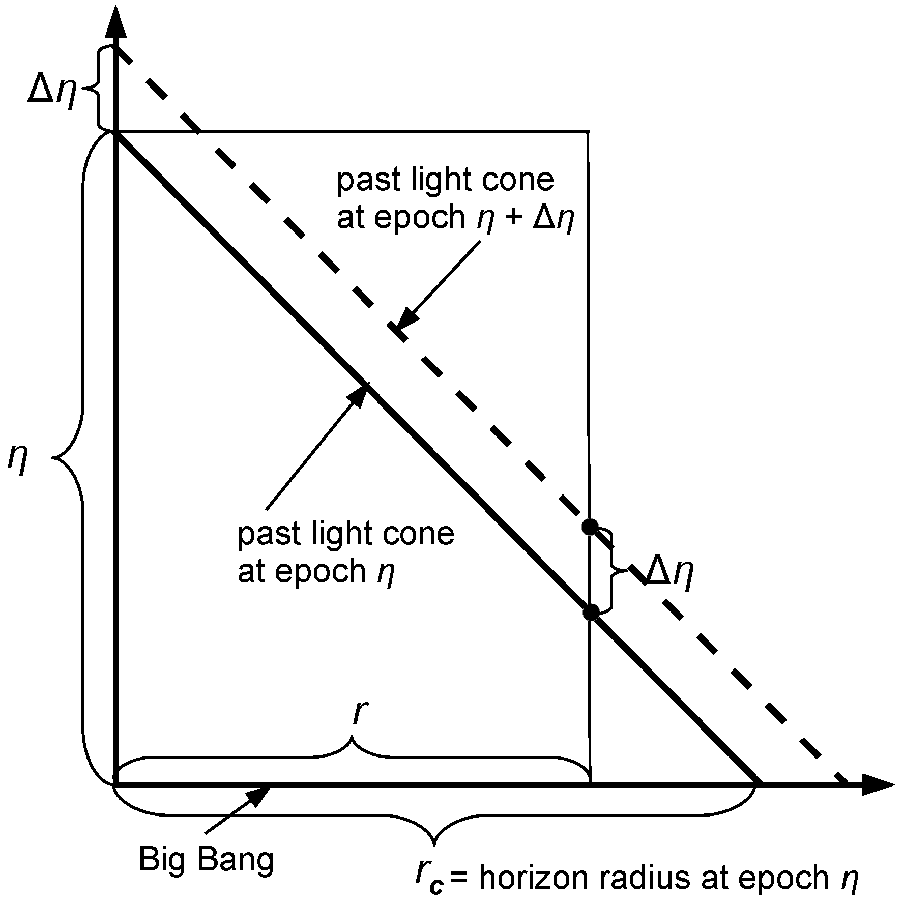
The conformal spacetime diagram of Figure 1 illustrates how the evolution of the past light cone affects the redshift observations. Redshifts z are only defined along light rays that represent lines of sight. They vary from zero at the tip of the cone, where the observer is located, to infinity at the bottom of the cone, at the Big Bang, at a distance $r_c$ (the horizon radius) from the observer.

A basic assumption of the FLRW interpretational framework is that all observed objects are co-moving, at rest with respect to the expanding spatial grid. The coordinate distances r and conformal look-back times ${\eta }_{\mathrm{lb}}$ are therefore time independent (in contrast to proper distances $ar$). It then follows from Equation (5) that $\mathrm{d}{\eta }_{\mathrm{obs}}=\mathrm{d}\eta$. Conformal time “flows” at the same rate for the observer as for the observed galaxy, independent of its distance. In contrast, proper time t flows at different rates because the scale factor varies with distance. With conformal time, the scale factor has been divided out to make the relation between distance and conformal time linear so that light rays become straight lines.

Only when one formally halts the flow of time for the observer by treating ${\eta }_0$ as a constant can one obtain a representation in which distance varies with time. Then, as follows from Equation (5), $\mathrm{d}\eta =-\mathrm{d}{\eta }_{\mathrm{lb}}=-\mathrm{d}r$. In this case, time does not “flow” but is a static coordinate along a historical record of past events. This description represents a 3D subspace, the part of 4D spacetime that is accessible to the observer at the moment of observation. It is the subspace that is referred to as the “observable universe”. As the redshift is then only a function of the single distance parameter r or ${\eta }_{\mathrm{lb}}$, the partial derivatives can be replaced by total derivatives: $\mathrm{d}z/\mathrm{d}r$ or $\mathrm{d}z/\mathrm{d}{\eta }_{\mathrm{lb}}$.

3. Geometric Aspects of Look-Back Time, Spatial Isotropy, and  Implications for $\mathit{z}\left(\mathit{r}\right)$

When making the connection between the dynamic $a\left(t\right)$ function that represents 4D spacetime and the $z\left(r\right)$ and $a\left(r\right)$ functions that represent the static 3D observable universe, different geometric aspects enter in a profound way. At first glance, $a\left(r\right)=a\left({\eta }_{\mathrm{lb}}\right)$ according to Equation (5) may seem to imply that one can simply use the $a\left(\eta \right)$ solution for $a\left(r\right)$ that follows from the dynamic $a\left(t\right)$ function, and this then immediately solves the problem. While this is what standard cosmology does, it overlooks the geometric issues that become relevant when connecting a 1D function to a function that is isotropic in a 3D vector space.

While t and $\eta$ are 1D coordinates, look-back time $t_{\mathrm{lb}}$ or ${\eta }_{\mathrm{lb}}$ are radial coordinates that run along the lines of sight that fan out in 3D space from the central point, the location of the observer, where r and $t_{\mathrm{lb}}$ are zero. Although the $a\left({\eta }_{\mathrm{lb}}\right)$ function is identical to the 1D $a\left(\eta \right)$ function along each 1D line of sight, there are infinite viewing directions. As each line of sight needs to be defined by three mutually independent parameters, there are three spatial degrees of freedom.

$a\left(r\right)$ is an isotropic function in the 3D space that defines the observable universe. The act of observation is, however, not isotropic. The observation of a given galaxy singles out a certain viewing direction, which breaks the spatial symmetry. While different galaxies correspond to different viewing directions, each single redshift measurement breaks the isotropy.

After these introductory remarks, let us see how these concepts play out for the explicit derivation of the Hubble constant and the expression for the $z\left(r\right)$ function. The starting point is the FLRW equation for the $a\left(t\right)$ function with the assumption of spatial flatness and no cosmological constant:

$${\left({\displaystyle \frac{\dot{a}}{a}}\right)}^2={\displaystyle \frac{8\pi G}{3}}\left[{\rho }_{M_0}{(a_0/a)}^3+{\rho }_{R_0}{(a_0/a)}^4\right],$$

(7)

where subscript 0 refers to the location of the observer, and G is the gravitational constant.

The squared expansion rate that describes the evolution of the universe has its sources in the mass–energy densities ${\rho }_{M,R}$ of matter and radiation. Since there is no cosmological constant, the universe is decelerating.

The first step in making the connection between the time and distance representations is to express the expansion rate in terms of conformal time, because distance and conformal look-back time are equivalent coordinates according to Equation (5):

$${\left({\displaystyle \frac{\dot{a}}{a}}\right)}^2={\left({\displaystyle \frac{\mathrm{d}a}{a\mathrm{d}t}}\right)}^2={\left({\displaystyle \frac{1}{a^2}}{\displaystyle \frac{\mathrm{d}a}{\mathrm{d}\eta }}\right)}^2.$$

(8)

In Equation (8), the time coordinates t and $\eta$ are orthogonal to the spatial directions and represent the time in co-moving coordinate frames.

The difference between co-moving time $\eta$ and its look-back version ${\eta }_{\mathrm{lb}}$ is, in terms of a spacetime diagram, that $\eta$ is a 1D coordinate along the vertical time axis, while ${\eta }_{\mathrm{lb}}$ is a coordinate along lines that represent light rays at ${45}^{\circ }$ to the time axis, fanning out isotropically in all 3D spatial directions.

When $\eta$ is constrained to run along light rays, we have to attach three index labels, representing the three orthogonal spatial directions ($x,y,z$). Since the observable universe can be treated as a vector space with the observer at its center, it is convenient to introduce a Cartesian $x,y,z$ coordinate system with its origin at the location of the observer, where the distance parameter r is zero.

Let us for convenience introduce notation $H_x$ for the $\eta$ gradient of the scale factor along a light ray in the x direction, defined as follows:

$$H_x^2\equiv {\left({\displaystyle \frac{1}{a^2}}{\displaystyle \frac{\mathrm{d}a}{\mathrm{d}\eta }}\right)}_x^2={\left({\displaystyle \frac{\dot{a}}{a}}\right)}^2.$$

(9)

The second equality in Equation (9) follows from Equation (8), because the universe is assumed to be intrinsically isotropic with the same variation of the scale factor with t and $\eta$ along any light ray, regardless of its direction. It is not valid for an anisotropic scale factor.

Note that the vector components $H_{x,y,z}$ have been defined as gradients of the scale factor in different spatial directions along the past light cone, not in terms of redshift gradients. The notation that is used should at this stage of the derivation not be confused with the H that is the standard notation for the Hubble constant. There is a fundamental conceptual difference between redshift and scale factor, in spite of the seemingly simple Equation (2) that relates the two. Scale factor is an observer-independent scalar quantity of 4D spacetime, which at any location in spacetime can possess gradients in all directions, e.g., in time or in any of the three spatial directions along a light cone. In contrast, redshifts and their spatial gradients only have meaning as scalar quantities along a line of sight that emanates from an observer. The problem that is dealt with here is to relate the 3D components of the scale factor gradient to the relevant 1D redshift gradient in a way that uses boundary conditions that preserve the intrinsic spatial symmetry of the scale factor. Only towards the end of this derivation, just before Equation (14) below, one can identify the scalar that represents the observable Hubble parameter.

The gradients in each spatial direction represent the spatial components of a vector, whose squared radial magnitude is the sum of the squared coordinate components:

$$H^2\equiv H_x^2+H_y^2+H_z^2.$$

(10)

At the center of the spherical coordinate system, where $r=0$, there is directional degeneracy: all coordinate directions are radial directions. Due to the spatial isotropy of the $a{\left(\eta \right)}_{x,y,z}$ functions, each squared coordinate component of the gradient has the same value in the local limit:

$${\left(H_{x,y,z}^2\right)}_0={\left({\displaystyle \frac{\dot{a}}{a}}\right)}_0^2.$$

(11)

It then follows from Equation (10) that

$$H_0^2=3{\left({\displaystyle \frac{\dot{a}}{a}}\right)}_0^2.$$

(12)

The factor 3 in Equation (12) appears because there are three mutually independent coordinate labels (three degrees of freedom).

Note that the validity of Equations (11) and (12) is restricted to the local limit, as marked by subscript 0. These equations are not valid beyond this limit, because the symmetry of rotational invariance is broken. The non-locality aspects are addressed just next.

So far, the parameters $H_{x,y,z}$, which are the components of a vector field, and $H^2$, which is a scalar, have only been defined in terms of the spatial gradients of the scale factor a. None of those quantities have yet been identified with the observable Hubble parameter. As soon as one wants to deal with an observable like a redshift z, one has to select a viewing angle, a line of sight to the object that is being observed. The line of sight relates the local ($r=0$) observer with the non-local ($r>0)$ object. The spatial isotropy is broken and the directional degeneracy is lifted as soon as one singles out a given line of sight to deal with a redshift observation.

Let us examine the explicit effects of this by choosing the x axis to be along the line of sight. With this choice, the x coordinate equals the distance, i.e., $x=r$, while the orthogonal coordinates remain zero. Redshifts z can only be non-zero along lines of sight.

When one forms the quadratic sum as in Equation (10) to calculate the expression for $H^2$, only the contribution from the x (line-of-sight) component has a redshift dependence. According to Equations (9), (7), and (1), the $H_x^2$ contribution is obtained from the right-hand side of Equation (7) by replacing $a_0/a$ with the redshift expression $1+z$. The contributions $H_y^2$ and $H_z^2$ from the orthogonal directions must be the same as $H_x^2$ in the local limit (where r and the redshift z are zero) because of the isotropy requirement, but there is no redshift dependence in these two directions because the y and z coordinates remain zero.

Combining these three contributions, one obtains:

$$H^2={\left({\displaystyle \frac{\mathrm{d}z}{\mathrm{d}r}}\right)}^2={\displaystyle \frac{8\pi G}{3}}\left[{\rho }_{M_0}{(1+z)}^3+{\rho }_{R_0}{(1+z)}^4+2({\rho }_{M_0}+{\rho }_{R_0})\right].$$

(13)

The identification of H as the redshift gradient $\mathrm{d}z/\mathrm{d}r$ in Equation (13) follows from Equations (5) and (6) in combination with Equations (9) and (10). The first two z-dependent terms on the right-hand side come from the $H_x^2$ contribution along the line of sight. The last term with a factor of 2 comes from $H_y^2$ and $H_z^2$, which represent the two orthogonal directions with no z dependence. Without this constant term, the requirement of spatial isotropy in the local limit is violated. Equation (12) is recovered from Equation (13) when $z=0$.

$H^2$, as given in Equation (13), is a scalar, invariant with respect to spatial rotations and the choice of coordinate system, in contrast to the vector components $H_{x,y,z}$. The relation between the scalar $H^2$ and the vector components $H_{x,y,z}$ is similar to the relation between the vector components $v_{x,y,z}$ of a velocity field and the kinetic energy, which is a scalar quantity that is proportional to $v^2$.

While for convenience, the x axis was chosen to be along the line of sight in the present derivation, the resulting Equation (13) is not dependent on this choice. Regardless of the choice of coordinate system, the equation can be described in a coordinate-free way. There are three contributions to $H^2$. (a): The contribution along the line of sight, where the spatial orientation is determined by the viewing direction to the observed object. Only this contribution has a redshift dependence. (b) and (c): Two identical contributions from the directions that are orthogonal to the line of sight. Although the redshift z remains zero in these directions, their contributing terms are non-zero and constant (z independent) because of the boundary condition of spatial isotropy for the scale factor gradient, which must be satisfied at the $r=0$ boundary.

If the contributions from the two orthogonal directions is disregarded (as done in standard cosmology), the Equation (13) for $H^2$ does not satisfy local rotational invariance. Consistency with the FLRW assumption of spatial isotropy requires the use of the isotropic boundary condition to allow us to correctly identify the scalar parameter $H\left(r\right)$ of Equation (13) with the observable Hubble parameter.

It is standard praxis in cosmology to replace the mass–energy density parameters $\rho$ with dimensionless parameters $\Omega$. Equation (13) can readily be converted into a more convenient form:

$$H^2=H_0^2[{\Omega }_M{(1+z)}^3+{\Omega }_R{(1+z)}^4+{\Omega }_X],$$

(14)

where

$$H_0^2=8\pi G({\rho }_{M_0}+{\rho }_{R_0})=3{\left({\displaystyle \frac{\dot{a}}{a}}\right)}_0^2$$

(15)

as follows from Equations (7) and (12). Equation (14) implies that the $\Omega$ parameters are normalized by the relation

$${\Omega }_M+{\Omega }_R+{\Omega }_X=1.$$

(16)

Parameter ${\Omega }_X$ has been introduced to represent the constant term that comes from the contributions to $H^2$ in the two directions that are orthogonal to the line of sight. Its value,

$${\Omega }_X={\displaystyle \frac{2}{3}},$$

(17)

follows from Equations (13)–(16).

Although the ${\Omega }_X$ term is mathematically identical to the dimensionless cosmological constant ${\Omega }_{\Lambda }$ that is used by standard cosmology, the different index X is used here to make it quite clear that this term is not a cosmological constant. The fundamental difference with respect to standard cosmology is that their ${\Omega }_{\Lambda }$ term is also part of the equation that governs the $a\left(t\right)$ function. In contrast, Equation (7) for $a\left(t\right)$ does not contain any such constant term.

It follows from Equations (16) and (17) that

$${\Omega }_M={\displaystyle \frac{1}{3}}-{\Omega }_R.$$

(18)

Since ${\Omega }_R$, as determined from the observed CMB (cosmic microwave background) temperature, is about 0.0001, the tiny deviation of ${\Omega }_M$ from 1/3 (assuming spatial flatness) is not measurable.

4. Observational Evidence for the Non-Existence of Dark Energy

The treatment in Section 3 can be readily generalized to the case when there is a cosmological constant $\Lambda$ in the equation that governs the cosmic evolution. In this generalized case, Equation (7) becomes

$${\left({\displaystyle \frac{\dot{a}}{a}}\right)}^2={\displaystyle \frac{8\pi G}{3}}\left[{\rho }_{M_0}{(a_0/a)}^3+{\rho }_{R_0}{(a_0/a)}^4\right]+{\displaystyle \frac{\Lambda }{3}}.$$

(19)

The $\Lambda$-term propagates into Equations (13)–(16) to give the following set of generalized equations:

$$H^2={\displaystyle \frac{8\pi G}{3}}\left[{\rho }_{M_0}{(1+z)}^3+{\rho }_{R_0}{(1+z)}^4+{\rho }_{\Lambda }+2({\rho }_{M_0}+{\rho }_{R_0}+{\rho }_{\Lambda })\right],$$

(20)

where

$${\rho }_{\Lambda }={\displaystyle \frac{\Lambda }{8\pi G}},$$

(21)

while the version with the $\Omega$s becomes

$$H^2=H_0^2\left[{\Omega }_M{(1+z)}^3+{\Omega }_R{(1+z)}^4+{\Omega }_{\Lambda }+2/3\right],$$

(22)

where

$$H_0^2=8\pi G({\rho }_{M_0}+{\rho }_{R_0}+{\rho }_{\Lambda })=3{\left({\displaystyle \frac{\dot{a}}{a}}\right)}_0^2.$$

(23)

The generalized normalization condition for the $\Omega$s becomes

$${\Omega }_M+{\Omega }_R+{\Omega }_{\Lambda }+2/3=1.$$

(24)

Standard cosmology interprets the sum of the two constant terms as the cosmological constant,

$${\Omega }_{\Lambda ,\mathrm{stand}.\mathrm{cosm}.}={\Omega }_{\Lambda }+2/3,$$

(25)

and determines its value by using it as a free parameter when fitting redshift data, as done in Refs. [3,4] and in all subsequent cosmological modeling of the $z\left(r\right)$ relation. According to Equation (25), however, one needs to subtract 2/3 from this fit to obtain the value for the actual cosmological constant, which is relevant for the dynamics and evolution of the universe. Suitable examples among the numerous observational determinations that have been reported in the literature are the ones from analysis of supernovae data by the Dark Energy Survey (DES) project, ${\Omega }_{\Lambda ,\mathrm{stand}.\mathrm{cosm}.}=0.669\pm 0.038$ [11] and $0.648\pm 0.017$ [12], while Planck Collaboration finds ${\Omega }_{\Lambda ,\mathrm{stand}.\mathrm{cosm}.}=0.685\pm 0.007$ [13]. These and the various other values that have been reported seem to scatter around the 2/3 value with a standard deviation of about 0.02. This leads to the conclusion that the current observationally determined value for the cosmological constant, when accounting for the required ${\Omega }_X=2/3$ term, is

$${\Omega }_{\Lambda }\approx 0.00\pm 0.02.$$

(26)

This implies that there is no observational evidence for a non-zero cosmological constant or for the existence of any “dark energy”. Without a cosmological constant as a source, there is nothing else that can drive an acceleration expansion. Therefore, the expansion is slowing down, decelerating as expected from a matter-dominated universe.

Since the value 2/3 for the constant term is independent of the epoch in which the observer lives, there is no cosmic coincidence problem, no violation of the Copernican principle. We are not privileged observers.

5. Resolution of the ${\mathit{H}}_{\mathit{0}}$ Tension

The term “$H_0$ tension” refers to an inconsistency in standard cosmology. The derived value of the Hubble constant $H_0$ at the present epoch depends on the types of data used. When it is based on observations of redshifts and brightnesses of standard candles, in particular of supernovae type Ia, one obtains $73.2\pm 1.3$ km ${\mathrm{s}}^{-1}$ Mp${\mathrm{c}}^{-1}$ [14,15]. This is about 9% higher than the value of $67.4\pm 0.5$ km ${\mathrm{s}}^{-1}$ Mp${\mathrm{c}}^{-1}$ that is found from standard modeling of the CMB spectrum, which represents conditions in the early universe [13]. While 9% may not seem like much, it is a 4–5 $\sigma$ (standard deviation) discrepancy that has stubbornly resisted all elimination attempts within the framework of standard cosmology.

References [13,14,15] represent seminal papers selected from very extensive literature on the subject. For a comprehensive set of references, which include descriptions of alternative approaches to the resolution of the $H_0$ tension; see the recent reviews in Refs. [16,17].

Even if the cosmological constant represents dark energy with an equation of state $-1$, it could not be of significance for the physics of the early universe. The $1/a^3$ and $1/a^4$ scalings of matter and radiation imply that ${\rho }_{\Lambda }\ll {\rho }_{M,R}$ when $a/a_0\ll 1$. Since $H_0$ is the present value of the Hubble constant, it represents the local rather than the early universe.

The reason why $H_0$ has nevertheless been needed as a parameter in CMB modeling is that the Hubble radius $1/H_0$ provides a distance scale, which is part of the expression for the angular diameter distance $D_{★}$ to the last-scattering surface, where matter and radiation decouple. The relevant observed CMB quantity is the angular scale ${\theta }_{★}$ of the acoustic CMB peaks, which in the models is related to the theoretically derived radius $r_{★}$ of the sound horizon at the epoch of hydrogen recombination. The defining relation is

$${\theta }_{★}\equiv r_{★}/D_{★},$$

(27)

which through $D_{★}$ depends on the value of $H_0$ for the local universe.

The angular diameter distance $D_{★}=r_{★}/{\theta }_{★}$ is a well-determined model-independent parameter. The angular anisotropy ${\theta }_{★}$ is a directly observed quantity and is therefore independent of any model. $r_{★}$ is governed by known physics (assuming the validity of the standard model of particle physics) in an early phase of the universe, when the cosmological constant did not play any significant role. The value of $D_{★}$ that is derived from the values of ${\theta }_{★}$ and $r_{★}$ therefore does not depend on any model for the matter-dominated local universe. It is only when one wants to use its established value to infer the value for the local Hubble constant $H_0$ that the result becomes dependent on the model for the evolution of the scale factor in the local universe. This model depends on the nature and interpretation of the cosmological constant.

The meaning of the $D_{★}$ parameter is to describe how the linear $r_{★}$ fluctuations on the surface of last scattering are mapped to angular anisotropies (represented by the angular scale parameter ${\theta }_{★}$) of the locally measured radiation field:

$$D_{★}={\int }_{t_{★}}^{t_0}{\displaystyle \frac{a_0}{a\left(t\right)}}\mathrm{d}t,$$

(28)

where $t_{★}$ is the epoch of the last scattering surface. Using Equation (7), one obtains:

$$D_{★}={\left({\displaystyle \frac{3}{8\pi G}}\right)}^{1/2}{\int }_{a_{★}}^1{\displaystyle \frac{a_0\mathrm{d}a}{a^2{[{\rho }_{M_0}{(a_0/a)}^3+{\rho }_{R_0}{(a_0/a)}^4]}^{1/2}}}\equiv x_{★}/H_0,$$

(29)

where $a_{★}$ is the scale factor at the epoch of last scattering. $H_0={(\mathrm{d}z/\mathrm{d}r)}_0$ is the local value of the Hubble constant that can be directly determined by redshift observations: it is given by Equation (15). The parameter $x_{★}$ represents the angular diameter distance $D_{★}$ in units of the Hubble radius $1/H_0$. In explicit form, $x_{★}$ is given as

$$x_{★}={\int }_0^{z_{★}}{\displaystyle \frac{\mathrm{d}z}{{[{\Omega }_M{(1+z)}^3+{\Omega }_R{(1+z)}^4]}^{1/2}}}.$$

(30)

The expression (30) follows from the relation $8\pi G({\rho }_{M_0}+{\rho }_{R_0})=3H_0^2({\Omega }_M+{\Omega }_R)=3{(\dot{a}/a)}_0^2$, which defines $H_0^2$ in the same way as in Equation (15) with the factor of 3, and ${\Omega }_{M,R}$ in the same way as in Equations (14) and (18), with ${\Omega }_M+{\Omega }_R=1/3$. Note how the factor of 3 in front of $H_0^2$ and the factor of 1/3 in ${\Omega }_M+{\Omega }_R$ compensate each other. The meaning of $H_0$ and the definitions of ${\Omega }_{M,R}$ are exactly the same as in Section 3. Note that $x_{★}$ in Equation (30) does not depend on any cosmological constant.

To make it explicit that the local value $H_0$ of the Hubble constant, which is defined in the last part of Equation (29), represents an observable local property of the $z\left(r\right)$ function that is obtained through redshift observations of supernovae (SN) type Ia as standard candles, the subscript “SN” is added to make the identification $H_0\equiv H_{0,\mathrm{SN}}$: this labeling distinguishes it from the value of $H_0$ that is found from modeling of CMB data. Equation (29) then becomes

$$D_{★}=x_{★}/H_{0,\mathrm{SN}}.$$

(31)

The scale factor $a_{★}$ is linked to the temperature $T_{★}$ at which hydrogen recombination and decoupling between matter and radiation occur, because the temperature of the ambient radiation field scales as $T\sim 1/a\left(t\right)$. Therefore, the value of $a_{★}$ has nothing to do with the observable redshift range but is obtained from known recombination physics and direct $1/a$ scaling from the presently measured CMB temperature.

When standard cosmology (labeled “sc”) calculates the angular diameter distance $D_{★,\mathrm{sc}}$ from analysis of CMB data, the starting point is the same, as shown in Equation (28). The difference is that the $a\left(t\right)$ function, which is used in that equation by standard cosmology, is governed by a cosmological constant ${\Omega }_{\Lambda }$, and that the Hubble constant $H_0$ is assumed to represent the local expansion rate ($\dot{a}{/a)}_0$.

It is convenient to express $D_{★,\mathrm{sc}}$ in the same form as Equation (31) by introducing the parameter $x_{★,\mathrm{sc}}$ and by adding the subscript “CMB” to $H_0$ to make it explicit that it depends on CMB modeling with standard cosmology rather than on redshift observations. Thus,

$$D_{★,\mathrm{sc}}=x_{★,\mathrm{sc}}/H_{0,\mathrm{CMB}}.$$

(32)

Explicitly,

$$x_{★,\mathrm{sc}}={\int }_0^{z_{★}}{\displaystyle \frac{\mathrm{d}z}{{[{\Omega }_M{(1+z)}^3+{\Omega }_R{(1+z)}^4+{\Omega }_{\Lambda }]}^{1/2}}}.$$

(33)

In contrast to Equation (30), $x_{★,\mathrm{sc}}$ depends on a cosmological constant, which affects the distance scale of the local universe.

The values of $D_{★,\mathrm{sc}}$ and $D_{★}$ are identical because they are both determined by the parameters $r_{★}$ and ${\theta }_{★}$ according to Equation (27), which do not depend on any model for the local universe. Thus,

$$D_{★,\mathrm{sc}}=D_{★}=r_{★}/{\theta }_{★}.$$

(34)

It therefore follows from Equations (31), (32), and (34) that

$${\displaystyle \frac{H_{0,\mathrm{SN}}}{H_{0,\mathrm{CMB}}}}={\displaystyle \frac{x_{★}}{x_{★,\mathrm{sc}}}}.$$

(35)

Comparing Equations (30) and (33), one can see that $x_{★}>x_{★,\mathrm{sc}}$ because the denominator in Equation (33) contains an extra ${\Omega }_{\Lambda }$ term, while the ${\Omega }_{M,R}$ terms in the two equations are identical. After numerical evaluation of the $x_{★}$ integrals with ${\Omega }_{\Lambda }=2/3$, one finds

$${\left({\displaystyle \frac{H_{0,\mathrm{SN}}}{H_{0,\mathrm{CMB}}}}\right)}_{\mathrm{theory}}\approx 1.093.$$

(36)

This is to be compared with the observed value for the tension. According to the supernovae observations, $H_{0,\mathrm{SN}}=73.2\pm 1.3$ km ${\mathrm{s}}^{-1}$ Mp${\mathrm{c}}^{-1}$ [14,15], while CMB analysis in the framework of standard cosmology gives $H_{0,\mathrm{CMB}}=67.4\pm 0.5$ km ${\mathrm{s}}^{-1}$ Mp${\mathrm{c}}^{-1}$ [13]. The ratio between these two values represents the observed $H_0$ tension:

$${\left({\displaystyle \frac{H_{0,\mathrm{SN}}}{H_{0,\mathrm{CMB}}}}\right)}_{\mathrm{obs}}\approx 1.086\pm 0.021.$$

(37)

The theoretical prediction is thus well within $1\sigma$ of the observed value.

Equation (35) shows that if one removes the cosmological constant ${\Omega }_{\Lambda }$ from the $a\left(t\right)$ equation that is used by standard cosmology, then there is no $H_0$ tension at all, because $x_{★,\mathrm{sc}}$ becomes identical to $x_{★}$.

6. Age of the Universe

The proper age of the universe is calculated in a way that is similar to that for $D_{★}$ in Section 5 with the identification $H_0\equiv H_{0,\mathrm{SN}}$, with the difference that one has to use proper time instead of conformal time, and that the integration limit is the Big Bang instead of the surface of last scattering. With such modifications of Equations (29) and (30), one obtains the following:

$$t_0={\int }_0^{t_0}\mathrm{d}t={\displaystyle \frac{1}{H_{0,\mathrm{SN}}}}{\int }_0^{\infty }{\displaystyle \frac{\mathrm{d}z}{(1+z){[{\Omega }_M{(1+z)}^3+{\Omega }_R{(1+z)}^4]}^{1/2}}}.$$

(38)

As always, throughout the present paper, ${\Omega }_M+{\Omega }_R=1/3$ according to Equation (18).

Since ${\Omega }_R\ll {\Omega }_M$, the age $t_0$ can be obtained more directly and given quite a simple analytical form. Numerical evaluation of the full integral when ${\Omega }_R$ is accounted for turns out to give a value for $t_0$ that differs by less than one per mille from the value obtained when ${\Omega }_R$ is set to zero. Therefore, one can treat the universe as entirely matter-dominated. As $a\sim t^{2/3}$ in this case, the age is 2/3 of the linearly extrapolated age ${(a/\dot{a})}_0$. Since ${(\dot{a}/a)}_0=H_0/\sqrt{3}$ according to Equation (15), one obtains the following:

$$t_0={\displaystyle \frac{2}{H_{0,\mathrm{SN}}\sqrt{3}}}.$$

(39)

The result (39) can also be obtained via direct analytic integration of Equation (38) with ${\Omega }_M=1/3$ and ${\Omega }_R=0$.

Using the supernovae value of 73.2 km ${\mathrm{s}}^{-1}$ Mp${\mathrm{c}}^{-1}$ for the Hubble constant, one finds $t_0=15.4$ Gyr. This is to be compared with the value $t_{0,\mathrm{sc}}=13.8$ Gyr that has been adopted by standard cosmology. It is based on the expression

$$t_{0,\mathrm{sc}}={\displaystyle \frac{1}{H_{0,\mathrm{CMB}}}}{\int }_0^{\infty }{\displaystyle \frac{\mathrm{d}z}{(1+z){[{\Omega }_M{(1+z)}^3+{\Omega }_R{(1+z)}^4+{\Omega }_{\Lambda }]}^{1/2}}},$$

(40)

which is similar to Equation (38), with the difference that it contains a cosmological constant and that the values that are used, $H_{0,\mathrm{CMB}}=67.4$ km ${\mathrm{s}}^{-1}$ Mp${\mathrm{c}}^{-1}$ and ${\Omega }_{\Lambda }=0.685$, have been inferred from the Planck mission CMB data [13] within the interpretational framework of standard cosmology.

6.1. Look-Back Times

The look-back time $t_{\mathrm{lb}}$ to a galaxy with redshift $z_{\mathrm{lb}}$ is obtained from the expressions for the proper age $t_0$ of the universe by replacing the upper integration limit ∞ with $z_{\mathrm{lb}}$. A convenient way to see how the look-back times $t_{\mathrm{lb}}$ of the present theory are related to those of standard cosmology is to introduce a function $r\left(z\right)$, defined as

$$t_{\mathrm{lb}}\equiv {\displaystyle \frac{1}{H_{0,\mathrm{CMB}}}}{\int }_0^{z_{\mathrm{lb}}}{\displaystyle \frac{r\left(z\right)\mathrm{d}z}{(1+z){[{\Omega }_M{(1+z)}^3+{\Omega }_R{(1+z)}^4+{\Omega }_{\Lambda }]}^{1/2}}}.$$

(41)

Comparison with Equation (40) shows that if the function $r\left(z\right)$ is replaced by unity, then one obtains the look-back times of standard cosmology. When $r\left(z\right)$ is instead

$$r\left(z\right)={\displaystyle \frac{H_{0,\mathrm{CMB}}}{H_{0,\mathrm{SN}}}}{\left[1+{\displaystyle \frac{2}{{(1+z)}^3}}\right]}^{1/2},$$

(42)

comparison with Equation (38) shows that one obtains the look-back times of the present theory. To obtain the form of Equation (42), the radiation contribution ${\Omega }_R$ has (as before) been disregarded because it is ≪${\Omega }_M$. This allows us to express ${\Omega }_{\Lambda }/{\Omega }_M$ as 2.

The right-hand side of Equation (42) consists of two competing factors. The first factor, $H_{0,\mathrm{CMB}}/H_{0,\mathrm{SN}}$, is redshift-independent and equals 0.92 according to Equation (37). It is due to the $H_0$ tension. While this factor reduces the look-back times, the second, z-dependent factor has the opposite effect, enhancing the look-back times. This enhancement increases with decreasing redshift and equals $\sqrt{3}\approx 1.73$ in the local limit where $z=0$. When the redshift goes to infinity the factor goes to unity.

The net effect of these two competing effects is that the look-back time to the cosmic horizon (the Big Bang), which represents the proper age of the universe, is $15.4/13.8\approx 1.12$ times larger in the present theory compared with standard cosmology.

6.2. Comparison with Stellar Ages

First-generation (population III) stars have not yet been identified, so the oldest known stars are low-metallicity second-generation population II stars in the halo of our galaxy, often as members of globular clusters (GC). While all stars must be younger than the age $t_0$ of the universe, one can better constrain the admissible stellar ages by accounting for the time needed to form the first stars. Numerical simulations suggest that the rate of GC formation and the halo of the Milky Way peaked about 0.4–0.6 Gyr after the Big Bang [18,19]. This leads to adopt ($t_0-0.4$) Gyr as a realistic upper limit for the age of any observable star.

With this choice, the upper stellar age limit is ($13.8-0.4)$ Gyr $=13.4$ Gyr according to standard cosmology, while it is $(15.4-0.4)$ Gyr $=15.0$ Gyr with the present theory. These two upper limits are marked by thick horizontal lines in Figure 2.

There is some uncertainty in choosing these limits. They are significantly lowered and more constraining with the choice ($t_0-0.6$) Gyr. Therefore ($t_0-0.4$) Gyr is a more conservative choice.

To highlight the role of accurately determined stellar ages for the discrimination between cosmological theories, a few prominent stellar cases are discussed here. Thus, four stellar cases have been selected in Figure 2, which have been particularly well studied using a variety of age determination methods.

The star denoted “HD” is the so-called “Methuselah” star HD 140283, a population II halo subgiant at distance 202 ly with a metallicity 250 times smaller than that of the Sun. Modeling with isochrones gives the age ($14.46\pm 0.8$) Gyr [20], which lies somewhat beyond the range of standard cosmology.

The star denoted “UMP” reresents the ultra metal-poor (UMP) low-mass binary star system 2MASS J18082002–5104378. Spectroscopic analysis and isochrone fitting give a reported age of ($13.53\pm 0.002$) Gyr [21]. No estimates of the systematic uncertainties are available for this star.

Since the UMP binary system has a Galactic thin disk orbit, it has been suggested [21] that the $13.5$ Gyr age represents a lower limit for the age of the thin Galactic disk. This contradicts the value of ($8.8\pm 1.7$) Gyr for the age of the thin disk that has been determined using Th/Eu nucleocosmochronology [22]. The contradiction may be resolved if the binary system were formed long before the formation of the disk.

The system denoted “GC” represents a set of 68 globular clusters [23]. The age that is quoted, ($13.32\pm 0.5$) Gyr, is an average over the 38 clusters that have metallicity [Fe/H] $<-1.5$ after applying an ad hoc prior that excludes values larger than 15 Gyr. However, since there is an age distribution within this subset that exceeds the measurement uncertainties, the average value is not representative of the upper age limit of the clusters. The actual globular cluster age upper limit is therefore expected to lie significantly higher than the plotted point. Different viewpoints on the physics of GC formation [24,25] are consistent with significantly increased GC age limits.

Finally, “WD” denotes white dwarfs (WDs) for which the age is determined from white dwarf cooling. The observed luminosity function of white dwarfs in the globular cluster M4 was fitted with theoretical models to give an age of ($12.7\pm 0.7$) Gyr [26]. The same model parameters were used for white dwarfs in the Galactic disk, giving ($7.3\pm 1.5$) Gyr. This is 1.5 Gyr lower than the mentioned 8.8 Gyr value determined from nucleocosmochronology [22]. While the absolute age scale of the white dwarf cooling method is sensitive to the model parameters, the relative age difference of ($12.7-7.3$) Gyr $=5.4$ Gyr between the halo and the disk is not. If one raises the disk age from 7.3 Gyr to 8.8 Gyr to make it consistent with nucleocosmochronology while retaining consistency of the WD cooling method, then the halo age needs to be raised from 12.7 Gyr to 14.2 Gyr; this value is plotted as an open circle in Figure 2; the value plotted lies well beyond the upper age limit of standard cosmology.

Asteroseismology has considerable potential as a major and independent tool for the determination of stellar ages. The CoRoT and Kepler satellites have recorded oscillating modes for many thousands of stars across the HRD (Hertzsprung–Russel diagram) [27]. This database has been used to determine the vertical age gradient for the red giant stars in the Galactic disk [28]. The derived stellar age distribution has a tail that extends well beyond 14 Gyr, although it is not yet clear enough whether this tail is an artifact of the analysis or whether it is in conflict with the assumed standard age of the universe. One expects the uncertainties to come down sufficiently in the future.

7. Conclusions

The evolution of the universe on cosmic time scales can only be observed by examining the static sequence of historical events along each line of sight when one looks out in space and back in time. Distance and look-back time are equivalent coordinates along light rays. Studying them is like conducting cosmic archaeology. The observable function is $z\left(r\right)$, redshift versus distance. The theoretical, dynamic description is scale factor versus time, the $a\left(t\right)$ function. To make contact between theory and observations, one must know the relation between the $a\left(t\right)$ and $z\left(r\right)$ functions.

In the past, this has seemed like a trivial problem. Standard cosmology has just used the relation $1+z=1/a$ to replace the a-dependent terms in the equation that governs the $a\left(t\right)$ function with z-dependent terms and identified the expansion rate $\dot{a}/a$ with the Hubble constant $H=\mathrm{d}z/\mathrm{d}r$ that describes the distance dependence of the redshift.

This procedure has overlooked the profound geometric difference between dynamic, proper time t and look-back time $t_{\mathrm{lb}}$ along lines of sight. In contrast to $a\left(t\right)$, which is a 1D function, $a\left(t_{\mathrm{lb}}\right)$ is an isotropic function in a 3D space with an observer at its center. While the requirement of isotropy must be satisfied locally around each spacetime point, the symmetry is broken when an observation is performed because a particular line of sight is singled out, which connects the observer with the observed object. In the local limit, however, the symmetry of isotropy is not broken, there is directional degeneracy, and any direction is a radial direction. To satisfy the requirement of spatial isotropy in the local limit, the spatial gradients of a in all three coordinate directions must be accounted for.

Due to the local isotropy requirement, the gradients in the two directions that are orthogonal to the chosen line of sight give rise to a constant term in the equation that governs the $z\left(r\right)$ function. This term, denoted here as ${\Omega }_X$, mathematically plays the same role as the cosmological constant ${\Omega }_{\Lambda }$ in standard cosmology, but it is neither a free parameter nor a cosmological constant. It has the same value, 2/3, for any observer at any epoch in cosmic history, and it does not appear in the equation for $a\left(t\right)$.

The 2/3 value agrees within the observational errors with the value that is found for the ${\Omega }_X$ term when it is used as a free parameter in model fits of the observational $z\left(r\right)$ function that represents the observed redshifts of supernovae type Ia as standard candles. A hypothetical non-zero cosmological constant adds to the 2/3 value for the constant term. Since there is no observational evidence that the constant term significantly differs from 2/3, there is no evidence in support of the existence of “dark energy”.

Our universe is therefore decelerating, slowing down as predicted by its contents of matter and radiation. Since the 2/3 value is independent of the epoch in which the observer lives, there is no “cosmic coincidence” problem.

In standard cosmology, both the $a\left(t\right)$ and the $z\left(r\right)$ functions are governed by the same cosmological constant ${\Omega }_{\Lambda }$. In the present theory, ${\Omega }_X=2/3$ is only part of the equation for $z\left(r\right)$, but not of the equation for $a\left(t\right)$. This difference has observational consequences. Here, two of them have been discussed, the $H_0$ tension and the age of the universe.

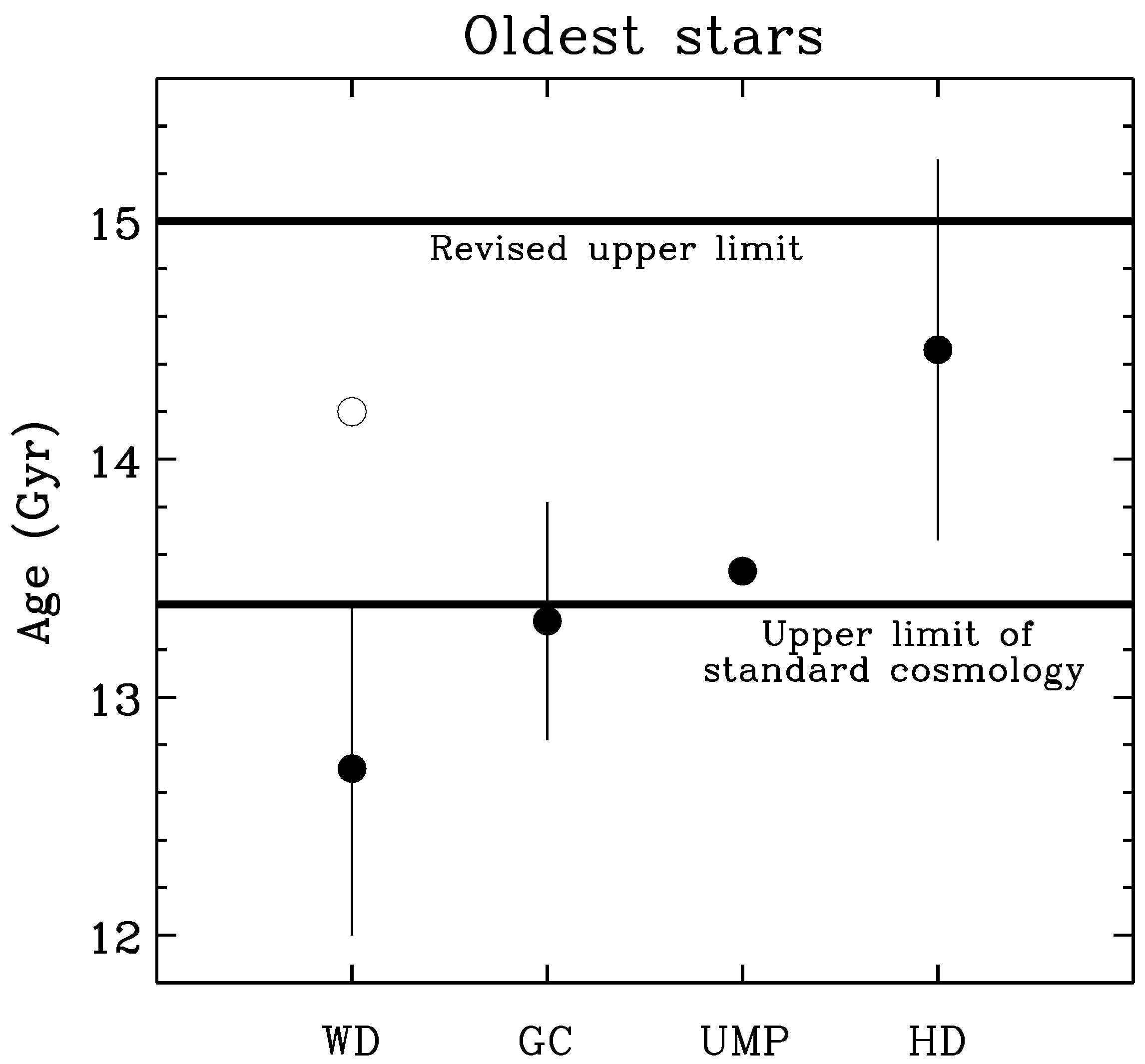
With the present theory, the age of the universe is increased from 13.8 Gyr to 15.4 Gyr. This relieves some tension with the determined stellar ages for some of the oldest known stars. The error bars of stellar ages, however, need to be reduced before this difference can be used as a suitable cosmological test.

An observational validation of the theory is, however, already available: The theory resolves the $H_0$ tension and predicts its observed magnitude without the use of any free parameters. When the cosmological constant is removed from the equation for the $a\left(t\right)$ function that is used by standard cosmology in the CMB analysis, the systematic difference between the value of the Hubble constant $H_0$ determined from the redshifts of supernovae and the value determined from modeling of CMD data disappears. Therefore, consistency of cosmological theory is restored.

While this kind of explanation of the cosmological constant and the $H_0$ tension has been given by the present author before (see [29], which also contains references to earlier versions of the theory), the difference is that the previous versions depend on a perturbation approach and arguments from quantum physics. Thus, possible boundary conditions for metric fluctuations constrained within the finite time-frozen 3D subspace that represents the observable universe were explored. The requirement that there should be no observable gravitational effects from such metric vacuum fluctuations was shown to be satisfied by a discrete set of fluctuation modes. Each mode corresponds to a boundary term that formally appears as a cosmological constant. If one makes use of arguments from quantum physics that the universe should be in the mode with the lowest allowed energy state, then a unique value for the constant $\Lambda$-type boundary term is obtained. It is found to agree with the observationally determined value for the cosmological constant, without the use of any free parameters in the theory.

In contrast, the present version of the theory does not make use of any perturbation analysis or heuristic arguments from quantum physics. The derivation is entirely classical.