
Article

Segmentation of Crop Residue Using an Open-Source Labeling Tool with U-Net and DeepLabV3

Department of Agricultural and Biological Engineering, The Grainger College of Engineering, College of Agricultural, Consumer, and Environmental Sciences, University of Illinois Urbana-Champaign, 1304 W, Pennsylvania Avenue, Urbana, IL 61801, USA
*
Author to whom correspondence should be addressed.
AgriEngineering 2026, 8(6), 228; https://doi.org/10.3390/agriengineering8060228
Submission received: 8 April 2026 / Revised: 26 May 2026 / Accepted: 30 May 2026 / Published: 5 June 2026
(This article belongs to the Special Issue The Future of Artificial Intelligence in Agriculture, 2nd Edition)

Abstract

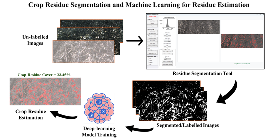
Crop residue management is an important factor in sustainable agriculture as it impacts soil erosion, water retention, soil organic matter, and crop yield. Accurately measuring the crop residue cover helps in the strategic planning, control, and monitoring of crop residue. While advancements in machine learning have allowed for significant progress in crop residue classification work, a major challenge still exists in the creation of an accurately annotated dataset for crop residue and the application of segmentation-based models to accurately segment crop residues. This study aims to develop an efficient image annotation framework and evaluate deep learning models for crop residue cover estimation. For this, the Residue Segmentation Tool, a standalone graphical user interface, was designed to facilitate accurate and efficient image annotation that enables flexible and high-throughput annotation of residue images. The tool is publicly available and supports multiple segmentation modes, which include classical and modern computer vision algorithms such as Otsu, Canny, and manual thresholding, as well as the Segment Anything Model and user-guided mask refinement through manual editing options. This tool was also utilized to create annotated datasets for machine learning training and testing of crop residue cover estimation. Three different sizes of datasets (100, 250, and 500 images) were utilized for machine learning training and testing to evaluate the performance of the models trained using U-Net and DeepLabV3. U-Net consistently outperformed DeepLabV3 across most metrics, particularly on smaller datasets, showing better Dice, IoU, and Recall scores. The best-performing model had Dice, IoU, and Accuracy scores of 0.748, 0.627, and 0.864, respectively. The findings demonstrate that the Residue Segmentation Tool enables scalable and reproducible dataset creation and supports effective segmentation for crop residue cover estimation.

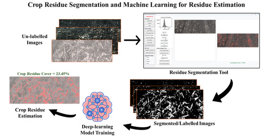
Graphical Abstract

1. Introduction

One essential aspect of sustainable agriculture is the efficient management of crop residues, which have significant implications for soil health, greenhouse gas emissions, and nutrient cycling [1,2]. Accurate estimation of crop residues can help in the development of targeted and efficient strategies for their utilization, recycling, and disposal. Traditional methods of crop residue cover measurement such as the line-transects method or visual assessment method are limited by subjectivity, low accuracy, and variability between observers. More modern methods utilize photographic methods [3,4,5,6,7,8] as ground truth data coupled with machine learning methods for the classification of residue into different levels of crop residue cover [9,10,11,12,13,14]. A more accurate way of crop residue estimation is pixel-wise classification of individual pixels in the image as crop residue or soil [15]. However, annotating each pixel using currently available open-source image processing tools, such as Fiji [16], or semi-automated proprietary tools, such as MATLAB’s super pixel-based labeling in the Image Processing Toolbox, has limitations in terms of time and training required and access to the software platforms for labeling. Other web-based public access platforms for data annotation can pose privacy/data-control concerns. More recent open-source annotation platforms such as LabelMe, CVAT, and LabelStudio offer scalable labeling environments and support for modern workflows, including integration with deep learning models. However, these tools are generally designed for broad, multi-class annotation tasks and often require additional configuration or manual intervention when applied to fine-grained, binary segmentation problems such as crop residue detection. To bridge this gap, this study introduces the Residue Segmentation Tool, an interactive standalone open-source graphical user interface (GUI) that combines classical computer vision techniques and deep learning-based segmentation to support researchers in labeling residue imagery. Built with a user-friendly interface, this tool allows users to create high-quality segmentation mask datasets for residue or other binary segmentation tasks. By focusing on domain-specific requirements such as handling fine, discontinuous residue patterns and simplifying the annotation process, the tool reduces labeling complexity while maintaining accuracy.
Despite the lack of a domain-specific segmentation tool for crop residue cover segmentation, there have been a few research attempts on the application of segmentation-based approaches for pixel-wise classification of crop residue. Initial attempts at segmentation-based classification of image pixels into soil, residue, and plants, such as work on using object-based image analysis for soil cover type, relied on manual adjustment of parameters [17]. Riegler-Nurscher et al. (2018) utilized entangled random forest, a machine learning approach, for pixel-wise classification of residue and vegetation cover from images captured in diffuse (cloudy) light conditions with no direct sunlight [15]. For data annotation, they used Simple Linear Iterative Clustering (SLIC), proposed by [18], on cropped images from high-resolution images. The size of super-pixels and color similarity were adjusted on a user interface with only three sliders to set the parameters and object class for a recursive clustering-based pre-segmentation [15]. Gao et al. (2024) developed a deep learning model, ‘CCRSNet’, for segmentation of crop residue from field images [19]. This study utilized tightly cropped images of size 256 × 256 captured in orthogonal orientation to create segmented labels using the Labelme annotation platform introduced by [20]. While a high-performance score was reported in this study, such tightly cropped and orthogonal views simplify the visual distinction between crop residue and soil. This is an advantage that is commonly not available in on-machine sensing situations where solutions must work with wider-view oblique images. Objects in images with oblique views have relatively larger scale variation compared to scenes captured in orthogonal images, which limits the performance of deep neural networks that process images in a single-scale fashion [21]. Li et al. (2021) utilized oblique images of crop residues for their research work on application of the Siamese Domain Transfer Network (SDTN) for residue detection, where the highest observed average precision (AP) was 51.20% [22]. With the advancement of computer vision and deep learning techniques, there is potential to utilize state-of-the-art deep learning segmentation models in crop residue for more accurate and automated estimation in images that capture a diversity of image conditions such as lighting conditions, scale of resolution, soil background, and oblique images with different oblique view angles.
U-Net [23] and DeepLabV3 [24], both state-of-the-art deep learning segmentation models, are increasingly being used in several agricultural applications such as estimation of crop damage by wildlife using U-Net on drone images [25], quantifying the consistency of crop establishment using U-Net [26], estimation of tree canopy closure using U-Net [27], corn straw return detection using Sh-DeepLabv3+ built upon the DeepLabV3 architecture [28], and corn straw plot classification using GCF-DeepLabv3+ built upon the DeepLabV3 architecture [29], to mention a few. These two models are well-suited for handling fine-grained segmentation of crop residues due to their demonstrated efficiency in handling high-resolution, fine-structured segmentation tasks. These architectures offer competitive performance at lower inference costs than recent transformer-based or instance-segmentation approaches. However, to the best of our knowledge, there has been no study on the utilization of these models for segmentation-based quantification of crop residue cover using high-resolution oblique images.
Therefore, the objective of this research is to (a) develop a customized open-source data annotation tool—the ‘Residue Segmentation Tool’—for image segmentation work and (b) utilize the labeled dataset from the Residue Segmentation Tool to segment crop residue cover using state-of-the-art deep learning approaches of U-Net and DeepLabV3. The Residue Segmentation Tool will help researchers create segmentation masks for machine learning training, and the results of the ML training will provide valuable insight into the usability of segmentation-based deep learning architecture in correctly estimating crop residue cover. This research utilizes real-world images captured from on-machine sensors during actual tillage operations under varying lighting conditions, resolutions, and oblique angles. These factors introduce significant variability and noise, making the task of crop residue segmentation more representative of field conditions and substantially more challenging.

2. Materials and Methods

2.1. Data Collection

The image data used for this study was collected using tractor and tillage implement-mounted on-machine camera sensors during both fall and spring tillage data collection for the years 2022 to 2024. The image data consists of corn residue obtained from on-machine data collection in various fields in Illinois and Iowa. These images come from different hardware sensors mounted at different heights or angles, giving a diversity of images in terms of obliqueness, resolution, color, contrast, light conditions, and soil background. Images were collected from the front of the tractor and rear of the implement during both active and idle tillage passes, with an idle pass referring to the situation when camera sensors were collecting data from tractors and implements without actually tilling the fields. For spring 2023, a camera system was mounted on the rear of an ATV to collect images during idle passes. To capture different variations of the residue images, the images used in this study come from 29 different fields and capture different lighting conditions ranging from early morning to late evening to capture diverse lighting effects, different image resolutions, and different oblique angles that were intentionally varied across different collection seasons to enhance the diversity of the perspective angles in the dataset. While this data collection led to thousands of images from multiple fields, a strategically selected subset of images is used in this study, ensuring that images from each of the fields are included in the dataset. This was done due to the constraint on resources and time for labeling the dataset, while making sure that the variations in images across fields, camera hardware, soil background, and lighting conditions were captured. The final dataset consists of 500 images collected across 29 distinct field environments.

2.2. Residue Segmentation Tool

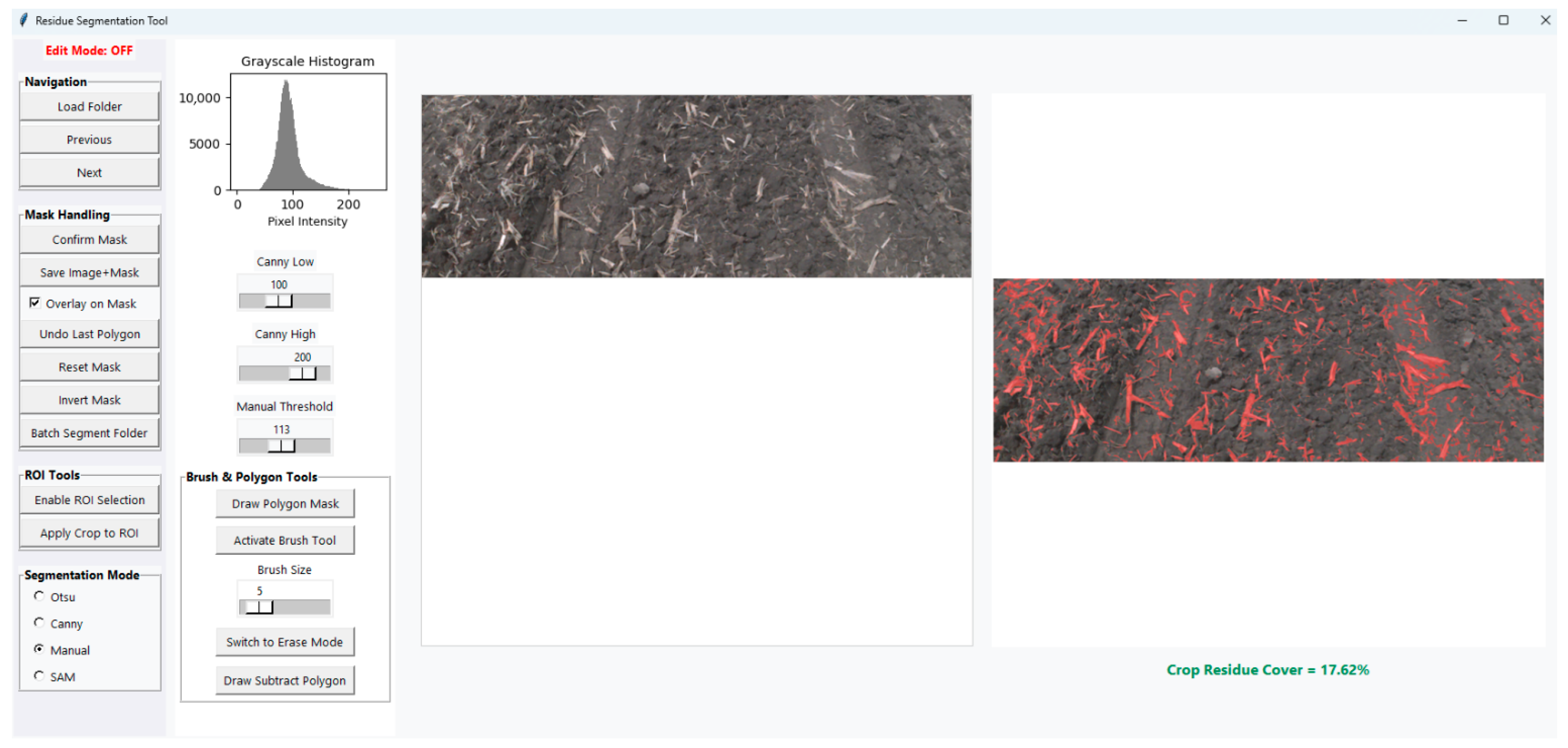
The Residue Segmentation Tool was developed using Python v3.12 with Tkinter for the graphical user interface (GUI), OpenCV v4.10.0 for image operations, and PyTorch v2.5.1 for integrating the Segment Anything Model (SAM) v2. Modular controls for navigation, segmentation, annotation, and export were added to the application architecture. Figure 1 shows the graphical user interface of the Residue Segmentation Tool. The tool, along with the necessary files, and a video demonstration are made available publicly. This tool is standalone and can simply be downloaded and run on any computer.
There are four segmentation modes available in the tool, and users can manually select and switch between these modes through the GUI (with Otsu thresholding used as the default initialization):
(1)
Otsu thresholding [30] automatically determines a binary threshold by maximizing inter-class variance in grayscale histograms. This method is a default setup in the Residue Segmentation Tool.
(2)
Canny edge [31] applies edge detection, followed by a 3 × 3 kernel morphological opening and cleaning to generate a binary mask.
(3)
Manual thresholding allows users to manually select a grayscale threshold for segmentation.
(4)
SAM (Segment Anything Model) implements Meta AI’s pretrained SAM [32] with a ViT-b backbone. The full image is submitted as a bounding box for SAM to automatically generate a residue mask (i.e., no interactive prompting such as point clicks is used). SAM supports more advanced prompting strategies such as point-based or grid-based prompting. However, these were not explored here as the focus of this work is not on prompt engineering but on comparative segmentation performance under standardized conditions. Also, ViT-b backbone has lower computational requirements compared to other variants such as ViT-l and ViT-h.
To fine-tune the initial binary mask generated by the above four methods, manual annotation and mask editing options are also included in the tool. To refine automatic masks, users can interactively draw (or undo) polygon annotations to add or subtract regions from the mask. The tool also allows users to use a brush/eraser tool for pixel-wise editing with adjustable brush size (controlled via a GUI slider). Automatically segmented images sometimes confuse foreground with background, and hence the ‘Invert Mask’ option of the tools is designed to invert the mask (i.e., move the foreground pixels to the background, and vice versa). The tool also allows cropping based on the region-of-interest (ROI) selection. A live histogram plot of grayscale intensities aids in visual decision making. Finally, the save and export section of the tool allows final masks to be saved alongside the corresponding images for use in machine learning (ML) training datasets. This tool also allows batch segmentation of all images within a selected folder, generating structured outputs for downstream processing. Table 1 summarizes the main features of the Residue Segmentation Tool.

2.3. Data Preprocessing for ML Training

The images, which were of sizes 1200 × 400, were segmented using the Residue Segmentation Tool by two annotators: the first author and an undergraduate researcher. To ensure annotation consistency, all outputs from the undergraduate annotator, who annotated nearly 200 images, were systematically reviewed and validated by the first author prior to inclusion in the final dataset. Validation consisted of visual inspection of segmentation completeness, boundary consistency, and correction of inaccurate or incomplete masks if necessary. The tool output both the input images and segmented images with the same names in parallel folders to ease the data loading process during machine learning training. The segmented images were organized into three different dataset sizes (100 images, 250 images, and 500 images) for machine learning training to evaluate the effect of training size on model performance. Each dataset was split into training, validation, and test sets in a 70%, 15%, and 15% ratio, respectively. To facilitate a comparable study between the two models tested, a fixed seed was used for the Python random module, the Numpy random module, PyTorch CPU and CUDA random numbers, and deterministic behaviors in the models required to train the models. This ensured that the same training split was obtained for both models, the same order of shuffling was maintained in the data loaders, the same model weights were initialized for different trainings, and the same gradient and optimizer behavior was preserved as much as possible. However, this does not guarantee an exact sequence of training or that the same exact images are tested for each model because PyTorch CPU and CUDA behavior can be non-deterministic, floating-point operations are subject to precision errors, and there can be other system noise. Images used for model training were 1200 × 400 pixels. Pixel values were normalized to the range [0, 1] using PyTorch’s tensor conversion. Corresponding segmentation masks were converted to grayscale, resized to the same resolution, and binarized using a threshold of 0.5 to ensure consistent class representation. No additional padding or mean standard deviation normalization was applied. A fixed input resolution was maintained across all experiments to ensure consistent receptive field behavior. During the final training of the models, no data augmentation was done on the image datasets. This was because a preliminary study with a dataset of 175 training and 38 test images showed similar results for IoU and Dice Coefficient with and without data augmentation. The applied data augmentation during the preliminary study included RandomRotation(30), RandomHorizontalFlip (p = 0.5), ColorJitter, RandomAffine, and RandomPerspective. This preliminary study was conducted on both UNet and DeepLabV3 models.

2.4. Deep Learning Models

For the segmentation-based machine learning for crop residue cover estimation, two CNN architectures were used in this study: U-Net and DeepLabV3. Both models were implemented using the PyTorch framework [33]. U-Net was originally developed for biomedical image segmentation. Its fully convolutional network architecture follows a symmetric encoder–decoder structure with skip connections between the corresponding encoder and decoder paths [23]. In this study, a 3-level U-Net (comprising two encoder levels and a bottleneck) was implemented, starting with 64 initial filters, without the use of batch normalization or dropout layers. DeepLabV3 is another state-of-the-art model for semantic segmentation that uses atrous (or dilated) convolutions, a technique that allows it to capture context information at different scales [24] without increasing the complexity of the model. In this study, DeepLabV3 with a ResNet-50 backbone and U-Net were both models trained from scratch on the residue dataset created using the Residue Segmentation Tool. DeepLabV3+ extends DeepLabV3 by incorporating an explicit decoder module designed to improve segmentation and recover fine-scale spatial detail [34]. While this variant has demonstrated enhanced performance in several recent agricultural segmentation studies [28,29], the present work deliberately employs DeepLabV3 without the decoder component. This choice was made to preserve a clear architectural separation between the two evaluated paradigms: U-Net, representing an encoder–decoder architecture with skip connections for multiscale feature fusion [23], and DeepLabV3, representing a context aggregation framework based on atrous spatial pyramid pooling without an explicit decoding pathway. This controlled experimental design enables a more direct comparison of these two fundamental segmentation strategies. The omission of DeepLabV3+ is acknowledged as a limitation, particularly with respect to tasks requiring refined boundary reconstruction [34]. The entire architecture was built from basic building blocks since this study deals with a specific domain of crop residue that is very different from the ImageNet dataset that was initially used to train ResNet models, which serve as the backbone for both U-Net and DeepLabV3. Both models were trained and tested using the same dataset with a fixed random seed during the train–test split to ensure a fair comparison as much as possible.

2.5. Model Evaluation Metrics and Accuracy Criteria

In this work, the following standard semantic segmentation evaluation metrics were used to assess model performance on residue segmentation: Dice Similarity Coefficient (Dice), Intersection over Union (IoU), Accuracy, Precision, Recall, and F1 Score [35]. True positives (TP) represent pixels correctly classified as residue; false positives (FP) are pixels incorrectly classified as residue when they are actually soil; false negatives (FN) are residue pixels missed by the model and classified as soil; and true negatives (TN) are correctly classified soil pixels.
All metrics were calculated using binarized predictions (threshold > 0.5). The Dice coefficient, which measures the overlap between predicted and ground truth masks, is defined as:
D i c e = 2 × T P 2 × T P + F P + F N
In other words, the Dice coefficient measures how well the predicted residue regions overlap with the ground truth residue regions. A higher Dice coefficient means that the predicted crop residue closely matches the annotated residue in both extent and shape. Similarly, IoU (also referred to as the Jaccard Index), which measures the intersection area divided by the union area of predicted vs. ground truth masks, is calculated as:
I o U = T P T P + F P + F N
IoU is similar to Dice but penalized more for false positives and negatives, and hence the Dice coefficient is generally higher than IoU. In other words, IoU quantifies the overlap between predicted and actual residue pixels relative to their union, and IoU is stricter than Dice as it penalizes both false residue predictions (FP) and missed residue predictions (FN) [36].
Accuracy measures overall pixel-level correctness (all correctly classified pixels—both soil and residue) and can sometimes be misleading, specifically in imbalanced datasets where the background may dominate (for example, images with lower CRC in the case of crop residue, since predicting most pixels as soil may still yield high accuracy even with poor residue detection). Accuracy is calculated as:
A c c u r a c y = T P + T N T o t a l   n u m b e r   o f   p i x e l s
Precision is another evaluation metric that calculates how many predicted positives are correct. In this problem, precision measures how many of all predicted residue pixels are truly residues. Precision is calculated as:
P r e c i s i o n = T P T P + F P
Recall shows how many actual positives the model catches out of all actual positives. In this problem, recall measures how many of all actual residue pixels are correctly detected. Recall is calculated as:
R e c a l l = T P T P + F N
F1 score calculates the harmonic mean of precision and recall, and it balances both. In binary segmentation, such as crop residue cover segmentation from soil background, F1 score is equal to the Dice coefficient. F1 score is calculated as:
F 1 = 2 × P r e c i s i o n × R e c a l l P r e c i s i o n + R e c a l l
True positives (TP), false positives (FP), and false negatives (FN) were derived by comparing predicted masks to ground truth masks pixel-wise. In addition, per-image CRC (crop residue cover) percentages were computed as the ratio of foreground pixels to total pixels in each predicted mask.
C R C % = R e s i d u e   p i x e l s T o t a l   p i x e l s × 100 %
The models were evaluated on a held-out test set not seen during training or validation. All evaluation metrics were averaged across the test set. These evaluations are based on region-overlap metrics, which primarily quantify area-based agreement and do not explicitly measure boundary alignment. Potential discrepancies between segmentation overlap and boundary alignment are not directly captured in the present evaluation framework, and this is acknowledged as a limitation of the study.

2.6. Hyperparameter Selection and Statistical Analysis

Model hyperparameters were selected using preliminary tuning experiments on the validation set. Learning rates used in this preliminary tuning ranged from 1 × 10⁻³ to 5 × 10⁻⁵, decreasing by 5 × 10⁻¹. Early stopping was not done during initial training, and a final training with 100 epochs was chosen as the validation accuracy plateaued around 100 epochs. The final configuration was chosen based on stable convergence and optimal validation performance across architectures. The selected hyperparameters were:
  • Number of epochs = 100
  • Optimizer = Adam
  • Loss functions = Dice Loss and BCE Loss (equal weighting),
  • Learning rate = 1 × 10⁻⁴
  • Activation function = Sigmoid (applied to model outputs for binary segmentation)
  • Threshold for mask = 0.5 (used to binarize the predicted probability masks)
  • Random seed = 42 (to ensure reproducibility between two models)
To mitigate the challenges of class imbalance, a combined Dice and Binary Cross-Entropy (BCE) loss function was utilized. This approach leverages the robustness of Dice loss to handle spatial overlap while BCE helps stabilize gradient flow.
Statistical analysis was conducted using mixed-effects regression models and non-parametric Wilcoxon signed-rank tests to evaluate segmentation performance differences between U-Net and DeepLabV3 architectures across three training dataset sizes (70, 175, and 350 images), accounting for subject-level variability in the repeated measures design with 75 paired observations (test images) per condition. For all mixed-effects models, the underlying statistical assumptions were verified by inspecting the normality of residuals and assessing homoscedasticity.

3. Results and Discussion

3.1. Assessment of Residue Segmentation Tool

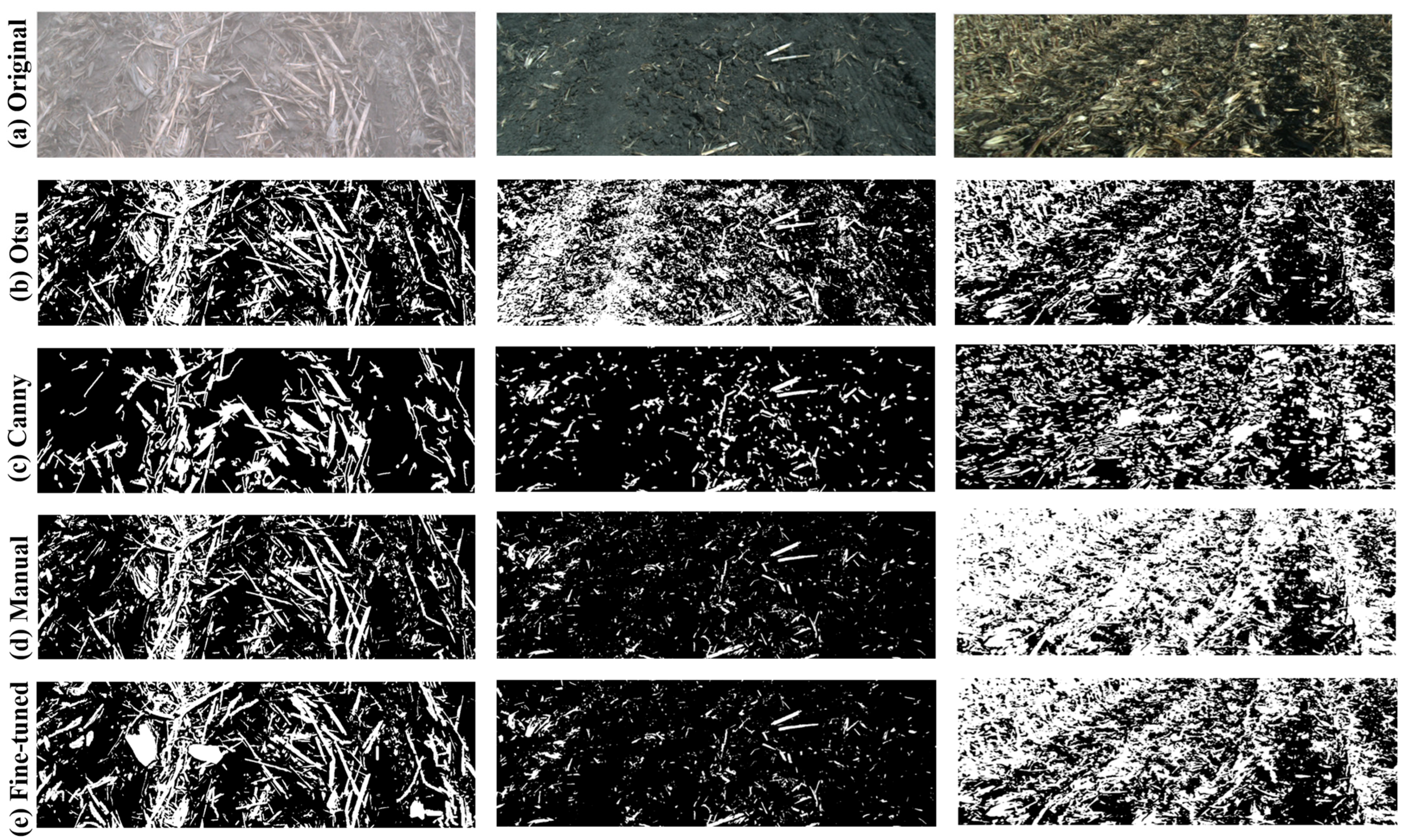
To evaluate the effectiveness of datasets created using the Residue Segmentation Tool, a visual assessment was done by comparing the segmentation mask created using different segmentation modes and the final mask generated after using the manual mask editing tools (polygon and/or brush tools), as shown in Figure 2. The Residue Segmentation Tool significantly reduced the time and complexity involved in creating the labeled segmentation dataset for crop residue estimation work. Using this tool, it took between 10 s and 180 s to label a single image, depending on the amount of residue, colors and brightness, and the angle of obliquity present in the input image. The tool’s modular design, support for multiple segmentation modes, and export-ready format for segmentation datasets make it ideal not just for crop residue cover but also for other computer vision tasks requiring binary mask segmentation.

3.2. Model Performance on Residue Segmentation

Model training was done at three different dataset sizes—100 images, 250 images, and 500 images in total. Briefly, 70% of this dataset was used for training, 15% for validation, and the last 15% was used for initial model testing. However, to maintain a consistent comparison, the same set of 75 test images was utilized to evaluate model performance. The 75 test images constitute a fixed, fully held-out set that was excluded from training and validation across all dataset sizes (100, 250, and 500 images), ensuring that no data leakage occurred in any experimental condition.

3.2.1. Training and Validation Loss and Accuracy

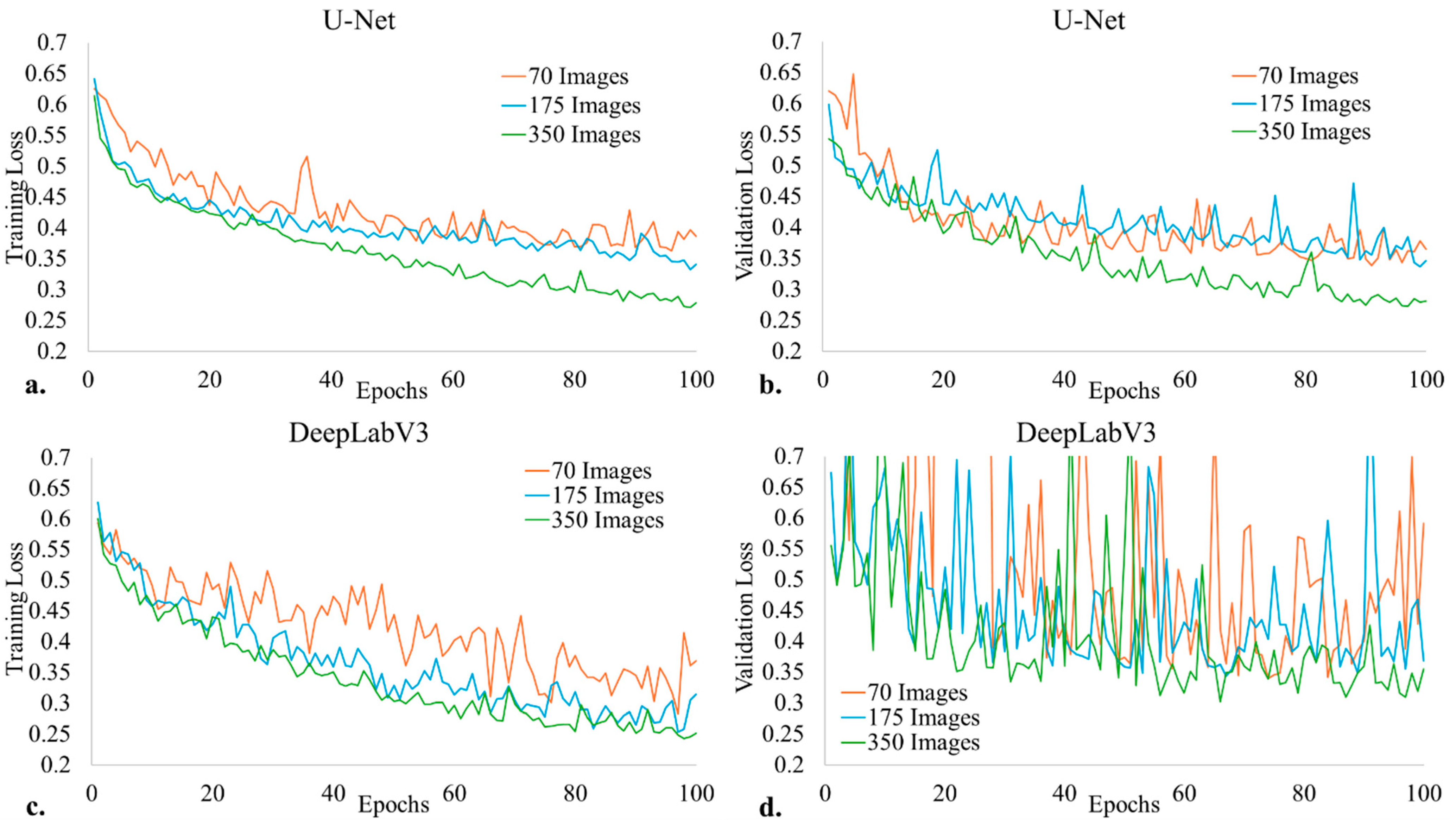
Training loss curves indicated stable convergence in both models, with U-Net demonstrating improved convergence with increased training data—as shown in Figure 3, where the training loss curves for U-Net became smoother with lower training loss for larger datasets. Similar trends were observed with validation loss for U-Net, where higher and more fluctuating validation loss occurred in smaller datasets. DeepLabV3 showed robust training dynamics across dataset sizes with lower training loss after 100 epochs compared to the training loss from U-Net at each dataset size. Despite strong training performance, DeepLabV3 showed volatile validation loss across all dataset sizes (Figure 3), indicating potential overfitting or sensitivity to validation data.
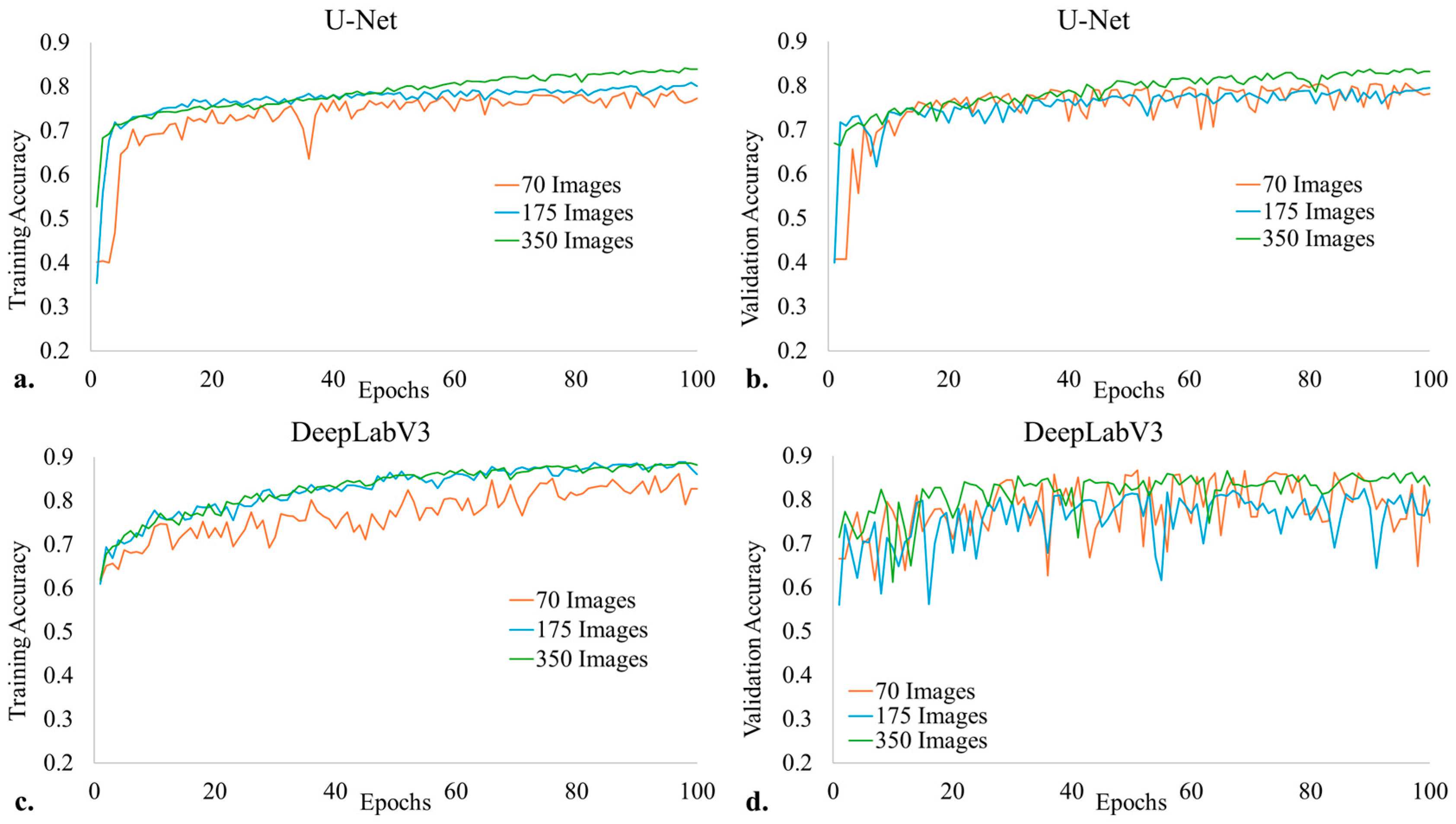
Training and validation accuracy curves for DeepLabV3 and U-Net across growing dataset sizes are shown in Figure 4. With more training data, U-Net demonstrated a consistent increase and convergence in training and validation accuracy, indicating its capacity to generalize well with sufficient data. Even with larger datasets, DeepLabV3 showed notable variations in validation accuracy despite maintaining excellent training accuracy, especially in the early training stages. This indicates that whereas DeepLabV3 could be sensitive to validation conditions or prone to overfitting, U-Net could offer more dependable and consistent generalization performance.

3.2.2. Testing Accuracy on Crop Residue Segmentation

Both U-Net and DeepLabV3 models successfully segmented residue from the background in high-resolution images. Quantitative evaluation (Table 2) showed that U-Net consistently outperformed DeepLabV3. Across all dataset sizes, U-Net achieved higher scores in Dice coefficient, IoU, and Recall. This result is consistent with the loss/accuracy during model training, suggesting that U-Net generalized better for crop residue cover images. With the increasing dataset, U-Net improved in Dice (from 0.634 to 0.748) and IoU (from 0.517 to 0.627). Dice and IoU also increased for DeepLabV3; however, they started lower and ended lower. With more data, DeepLabV3 demonstrated notable improvements, although it never entirely achieved U-Net’s level of performance. The slight increase in standard deviation at DS = 350 for the Dice coefficient could be due to the inclusion of a few challenging test images that influenced model performance. DeepLabV3 showed notable trade-offs between precision and recall, especially for smaller dataset sizes, but U-Net’s recall remained high across all sizes, indicating its superior ability to detect important regions. U-Net showed more stable performance (lower standard deviations in some cases) and better overall segmentation quality, making it a more suitable model for crop residue segmentation. The accuracy obtained in this study is comparable to the findings of [19], where they obtained a maximum accuracy of 93.54% using their customized CCRSNet on cropped orthogonal images of 256 × 256 size. Our study reported a mean accuracy of 86.4%, with the highest accuracy reaching up to 97.7% on oblique images, which represent a more challenging and realistic imaging scenario.
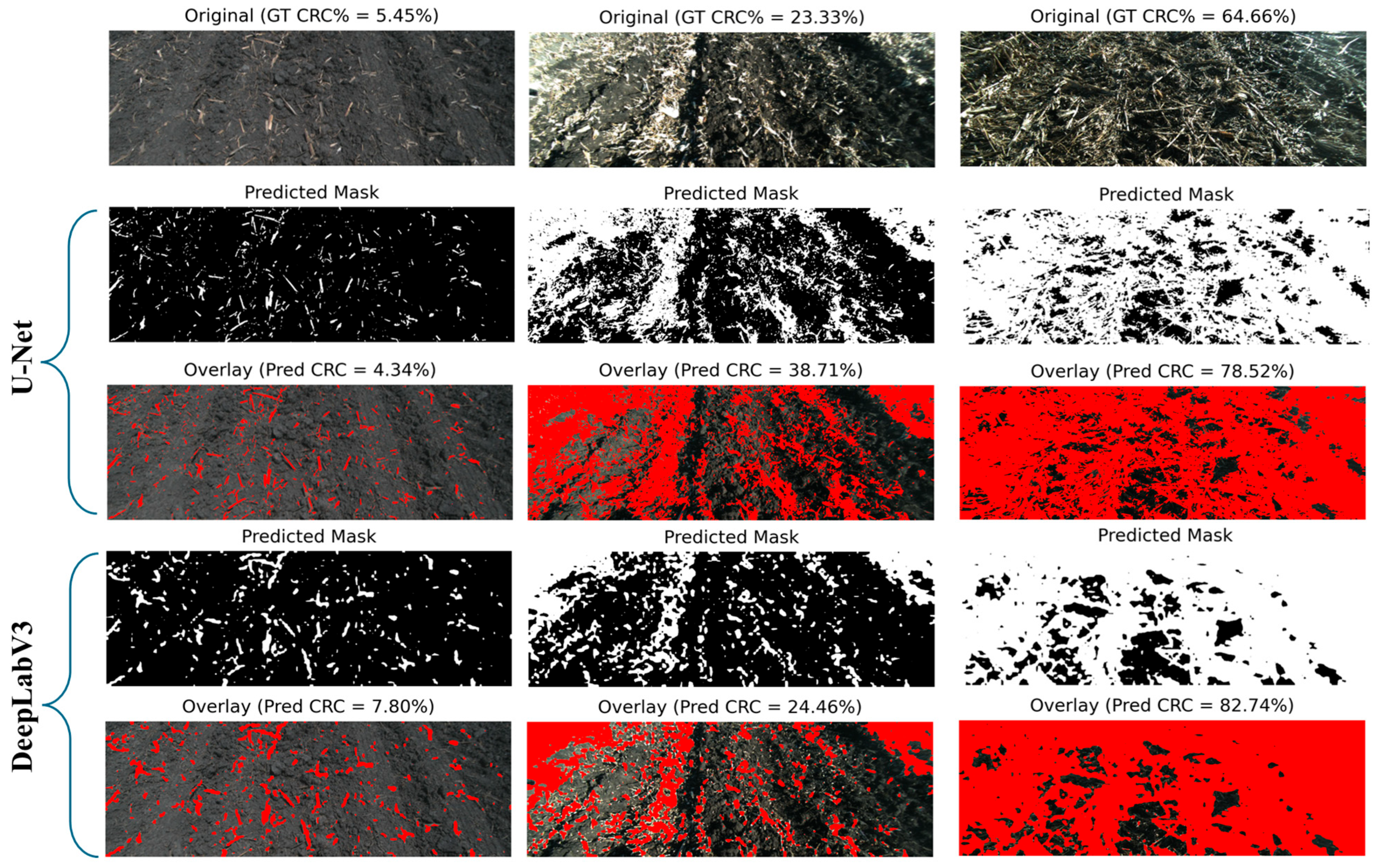
Visual inspection of predicted segmentation masks and manually annotated ground truth masks demonstrated a high degree of spatial agreement across all model configurations in most cases. As shown in Figure 5, both U-Net and DeepLabV3 architectures trained with 350 images were able to accurately highlight crop residue regions at different residue levels, soil background, and color contrasts. This qualitative agreement supports the quantitative results and indicates that the models can capture relevant spatial patterns rather than relying solely on pixel-level accuracy. The ability to maintain segmentation quality under heterogeneous field conditions is particularly important for practical agricultural applications, where variations in soil texture, illumination, and residue distribution are common.
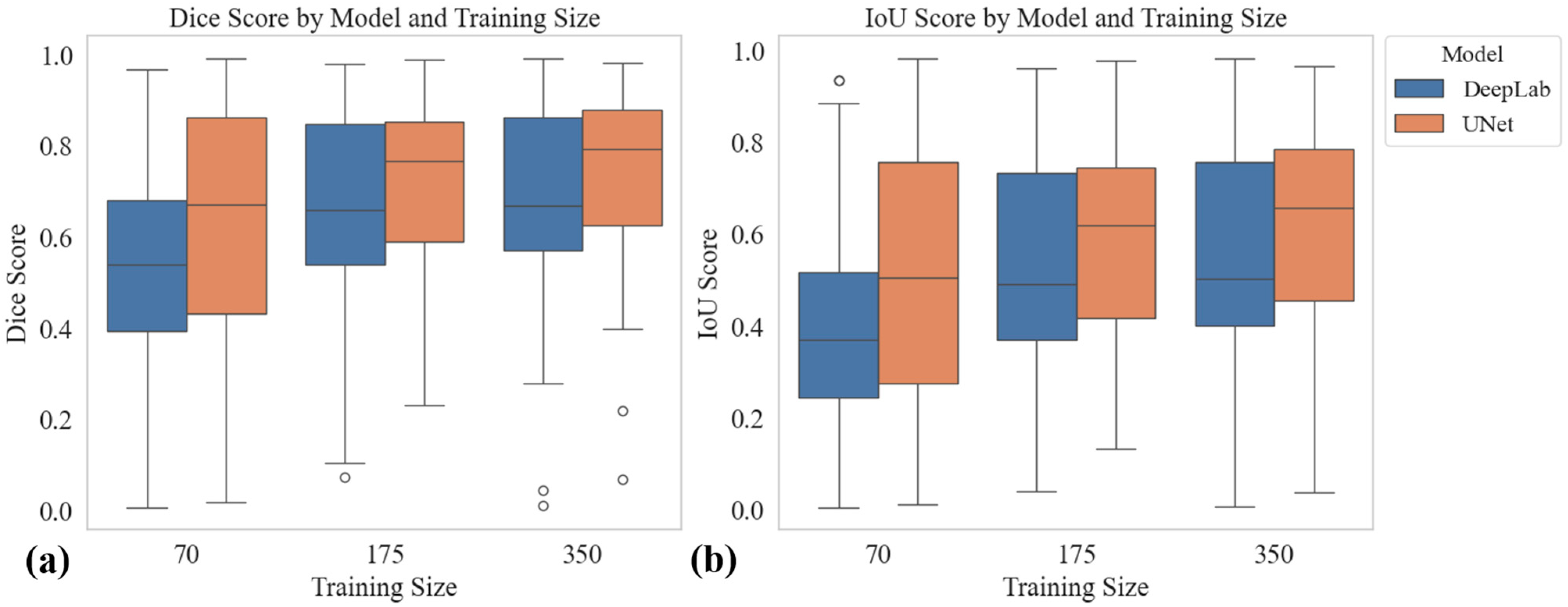
The average scores reported in Table 2 can be further analyzed by plotting the distribution of individual test image score performance to compare the overall variation between the two models at three different dataset sizes. Figure 6 shows the boxplot of the distribution of the Dice score (which is equal to the F1 score in this case of a binary segmentation problem) and IoU. Both DeepLabV3 and U-Net showed higher median Dice scores as the training size increases. At every dataset size, U-Net’s median Dice is consistently higher than DeepLabV3’s. DeepLabV3 struggled more with the lower dataset, and as the dataset increased, DeepLabV3 had improved scores. Like the Dice score, both models showed increased median IoU when moving from 70 images in the training dataset to 350 images in the training dataset, and U-Net had higher median and more consistent IoU scores at the larger training size. The DeepLabV3 model trained with 70 images had a median IoU score of only 0.38, indicating instability and confirming the trends in validation loss seen during the model training in Figure 3. Although IoU for DeepLabV3 improved with more data, it still lags behind U-Net in both mean and consistency. The observed performance differences between U-Net and DeepLabV3 are likely influenced by the characteristics of the crop residue segmentation task rather than a general superiority of one architecture over the other. Crop residue in high-resolution field imagery typically appears as thin, discontinuous, and high-frequency texture patterns with weak global structure. In such cases, U-Net’s encoder-decoder design with skip connections facilitates the preservation of low-level spatial details during up-sampling, which is critical for accurate segmentation of fine residue boundaries. DeepLabV3 relies on atrous spatial pyramid pooling to capture multi-scale contextual information, which is more effective for objects with larger and more homogeneous spatial extents. This architectural difference may explain the relatively lower performance observed for DeepLabV3 in this dataset.
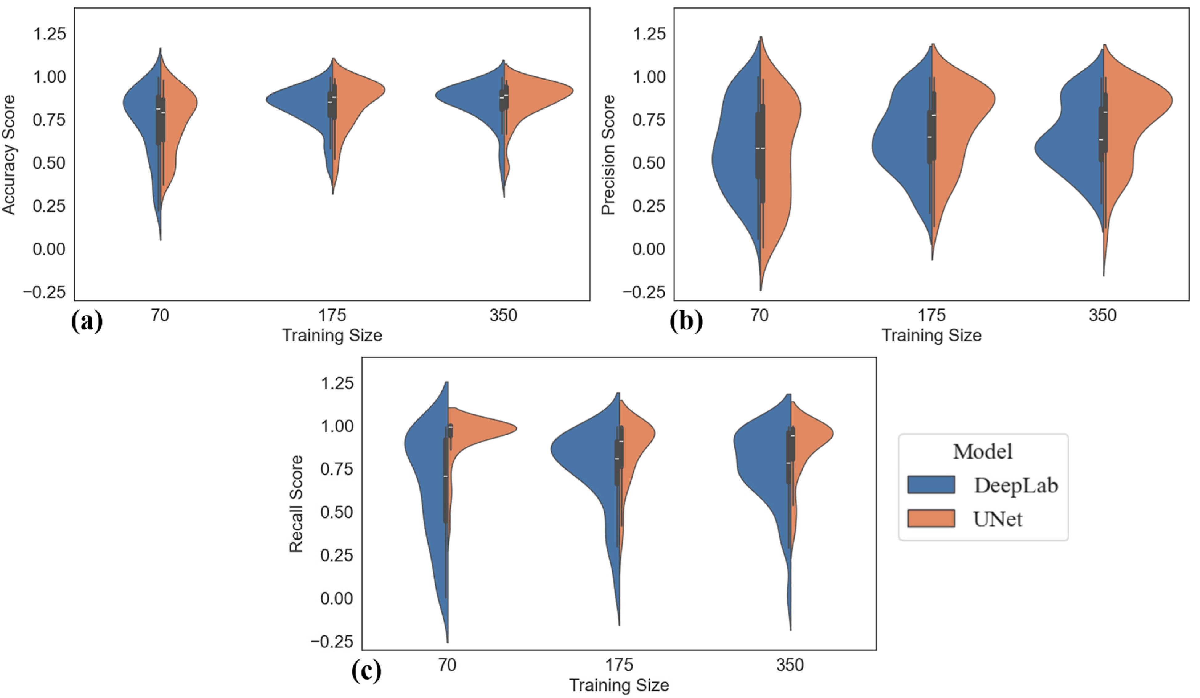
U-Net demonstrates more consistent and generally superior performance than DeepLabV3 across dataset sizes, particularly for recall and precision. Figure 7 shows the distribution of individual image performance across two models and different dataset sizes using violin plots for the remaining performance metrics—Precision, Accuracy, and Recall. The use of violin plots effectively conveys the distribution and spread of scores, which is valuable for understanding not only the central trends but also the model consistency across repeated runs. Across all metrics and training sizes, U-Net demonstrates more consistent and often superior performance, especially noticeable in recall, where the distributions are generally tighter and centered around higher values compared to DeepLabV3. DeepLabV3 exhibits greater variability, particularly with smaller training sizes, indicating it may be more sensitive to limited data. As training size increases, both models show performance improvement and reduced variability, but U-Net consistently maintains a slight edge or parity.
Mixed-effects models revealed statistically significant main effects of both model type and training size for the Dice coefficient (LR = 43.55, p = 1.88 × 10⁻⁹; LR = 79.51, p = 2.21 × 10⁻¹⁶) and IoU (LR = 43.47, p = 1.96 × 10⁻⁹; LR = 79.46, p = 2.27 × 10⁻¹⁶), while precision exhibited a significant model-by-training size interaction (LR = 23.89, p = 6.49 × 10⁻⁶). Wilcoxon signed-rank tests consistently demonstrated U-Net’s superior performance over DeepLabV3 across all training sizes for Dice (median improvements: 0.132–0.125, p < 0.001) and IoU (median improvements: 0.136–0.156, p < 0.001), with small but consistent effect sizes (Cliff’s delta: 0.177–0.224). U-Net also showed substantial advantages in recall, particularly at the smallest training size (median difference: 0.288, p = 2.62 × 10⁻¹¹, large effect), while precision differences were modest and training size-dependent. Further investigation of the outliers for Dice and IoU score plots, as shown in Figure 6, revealed that the images with very low CRC values (~1–4%) are associated with the lowest Dice and IoU scores. This is because the overlap-based metrics such as Dice and IoU are sensitive to minor prediction errors. In contrast, high-performing outliers are observed across both low and high CRC ranges, indicating that CRC alone does not fully account for this variability.

3.2.3. Crop Residue Cover Estimation

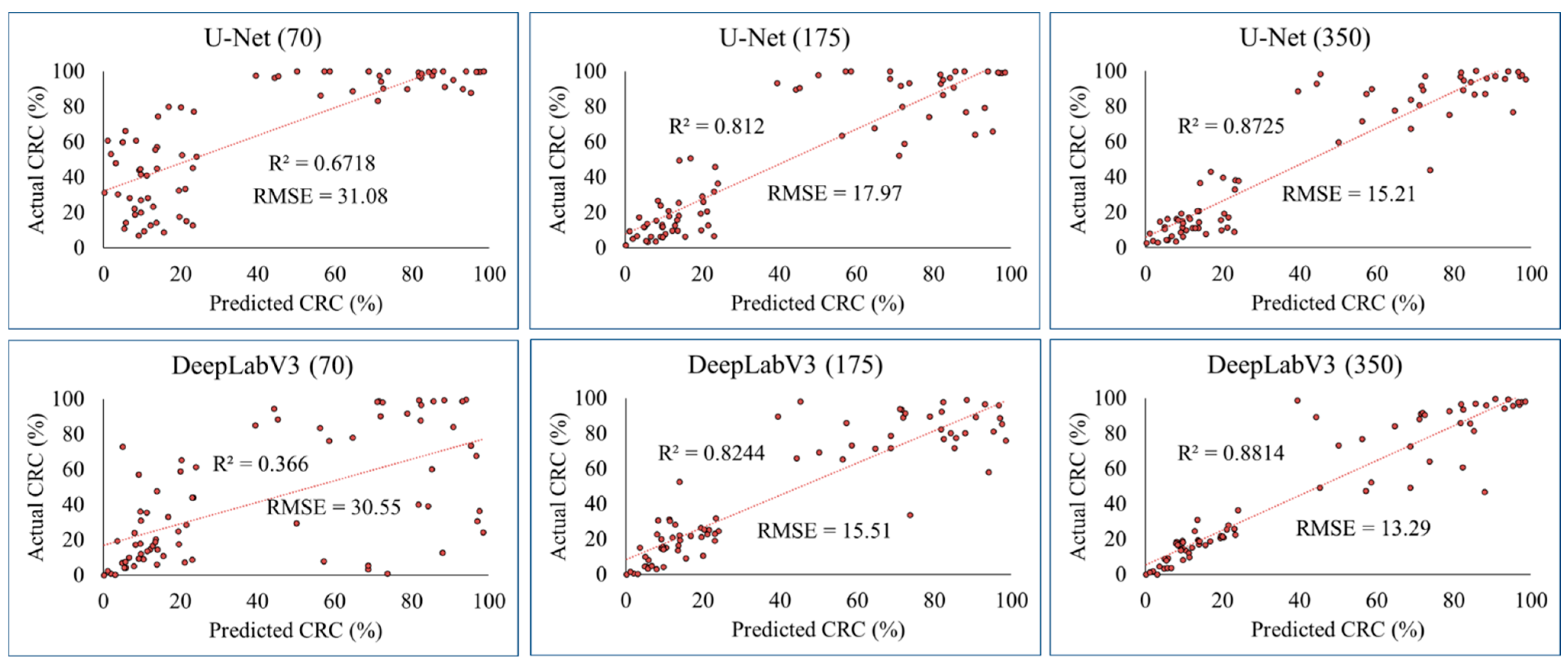
Finally, to estimate crop residue cover percentage, the foreground pixels of the segmented mask were divided by the total image pixels, and that number was multiplied by 100 to get CRC%. To compare the performance of each model on CRC prediction, scatter plots, including a line fit with an R2 value and RMSE, were plotted as shown in Figure 8. To facilitate a comparable discussion, the same set of 75 test images was used in the model CRC predictions. In general, model performance improved with more training data for both U-Net and DeepLabV3, with U-Net and DeepLabV3 having comparable performance in CRC prediction. Both U-Net and DeepLabV3 struggled with small datasets but scaled much better with larger training data, ultimately reaching R2 values greater than 0.87. While some outliers existed, the plots in Figure 8 show increasing tightness around the regression line as the training size increased, as suggested by both increasing R2 and decreasing RMSE values, which show improved prediction accuracy. The R2 values obtained in this study in most cases (except for DeepLabV3 with 70 training image dataset) are higher than the reported R2 value by [15] in classifying the residues (R2 = 0.60) using the Entangled Random Forest method on their super-pixel-based segmentation work. These reported R2 values are also either higher than or comparable to the reported R2 value (R2 = 0.80) by [19] on estimating crop residue in most cases. These results demonstrate the ability of deep learning models to correctly segment the residues and estimate the crop residue cover under various light conditions and soil colors on highly confident labeled image data using the Residue Segmentation Tool. The results presented here demonstrate robust performance on high-resolution, oblique field images, highlighting the effectiveness of the proposed annotation framework and segmentation models for real-world deployment.

4. Conclusions

This study presented a deep learning-based approach to crop residue estimation using the U-Net and DeepLabv3 models. A customized Residue Segmentation Tool was developed for dataset creation and has been made open source. The Residue Segmentation Tool enabled efficient, accurate, and user-friendly annotation of the crop residue dataset for binary segmentation work. The integration of traditional computer vision and modern deep learning makes this tool suitable for researchers and practitioners aiming to develop and evaluate image segmentation models in agriculture by creating ML-ready datasets.
The deep learning-based training showed that both U-Net and DeepLabV3 had strong segmentation performance in segmenting crop residue, with Dice and IoU scores of up to 74.80% and 62.70% (U-Net), and 68.40% and 55.50% (DeepLabV3) respectively. Comparing the ground truth CRC estimation with the model predicted CRC, most models performed well, with R2 values reaching up to 0.88 for the best-performing model. By providing both a data annotation tool and a benchmark segmentation model, this work contributes valuable resources to researchers and practitioners. While this work only considered a total of 500 images coming from diverse backgrounds, with only 350 used for model training, future research can be done on incorporating a larger dataset, including datasets from field locations that are not included in this study. Future research could also explore the possibility of combining datasets from other publicly available resources, as well as including residue from other crops such as soybeans and wheat.

Author Contributions

S.R.: Writing—original draft, reviewing, editing, conceptualization, methodology, investigation, formal analysis, data curation. C.M.A.: Funding acquisition, conceptualization, methodology, supervision, validation, writing—reviewing & editing. All authors have read and agreed to the published version of the manuscript.

Funding

This research was funded by Deere & Company.

Institutional Review Board Statement

Not applicable.

Informed Consent Statement

Not applicable.

Data Availability Statement

The standalone executable application for the residue segmentation tool, along with the tool demonstration video, Python script, and other necessary files, is provided in the following public repository: https://zenodo.org/records/16616012 (accessed on 26 May 2026).

Conflicts of Interest

C.A. has received research grants from Deere & Company. In addition to project funds, the funding sponsor provided instrumentation for the data collection and reviewed the manuscript prior to submission. The funding sponsor had no other roles in the design of this study; analyses or interpretation of data; in the writing of the manuscript; or in the decision to publish the results.

References

  1. Forcella, F.; Buhler, D.D.; McGiffen, M.E. Pest management and crop residues. In Crops Residue Management; CRC Press: Boca Raton, FL, USA, 2018; pp. 173–190. [Google Scholar]
  2. Morrison, J.E.; Huang, C.-H.; Lightle, D.T.; Daughtry, C.S.T. Residue measurement techniques. J. Soil Water Conserv. 1993, 48, 478–483. [Google Scholar] [CrossRef] [Scilit]
  3. Cai, W.; Zhao, S.; Zhang, Z.; Peng, F.; Xu, J. Comparison of different crop residue indices for estimating crop residue cover using field observation data. In Proceedings of the 2018 7th International Conference on Agro-Geoinformatics (Agro-Geoinformatics), Hangzhou, China, 6–9 August 2018. [Google Scholar] [CrossRef] [Scilit]
  4. Hively, W.D.; Shermeyer, J.; Lamb, B.T.; Daughtry, C.T.; Quemada, M.; Keppler, J. Mapping crop residue by combining Landsat and WorldView-3 satellite imagery. Remote Sens. 2019, 11, 1857. [Google Scholar] [CrossRef] [Scilit]
  5. Laamrani, A.; Joosse, P.; Feisthauer, N. Determining the number of measurements required to estimate crop residue cover by different methods. J. Soil Water Conserv. 2017, 72, 471–479. [Google Scholar] [CrossRef] [Scilit]
  6. Laflen, J.M.; Mulla, D.J.; Hintz, E.A. Measuring crop residue cover. J. Soil Water Conserv. 1981, 36, 341–343. [Google Scholar] [CrossRef] [Scilit]
  7. Sullivan, D.G.; Lee, D.; Beasley, J.; Brown, S.; Williams, E.J. Evaluating a crop residue cover index for determining tillage regime in a cotton-corn-peanut rotation. J. Soil Water Conserv. 2008, 63, 28–36. [Google Scholar] [CrossRef]
  8. Yue, J.; Tian, Q.; Liu, Y.; Fu, Y.; Tian, J.; Zhou, C.; Feng, H.; Yang, G. Mapping cropland rice residue cover using a radiative transfer model and deep learning. Comput. Electron. Agric. 2023, 215, 108421. [Google Scholar] [CrossRef] [Scilit]
  9. Ding, Y.; Zhang, H.; Wang, Z.; Xie, Q.; Wang, Y.; Liu, L.; Hall, C.C. A comparison of estimating crop residue cover from Sentinel-2 data using empirical regressions and machine learning methods. Remote Sens. 2020, 12, 1470. [Google Scholar] [CrossRef] [Scilit]
  10. Gao, L.; Zhang, C.; Yun, W.; Ji, W.; Ma, J.; Wang, H.; Li, C.; Zhu, D. Mapping crop residue cover using Adjust Normalized Difference Residue Index based on Sentinel-2 MSI data. Soil Tillage Res. 2022, 220, 105374. [Google Scholar] [CrossRef] [Scilit]
  11. Lima, F.; Blanco-Sepúlveda, R.; Gómez-Moreno, M.L.; Dorado, J.; Peña, J.M. Mapping tillage direction and contour farming by object-based analysis of UAV images. Comput. Electron. Agric. 2021, 187, 106281. [Google Scholar] [CrossRef] [Scilit]
  12. Lory, J.A.; Upadhyay, P.; Lagaunne, T.A.P.; Spinka, C.; Miller, R.; Davis, G.; DeSouza, G.N. Capability of high-resolution RGB imagery to accurately document residue in row-crop fields. J. Soil Water Conserv. 2021, 76, 403–413. [Google Scholar] [CrossRef] [Scilit]
  13. Upadhyay, P.C.; Lory, J.A.; DeSouza, G.N.; Lagaunne, T.A.P.; Spinka, C.M. Classification of crop residue cover in high-resolution RGB images using machine learning. J. ASABE 2022, 65, 75–86. [Google Scholar] [CrossRef] [Scilit]
  14. Yu, L.; Li, G.; Yu, J.; Bao, L.; Li, X.; Zhang, S.; Yang, J. Effect of conservation tillage on seedling emergence and crop growth-evidences from UAV observations. Cogent Food Agric. 2023, 9, 2240164. [Google Scholar] [CrossRef] [Scilit]
  15. Riegler-Nurscher, P.; Prankl, J.; Bauer, T.; Strauss, P.; Prankl, H. A machine learning approach for pixel wise classification of residue and vegetation cover under field conditions. Biosyst. Eng. 2018, 169, 188–198. [Google Scholar] [CrossRef] [Scilit]
  16. Schindelin, J.; Arganda-Carreras, I.; Frise, E.; Kaynig, V.; Longair, M.; Pietzsch, T.; Preibisch, S.; Rueden, C.; Saalfeld, S.; Schmid, B.; et al. Fiji: An open-source platform for biological-image analysis. Nat. Methods 2012, 9, 676–682. [Google Scholar] [CrossRef] [Scilit]
  17. Bauer, T.; Strauss, P. A rule-based image analysis approach for calculating residues and vegetation cover under field conditions. CATENA 2014, 113, 363–369. [Google Scholar] [CrossRef] [Scilit]
  18. Achanta, R.; Shaji, A.; Smith, K.; Lucchi, A.; Fua, P.; Süsstrunk, S. SLIC superpixels compared to state-of-the-art superpixel methods. IEEE Trans. Pattern Anal. Mach. Intell. 2012, 34, 2274–2282. [Google Scholar] [CrossRef] [Scilit] [PubMed]
  19. Gao, G.; Zhang, S.; Shen, J.; Hu, K.; Tian, J.; Yao, Y.; Tian, Q.; Fu, Y.; Feng, H.; Liu, Y.; et al. Segmentation and proportion extraction of crop, crop residues, and soil using digital images and deep learning. Agriculture 2024, 14, 2240. [Google Scholar] [CrossRef] [Scilit]
  20. Russell, B.C.; Torralba, A.; Murphy, K.P.; Freeman, W.T. LabelMe: A database and web-based tool for image annotation. Int. J. Comput. Vis. 2008, 77, 157–173. [Google Scholar] [CrossRef] [Scilit]
  21. Lyu, Y.; Vosselman, G.; Xia, G.-S.; Yang, M.Y. Bidirectional multi-scale attention networks for semantic segmentation of oblique UAV imagery. ISPRS Ann. Photogramm. Remote Sens. Spat. Inf. Sci. 2021, V-2-2021, 75–82. [Google Scholar] [CrossRef] [Scilit]
  22. Li, L.; Li, J.; Lv, C.; Yuan, Y.; Zhao, B. Maize residue segmentation using Siamese domain transfer network. Comput. Electron. Agric. 2021, 187, 106261. [Google Scholar] [CrossRef] [Scilit]
  23. Ronneberger, O.; Fischer, P.; Brox, T. U-Net: Convolutional networks for biomedical image segmentation. In Medical Image Computing and Computer-Assisted Intervention; Navab, N., Hornegger, J., Wells, W.M., Frangi, A.F., Eds.; Springer International Publishing: Berlin/Heidelberg, Germany, 2015; pp. 234–241. [Google Scholar]
  24. Chen, L.-C.; Papandreou, G.; Schroff, F.; Adam, H. Rethinking atrous convolution for semantic image segmentation. arXiv 2017. [Google Scholar] [CrossRef] [Scilit]
  25. Aszkowski, P.; Kraft, M.; Drapikowski, P.; Pieczyński, D. Estimation of corn crop damage caused by wildlife in UAV images. Precis. Agric. 2024, 25, 2505–2530. [Google Scholar] [CrossRef] [Scilit]
  26. Ullah, M.; Islam, F.; Bais, A. Quantifying consistency of crop establishment using a lightweight U-Net deep learning architecture and image processing techniques. Comput. Electron. Agric. 2024, 217, 108617. [Google Scholar] [CrossRef] [Scilit]
  27. Zhou, Y.; Wang, J.; Song, Z.; Zhou, M.; Lv, M.; Han, X. Estimation of tree canopy closure based on U-Net image segmentation and machine learning algorithms. Remote Sens. 2025, 17, 1828. [Google Scholar] [CrossRef] [Scilit]
  28. Wang, Y.; Gao, X.; Sun, Y.; Liu, Y.; Wang, L.; Liu, M. Sh-DeepLabv3+: An improved semantic segmentation lightweight network for corn straw cover form plot classification. Agriculture 2024, 14, 628. [Google Scholar] [CrossRef] [Scilit]
  29. Liu, Y.; Zhang, J.; Wang, Y.; Luo, Y.; Sui, P.; Ren, Y.; Liu, X.; Wang, J. GCF-DeepLabv3+: An improved segmentation network for maize straw plot classification. Agronomy 2025, 15, 1011. [Google Scholar] [CrossRef] [Scilit]
  30. Otsu, N. A threshold selection method from gray-level histograms. IEEE Trans. Syst. Man Cybern. 1979, 9, 62–66. [Google Scholar] [CrossRef] [Scilit]
  31. Canny, J. A computational approach to edge detection. IEEE Trans. Pattern Anal. Mach. Intell. 1986, 8, 679–698. [Google Scholar] [CrossRef] [Scilit]
  32. Kirillov, A.; Mintun, E.; Ravi, N.; Mao, H.; Rolland, C.; Gustafson, L.; Xiao, T.; Whitehead, S.; Berg, A.C.; Lo, W.-Y. Segment anything. In Proceedings of the IEEE/CVF International Conference on Computer Vision, Paris, France, 1–6 October 2023; pp. 4015–4026. [Google Scholar]
  33. Paszke, A.; Gross, S.; Chintala, S.; Chanan, G.; Yang, E.; DeVito, Z.; Lin, Z.; Desmaison, A.; Antiga, L.; Lerer, A. Automatic differentiation in pytorch. In Proceedings of the Advances in Neural Information Processing Systems 30 (NIPS 2017), Long Beach, CA, USA, 4–9 December 2017. [Google Scholar]
  34. Chen, L.-C.; Zhu, Y.; Papandreou, G.; Schroff, F.; Adam, H. Encoder-decoder with atrous separable convolution for semantic image segmentation. In Proceedings of the European Conference on Computer Vision (ECCV), Munich, Germany, 8–14 September 2018; pp. 801–818. [Google Scholar]
  35. Krig, S. Computer Vision Metrics, 1st ed.; Springer: Cham, Switzerland, 2016. [Google Scholar] [CrossRef] [Scilit]
  36. Taha, A.A.; Hanbury, A. Metrics for evaluating 3D medical image segmentation: Analysis, selection, and tool. BMC Med. Imaging 2015, 15, 29. [Google Scholar] [CrossRef] [Scilit]
Figure 1. Screenshot of the graphical user interface (GUI) showing the image display panel, segmentation mode selection, editing tools, and histogram visualization. The segmented residue has been highlighted in red in the right image.
Agriengineering 08 00228 g001
Figure 2. Visual assessment of segmentation job quality using the Residue Segmentation Tool: (a) shows the sample original images, (be) show their corresponding segmented masks using (b) Otsu, (c) Canny, (d) Manual threshold, and (e) Fine Tuning using manual editing tools (brush and/or polygon) on the best-performing segmentation mode (Otsu, Canny or Manual). Only fine-tuned images were used as final annotated data for deep learning-based training purposes in this study.
Agriengineering 08 00228 g002
Figure 3. Training and validation loss over 100 epochs for U-Net and DeepLabV3 models trained with 70, 175, and 350 images in the training dataset: (a) Training loss for U-Net; (b) Validation loss for U-Net; (c) Training loss for DeepLabV3; (d) Validation loss for DeepLabV3.
Agriengineering 08 00228 g003
Figure 4. Training and validation accuracy over 100 epochs for U-Net and DeepLabV3 models trained with 70, 175, and 350 images in the training dataset: (a) Training accuracy for U-Net; (b) Validation accuracy for U-Net; (c) Training accuracy for DeepLabV3; (d) Validation accuracy for DeepLabV3.
Agriengineering 08 00228 g004
Figure 5. Example test outputs from U-Net and DeepLabV3 models trained with 350 training images. The first row shows the original image. The second and the third rows show the predicted mask and overlay (in red) with computed Crop Residue Cover (CRC) for the model trained with U-Net. The fourth and fifth (last) rows show the predicted mask and overlay (in red) with computed Crop Residue Cover (CRC) for the model trained with DeepLabV3. The GT CRC% shown in the first image columns are the ground truth CRC calculated from the labeled segmented images using the Residue Segmentation Tool.
Agriengineering 08 00228 g005
Figure 6. Comparison of segmentation performance between U-Net and DeepLabV3 models using a boxplot of (a) Dice score and (b) IoU by model and training size.
Agriengineering 08 00228 g006
Figure 7. Violin plots comparing the performance of DeepLabV3 and U-Net models across three training dataset sizes (70, 175, 350 images). Performance is assessed using (a) Accuracy, (b) Precision, and (c) Recall. Each plot illustrates the distribution of scores across repeated runs, with wider sections indicating a higher concentration of values. U-Net consistently achieves higher precision and recall, especially at all training sizes, while accuracy remains comparable across models.
Agriengineering 08 00228 g007
Figure 8. Comparison of predicted versus actual crop residue cover (CRC) percentage using U-Net (top row) and DeepLabV3 (bottom row) on training dataset sizes of 70 (left), 175 (middle), and 350 (right) images. Each plot shows the coefficient of determination (R2) and Root Mean Square Error (RMSE) values, representing model prediction accuracy. The actual crop residue cover shown on the y-axis in these plots refers to the crop residue cover obtained during the ground truth data annotation using the Residue Segmentation Tool. The same test dataset (75 images) was used to test the performance of each model trained in this plot.
Agriengineering 08 00228 g008
Table 1. Summary of graphical user interface (GUI) features of the Residue Segmentation Tool.
FeatureDescription
Load FolderImports all image files in selected directory
Segmentation ModesOtsu, Canny, Manual, SAM (to get started with initial mask)
Draw Polygon MaskAdds selected region to mask
Draw Subtract PolygonRemoves selected region from mask
Brush/EraserFreehand pixel-wise editing with adjustable size
Invert MaskToggles black/white (foreground/background) pixels
ROI Crop + ResizeCrops region of interest and rescales to full image size
Overlay ModeShows mask transparency on original image
Histogram PlotVisual aid for grayscale distribution
Batch Segment + ExportFolder-wide mask generation with structure
Confirm MaskRequired step to confirm the current mask before saving. Also displays crop residue cover percentage on current segmented image once confirmed
Save Image + MaskExports matching .png files into images/and masks/folders
Table 2. Summary of evaluation metrics (mean and standard deviation) on test dataset using U-Net and DeepLabV3 for models trained on three different training dataset sizes (i.e., 70, 175, and 350 training images).
MetricsU-NetDeepLabV3
DS = 70DS = 175DS = 350DS = 70DS = 175DS = 350
Dice (mean)0.6340.7280.7480.5400.6600.684
Dice (std)0.2640.1700.1800.2460.2040.206
IoU (mean)0.5170.5990.6270.4100.5260.555
IoU (std)0.2760.2010.2120.2440.2240.235
Accuracy (mean)0.7400.8340.8640.7310.8250.848
Accuracy (std)0.1710.1410.1130.2010.1160.119
Precision (mean)0.5530.7080.7190.5920.6480.658
Precision (std)0.2940.2290.2260.2480.2120.197
Recall (mean)0.9370.8470.8640.6510.7440.758
Recall (std)0.1280.1780.1700.3050.2330.223
Note: DS = training dataset size. For model evaluation (testing), the same set of 75 images was tested for each trained model to make a valuable comparison. F1 scores for binary segmentation are the same as the Dice score and hence are not reported here.
Disclaimer/Publisher’s Note: The statements, opinions and data contained in all publications are solely those of the individual author(s) and contributor(s) and not of MDPI and/or the editor(s). MDPI and/or the editor(s) disclaim responsibility for any injury to people or property resulting from any ideas, methods, instructions or products referred to in the content.