
Prediction of Sound Insulation Using Artificial Neural Networks—Part I: Lightweight Wooden Floor Structures

 , ,
, ,
Abstract
:1. Introduction
2. Materials and Methods
2.1. Artificial Neural Networks
Sensitivity Analysis
2.2. Study Design
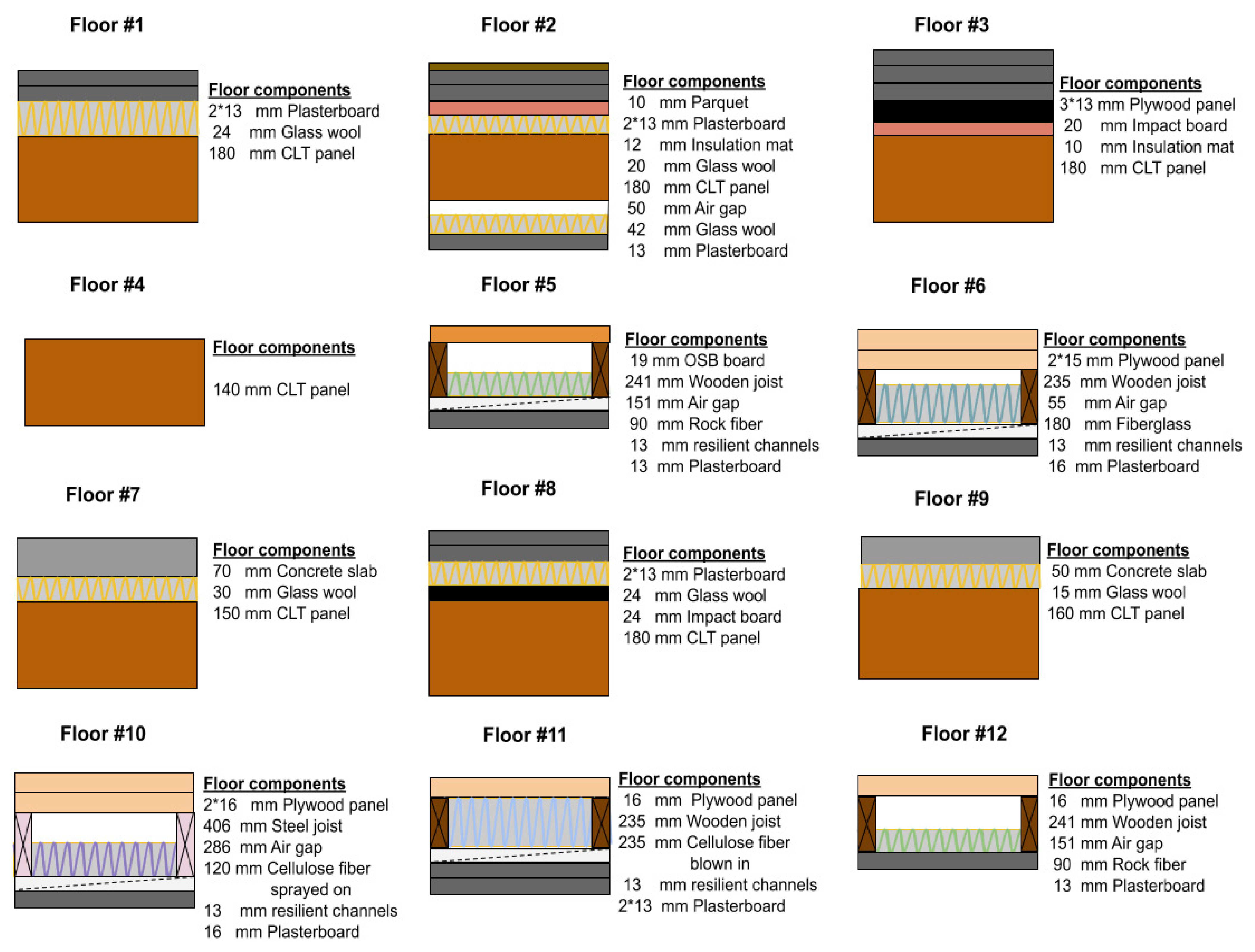
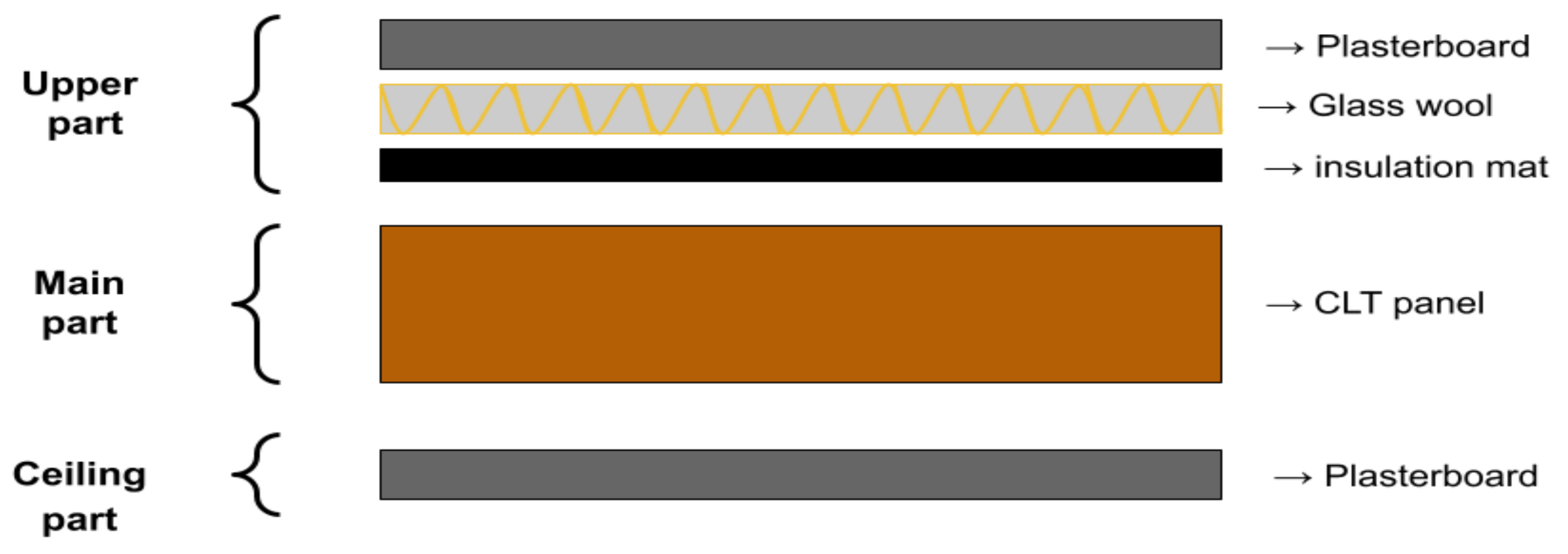
Structure Samples
2.3. Prediction Model Configuration
3. Results and Discussion
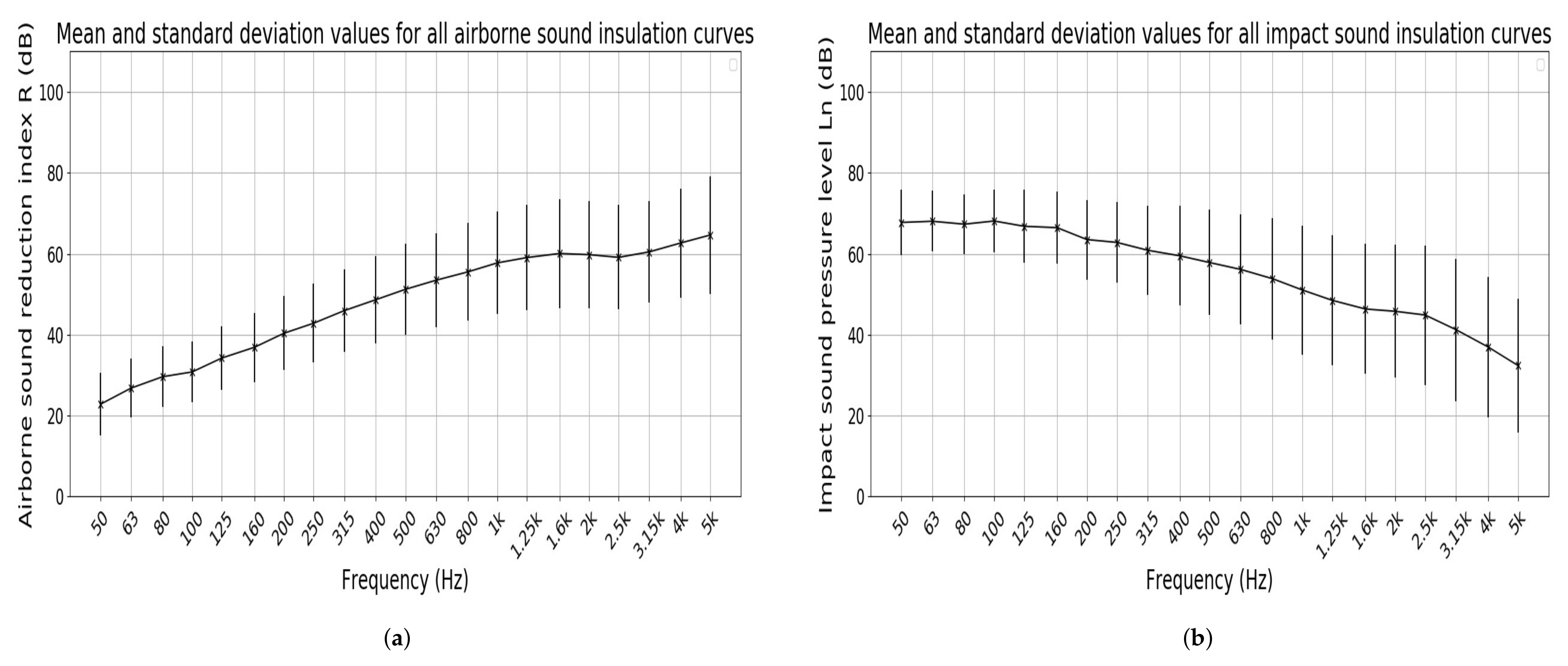
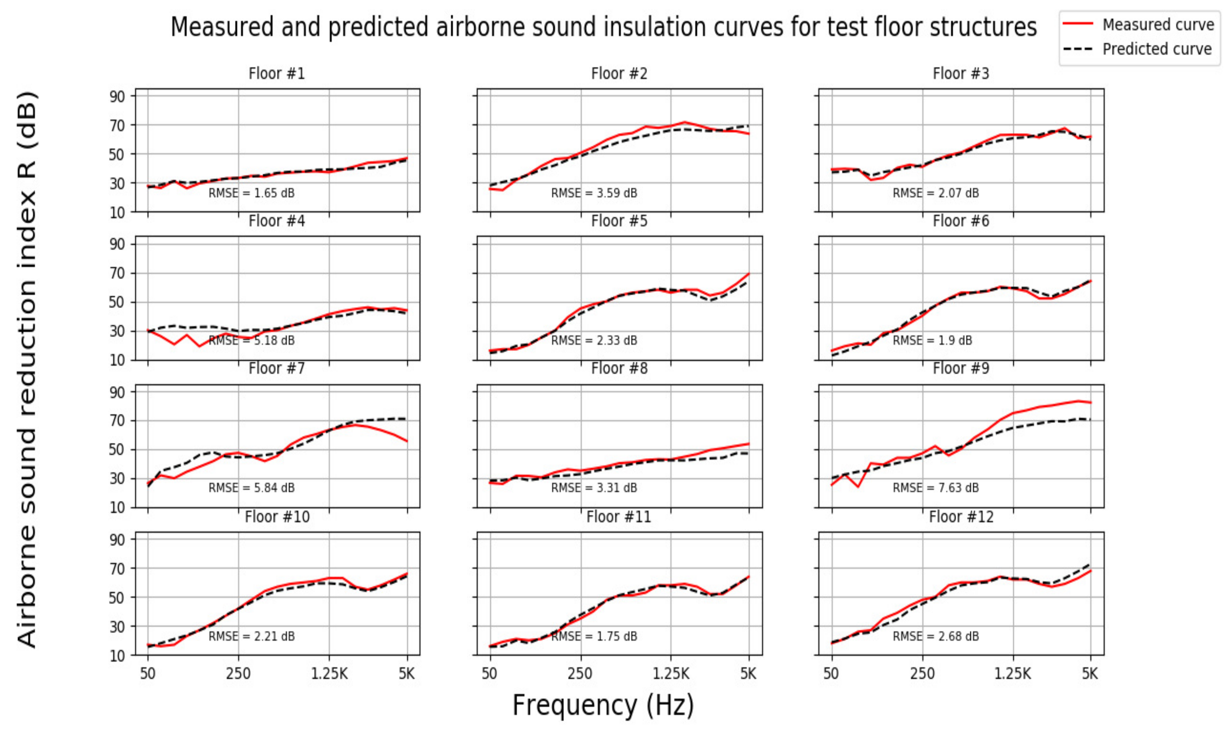
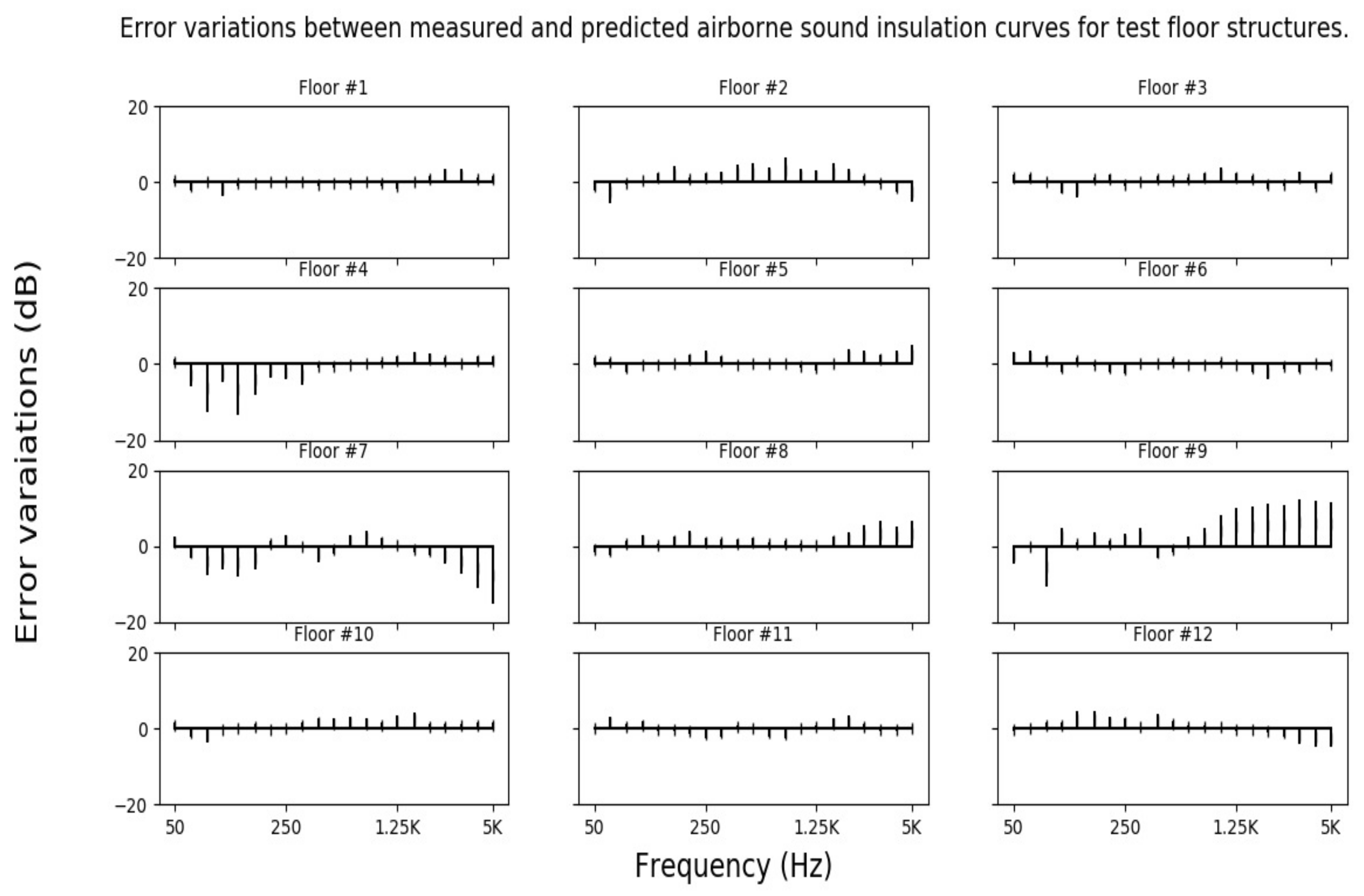
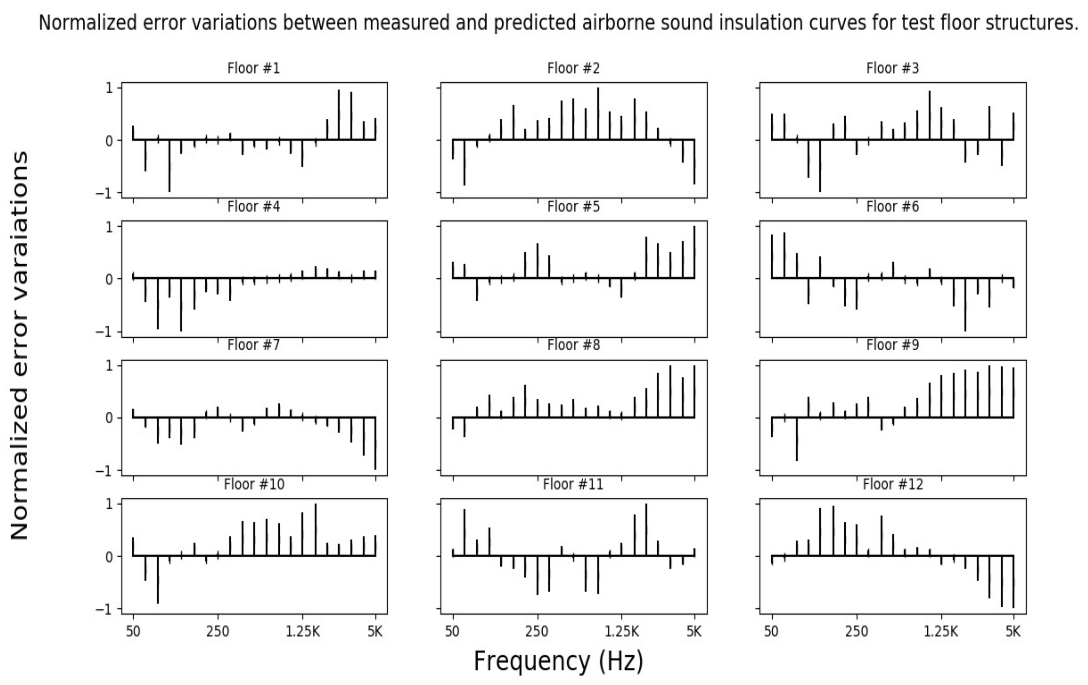
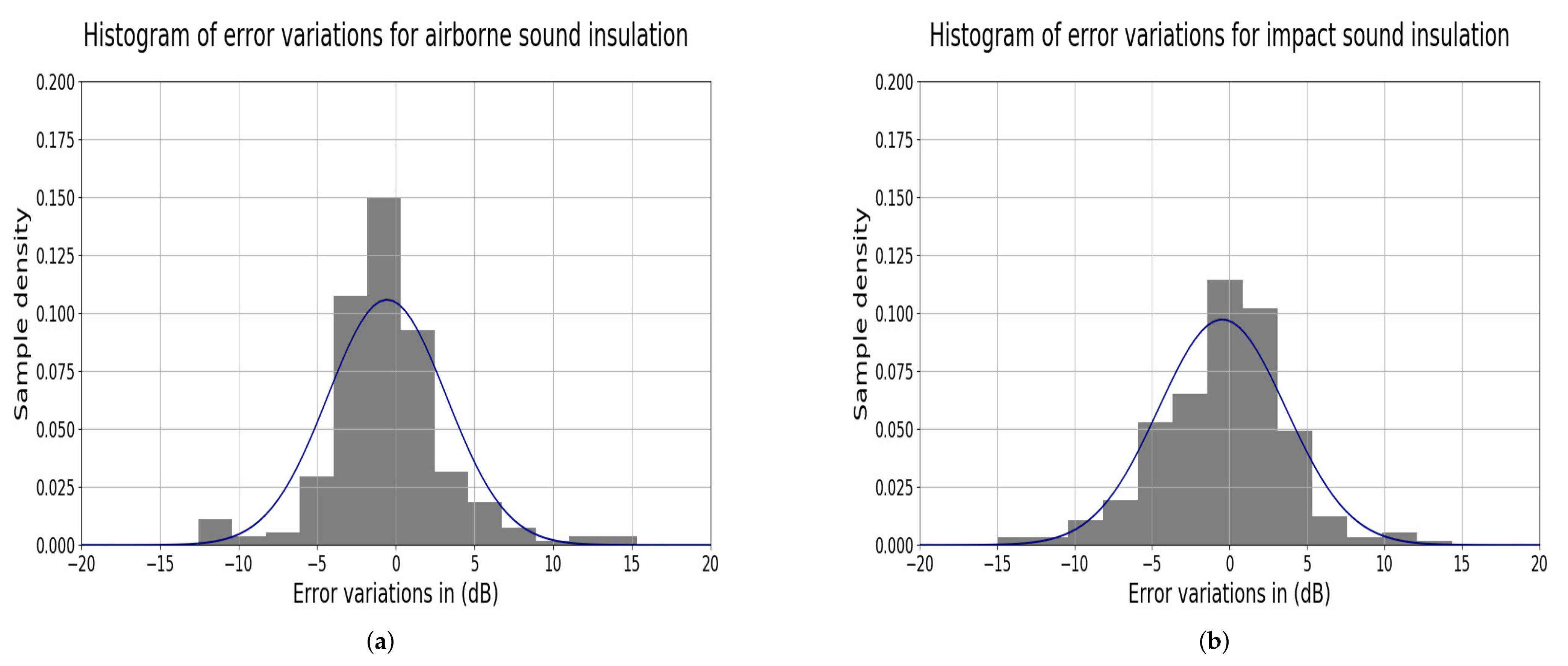
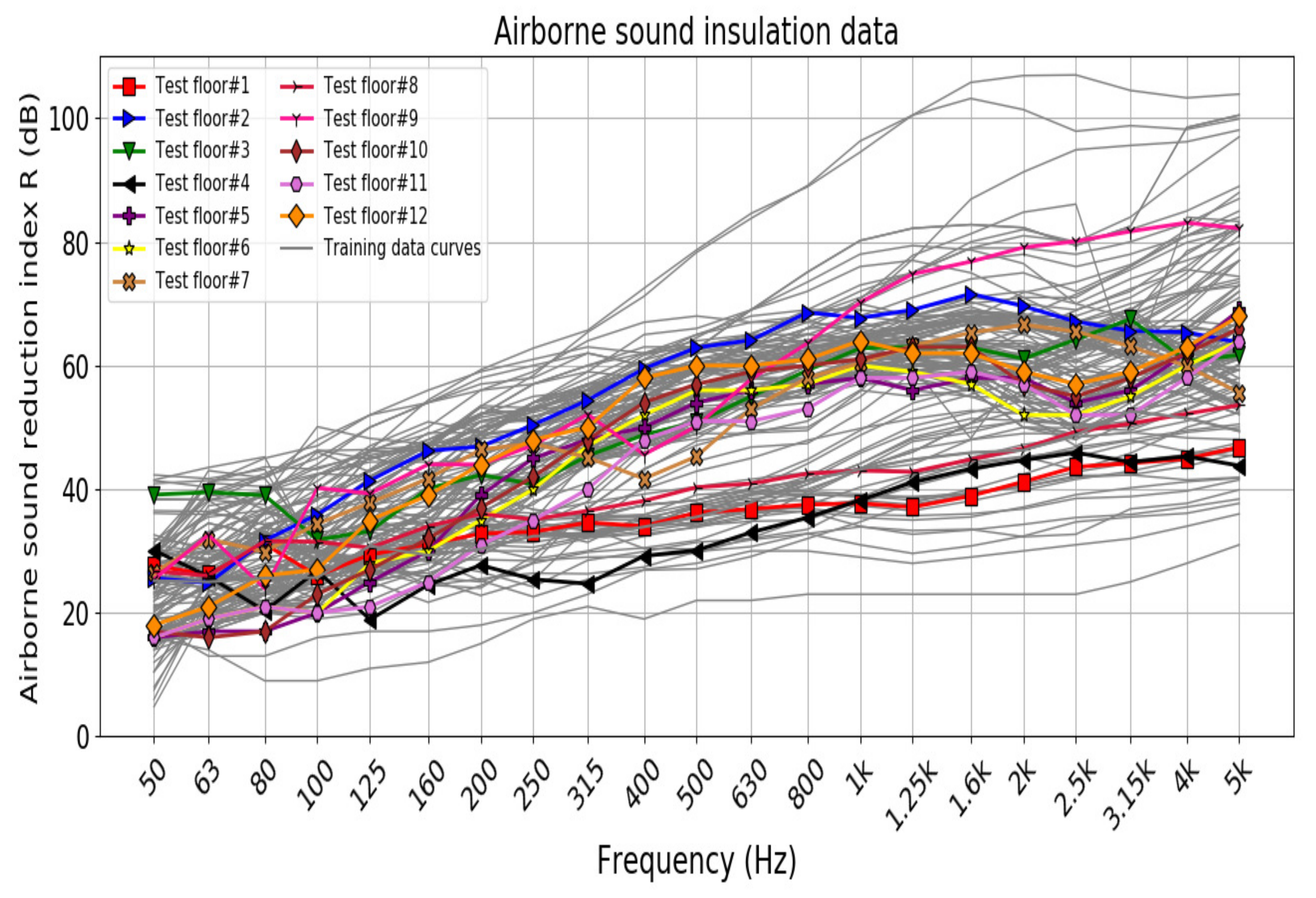
3.1. Prediction of Airborne Sound Insulation
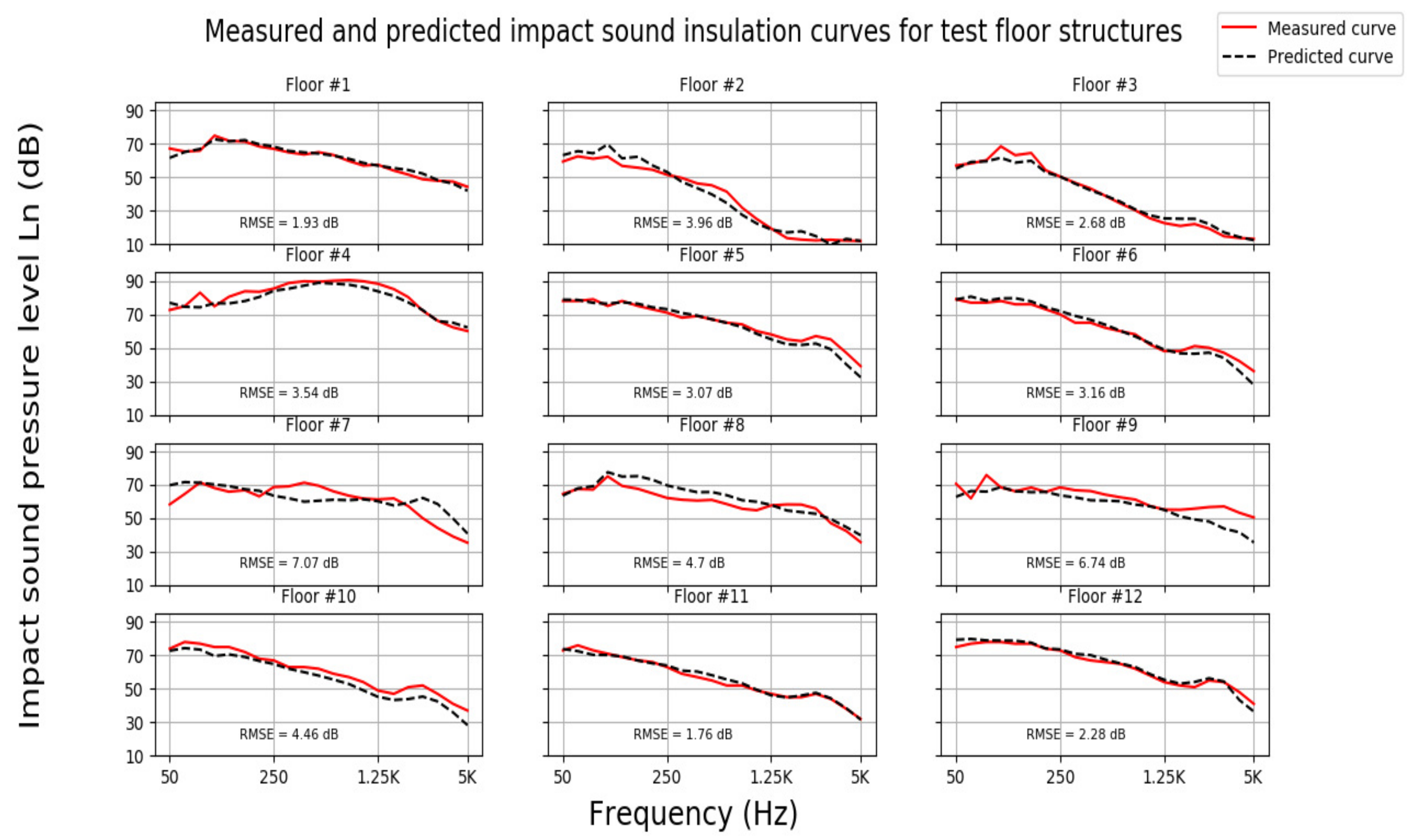
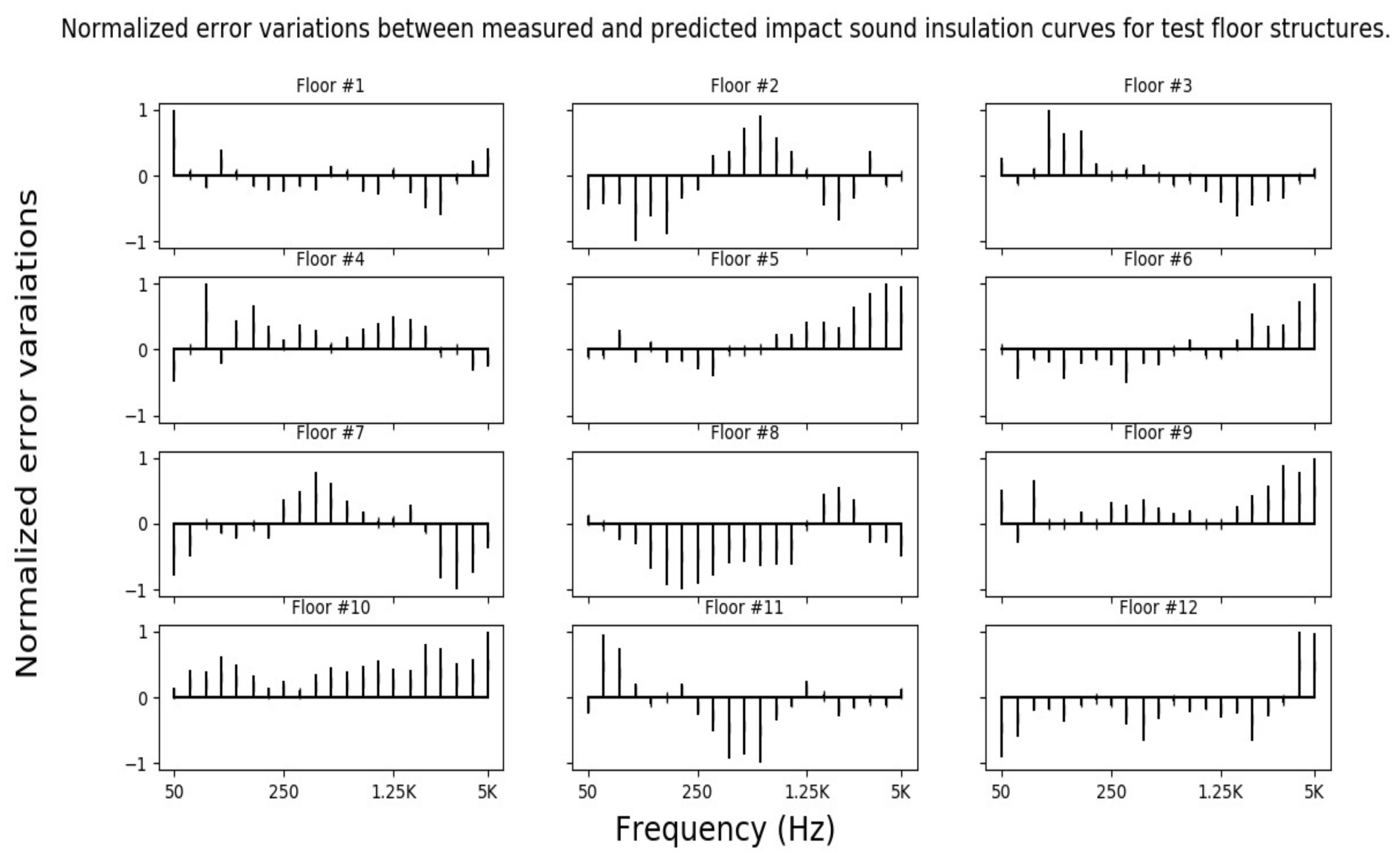
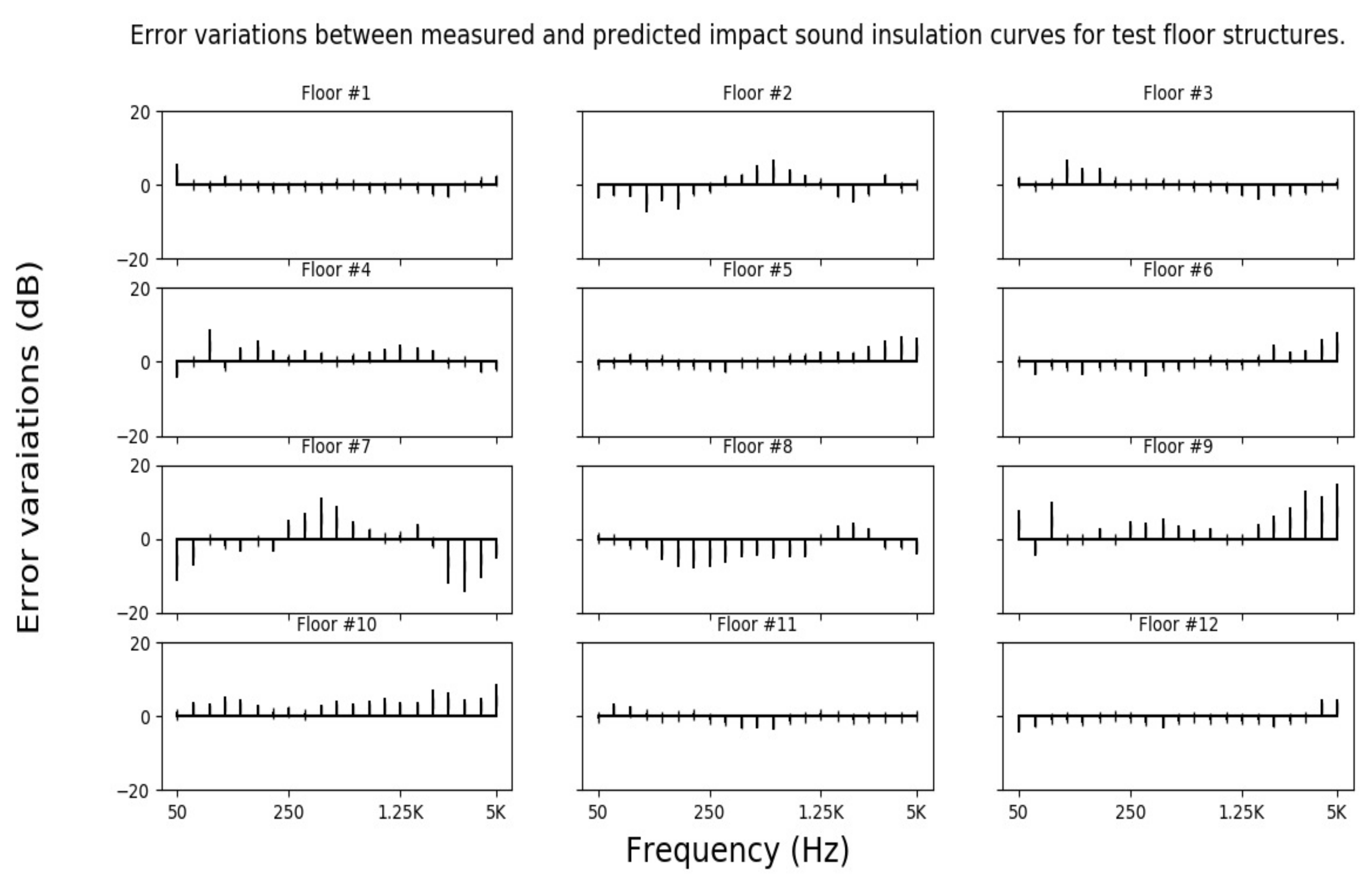
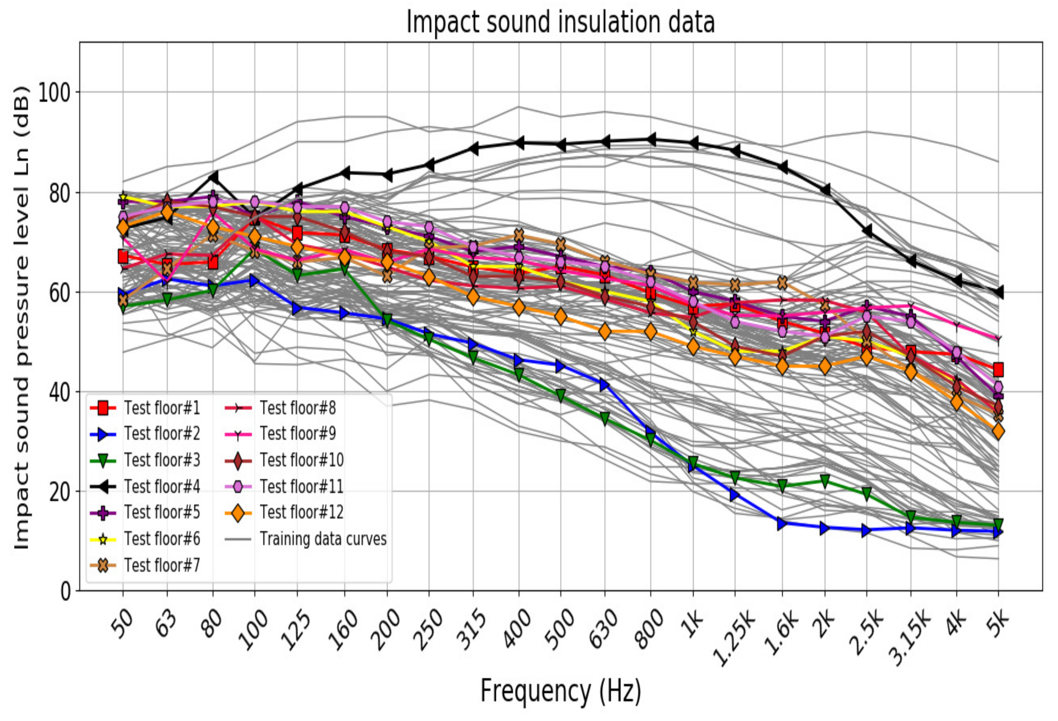
3.2. Prediction of Impact Sound Insulation
3.3. Sensitivity Analysis
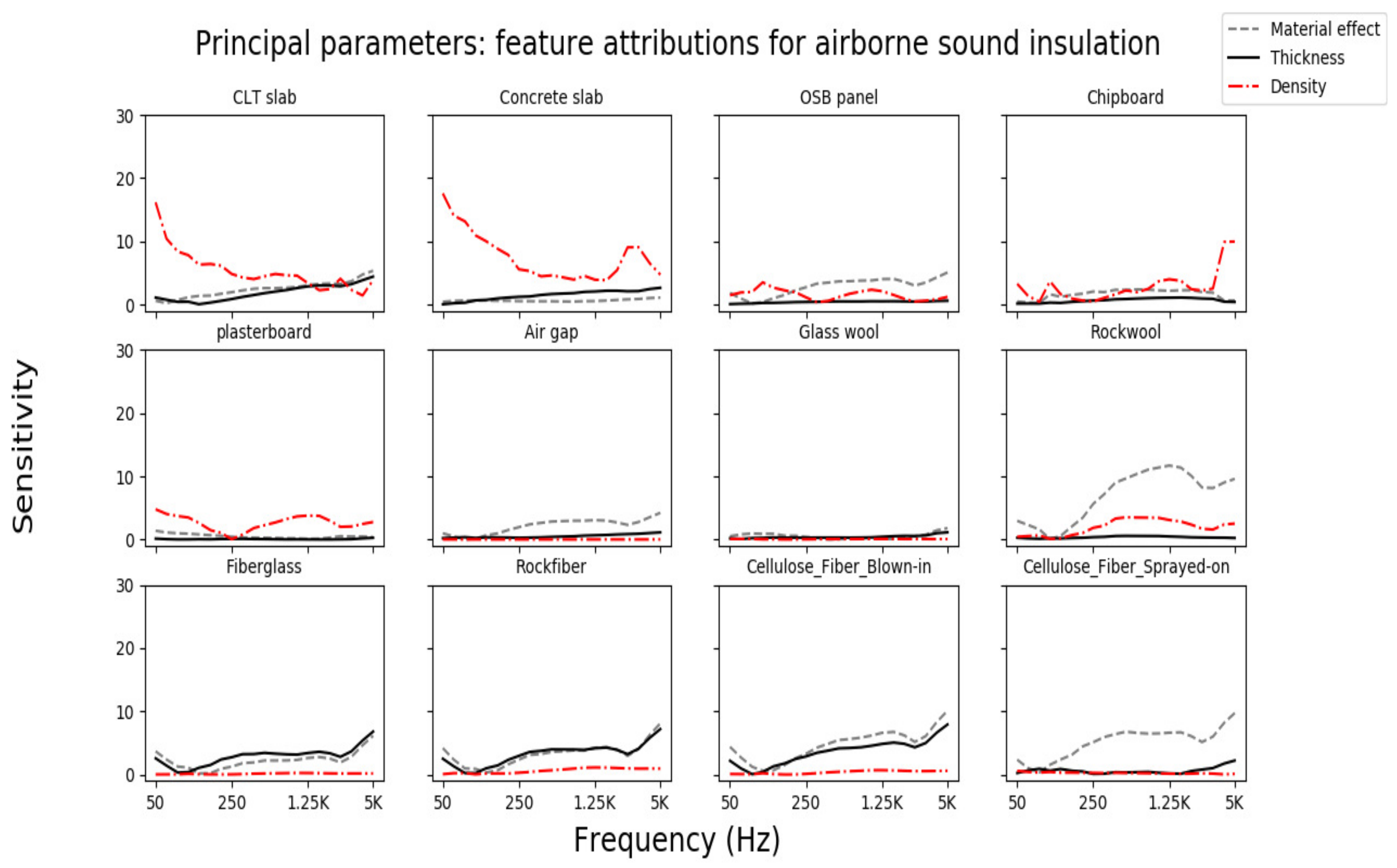
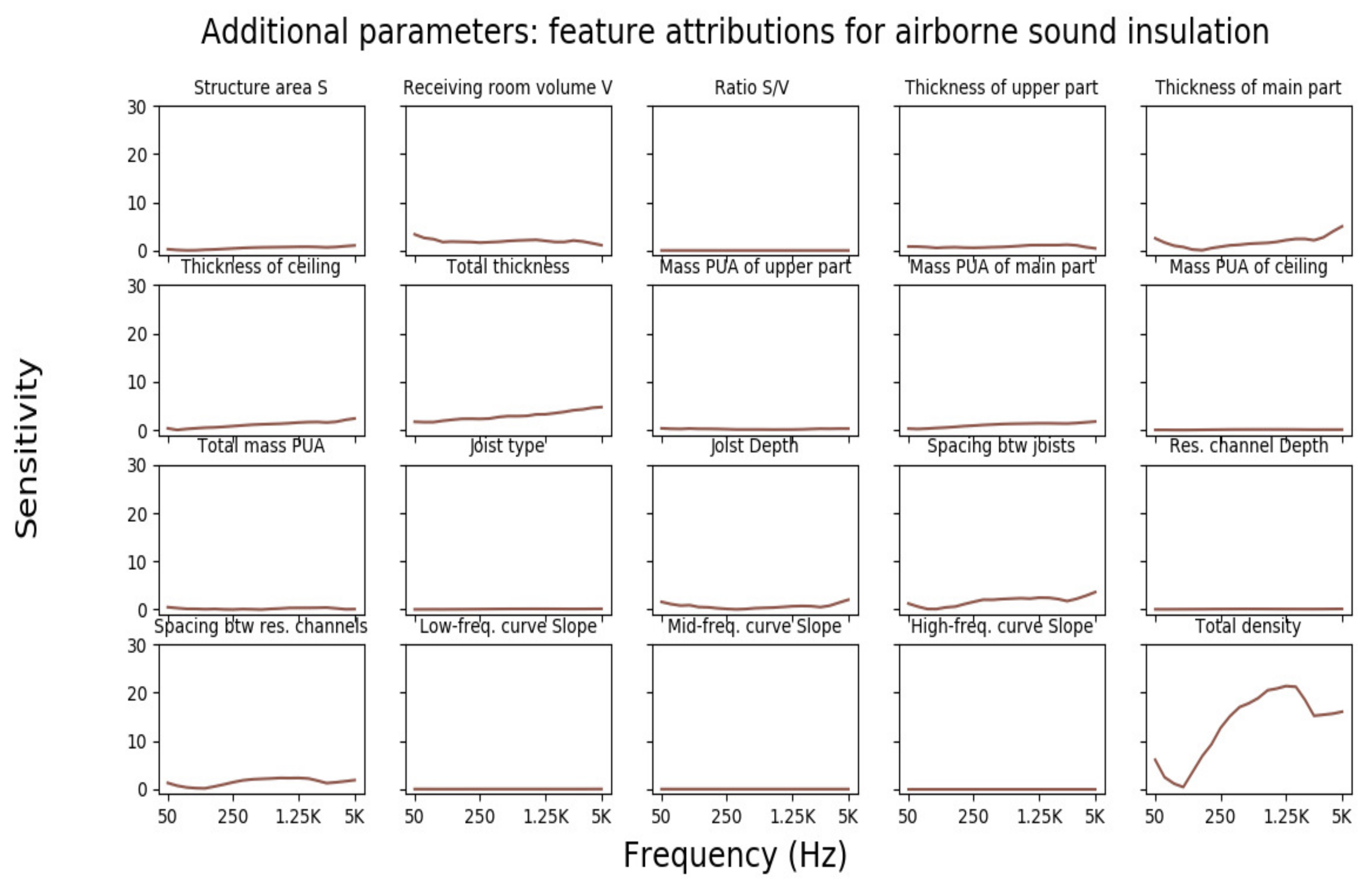
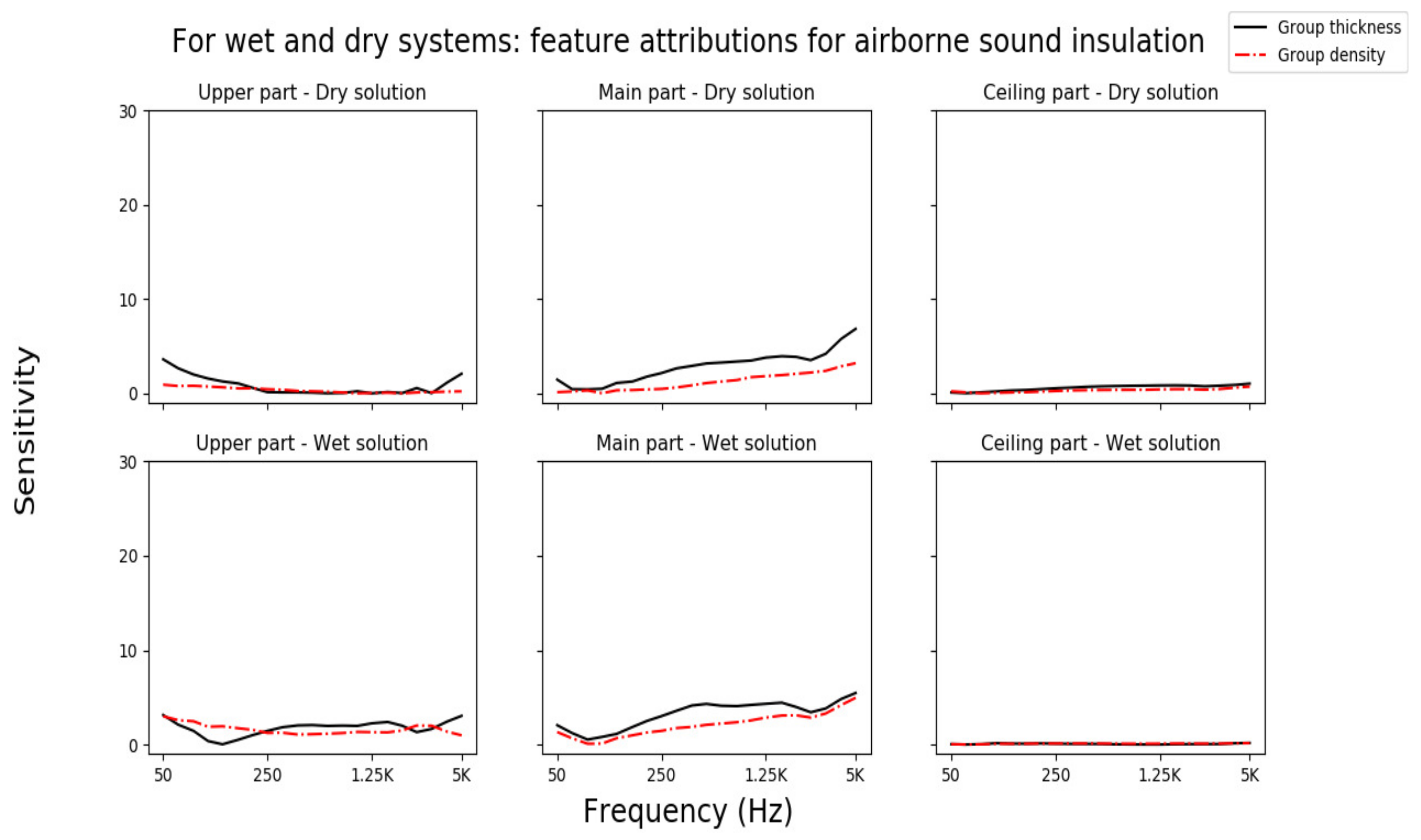
3.3.1. Feature Attributions for Airborne Sound Insulation
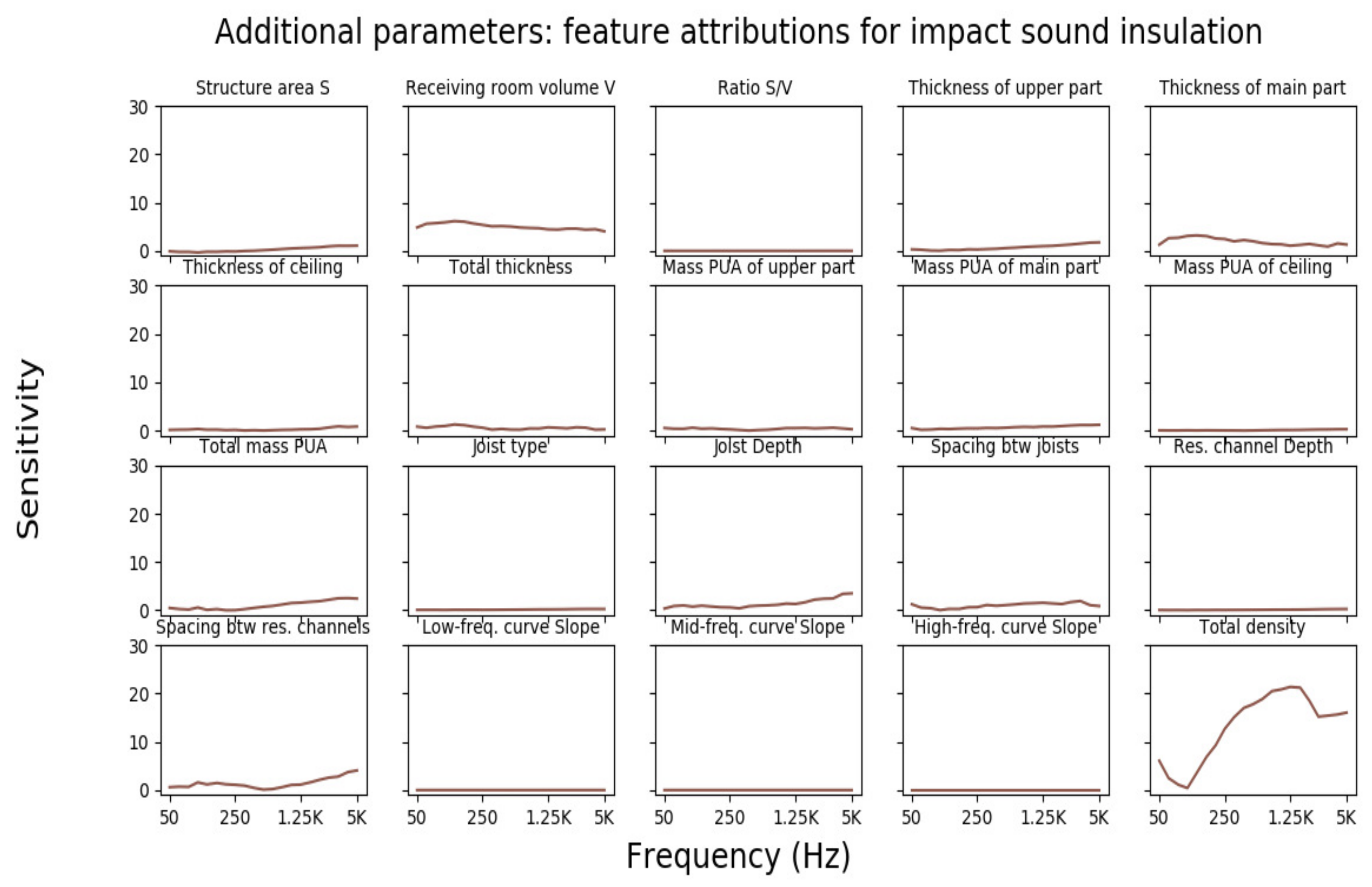
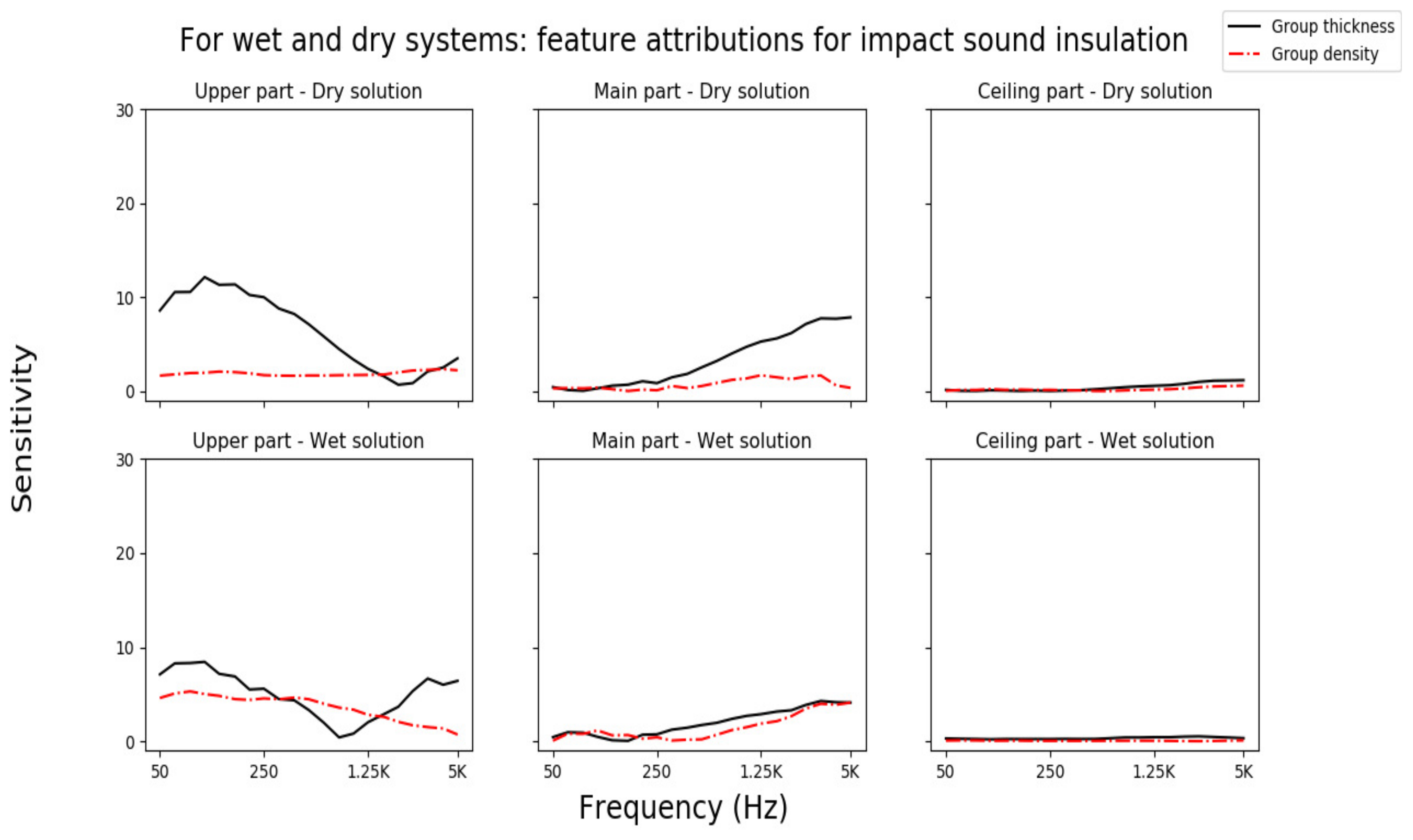
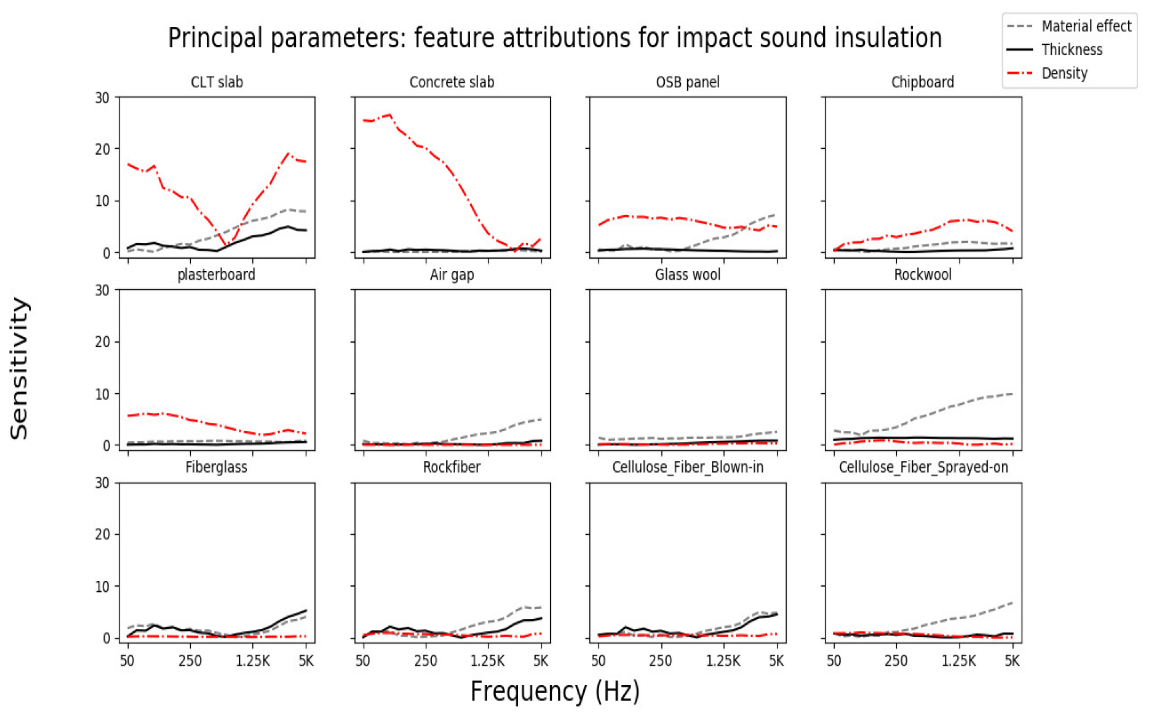
3.3.2. Feature Attributions for Impact Sound Insulation
3.3.3. Common Observations for Airborne and Impact Sound Prediction
4. Conclusions
Author Contributions
Funding
Institutional Review Board Statement
Informed Consent Statement
Data Availability Statement
Acknowledgments
Conflicts of Interest
Appendix A


References
- Hassan, O.A. Building Acoustics and Vibration: Theory and Practice; World Scientific Publishing Company: Singapore, 2009. [Google Scholar]
- Vardaxis, N.G.; Bard, D.; Persson Waye, K. Review of acoustic comfort evaluation in dwellings—part I: Associations of acoustic field data to subjective responses from building surveys. Build. Acoust. 2018, 25, 151–170. [Google Scholar] [CrossRef] [Green Version]
- ISO.140-03; Acoustics–Measurement of Sound Insulation in Buildings and of Building Elements—Part 3: Laboratory Measurements of Airborne Sound Insulation of Building Elements. International Organization for Standardization: Geneva, Switzerland, 1995.
- ISO.140-06; Acoustics–Measurement of Sound Insulation in Buildings and of Building Elements—Part 6: Laboratory Measurements of Impact Sound Insulation of Floors. International Organization for Standardization: Geneva, Switzerland, 1998.
- ISO.140-2; Acoustics–Laboratory Measurement of Sound Insulation of Building Elements—Part 2: Measurement of Airborne Sound Insulation. International Organization for Standardization: Geneva, Switzerland, 2010.
- ISO.16283-1; Acoustics–Field Measurement of Sound Insulation in Buildings and of Building Elements–Part 1: Airborne Sound Insulation. International Organization for Standardization: Geneva, Switzerland, 2014.
- ISO.140-3; Acoustics–Laboratory Measurement of Sound Insulation of Building Elements—Part 3: Measurement of Impact Sound Insulation. International Organization for Standardization: Geneva, Switzerland, 2010.
- ISO.16283-2; Acoustics–Field Measurement of Sound Insulation in Buildings and of Building Elements—Part 1: Impact Sound Insulation. International Organization for Standardization: Geneva, Switzerland, 2015.
- Vigran, T.E. Building Acoustics; CRC Press: Boca Raton, FL, USA, 2014. [Google Scholar]
- Beranek, L.L.; Work, G.A. Sound transmission through multiple structures containing flexible blankets. J. Acoust. Soc. Am. 1949, 21, 419–428. [Google Scholar] [CrossRef]
- Mulholland, K.; Price, A.; Parbrook, H. Transmission loss of multiple panels in a random incidence field. J. Acoust. Soc. Am. 1968, 43, 1432–1435. [Google Scholar] [CrossRef]
- Kang, H.J.; Ih, J.G.; Kim, J.S.; Kim, H.S. Prediction of sound transmission loss through multilayered panels by using Gaussian distribution of directional incident energy. J. Acoust. Soc. Am. 2000, 107, 1413–1420. [Google Scholar] [CrossRef] [PubMed]
- Davy, J.L. The improvement of a simple theoretical model for the prediction of the sound insulation of double leaf walls. J. Acoust. Soc. Am. 2010, 127, 841–849. [Google Scholar] [CrossRef] [PubMed] [Green Version]
- Van den Wyngaert, J.C.; Schevenels, M.; Reynders, E.P. Predicting the sound insulation of finite double-leaf walls with a flexible frame. Appl. Acoust. 2018, 141, 93–105. [Google Scholar] [CrossRef]
- Serpilli, F.; Di Nicola, G.; Pierantozzi, M. Airborne sound insulation prediction of masonry walls using artificial neural networks. Build. Acoust. 2021, 28, 391–409. [Google Scholar]
- Garg, N.; Dhruw, S.; Gandhi, L. Prediction of sound insulation of sandwich partition panels by means of artificial neural networks. Arch. Acoust. 2017, 42, 643–651. [Google Scholar] [CrossRef] [Green Version]
- Craik, R.; Smith, R. Sound transmission through double leaf lightweight partitions part I: Airborne sound. Appl. Acoust. 2000, 61, 223–245. [Google Scholar] [CrossRef]
- Hongisto, V. Airborne Sound Insulation of Wall Structures: Measurement and Prediction Methods; Helsinki University of Technology: Espoo, Finland, 2000. [Google Scholar]
- Legault, J.; Atalla, N. Sound transmission through a double panel structure periodically coupled with vibration insulators. J. Sound Vib. 2010, 329, 3082–3100. [Google Scholar] [CrossRef]
- Santoni, A.; Davy, J.L.; Fausti, P.; Bonfiglio, P. A review of the different approaches to predict the sound transmission loss of building partitions. Build. Acoust. 2020, 27, 253–279. [Google Scholar] [CrossRef]
- Guigou-Carter, C.; Villot, M.; Wetta, R. Prediction method adapted to wood frame lightweight constructions. Build. Acoust. 2018, 13, 173–188. [Google Scholar] [CrossRef]
- Buratti, C.; Barelli, L.; Moretti, E. Wooden windows: Sound insulation evaluation by means of artificial neural networks. Appl. Acoust. 2013, 74, 740–745. [Google Scholar] [CrossRef]
- Vardaxis, N.G.; Bard, D. Review of acoustic comfort evaluation in dwellings: Part II—Impact sound data associated with subjective responses in laboratory tests. Build. Acoust. 2018, 25, 171–192. [Google Scholar] [CrossRef]
- Vardaxis, N.G.; Bard, D. Review of acoustic comfort evaluation in dwellings: Part III—Airborne sound data associated with subjective responses in laboratory tests. Build. Acoust. 2018, 25, 289–305. [Google Scholar] [CrossRef]
- Radkau, J. Wood: A History; Polity: Cambridge, UK, 2012. [Google Scholar]
- Popovski, M.; Ni, C. Mid-Rise Wood-Frame Construction Handbook; FPInnovations: Vancouver, BC, Canada, 2015. [Google Scholar]
- Chatti, S. Production of Profiles for Lightweight Structures; BoD–Books on Demand: Norderstedt, Germany, 2006. [Google Scholar]
- Rasmussen, B.; Machimbarrena, M. Building Acoustics throughout Europe Volume 1: Towards a Common Framework in Building Acoustics throughout Europe; DiScript Preimpresion, S.L.: Madrid, Spain, 2014. [Google Scholar]
- Vorländer, M. Building acoustics: From prediction models to auralization. In Proceedings of the ACOUSTICS 2006, Christchurch, New Zealand, 20–22 November 2006. [Google Scholar]
- ISO.12354-1; Building Acoustics–Estimation of Acoustic Performance of Buildings from the Performance of Elements—Part 1: Airborne Sound Insulation between Rooms. International Organization for Standardization: Geneva, Switzerland, 2017.
- ISO.12354-2; Building Acoustics–Estimation of Acoustic Performance of Buildings from the Performance of Elements—Part 2: Impact Sound Insulation between Rooms. International Organization for Standardization: Geneva, Switzerland, 2017.
- Chattopadhyay, A.; Manupriya, P.; Sarkar, A.; Balasubramanian, V.N. Neural network attributions: A causal perspective. In Proceedings of the International Conference on Machine Learning, PMLR, Long Beach, CA, USA, 9–15 June 2019. [Google Scholar]
- Abdel-Hamid, O.; Deng, L.; Yu, D. Exploring convolutional neural network structures and optimization techniques for speech recognition. In Interspeech; Citeseer: Princeton, NJ, USA, 2013. [Google Scholar]
- Thai, L.H.; Hai, T.S.; Thuy, N.T. Image classification using support vector machine and artificial neural network. Int. J. Inf. Technol. Comput. Sci. 2012, 4, 32–38. [Google Scholar] [CrossRef] [Green Version]
- Dangeti, P. Statistics for Machine Learning; Packt Publishing Ltd.: Birmingham, UK, 2014. [Google Scholar]
- Mohamed, A.R.; Dahl, G.E.; Hinton, G. Acoustic modeling using deep belief networks. IEEE Trans. Audio Speech Lang. Process. 2011, 20, 14–22. [Google Scholar] [CrossRef]
- Di Loreto, S.; Serpilli, F.; Lori, V.; Squartini, S. Sound Quality Evaluation of Kitchen Hoods; Elsevier: Amsterdam, The Netherlands, 2020. [Google Scholar]
- Serpilli, F.; Lori, V.; Di Loreto, S. Speech recognition assessment in Italian pediatric schools using close-set speech tests: A case of study. In INTER-NOISE and NOISE-CON Congress and Conference Proceedings; Institute of Noise Control Engineering: Reston, VA, USA, 2020; Volume 261. [Google Scholar]
- Sak, H.; Senior, A.; Beaufays, F. Long short-term memory based recurrent neural network architectures for large vocabulary speech recognition. arXiv 2014, arXiv:1402.1128. [Google Scholar]
- Nagaya, K.; Li, L. Control of sound noise radiated from a plate using dynamic absorbers under the optimization by neural network. J. Sound Vib. 1997, 208, 289–298. [Google Scholar] [CrossRef]
- Ma, C.; Chen, C.; Liu, Q.; Gao, H.; Li, Q.; Gao, H.; Shen, Y. Sound quality evaluation of the interior noise of pure electric vehicle based on neural network model. IEEE Trans. Ind. Electron. 2017, 64, 9442–9450. [Google Scholar] [CrossRef]
- Wang, Y.; Shen, G.; Xing, Y. A sound quality model for objective synthesis evaluation of vehicle interior noise based on artificial neural network. Mech. Syst. Signal Process. 2014, 45, 255–266. [Google Scholar] [CrossRef]
- Iannace, G.; Trematerra, A.; Ciaburro, G. Case study: Automated recognition of wind farm sound using artificial neural networks. Noise Control. Eng. J. 2020, 68, 157–167. [Google Scholar] [CrossRef]
- Iannace, G.; Ciaburro, G.; Trematerra, A. Using neural networks to detect wind turbine functioning conditions. Int. J. Autom. Smart Technol. 2020, 10, 145–152. [Google Scholar]
- Ciaburro, G.; Iannace, G.; Passaro, J.; Bifulco, A.; Marano, D.; Guida, M.; Marulo, F.; Branda, F. Artificial neural network-based models for predicting the sound absorption coefficient of electrospun poly (vinyl pyrrolidone)/silica composite. Appl. Acoust. 2020, 169, 107472. [Google Scholar] [CrossRef]
- Iannace, G.; Ciaburro, G.; Trematerra, A. Modelling sound absorption properties of broom fibers using artificial neural networks. Appl. Acoust. 2020, 163, 107239. [Google Scholar] [CrossRef]
- Bader Eddin, M.; Menard, S.; Bard, D.; Kouyoumji, J.L.; Vardaxis, N.G. A Sound Insulation Prediction Model for Floor Structures in Wooden Buildings Using Neural Networks Approach. In INTER-NOISE and NOISE-CON Congress and Conference Proceedings; Institute of Noise Control Engineering: Reston, VA, USA, 2021. [Google Scholar]
- Svozil, D.; Kvasnicka, V.; Pospichal, J. Introduction to multi-layer feed-forward neural networks. Chemom. Intell. Lab. Syst. 1997, 39, 43–62. [Google Scholar] [CrossRef]
- Graupe, D. Principles of Artificial Neural Networks; World Scientific: Singapore, 2013. [Google Scholar]
- Goodfelow, I.; Bengio, Y.; Courville, A. Deep Learning (Adaptive Computation and Machine Learning Series); MIT Press: Cambridge, MA, USA, 2016. [Google Scholar]
- Schmidhuber, J. Deep learning. Scholarpedia 2015, 10, 32832. [Google Scholar] [CrossRef] [Green Version]
- Nielsen, M.A. Neural Networks and Deep Learning; Determination Press: San Francisco, CA, USA, 2015. [Google Scholar]
- Sharma, S.; Sharma, S.; Athaiya, A. Activation functions in neural networks. Towards Data Sci. 2017, 6, 310–316. [Google Scholar] [CrossRef]
- Smilkov, D.; Thorat, N.; Kim, B.; Viégas, F.; Wattenberg, M. Smoothgrad: Removing noise by adding noise. arXiv 2017, arXiv:1706.03825. [Google Scholar]
- Baehrens, D.; Schroeter, T.; Harmeling, S.; Kawanabe, M.; Hansen, K.; Müller, K.R. How to explain individual classification decisions. J. Mach. Learn. Res. 2010, 11, 1803–1831. [Google Scholar]
- Shrikumar, A.; Greenside, P.; Shcherbina, A.; Kundaje, A. Not just a black box: Learning important features through propagating activation differences. arXiv 2016, arXiv:1605.01713. [Google Scholar]
- Simonyan, K.; Vedaldi, A.; Zisserman, A. Deep inside convolutional networks: Visualising image classification models and saliency maps. arXiv 2013, arXiv:1312.6034. [Google Scholar]
- Sundararajan, M.; Taly, A.; Yan, Q. Axiomatic attribution for deep networks. In Proceedings of the International Conference on Machine Learning, PMLR, Sydney, Australia, 6–11 August 2017; pp. 3319–3328. [Google Scholar]
- Ruder, S. An overview of gradient descent optimization algorithms. arXiv 2016, arXiv:1609.04747. [Google Scholar]
- Warnock, A. Summary Report for Consortium on Fire Resistance and Sound Insulation of Floors: Sound Transmission and Impact Insulation Data; Institute for Research in Construction, National Research Council Canada: Ottawa, ON, Canada, 2005. [Google Scholar]
- ASTM.E90-09; Standard Test Method for Laboratory Measurement of Airborne Sound Transmission Loss of Building Partitions and Elements. ASTM International: West Conshohocken, PA, USA, 2016.
- ASTM.E492-09; Standard Test Method for Laboratory Measurement of Impact Sound Transmission through Floor-ceiling Assemblies using the Tapping Machine. ASTM International: West Conshohocken, PA, USA, 2016.
- ISO.717-1; Acoustics—Rating of Sound Insulation in Buildings and of Buildings Elements—Part 1: Airborne Sound Insulation. International Organization for Standardization: Geneva, Switzerland, 2013.
- ISO.717-2; Acoustics—Rating of Sound Insulation in Buildings and of Buildings Elements—Part 2: Impact Sound Insulation. International Organization for Standardization: Geneva, Switzerland, 2013.
- Widenius, M.; Axmark, D.; Arno, K. MySQL Reference Manual: Documentation from the Source; O’Reilly Media, Inc.: Newton, MA, USA, 2002. [Google Scholar]
- Géron, A. Hands-On Machine Learning with Scikit-Learn, Keras, and TensorFlow: Concepts, Tools, and Techniques to Build Intelligent Systems; O’Reilly Media, Inc.: Newton, MA, USA, 2019. [Google Scholar]
- Aggarwal, C.C. Neural Networks and Deep Learning; Springer: Berlin/Heidelberg, Germany, 2018; Volume 10. [Google Scholar]
- Mastromichalakis, S. ALReLU: A different approach on Leaky ReLU activation function to improve Neural Networks Performance. arXiv 2020, arXiv:2012.07564. [Google Scholar]
- Xu, J.; Li, Z.; Du, B.; Zhang, M.; Liu, J. Reluplex made more practical: Leaky ReLU. In Proceedings of the 2020 IEEE Symposium on Computers and Communications (ISCC), Rennes, France, 7–10 July 2020; IEEE: Piscataway, NJ, USA, 2020. [Google Scholar]
- Kingma, D.P.; Ba, J. Adam: A method for stochastic optimization. arXiv 2014, arXiv:1412.6980. [Google Scholar]
- Tato, A.; Nkambou, R. Improving Adam Optimizer. 2018. Available online: https://openreview.net/forum?id=HJfpZq1DM (accessed on 9 November 2021).
- Rindel, J.H. Sound Insulation in Buildings; CRC Press: Boca Raton, FL, USA, 2017. [Google Scholar]
- Blazier, W.E., Jr.; DuPree, R.B. Investigation of low-frequency footfall noise in wood-frame, multifamily building construction. J. Acoust. Soc. Am. 1994, 96, 1521–1532. [Google Scholar] [CrossRef]
- Sipari, P. Sound insulation of multi-storey houses—A summary of Finnish impact sound insulation results. Build. Acoust. 2000, 7, 15–30. [Google Scholar] [CrossRef]
- Ljunggren, F.; Ågren, A. Potential solutions to improved sound performance of volume based lightweight multi-storey timber buildings. Appl. Acoust. 2011, 72, 231–240. [Google Scholar] [CrossRef]
- Schoenwald, S.; Zeitler, B.; Nightingale, T.R. Influence of receive room properties on impact sound pressure level measured with heavy impact sources. In Proceedings of the Euroregio 2010 Congress on Sound and Vibration, Ljubljana, Slovenia, 15–18 September 2010. [Google Scholar]
- Reynders, E.P.; Wang, P.; Lombaert, G. Prediction and uncertainty quantification of structure-borne sound radiation into a diffuse field. J. Sound Vib. 2019, 463, 114984. [Google Scholar] [CrossRef]
- Uris, A.; Llopis, A.; Llinares, J. Effect of the rockwool bulk density on the airborne sound insulation of lightweight double walls. Appl. Acoust. 1999, 58, 327–331. [Google Scholar] [CrossRef]
- Fora-Moncada, A.; Gibbs, B. Prediction of sound insulation at low frequencies using artificial neural networks. Build. Acoust. 2002, 9, 49–71. [Google Scholar] [CrossRef]
- Prato, A.; Schiavi, A.; Ruatta, A. A modal approach for impact sound insulation measurement at low frequency. Build. Acoust. 2016, 23, 110–119. [Google Scholar] [CrossRef]
- Hopkins, C. Sound Insulation; Routledge: London, UK, 2012. [Google Scholar]
- Graf, R.F. Modern Dictionary of Electronics; Newnes: London, UK, 1999. [Google Scholar]


| Database | ANN Model | |||||||||
|---|---|---|---|---|---|---|---|---|---|---|
| Number of | ||||||||||
| measurements | 252 | 252 | ||||||||
| airborne | impact | training set | validation set | testing set | ||||||
| 133 | 119 | 204 | 24 | 24 |
| Parameters Used in the Prediction Model | Units | Classes |
|---|---|---|
| − Material types | — | i.e., concrete layer, CLT panel, insulation materials, etc. |
| − Material installation order | — | first/second/etc. |
| − Material thickness | mm | — |
| − Group thickness | mm | upper, main and ceiling parts |
| − Total thickness of the floor | mm | — |
| − Material density | kg/m | — |
| − Group density | kg/m | upper, main and ceiling parts |
| − Total density of the floor | kg/m | — |
| − Area of the floor structure S | m | — |
| − Volume of the receiving room V | m | — |
| − Ratio | — | — |
| − Group mass P.U.A | kg/m | upper, main and ceiling parts |
| − Total mass P.U.A | kg/m | — |
| − Joist type | — | metal/wooden |
| − Joist depth | mm | — |
| − Spacing between joists | mm | — |
| − Resilient channel depth | mm | — |
| − Spacing between resilient channels | mm | — |
| − Curve slope | — | low (50–200 Hz), middle (250–1000 Hz), high frequencies (1250–5000 Hz) |
| Floor No. | (dB) | (dB) | (dB) | ||||
|---|---|---|---|---|---|---|---|
| 1 | 1.65 | 38 | 0 | 1 | 39 | −1 | 0 |
| 2 | 3.59 | 61 | −2 | −4 | 59 | −2 | −2 |
| 3 | 2.07 | 54 | −2 | −1 | 54 | E2 | −1 |
| 4 | 5.18 | 35 | 0 | 0 | 37 | −1 | 0 |
| 5 | 2.33 | 49 | −4 | −5 | 49 | −4 | −5 |
| 6 | 1.9 | 48 | −3 | −3 | 50 | −4 | −5 |
| 7 | 5.84 | 54 | −2 | −2 | 54 | −1 | 0 |
| 8 | 3.31 | 43 | 0 | 0 | 41 | −1 | 0 |
| 9 | 7.63 | 57 | −1 | −3 | 56 | −2 | −1 |
| 10 | 2.21 | 50 | −3 | −5 | 51 | −4 | −5 |
| 11 | 1.75 | 44 | −2 | 46 | −4 | −4 | |
| 12 | 2.68 | 55 | −3 | −4 | 54 | −4 | −5 |
| Floor No. | (dB) | (dB) | (dB) | ||||
|---|---|---|---|---|---|---|---|
| 1 | 1.93 | 64 | 1 | 1 | 64 | 0 | 0 |
| 2 | 3.96 | 48 | 2 | 6 | 53 | 4 | 6 |
| 3 | 2.68 | 53 | 3 | 4 | 48 | 2 | 4 |
| 4 | 3.54 | 88 | −4 | −4 | 85 | −4 | −4 |
| 5 | 3.07 | 68 | 0 | 3 | 67 | 1 | 4 |
| 6 | 3.16 | 66 | 1 | 4 | 68 | 2 | 4 |
| 7 | 7.07 | 64 | −2 | −1 | 66 | −5 | −2 |
| 8 | 4.7 | 64 | −1 | 0 | 66 | 1 | 1 |
| 9 | 6.74 | 64 | −2 | 1 | 60 | 0 | 1 |
| 10 | 4.46 | 63 | 1 | 5 | 60 | 1 | 5 |
| 11 | 1.76 | 60 | 1 | 6 | 60 | 0 | 5 |
| 12 | 2.28 | 68 | 0 | 2 | 70 | 0 | 3 |
| Root Mean Square Errors in dB | |||
|---|---|---|---|
| Frequency Range | Low | Middle | High |
| 50–200 Hz | 250–1000 Hz | 1250–5000 Hz | |
| R (airborne sound) | 3.76 | 2.55 | 4.79 |
| (impact sound) | 3.79 | 3.48 | 4.97 |
Publisher’s Note: MDPI stays neutral with regard to jurisdictional claims in published maps and institutional affiliations. |
© 2022 by the authors. Licensee MDPI, Basel, Switzerland. This article is an open access article distributed under the terms and conditions of the Creative Commons Attribution (CC BY) license (https://creativecommons.org/licenses/by/4.0/).
Share and Cite
Bader Eddin, M.; Ménard, S.; Bard Hagberg, D.; Kouyoumji, J.-L.; Vardaxis, N.-G. Prediction of Sound Insulation Using Artificial Neural Networks—Part I: Lightweight Wooden Floor Structures. Acoustics 2022, 4, 203-226. https://doi.org/10.3390/acoustics4010013
Bader Eddin M, Ménard S, Bard Hagberg D, Kouyoumji J-L, Vardaxis N-G. Prediction of Sound Insulation Using Artificial Neural Networks—Part I: Lightweight Wooden Floor Structures. Acoustics. 2022; 4(1):203-226. https://doi.org/10.3390/acoustics4010013
Chicago/Turabian StyleBader Eddin, Mohamad, Sylvain Ménard, Delphine Bard Hagberg, Jean-Luc Kouyoumji, and Nikolaos-Georgios Vardaxis. 2022. "Prediction of Sound Insulation Using Artificial Neural Networks—Part I: Lightweight Wooden Floor Structures" Acoustics 4, no. 1: 203-226. https://doi.org/10.3390/acoustics4010013
APA StyleBader Eddin, M., Ménard, S., Bard Hagberg, D., Kouyoumji, J.-L., & Vardaxis, N.-G. (2022). Prediction of Sound Insulation Using Artificial Neural Networks—Part I: Lightweight Wooden Floor Structures. Acoustics, 4(1), 203-226. https://doi.org/10.3390/acoustics4010013