Article

Computer Modeling of Barrel-Vaulted Sanctuary Exhibiting Flutter Echo with Comparison to Measurements

1
Mechanical Engineering, SUNY New Paltz, New Paltz, NY 12561, USA
2
Acoustics & Audio Group, University of Edinburgh, Edinburgh lEH8 9DF, UK
*
Author to whom correspondence should be addressed.
Acoustics 2020, 2(1), 87-109; https://doi.org/10.3390/acoustics2010007
Submission received: 31 December 2019 / Revised: 5 February 2020 / Accepted: 7 February 2020 / Published: 17 February 2020
(This article belongs to the Special Issue Indoor Soundscape: Integrating Sound, Experience and Architecture)

Abstract

:
Computer modeling in acoustics allows for the prediction of acoustical defects and the evaluation of potential remediations. In this article, computer modeling is applied to the case of a barrel-vaulted sanctuary whose architectural design and construction led to severe flutter echoes along the main aisle, which was later mitigated through acoustical remediations. State-of-the-art geometrical acoustics and wave-based simulations are carried out to analyze the acoustics of this space, with a particular focus on the flutter echoes along the main aisle, before and after remediations. Multi-resolution wavelet and spectrogram analyses are carried out to isolate and characterize flutter echoes within measurements and computer-simulated room impulse responses. Comparisons of simulated responses to measurements are also made in terms of decay times and curves. Simulated room impulse responses from both geometrical acoustics and wave-based methods show evidence of flutter echoes matching measurements, to varying degrees. Time-frequency analyses isolating flutter echoes demonstrate better matches to measurements from wave-based simulated responses, at the cost of longer simulation times than geometrical acoustics simulations. This case study highlights the importance of computer modeling of acoustics in early design phases of architectural planning of worship spaces.

1. Introduction

Computer modeling has been used in the field of room acoustics to predict and analyze the acoustics of spaces for over fifty years [1,2]. Traditionally, computer modeling in acoustics has been based on geometrical acoustics (GA) [3] with its associated ray-tracing and image-source algorithms [1,4] and its various extensions to include diffraction (for an overview of methods, see [5]). GA simulation methods have reached a point where various mature GA-based commercial softwares are available (e.g., [6,7]). However, the limitations of GA are relatively well-known, in that GA is generally only valid for high frequencies, and its extent of validity into low frequencies depends on the room being modeled and on the relative positions of sources and receivers with respect to any obstructions in the space (i.e., the significance of diffraction effects).
Wave-based methods—such as, e.g., finite-element [8], finite-difference [9,10,11,12], and boundary-element methods [13]—offer another avenue to make use of computers in acoustical modeling [14]. Wave-based methods are, in theory, valid for the entire range of audible frequencies and capture all instances of diffraction, but this comes at the cost of higher compute requirements. For example, computer memory storage requirements in wave-based methods generally scale with the cube of the frequency (in three spatial dimensions), and the number of floating-point calculations required can scale even more severely (e.g., to the fourth power of the frequency). As a consequence of these high compute requirements wave-based methods have seen less use over the years than geometrical approaches. On the other hand, wave-based methods tend to be highly parallelizable, and recent progress in parallel implementations [15,16,17,18,19,20], combined with steady increases in compute power from parallel hardware such as graphics processing units (GPUs), are bringing large-scale wave-based simulations to within reach of consumer hardware [21].
There are a variety of acoustical spaces that have been investigated in the literature using computer modeling, including worship spaces [22,23,24,25,26,27,28,29], performance spaces [30,31,32], multi-purpose spaces [33,34], and outdoor ancient theaters [35,36,37]. Room acoustic computer modeling studies have primarily made use of available geometrical acoustics softwares [38], and relatively few have made use of wave-based methods in low-frequencies [28,29,33,36], mainly due to the aforementioned computational costs. Models of flutter echoes has been of interest for some time [39,40,41] and spaces with flutter echoes have been previously analyzed with ray models [42].
This study aims to make use of GA and wave-based acoustic computer modeling in the study of acoustics of the sanctuary of Christ the King (CTK) Charismatic Episcopal Church of New Paltz, NY. Built in 2009, this church has a barrel-vaulted ceiling over the nave portion of the sanctuary, with the floor of the nave carpeted and covered with rows of upholstered chairs, except for a marble-tiled center aisle along the length of the room. As a result of the design choices that left the barrel-vaulted ceiling centered above a rigid aisle, the room exhibited a strong flutter echo along the center aisle of the room. Acoustical remediations were thus called for to mitigate the strong flutter echo. Remediations were carried out in 2018 in the form of panel absorbers mounted on the ceiling above the aisle; see Figure 1. A previous study by the first author [43] details the measurements undertaken and the acoustical remediation carried out, and its effect on decay times in the room.
The present study aims to model this space using state-of-the-art geometrical (Odeon v15) and wave-based (finite-difference time-domain [44]) computer simulations, and compare the obtained simulation results to measurements taken before and after remediations. The GA and wave-based frameworks are chosen because they are, arguably, the two room acoustic simulation methodologies receiving the most interest from the research community currently. This study builds upon a previous preliminary study [45] wherein GA simulations were carried out, but evidence of flutter echoes (as seen in measurements) were not found in simulation results. The purpose of this study is thus to (a) refine the GA computer model and (b) to see if a more general wave-based simulation is able to better reproduce the fine features of such non-diffuse effects. The simulation results from the GA and wave-based models are compared in terms of objective parameters (T(20),T(30)) and energy decay curves. Additionally, as the aforementioned flutter echoes are not well represented by traditional room acoustic objective metrics (which assume a diffuse field), a multi-resolution wavelet analysis is employed for the comparison of flutter echoes in measurements and computer simulation results, along with spectrogram time-frequency analyses. Evidence of flutter echoes are found in simulated room impulse responses, with the wave-based results showing significant similarities to measurements in multi-resolution analyses. This case study is significant because it comprises one of the few studies comparing both wave-based and geometrical acoustics simulations to measurements. Additionally, this case study highlights the need for computer modeling in early design phases of building construction. The contributions of this paper are thus: (a) comparison of measurements from a non-diffuse space with state-of-the-art GA and wave-based simulations of the space (including before and after acoustical remediations); (b) the use of multi-resolution wavelet analyses for the detection and analysis of flutter echoes; (c) discussion and analysis of strengths and weaknesses of computer modeling methodologies in regards to this unique space.
The outline of the rest of this paper is as follows. Section 2 details the methods of the study, including measurements, computer simulation methodologies, and signal processing and analyses. Section 3 provides an overview of the results and time-frequency signal analyses thereof, and a discussion of those results and their implications. Finally, Conclusions are found in Section 4.

2. Methods

The following section includes discussion of the measurement methodology, the modeling methodology, and the signal processing techniques used.

2.1. Measurements

Room impulse response (RIR) measurements were made before and after the installation of the acoustical panels using a logarithmic sine-sweep IR technique specified in ISO 3382-1 [46]. The room under investigation falls into the category of performance space, therefore ISO 3382-1 was considered appropriate for developing the measurement technique. Of the two different room excitation methods supported by this standard, the integrated impulse response method was used, and the logarithmic sine-sweep was selected as the source sound signal. This was selected because of the improvement of the signal-to-noise ratio and reduction in harmonic distortion which it provides. A comprehensive set of measurements was taken using several different sound source and receiver devices and locations. The following describes only the measurements used for the comparison with modeling presented in this study.

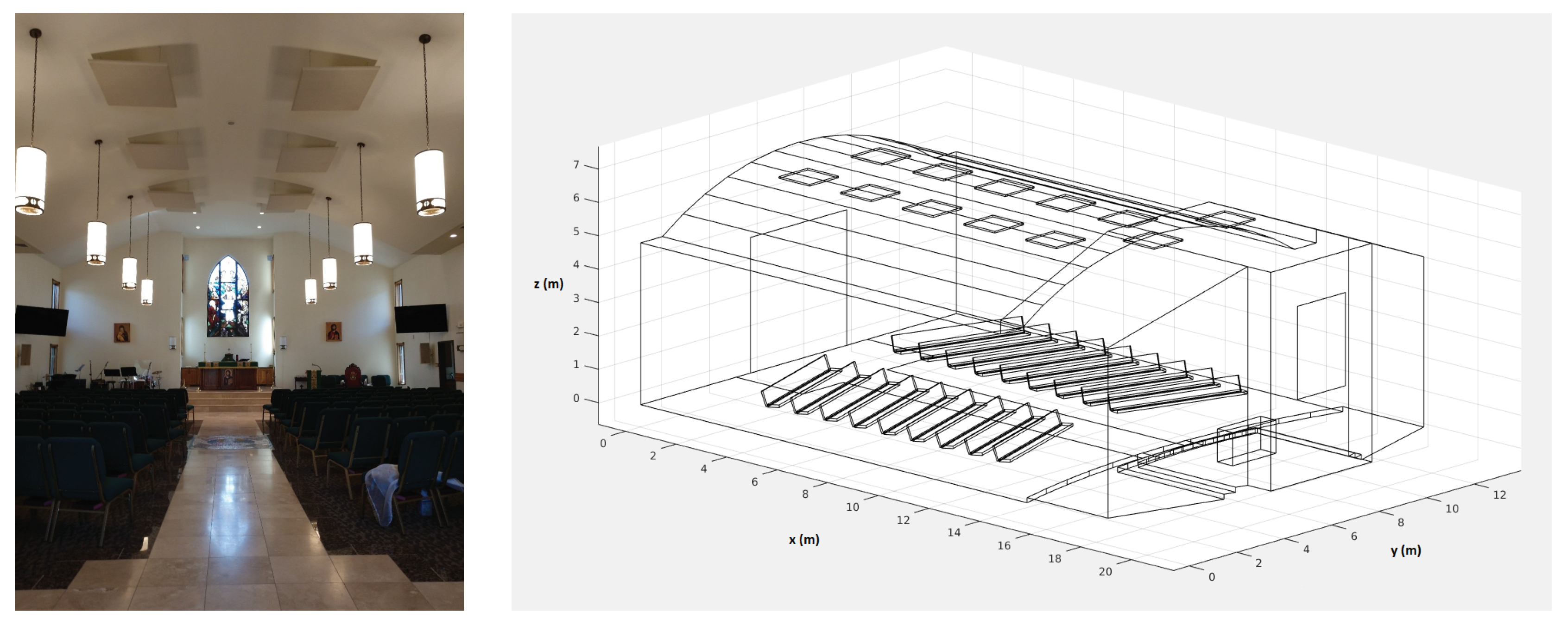
2.1.1. Room Configuration

The room under investigation is a 1546 m 3 sanctuary which contains a barrel-vaulted ceiling over the nave portion of the room. The floor of the nave is completely carpeted and covered with angled rows of upholstered chairs except for a 1.83 m wide marble-tiled center aisle along the length of the room. The barrel-vaulted sanctuary ceiling was constructed with a 10.4 m radius arc with a 11.4 m span and 6.5 m height at the crown. All of the wall surfaces of the sanctuary are built with gypsum board and finished with a standard eggshell paint.
Due to complaints of unintelligibility along the center aisle of the nave, the room configuration underwent acoustical remediation in 2018. This treatment involved the installation of 12 Auralex Acoustics absorbing panels on the ceiling (ten on the barrel vault and two on the flat ceiling above the alter). Each of these panels is 0.05 m × 1.2 m × 1.2 m (2 in × 4 ft × 4 ft). The panels are suspended horizontally from the ceiling, 6 m from the floor, with the center of each panel located 1.5 m from the crown of the barrel-vaulted ceiling.

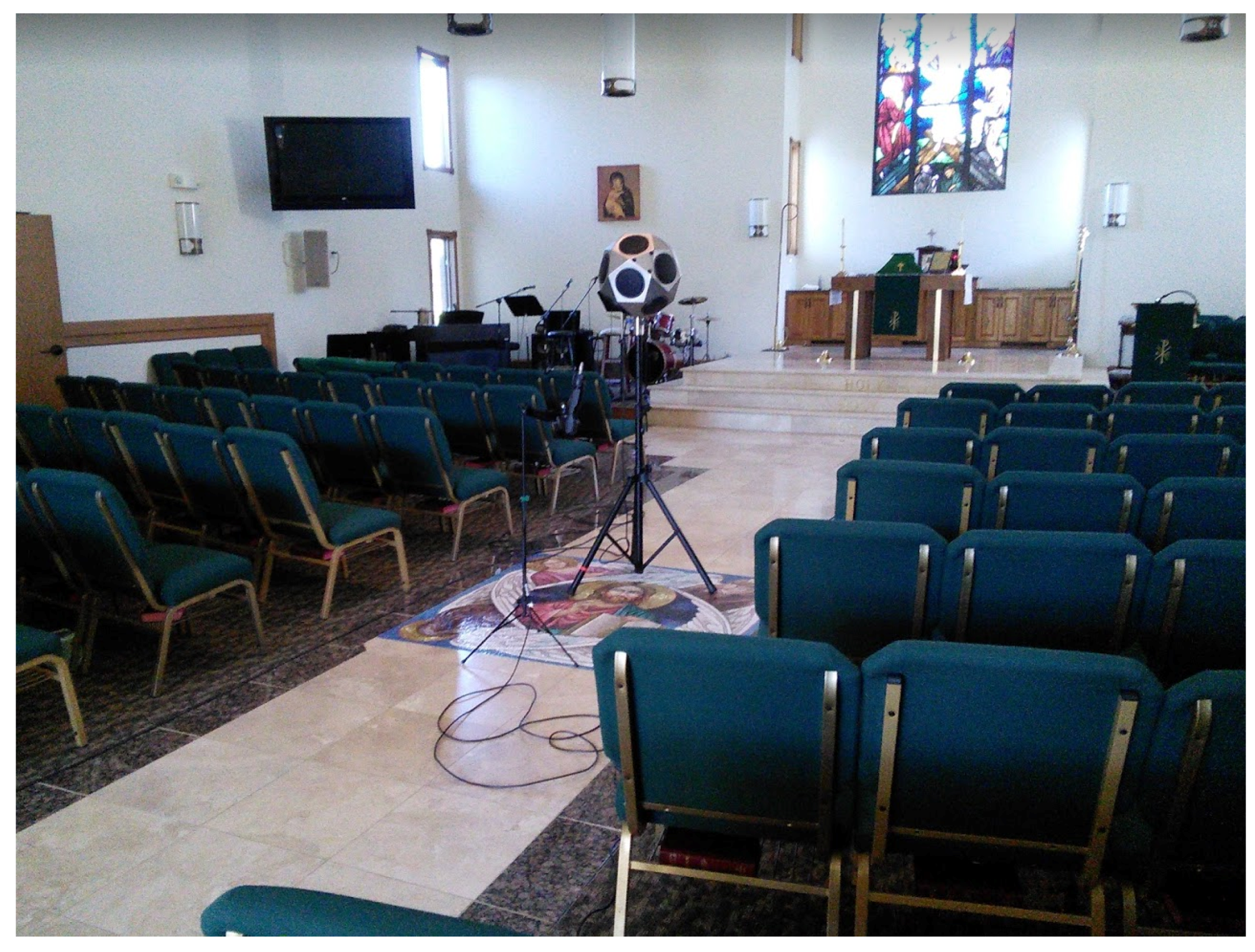
2.1.2. Measurement Equipment

The acoustical measurements used in this comparison were completed by broadcasting a logarithmic sine sweep into the room using a Brüel and Kjær TYPE 4292-L dodecahedral loudspeaker, as shown in Figure 2. The input signal was a 4 s logarithmic sine sweep, with a bandwidth of 44–11,360 Hz chosen to excite the 64 Hz–8 kHz octave bands. Acoustical pressure measurements were collected during the sine sweep using a PCB model 378B20 omni-directional microphone, with a model 426E01 preamp. All data collection was performed at a sampling frequency of 51,200 Hz.

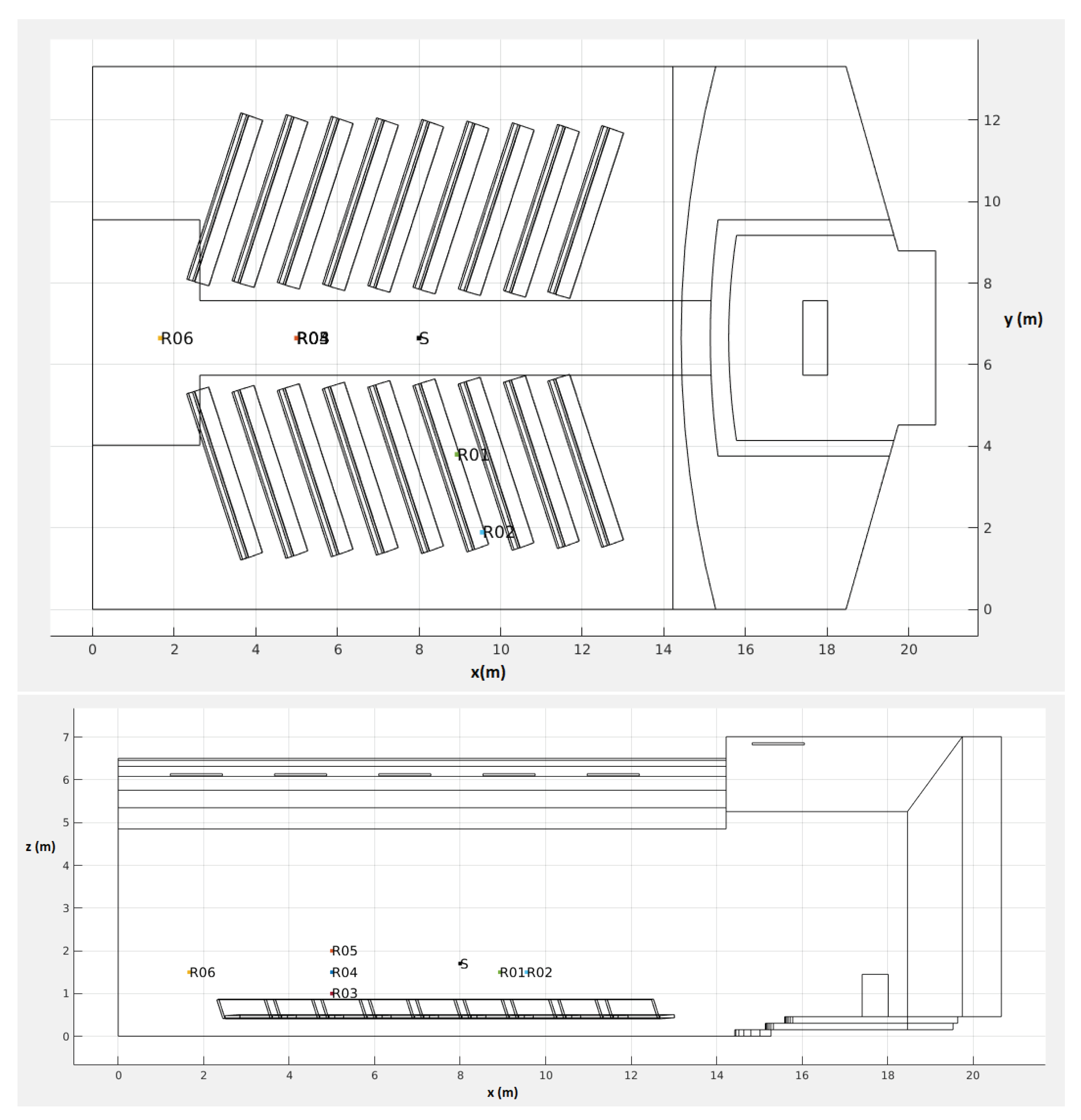
2.1.3. Source and Receiver Locations

Acoustical measurements were taken of both the original configuration and the acoustically treated room. Acoustical data was collected from a wide range of source and receiver locations, corresponding to possible sound source/listener locations during ordinary use of the space.
While a large number of data points were collected in the space, after reviewing the RIRs a small subset of those points which highlight the unique acoustical behavior of the room were strategically selected for comparison with the computer models. All measurements used were taken with the source located in the center of the room along the aisle. This source location was selected for use in the study because it most effectively excited the flutter echo. Additionally, six receiver locations were selected for comparison with the modeling because these locations highlight specific features of the room’s acoustical behavior. This selection included two points located off the aisle, in the audience and four points along the aisle. The location and height of each of the receiver locations are listed on Table 1, and can be seen visually on Figure 3.

2.2. Computer Modeling

In this subsection, a brief overview of the computer modeling techniques (GA and wave-based) is given, along with specific parameters used for the simulations themselves.

2.2.1. Geometrical Acoustics (GA) Methods

Geometrical acoustics assumes that sound travels akin to light rays, i.e., sound travels along rays and these sound rays bounce specularly off objects and/or scatters non-specularly or diffusely [47]. Sound rays can carry amplitude or energy (i.e., magnitude only), and interactions with walls in terms of sound absorption and/or scattering are typically described by frequency-band coefficients taking on values between zero and one [5,48]. Diffraction is not strictly part of the GA framework (by some definitions, GA simply precludes diffraction [49]), but there has been a great deal of work on integrating early edge diffraction into GA simulations, following the idea that diffraction can be described by new sound rays, emanating from edges [50] and applying approximate solutions [49]—or analytic solutions [51] when available. GA is often coupled with statistical models for late decay in the impulse response—i.e., that sound decays evenly throughout the room and can be treated as an ensemble average (i.e., a diffuse field) [52]. For computational reasons in GA simulations, it can be beneficial to take advantage of diffuse-field assumptions to reduce the number of specular rays that are needed to trace a full impulse response, and various popular algorithms have evolved to this effect, such as the “Ray Radiosity Method” employed in Odeon [53] and the “Diffuse Rain” algorithm [54] employed in RAVEN [52]. It would follow, however, that the more reliance there is on scattering and diffuse late-field assumptions, the harder it can be to reproduce any fine features of non-diffuse reverberation (e.g., flutter echoes).

2.2.2. GA Computer Modeling Methodology

The commercial software Odeon, version 15 [53], was used as a tool for GA computer modeling. A computer-aided design (CAD) model of the room was made using Trimble Sketchup, starting from architectural drawings and using refinements from laser measurements in the space (where architectural specifications were not followed exactly in construction). This CAD model of CTK church was built with a compromise between level of detail and suitability for GA modeling; that is, chairs and light fixtures were removed, as these are typically not included in CAD models used for GA simulation, and the curved ceiling was polygonized into twelve flat rectangular sections (see Figure 4). These rectangular sections were marked as “Fractional” surfaces within Odeon, which tells the program to treat each section as one part of a larger curved surface (as recommended [53]). Seats were replaced with two rectangular “audience” surfaces, to which absorption and scattering were applied in order to approximate the seating area (without persons) as best as possible within the chosen GA software framework. Absorption coefficients for each surface material are given in Table 2. Surface-roughness scattering coefficients for each material within Odeon were set to 0.05 (smooth surfaces) from which Odeon estimated octave-band scattering coefficients [53]. These coefficients were chosen based on materials within Odeon’s material database. It should be noted that a detailed calibration campaign was not carried out in this case, as it was understood that such calibrations (e.g., [23]) typically rely on diffuse-field objective parameter measurements, whereas this space was known to be highly non-diffuse, in particular along the aisle where the flutter echo was most pronounced. While there will be unavoidable input data uncertainty in the computer model [55], it was reasoned that a calibration to decay times would not have a significant effect on reproducing the non-diffuse effect of interest here.
In order to obtain a good GA approximation from the Odeon software, 100k rays were used (per receiver) with the transition order of two, where the transition order specifies at which reflection order the software switches from its image-source algorithm to its ray-based algorithm. The number of rays was chosen in order to go beyond the “Precision” recommendations of Odeon, as it was hoped that the ray-based solution would converge to some best solution with a large number of rays. A detailed comparison of results with number of rays used is not within the scope or interest of this study, but it was found that 100k was a good compromise, and significantly more rays did not impact output results. Angle-dependent absorption (ADA) was used for all materials as it was found to have a significant effect on the authenticity of the room impulse response outputs, in particular where one expected to hear flutter echoes. While this choice was made based on perceptual observations, a perceptual similarity experiment was not within the initial scope of this study.

2.2.3. Wave-Based Methods

Wave-based methods aim to solve the wave equation in three spatial dimensions through numerical grids or meshes. The advantage of using a wave-based method is that the numerical solution naturally comprises all wave phenomena, which includes both geometrical behavior and diffraction. However, such numerical solutions can only be resolved in practice up to a given frequency, due to approximation errors and limitations in computational resources. Traditionally, wave-based methods have only been used to resolve modal behavior below the Schroeder frequency [56], but it is becoming increasingly possible to use wave-based methods beyond Schroeder frequencies of rooms thanks to increases in parallel compute power (see, e.g., [20]). In this study, a finite-difference time-domain (FDTD) method was used [10,11,12], which is a regular grid-based method that makes use of some time-marching scheme, in this case Störmer-Verlet integration [57], and finite-difference stencil operations to approximate spatial derivatives in the wave equation in three spatial dimensions [58]. FDTD methods have similarities to simple finite-volume methods [10] and in some cases finite-volume methods can be used as generalizations of FDTD [59] in order to refine numerical boundary conditions to better adapt to non-Cartesian wall-boundaries [60]. The FDTD implementation used in this study follows the finite-volume framework laid out in [60,61,62]. This framework makes use of a frequency-dependent locally-reactive impedance boundary model, which allows for passive realizations of complex impedances [61]. To devise such boundary models, wall absorption data for the wave-based model is also taken from Table 2. However, it should be pointed out that locally-reactive impedances are limited to approximately 0.95 Sabine absorption [47], so numerical clamping was employed for coefficients of acoustical panels whose random-incidence absorption coefficients went beyond the limit of the locally-reactive model.

2.2.4. Wave-Based Computer Modeling Methodology

For the FDTD wave-based model, the Sketchup CAD model of CTK church was modified to include a seating area overtop a carpet surface, since, rather than relying on scattering coefficients to emulate their scattering behavior, the FDTD model can naturally simulate the scattering from seats (see Figure 4). As mentioned above, the FDTD model used followed the framework laid out in [61,62], and a non-Cartesian cubic close-packed (CCP) grid was chosen for efficiency reasons [63], with finite-volume refinements at boundaries. The interior FDTD scheme thus followed the “CCP” scheme featured in [12]. Boundary impedance conditions were set from absorption coefficients given in Table 2, where a passive complex impedance [60] was fit through numerical optimization [44]. The grid spacing for the FDTD model was set such that all frequencies under 8 kHz would have less than 1% numerical dispersion errors, resulting in a grid spacing of approximately 5.5 mm. This FDTD model, with an overarching bounding box of 1950 m 3 and simulating 5 s of impulse response, was run on a cluster of NVIDIA GPUs hosted at the University of Edinburgh, with compute times of approximately one hour per second of impulse response.
The wave-based results, comprising frequencies below 8 kHz, were complemented with high-frequency ray-traced room impulse responses computed using a high-density ray tracing code developed at the University of Edinburgh. As such, the “wave-based” results are in fact “hybrid” wave/ray-based results, but for simplicity the term “wave-based” will be used henceforth, since the majority of the subsequent analyses focus on frequencies below 8 kHz, and in terms of octave bands, 90% of the hybrid RIRs are generated from the wave-based FDTD approach. Nevertheless, it is worth mentioning that for these GA results, 500k rays were traced throughout the scene with specular reflections only (i.e., a strict GA approximation), using angle-dependent absorption (based on a locally-reactive model), and using the same CAD model as for the FDTD simulations. Linear phase, partition-of-unity finite impulse response (FIR) filters were used to combine FDTD and ray-traced outputs.

2.3. Signal Processing of Room Impulse Response

The room impulse response (RIR) of the measured data was calculated for each sine sweep measurement through deconvolution of the recorded signal with the input sine sweep. These RIR waveforms were resampled to both 48 kHz and 45.254 kHz (following [64]), and used as a basis of all additional signal processing procedures as described.
  • Spectrogram Analysis: Spectrograms were generated from 48 kHz sampled RIR data using a 10 ms Hann window with 120 sample overlap.
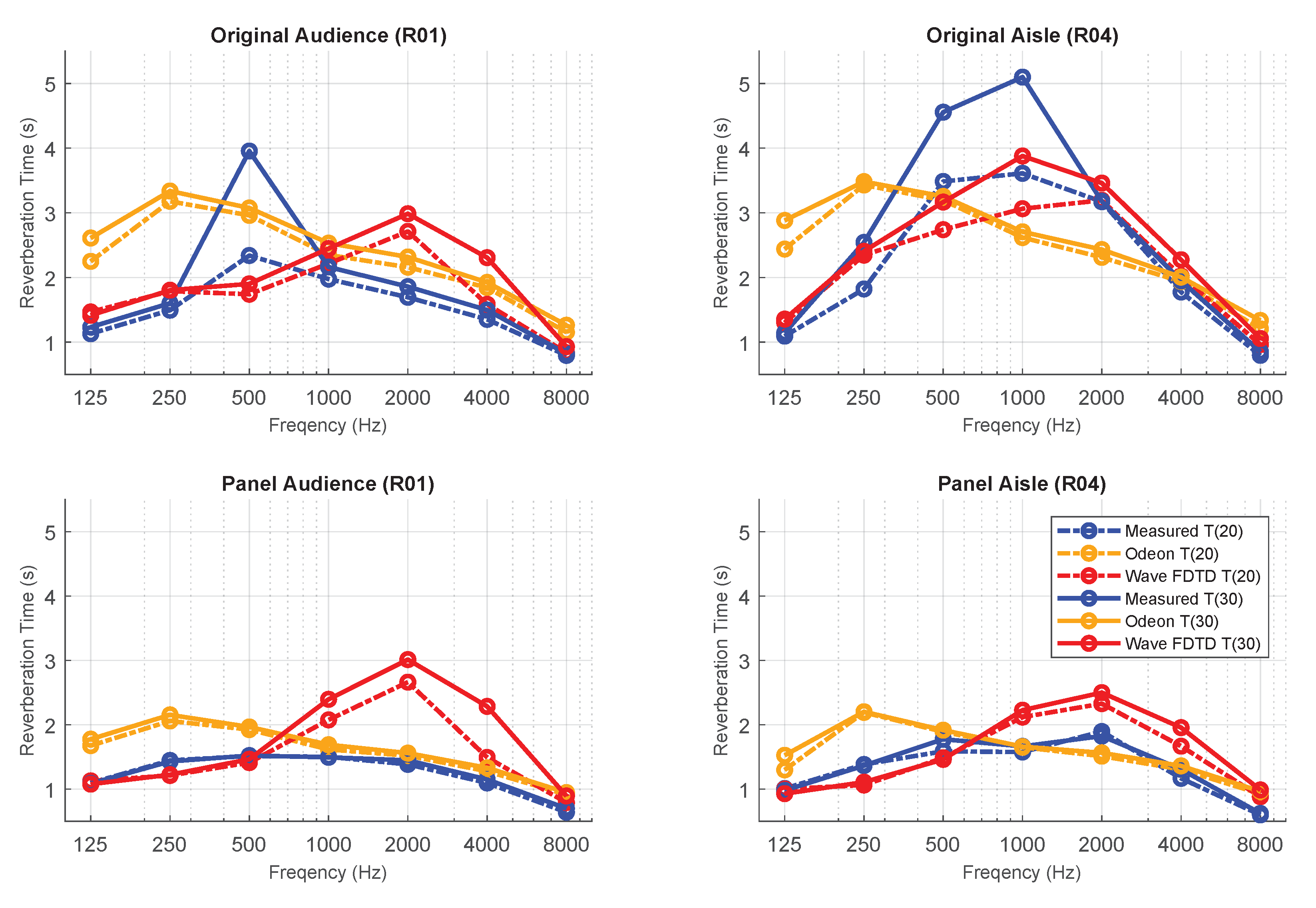
  • Reverberation Time: Reverberation times (T(20) and T(30)) were calculated from the 48 kHz sampled RIR data for the 125–8000 Hz octave bands using the ITA toolbox [65].
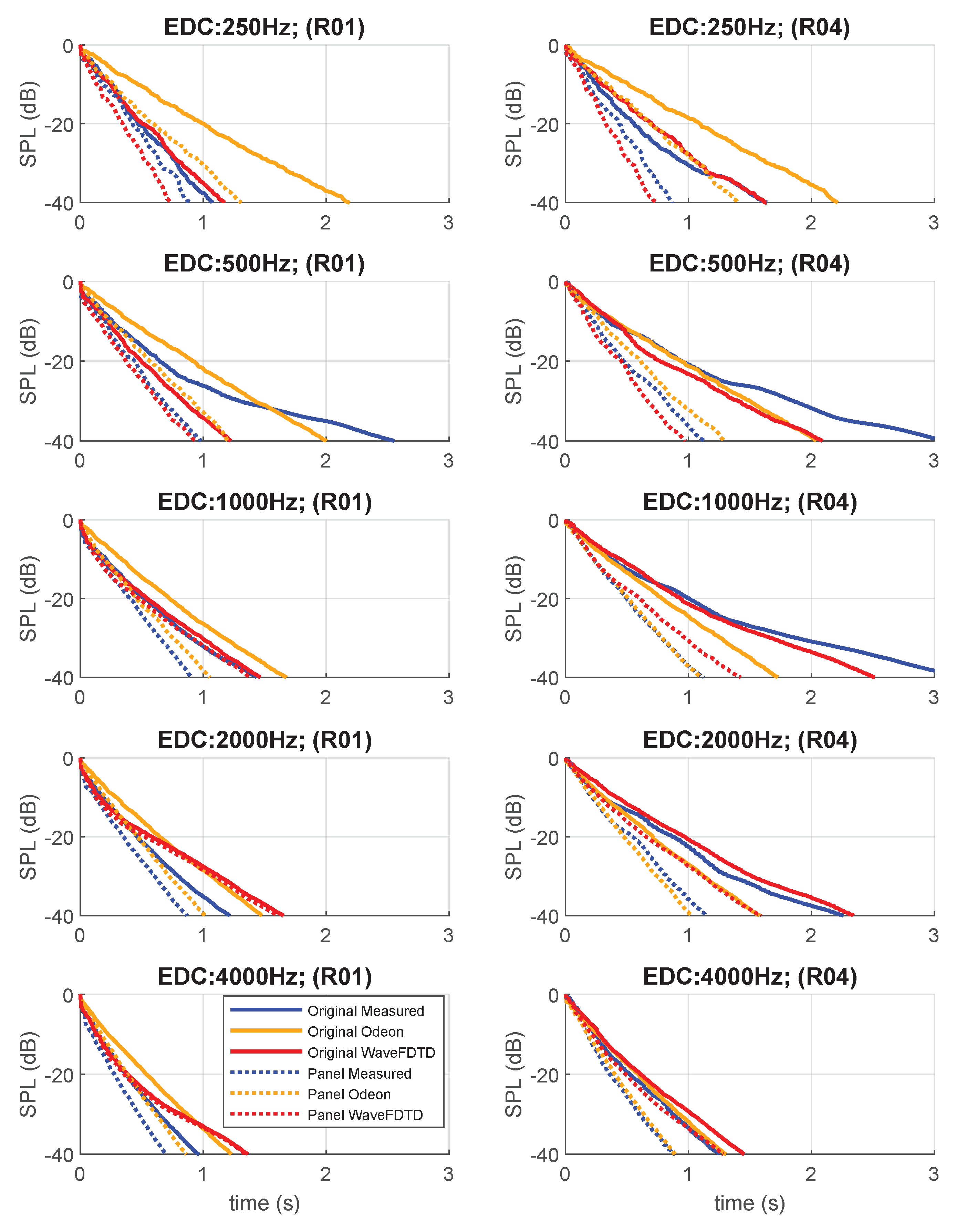
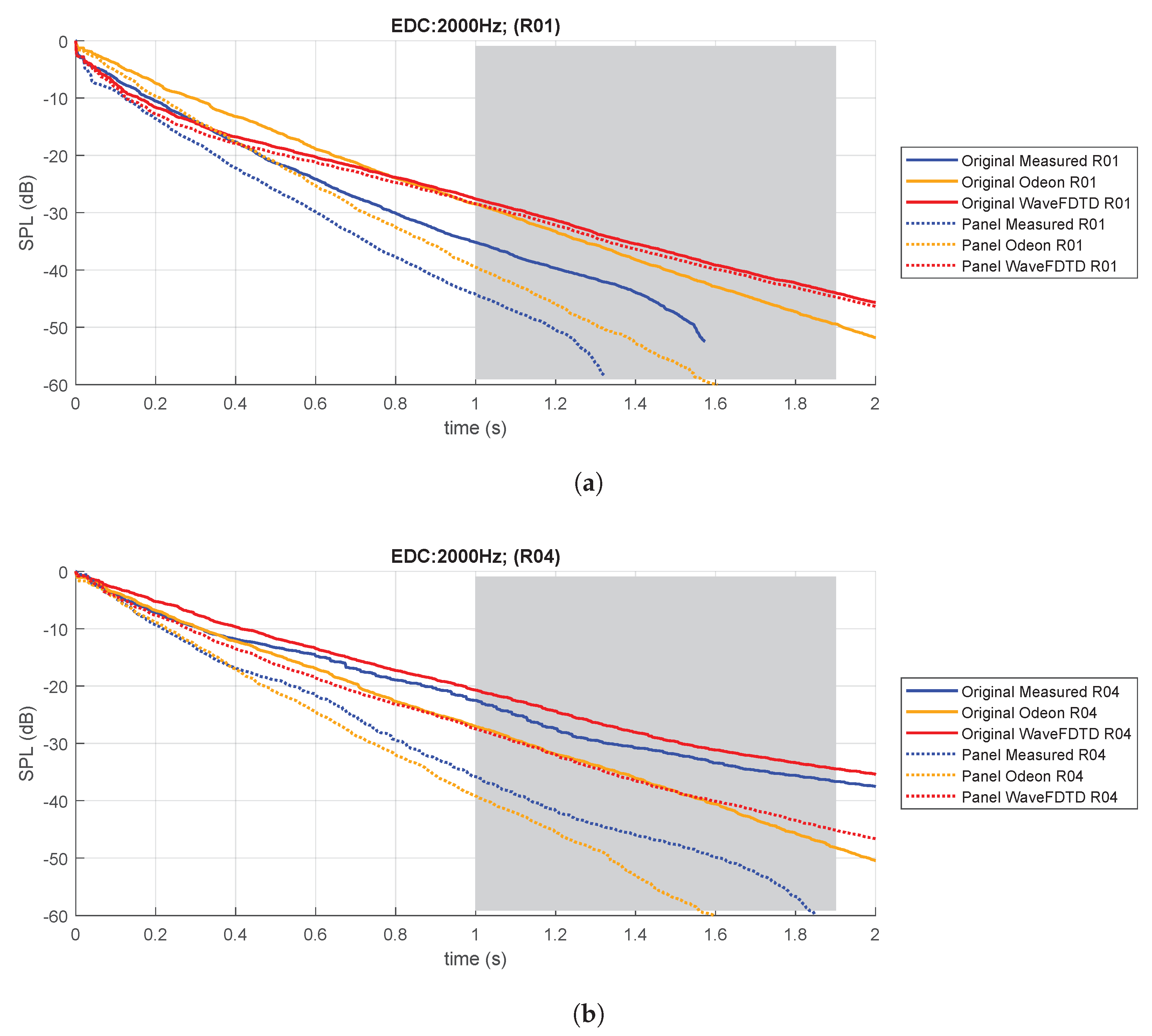
  • Energy Decay Curve: The energy decay curves were generated from the 48 kHz sampled RIR data using the ITA toolbox. The curves were normalized and plotted in dB using P r e f = 20 × 10 6 over a 40 dB reduction in SPL.

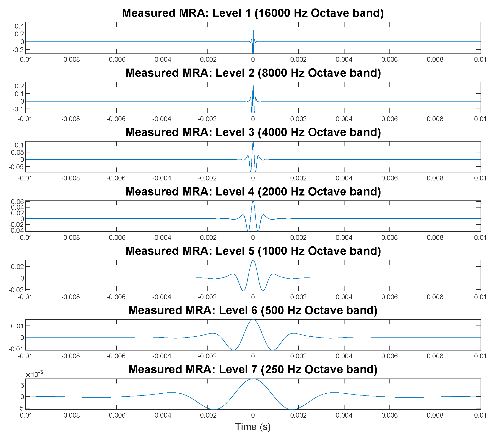
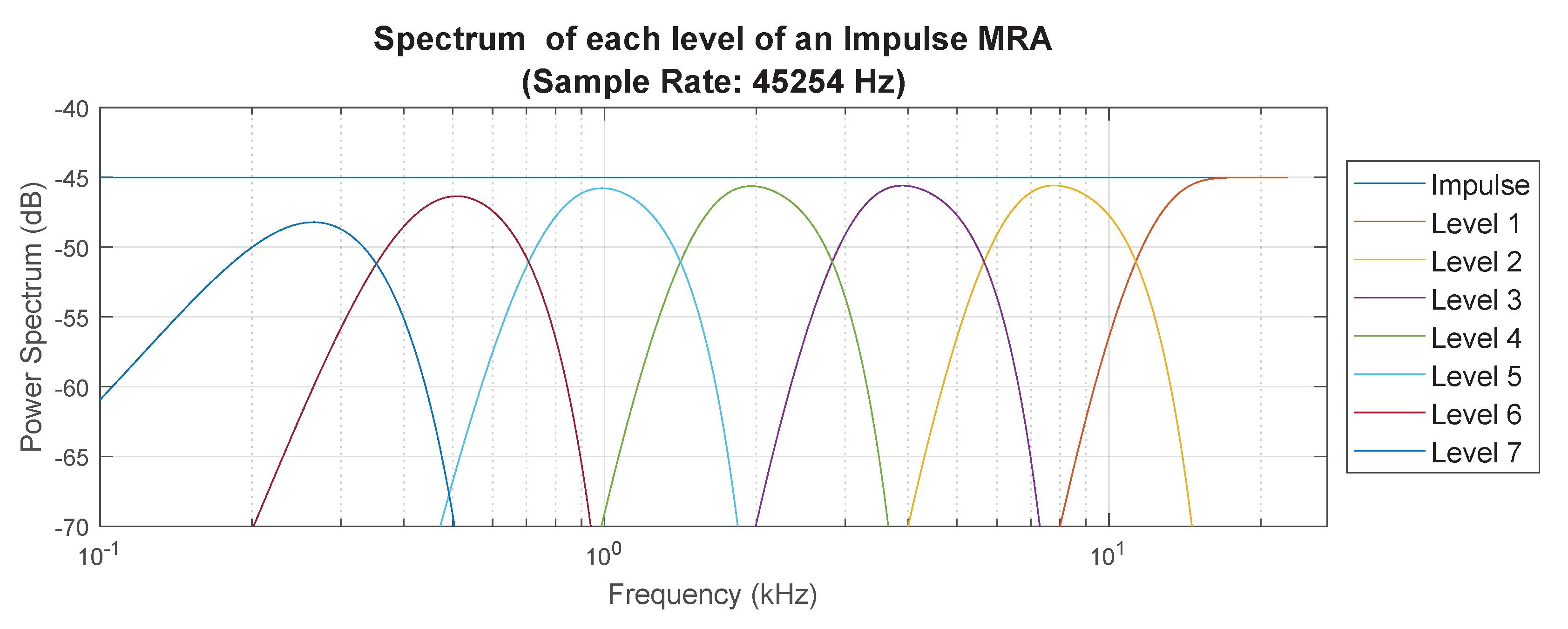
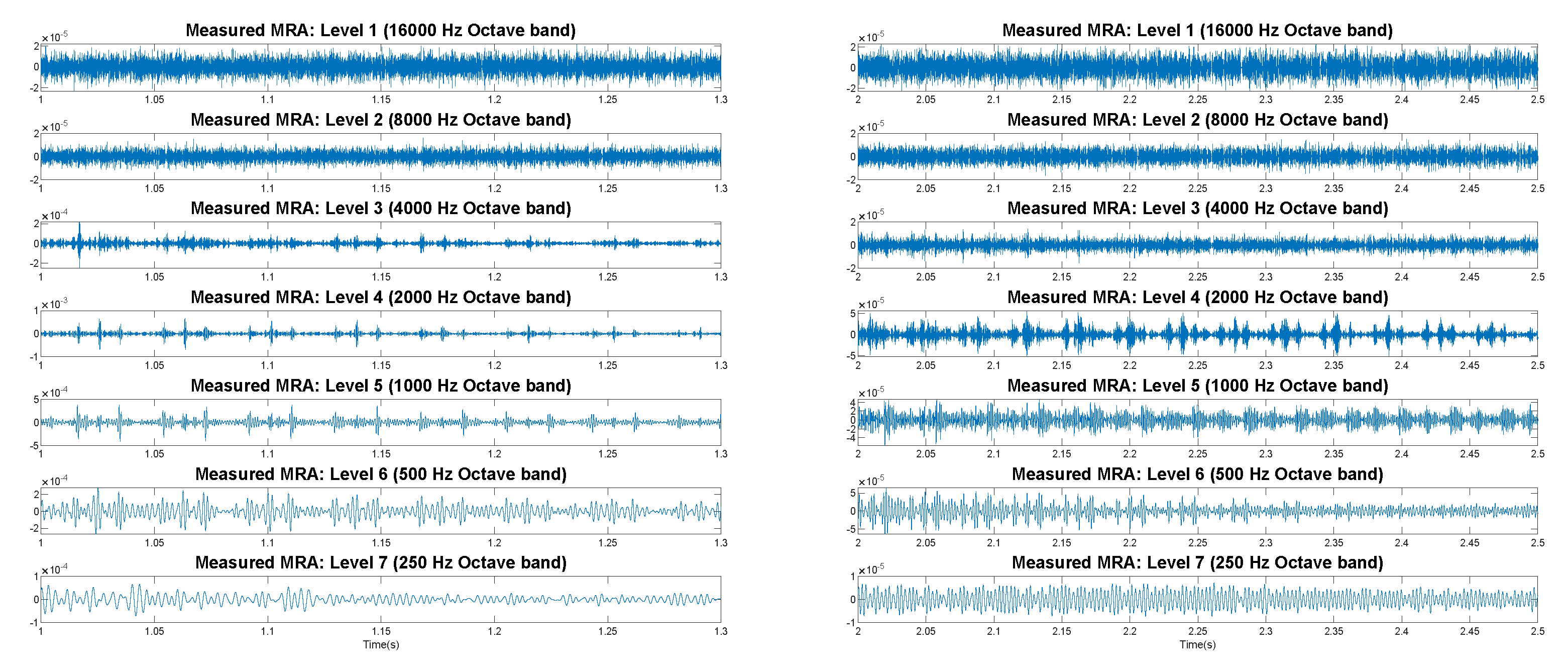
2.4. Wavelet Multi-Resolution Analysis

Because of the highly non-diffuse nature of the sound field, it was necessary to look beyond the standard room acoustics metrics such reverberation times(T(20) or T(30)) and energy decay curves in the evaluation of the sanctuary’s acoustical characteristics. To this end, the use of the discrete wavelet transform (DWT) was employed to isolate and identify specific patterns relating to the (non-diffuse) flutter echo. In particular, multi-resolution analysis (MRA) performed using the DWT was utilized for the identification of the periodic patterns in the waveforms that constitute the flutter echo.

Wavelet Selection

Before completing the MRA, the Wavelet type (family) and length had to be selected. The type and length of the wavelet used can have a significant effect on the results of the MRA, therefore, these parameters needed to be selected based on the expected shape of the signal features associated with the flutter echo signal. It was demonstrated by Wiltschko et al. [66], that there is an improvement using wavelets over traditional filtering techniques for isolating spikes or sharp peaks in measured data. Specifically, wavelet transforms are able to isolate frequency bands in the signal with less distortion of the fast peaks in the signal. Their findings are significant for applications to non-diffuse room acoustics, because the identification of patterns in the flutter echo acoustical signals requires a similar process for the isolation of peaks. Zhang et al. [67] applied statistical ANOVA analysis to the evaluate the wavelet family type and length in evaluation of fMRI data. Three different types of orthogonal, compactly supported wavelet families evaluated were evaluated in their study: Daubechies Extremal Phase (dbN), Daubechies Least Asymmetric (symN), and Coiflet (coifletN). Based on their research, the following recommendations were made:
  • The differences between the wavelet types which they applied were insignificant, therefore, any of the tested wavelet families could be applied with similar results.
  • The length of the wavelet had a significant effect on the uniformity of the results, where wavelets with longer support gave rise to more consistent results.
The efficacy of applying these recommendations to non-diffuse room acoustics was confirmed for the flutter echo triplet patterns through a direct comparison of the amplitude and quality of the signal peaks for level 4 MRA of the original measured data at receiver location R04. A single spike in a triplet was the feature extracted from the using each of the selected wavelet support lengths.
After the assessment of the wavelets, it was determined that the MRA of the RIR be performed using the MATLAB Wavelet Toolbox modwt and modwtmra commands with a Daubechies 6 (db6) wavelet (containing 6 vanishing moments and a corresponding wavelet length of 11). The result of using this wavelet family can be seen in the evaluation of the MRA of an impulse response sampled at 45,254 Hz in Figure 5.
Performing a discrete wavelet transform alone, results in phase-shifted responses at each level. To avoid this time delay, the MRA uses the detail coefficients and the low resolution approximation developed by the discrete wavelet scaling function to project the wavelet transform of the signal onto different wavelet subspaces, or levels, relating to decreasing frequency ranges. For the wavelet analysis presented here, to aid the comparison with traditional octave-band filtering, the waveform signals were resampled to 45,254 Hz. Using this sample rate, the frequency ranges of the decomposition levels relate directly to octave band frequencies as seen in Table 3.
The MRA levels of the dB6 wavelet can be seen in Figure 5 which shows the application of the wavelet to an impulse approximation (0.0442 ms triangular pulse) generated with a 45,254 Hz sample rate over −0.01 to 0.01 s.
The frequency bands of each of the MRA levels can be clearly identified in Figure 6, by comparison of the spectrum from the original signal with the spectrum of each of the MRA levels from Figure 5, demonstrating the MRA’s behavior as a linear-phase filter bank with center frequencies corresponding to each of the octave bands. Using this wavelet MRA, provides an octave band filter which retains the specific fine features associated with the periodic peaks of the flutter echo signal.

3. Results and Discussion

Using the methods described in Section 2.3 and Section 2.4, the measured and modeled RIRs were used to develop a set of figures which collectively demonstrate the unique behavior of the flutter echo in the room under investigation. These figures are presented in such a manner that comparisons between measured and modeled data can be readily made. In the initial investigation all six selected receiver locations were evaluated, both with and without panels. However, to reduce the complexity for reporting purposes, the number of receiver locations retained for each of the curves generated was reduced to two or three receiver locations. To this end, while R02 and R06 were used within the study to evaluate the response at these locations, their waveforms were considered redundant for reporting purposes, and were not included in this results section. The receiver locations and room configuration (original or with panels) in each figure was chosen to highlight specific features of the signals which demonstrate characteristics of the room’s acoustical behavior.
Rationale for the selection of receiver locations is as follows:
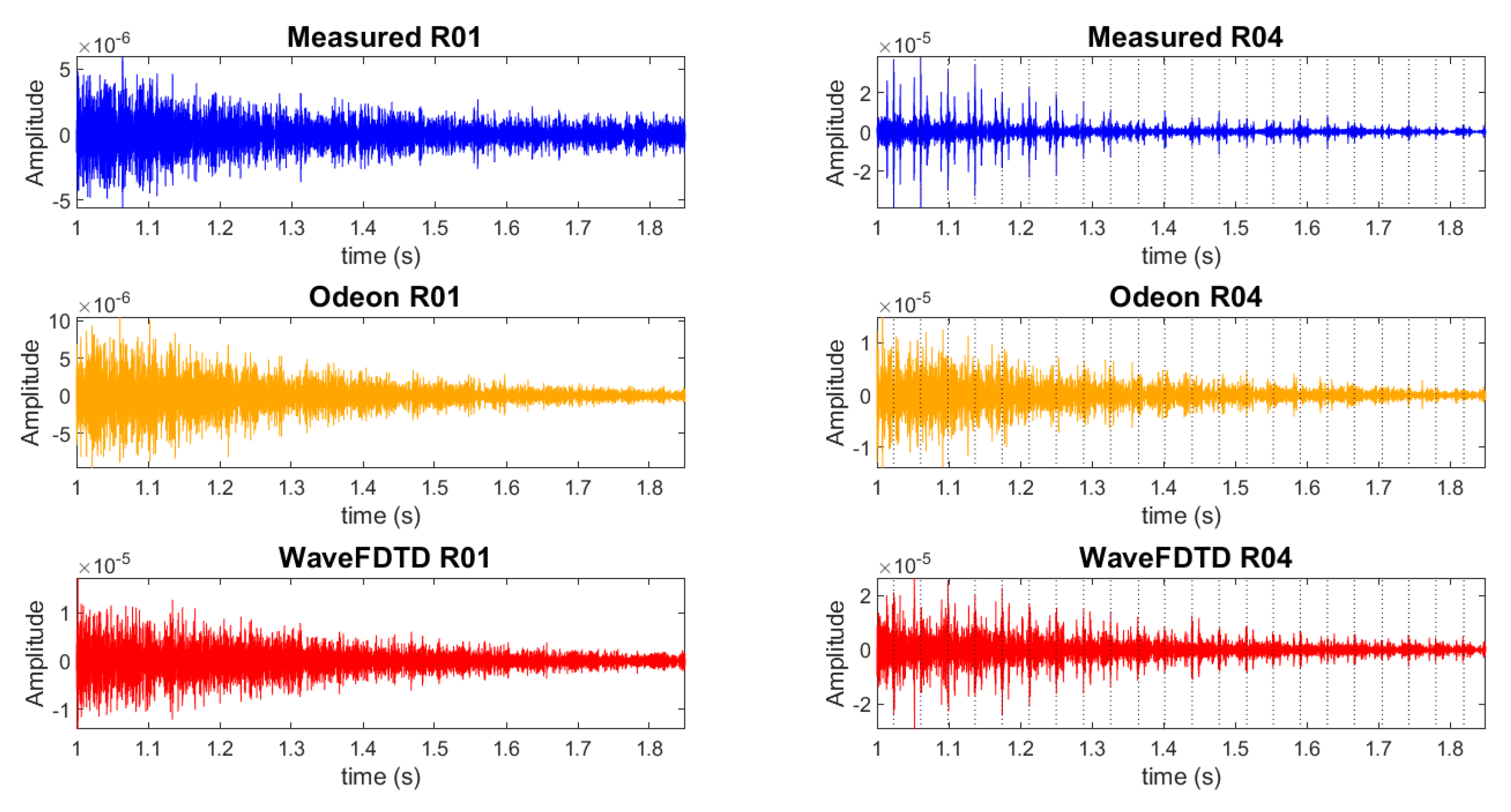
  • R01 and R04: As both of these figures are the same distance from the sound source, with one located on the aisle and the other located off the aisle, comparison between these two points demonstrates the non-diffuse nature of the room.
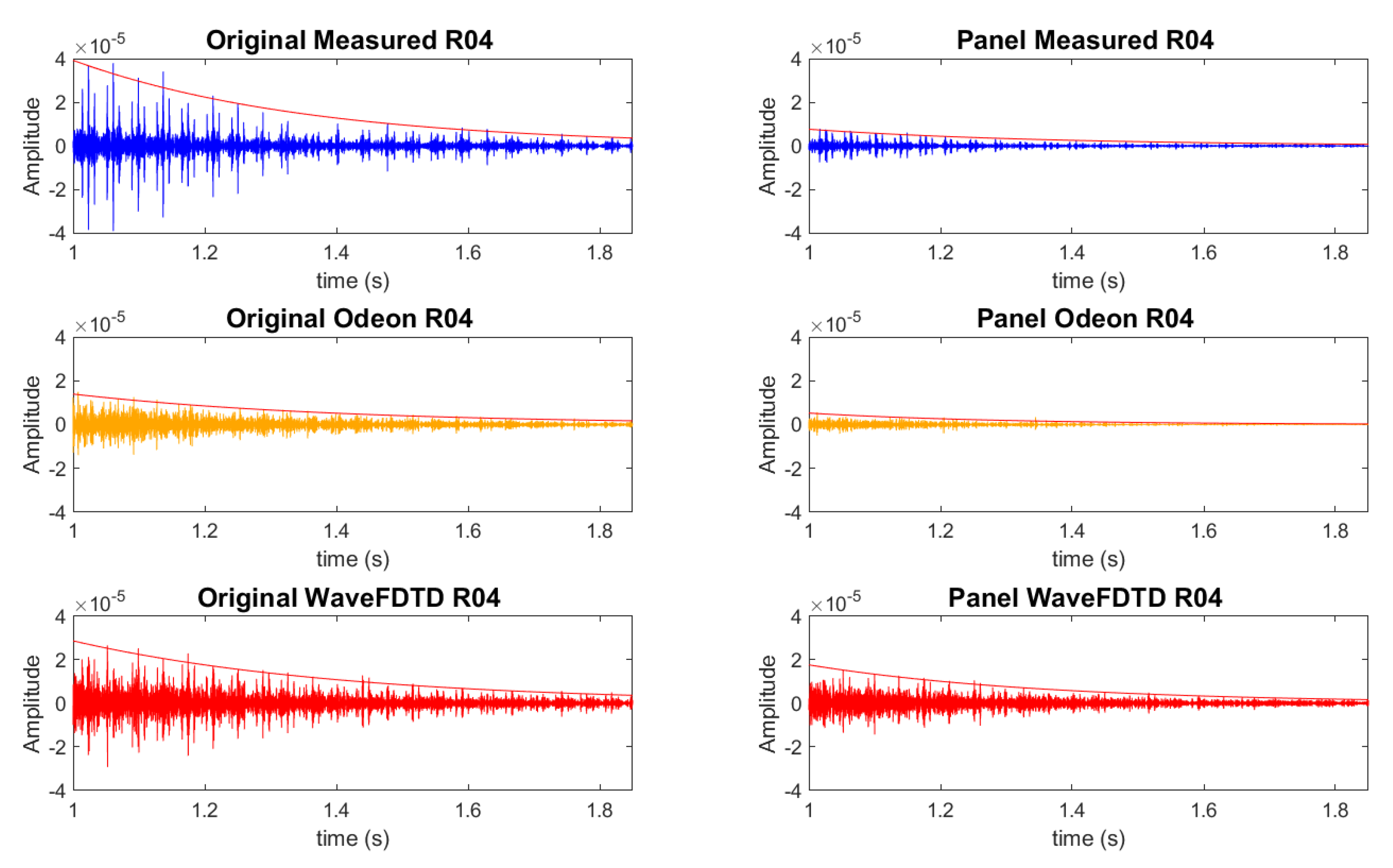
  • Original and Panel (with R01 and R04): In order to demonstrate the changes in the room acoustics as a result of the addition of acoustical panels, some figures feature side-by-side comparisons of the original room configuration and the room configured with panels as shown in Figure 4.
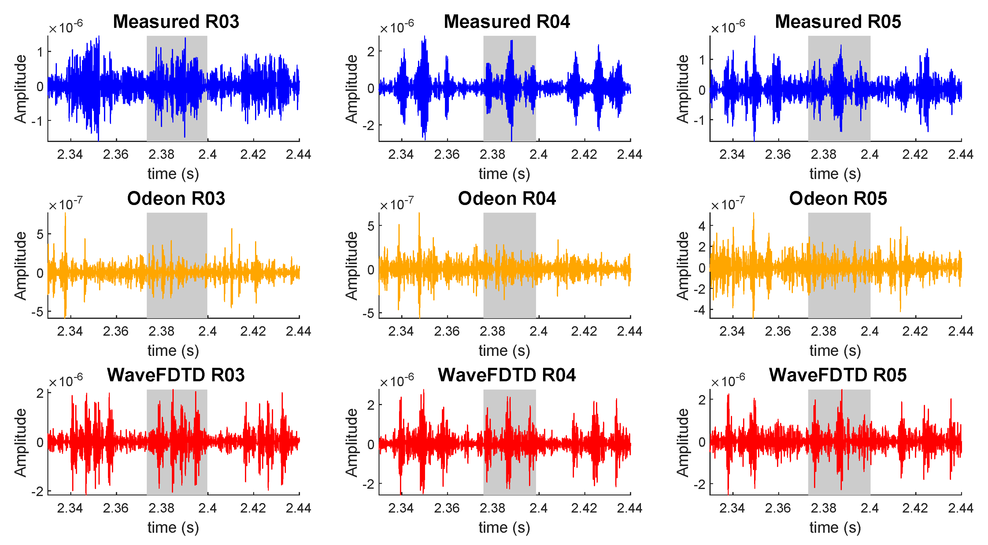
  • R03, R04 and R05: These three receiver locations represent three different heights at the same location in the room as shown in Figure 3. This comparison demonstrates the unique behavior of the flutter echo at different heights relative to the source height.

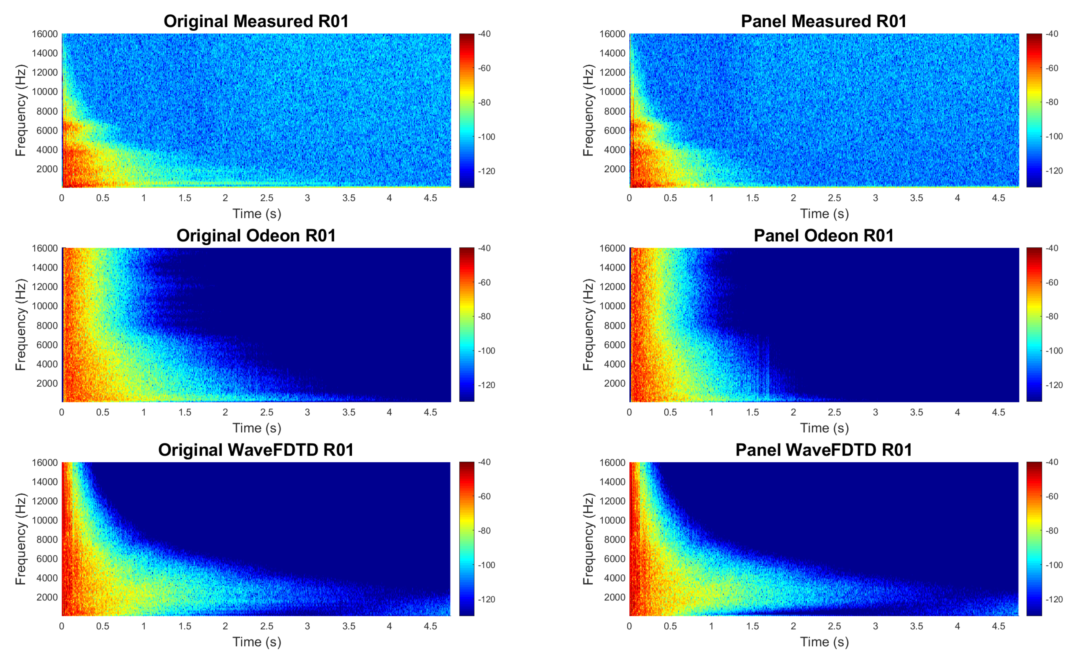
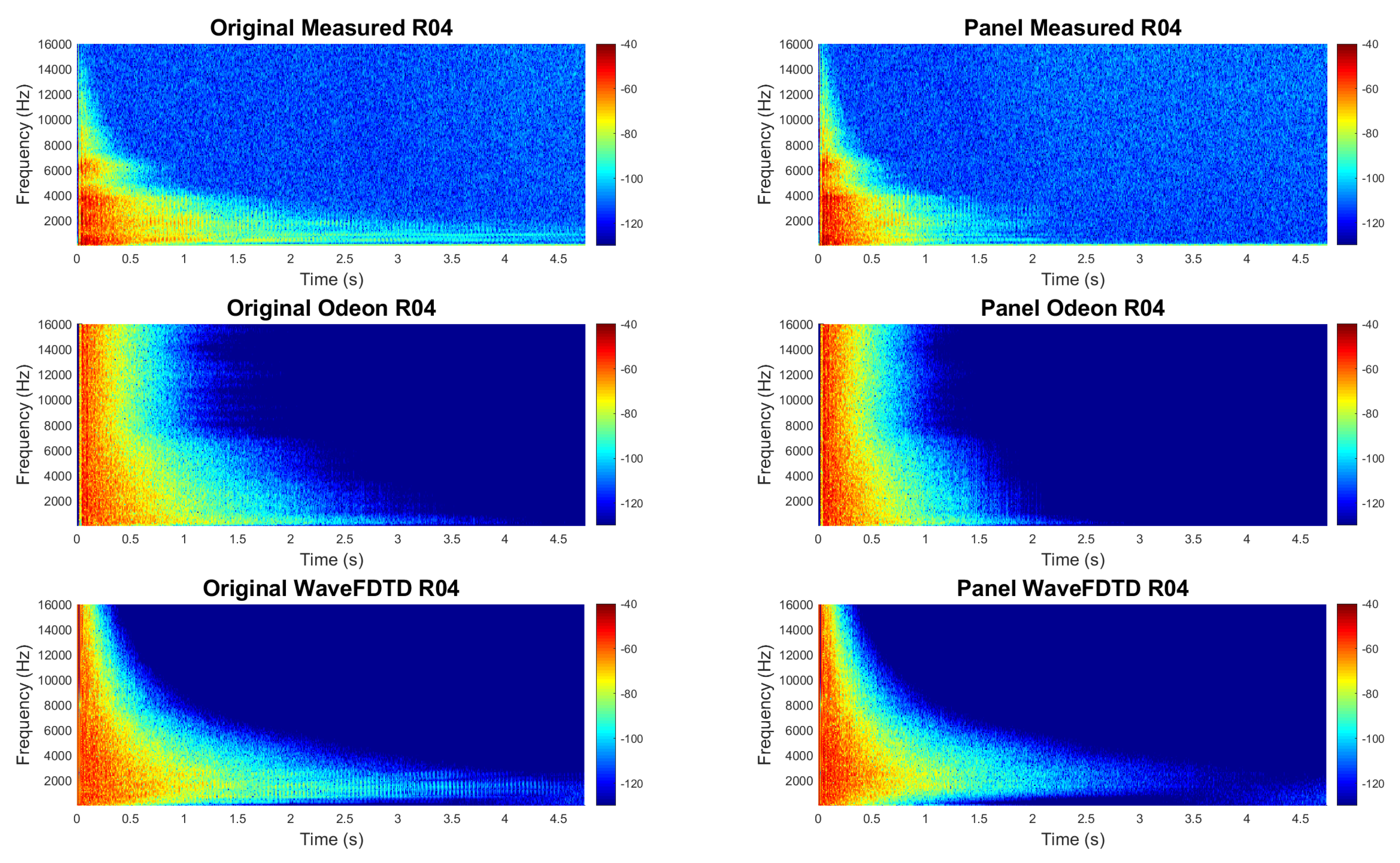
3.1. RIR Spectrogram

Spectrograms were generated for each of the selected receiver points. After evaluation of all points, receiver locations R01 and R4 were selected for comparison. Figure 7 and Figure 8 highlight the difference of the RIR on the aisle and in the audience.
Inspection of the spectrograms in each of these figures reveals key distinctions in the late decay (1.5–4.5 s) behavior between the R01 (audience) and R04 (aisle) RIR, especially in the 500–4000 Hz octave bands. These distinctions, which are most pronounced for the measured data and the wave-based model, will be further described in the following evaluation. This discussion of the spectrograms provides an overview of all of the different characteristics which will be evaluated throughout the entire results section.
  • Behavior of the room on and off the aisle: Comparison of Figure 7 and Figure 8, demonstrates the non-diffuse nature of the room. As stated earlier, both receiver points R01 and R04 are the same distance from the sound source, however, because of their location with respect to the barrel-vaulted ceiling, their spectrograms display very different behaviors.
    In high frequencies, above 4000 Hz, the measured original R01 and R04 spectrograms exhibit similar behavior, with the majority of the energy having died out by 0.5 s. Below 4000 Hz, the behavior of the two locations are quite different. In the audience, the signal dies out almost completely by 1.5 s, while in the aisle, it remains well beyond 4 s. Additionally, the signal is characterized by a periodic pattern representative of the flutter echo present in the aisle. Furthermore, along the aisle, it is possible to identify the comb filter behavior expected from a flutter echo.
  • Behavior of room before and after the addition of panels: In order to demonstrate the changes in the room acoustics as a result of the addition of acoustical panels, some figures feature side-by-side comparisons of the original room configuration and the room configured with panels as shown in Figure 1.
    Similar to what was observed in the comparison of R01 and R04, at higher frequencies (above 4000 Hz), the addition of the panels had very little effect on the spectrogram. Below 4000 Hz, in the audience area, the addition of the panels reduces the energy, such that the signal is essentially eliminated after 1.5 s. On the aisle, the effect of the panels is more pronounced, with the primary effect being to eliminate the majority of the late decay energy in the 250–2000 Hz octave bands after 2 s. The panels also have a secondary effect of reducing the amplitude of the peaks from 0.5 to 1.5 s.
    These results indicate that the panels had the desired effect of reducing the RT along the aisle without completely eliminating the spacious feel of the room promoted by the flutter echo.
  • Comparison of the GA and wave-based modeling with the measured data: The spectrograms provide a means of comparison of the similarities and distinctions between the measured data and the two different modeling techniques, GA and wave-based. Comparison between measured and modeled response before 0.5 s highlights specific early behaviors (before 0.5 s) and later behaviors. Before 0.5 s, both models contain more energy above 8 kHz than the measured data, with Odeon predicting much more sustained high frequency energy. It is important to note that above 8 kHz, both Odeon and the wave-based model use ray-tracing techniques. Also, the measured data has a band of higher energy sustained past 0.5 s around 6500 Hz, which is not identified in the wave-based model.
    Most significantly, the very distinct pattern of the flutter echo detected in measurements on the aisle in Figure 8, are clearly identified in the wave-based model, but are not present in the spectrogram of the Odeon model RIR.
In order to confirm and refine the results of the spectrograms, the RT, EDC, and fine features calculated from the RIR were observed. Results from each of these acoustic metrics are described in the following sections.

3.2. RIR Reverberation Times

Using the method described in Section 3.1, reverberation times (RT) were generated for each of the identified receiver points. Figure 9 shows the reverberation times (T(20) shown in dashed and T(30) in solid) calculated using the measured and modeled RIR data at specific receiver locations: R04, on the aisle; and R01, in the audience (both before and after the addition of the panels).
Comparison of the measured RT (blue lines) for the original room locations on and off the aisle displays the non-diffuse nature of the room. Both receiver points, R01 and R04 are at the same height and the same distance from the sound source, however, because of their location with respect to the barrel-vaulted ceiling, the reverberation times differ substantially from one another, especially in the 250–4000 Hz octave bands. The addition of the acoustical panels greatly reduces all of the elevated RTs, and results in much lower discrepancies between the on and off aisle RTs across all of the octave bands.
There is little difference between the measured T(20) and T(30) RTs after the addition of the panels, both on and off the aisle, all of the RTs are below 2 s, and at the majority of frequencies, the T(20) and T(30) RTs are nearly identical. In the original room configuration, however, the T(20) and T(30) RTs show a number of striking dissimilarities. Comparison between the T(20) and T(30) RTs in the audience indicates that there is a strange behavior occurring in the 500 Hz octave band. The T(30) RTs are consistently slightly higher than the T(20) RTs, however, in the 500 Hz octave band, T(30) is almost two seconds greater than the T(20) RT. This discrepancy warrants a closer look at the EDCs from which the RTs are calculated. This substantial difference between T(20) and T(30) RTs is even more expansive on the aisle, where the difference between the two RTs are greater than one second for the 250–1000 Hz octave bands. For frequencies greater than 1000 Hz, however, the RTs become almost identical, showing less discrepancy than these frequencies in the audience measurement.
In comparing the RTs for the modeled RIR, the wave-based model exhibits very different behavior on and off the aisle. The wave-based model does not correlate with the measured data in two aspects: first, it does not anticipate the extremely high T(30)s around 500 Hz, and secondly, it overestimates the RTs above 1000 Hz in the audience, and in the aisle after the addition of the panels. In comparing the predicted effect of adding the panes, the audience receiver location suggests little difference in the RTs with and without the panels, which is not reflective of the measured behavior. On the aisle, however, there is a large difference, with a reduction in RT for almost all frequency bands, and especially in the 250–1000 Hz bands. Although the RTs are slightly higher than the measured results in the 1000–8000 Hz octave bands, the model still does a reasonable job of estimating the reduction in the RTs on the aisle due to the addition of the panels.
The Odeon model shows very little difference between the aisle and audience receiver positions, and greatly overestimates the low frequency RTs, however it provides a close approximation of the audience RTs above 1000 Hz. The Odeon model also indicates very little change between the RTs due to the addition of the panels.

3.3. Energy Decay Curves

Prompted by the long reverberation times, and the large discrepancies between T(20) and T(30) reverberation times, energy decay curves (EDC) were evaluated for each of the selected points. As with the reverberation time calculations, receiver locations R01 and R04 were used for comparison as shown in Figure 10.
Based on the RT values, it was expected that the audience measurements would display a distinct difference between the slopes of the early and late portions of the EDC. As predicted by the RTs, the EDCs for the measured data in the audience almost always exhibit a linear decay, with the exception of the 500 Hz octave band, which demonstrates a distinct change in slope around 1 s, resulting in a much shallower curve during the late reflections, which is in keeping with the much higher T(30) prediction at that octave band.
As expected from the T(20) and T(30) results presented in Section 3.2, where the measurement T(30) values on the aisle are substantially higher than the T(20) in the 250–2000 Hz octave bands, the measured EDCs in these octave bands are also non-linear. Not only do they display an elbow around 1 s in the 500 and 1000 Hz octave bands, but they also exhibit two other non-linear characteristic behaviors. The first such characteristic is the broad ripples in the EDC, indicating variations in the late decay energy which cause the increase in the RTs in the 250 to 2000 Hz octave bands. The second non-linear characteristic feature of the flutter echo, a stepped decay in the EDC can be seen more clearly on the close-up plot of receiver R04’s 2000 Hz octave band EDC in Figure 11b. A close-up of the EDCs shown in Figure 11 shows in greater detail how the stepped decay is overlaid on the broad ripples. This stepped decay behavior has been identified in rooms with strong flutter echo [41], and indicates that there are non-diffuse features of this sound field that need to be evaluated through direct observation of the waveform, rather than simply through the use of traditional room acoustic objective metrics which assume a diffuse field. To this end, a multi-resolution wavelet analysis will be used in the following section for further comparison of flutter echoes in measurements and computer simulation results. The highlighted area of the EDC in Figure 11 indicates the time which will be highlighted in the comparisons of on and off the aisle receiver locations as well as before and after the addition of the panels.

3.4. Wavelet Multi-Resolution Analysis

As described in Section 2.4, when applied to the measured RIR using an appropriate wavelet, the MRA of the signal can be used to isolate features that occur at specific frequency bands, making the DWT useful in peak detection and pattern recognition in acoustical signals. Based on the spectrograms shown in Section 3.1, it was identified that the flutter echo was comprised of repeating patterns of peaks which persisted most strongly in the 1 and 2 kHz frequency bands.
To support the observation from the spectrogram that the flutter echo was most distinct in these frequency bands, wavelet MRA scale levels 1 through 7 of R04 measured data were evaluated during mid and (t > 1 s) and late reflections (t > 2 s) for patterns related to the flutter echo in Figure 12. Observation of the MRA confirms that the features of the flutter echo are most pronounced in levels 4 through 6, relating to the 500–2000 Hz octave bands (for data sampled at 45.254 kHz). In particular, based on the distinct peaks of the triplets identified in the level 4 MRA scale, representing the 2000 Hz frequency band, this level was selected to represent the triplet pattern generated by the flutter echo in each of the figures generated using the wavelet MRA.
Throughout the rest of this analysis, Level 4 MRA will be used to demonstrate the fine features of the flutter echo and provide comparisons between measured and modeled results for signals on and off the aisle, before and after the addition of acoustical panels, and at various receiver heights.

3.4.1. Comparison of Flutter Echo On and Off the Aisle

In Figure 13, the RIR is plotted at 1 s both on and off the aisle, for the measured and modeled responses. The presence of the flutter echo is much more distinctly identifiable on the aisle (R04) than it is off of the aisle (R01), with the fine details of the flutter echo apparent as a triplet pattern with the middle peak characteristically being the largest amplitude. The dotted lines on the plots for R04 identify the middle peak of the triplets in the measured signal. The locations of these peaks were determined automatically using the MATLAB findpeaks command with a minimum peak prominence of 10 × 10 7 , and a minimum peak distance of 1600.
Comparison with the modeled results show that the peaks of the triplets in the wave-based model line up closely with the dotted lines that were identified from the measured data. The Odeon model, on the other hand, does not exhibit the clear triplet peaks with the correct timing in the same way that the wave-based model does.

3.4.2. Comparison of Flutter Echo Before and After the Addition of Panels

Comparison of the change in the flutter echo behavior as a result of the addition of the acoustical panels can be observed in Figure 14. This figure compares the response after 1s on the aisle at R04, both in the original configuration and after the addition of the panels. The red lines included in each figure are calculated using an exponential curve fit of the peaks of each of the triplets, and are provided simply to aid in the visualization of how the peak amplitudes of the signal decay over the time window shown.
As observed in Figure 13, there is a distinct flutter echo pattern in the measured data from the original room configuration. This triplet pattern is also clearly present in the measured data after the addition of the panels. Based on this comparison, it can be seen that the primary effect of the treatment is a substantial reduction of the amplitude of the flutter echo in the RIR, without eliminating the triplet structure.
Comparison of the behavior of both of the models demonstrates a similar result, with each of the models displaying a marked decrease in the amplitude of the signal, while still retaining the predicted structure of the echoes. The fine features of the triplet pattern are more clearly identified in the wave-based model in the original configuration, and therefore, are more clearly identifiable after the addition of the panels as well.

3.4.3. Structure of Triplets Based on Receiver Height

Although the structure of the flutter echo is identifiable throughout the RIR, it can be seen most clearly in the late reflections t > 2 s. Observation of the RIR waveform in Figure 15 demonstrate the changes in the fine structure of the flutter echo at different receiver points. This structure is directly related to the location of the receiver relative to the source in relation to the reflective surfaces. Specifically in this case, because the reflective surfaces are the tiled aisle and the curved ceiling, when the receiver is at nearly the same height as the sound source (at R04 the receiver is 0.2 m below the source), the flutter echo pattern takes on the very distinct triplet pattern as seen in the R04 plots of Figure 15, with the center peak being higher in amplitude than the outer peaks, due to constructive interference from the ceiling and floor reflections.
When the receiver is below the source, the peaks become spread out, as the two wave fronts which caused the center peak in the R04 triplet pattern, are now separated, to form a wider structure. This structure can be seen most clearly in the wave-based model for R03 which is located 0.7 m from the source. In R05, the distinct center peak of the triplet pattern is still visible, but it is slightly wider because its height, 0.3 m above the source is slightly further from the source than R04. Once again, the fine features of the structure of the flutter echo at this height is clearly replicated by the wave-based model, whereas the Odeon model exhibits some of these features, but they are greatly diminished in amplitude, and are not as accurately reproduced.
Results of spectrograms, T(20) and T(30) calculations, energy decay curves, and wavelet multi-resolution analysis have been presented in this section, providing a means to discuss both the unique features of the flutter echo itself, and the efficacy of GA and wave-based modeling to reproduce these features.

4. Conclusions

This article investigated the acoustics of a barrel-vaulted sanctuary with a significant flutter echo along the aisle, and its later acoustical remediation. Through the use of spectrograms, T(20) and T(30) calculations, energy decay curves, and wavelet multi-resolution analysis, the broad behaviors and the fine details of the acoustical behavior of a non-diffuse room exhibiting a distinct flutter echo have been evaluated. This evaluation included comparison of the behavior on and off the center aisle of the room, before and after the addition of acoustical panels, and identification of similarities between measured data and two different acoustical modeling techniques. Within these analyses, GA and wave-based simulated RIRs were compared to measurements. There were various uncertainties in computer model absorption and scattering coefficients, but this non-diffuse room did not warrant a detailed calibration through diffuse-field objective metrics. Despite this, the simulated results showed agreement with fine features of flutter echoes along aisle, with wave-based results modeling the fine details of the echo more accurately than GA results. However, GA results showed better agreement in the differences between off-aisle decay times and curves before and after remediation, as compared to measurements. The discrepancy in off-aisle decay time modeling could be attributed to the limitations of a locally-reactive boundary condition (angle-dependent absorption) in the modeling of panel absorbers (which themselves deviate from the locally-reactive model) by the wave-based model. The applied absorption in the GA model, however, is a combination of angle-dependent and random-incidence absorption [53], which is perhaps better suited to modeling of panel absorbers. The particular behaviors of both models in regards to off-aisle decay times in this space could be the topic of future work. Future work could also include a perceptual evaluation of measured and simulated responses, to better refine quantitative similarities in reproduction of flutter echoes, along with the use of alternative commercial GA softwares.

Author Contributions

Conceptualization and methodology, H.L. and B.H.; software, B.H.; simulation, H.L. and B.H.; measurement and data curation, H.L.; writing—original draft preparation, H.L. and B.H.; writing—review and editing, H.L. and B.H. All authors have read and agreed to the published version of the manuscript.

Funding

This research was funded in part by ERC grant number ERC-PoC-2016-WRAM and EPSRC grant number EP/R005001/1. Funding was also provided through the Dr. Nuala McGann Drescher Affirmative Action/Diversity Leave and SUNY New Paltz Student Undergraduate Research Experience.

Acknowledgments

The authors wish to thank Claus Christensen for his help on choosing optimal simulation parameters within Odeon software for this room along with Anne Balant of SUNY New Paltz for her invaluable help in collecting and interpreting the measured data. Additionally, the authors acknowledge Vassar College and Seth Bard of the IBM Hudson Valley Acoustics Lab for the use of measurement equipment, as well as Christ the King Charismatic Church for access to the space.

Conflicts of Interest

The authors declare no conflict of interest.

References

  1. Krokstad, A.; Strom, S.; Sørsdal, S. Calculating the acoustical room response by the use of a ray tracing technique. J. Sound Vib. 1968, 8, 118–125. [Google Scholar] [CrossRef]
  2. Schroeder, M.R. Computer models for concert hall acoustics. Am. J. Phys. 1973, 41, 461–471. [Google Scholar] [CrossRef]
  3. Cremer, L.; Müller, H.; Schultz, T. Principles and Applications of Room Acoustics, Volume 1; Applied Science Publishers Ltd.: London, UK, 1982. [Google Scholar]
  4. Vorländer, M. Simulation of the transient and steady-state sound propagation in rooms using a new combined ray-tracing/image-source algorithm. J. Acoust. Soc. Am. 1989, 86, 172. [Google Scholar] [CrossRef]
  5. Savioja, L.; Svensson, U.P. Overview of geometrical room acoustic modeling techniques. J. Acoust. Soc. Am. 2015, 138, 708–730. [Google Scholar] [CrossRef] [Green Version]
  6. Dalenbäck, B.I. A New Model for Room Acoustic Prediction and Auralization. Ph.D. Thesis, Chalmers University of Technology, Gothenburg, Sweden, 1995. [Google Scholar]
  7. Naylor, G.M. ODEON—Another hybrid room acoustical model. Appl. Acoust. 1993, 38, 131–143. [Google Scholar] [CrossRef]
  8. Shuku, T.; Ishihara, K. The analysis of the acoustic field in irregularly shaped rooms by the finite element method. J. Sound Vib. 1973, 29, 67–76, IN1. [Google Scholar] [CrossRef]
  9. Chiba, O.; Kashiwa, T.; Shimoda, H.; Kagami, S.; Fukai, I. Analysis of sound fields in three dimensional space by the time-dependent finite-difference method based on the leap frog algorithm. J. Acoust. Soc. Jpn. 1993, 49, 551–562. [Google Scholar]
  10. Botteldooren, D. Acoustical finite-difference time-domain simulation in a quasi-Cartesian grid. J. Acoust. Soc. Am. 1994, 95, 2313–2319. [Google Scholar] [CrossRef]
  11. Savioja, L.; Rinne, T.J.; Takala, T. Simulation of Room Acoustics with a 3-D finite difference mesh. In Proceedings of the International Computer Music Conference (ICMC), Aarhus, Denmark, 12–17 September 1994; pp. 463–466. [Google Scholar]
  12. Kowalczyk, K.; van Walstijn, M. Room acoustics simulation using 3-D compact explicit FDTD schemes. IEEE Trans. Audio Speech Lang. Process. 2011, 19, 34–46. [Google Scholar] [CrossRef] [Green Version]
  13. Hargreaves, J.A. Time Domain Boundary Element Method for Room Acoustics. Ph.D. Thesis, University of Salford, Salford, UK, 2007. [Google Scholar]
  14. Sakuma, T.; Sakamoto, S.; Otsuru, T. Computational Simulation in Architectural and Environmental Acoustics; Springer: Berlin, Germany, 2014. [Google Scholar]
  15. Savioja, L. Real-time 3D finite-difference time-domain simulation of low-and mid-frequency room acoustics. In Proceedings of the International Conference on Digital Audio Effects (DAFx), Graz, Austria, 6–10 September 2010; Volume 1, p. 75. [Google Scholar]
  16. Webb, C.J.; Bilbao, S. Computing room acoustics with CUDA - 3D FDTD schemes with boundary losses and viscosity. In Proceedings of the IEEE International Conference on Acoustics, Speech, and Signal Processing (ICASSP), Prague, Czech Republic, 22–27 May, 2011; pp. 317–320. [Google Scholar]
  17. López, J.J.; Carnicero, D.; Ferrando, N.; Escolano, J. Parallelization of the finite-difference time-domain method for room acoustics modelling based on CUDA. Math. Comput. Model. 2013, 57, 1822–1831. [Google Scholar] [CrossRef]
  18. Van Mourik, J.; Murphy, D. Explicit higher-order FDTD schemes for 3D room acoustic simulation. IEEE/ACM Trans. Audio Speech Lang. Process. 2014, 22, 2003–2011. [Google Scholar] [CrossRef]
  19. Spa, C.; Rey, A.; Hernandez, E. A GPU implementation of an explicit compact FDTD algorithm with a digital impedance filter for room acoustics applications. IEEE/ACM Trans. Audio Speech Lang. Process. 2015, 23, 1368–1380. [Google Scholar] [CrossRef]
  20. Saarelma, J.; Califa, J.; Mehra, R. Challenges of Distributed Real-Time Finite-Difference Time-Domain Room Acoustic Simulation for Auralization. In Proceedings of the AES International Conference on Spatial Reproduction-Aesthetics and Science, Tokyo, Japan, 7–9 August 2018. [Google Scholar]
  21. Saarelma, J.; Savioja, L. An Open Source Finite difference Time-domain Solver for Room Acoustics Using Graphics Processing Units. In Proceedings of the Forum Acusticum, Krakow, Poland, 7–12 September 2014. [Google Scholar]
  22. Weitze, C.A.; Rindel, J.H.; Christensen, C.L.; Gade, A.C. The acoustical history of Hagia Sophia revived through computer simulation. In Proceedings of the Forum Acusticum, Sevilla, Spain, 16–20 September 2002. [Google Scholar]
  23. Postma, B.N.; Katz, B.F. Perceptive and objective evaluation of calibrated room acoustic simulation auralizations. J. Acoust. Soc. Am. 2016, 140, 4326–4337. [Google Scholar] [CrossRef] [PubMed]
  24. Boren, B.; Longair, M.; Orlowski, R. Acoustic simulation of renaissance venetian churches. Acoust. Pract. 2013, 1, 17–28. [Google Scholar] [CrossRef]
  25. Foteinou, A.; Murphy, D.T. Perceptual validation in the acoustic modeling and auralisation of heritage sites: The acoustic measurement and modelling of St Margaret’s Church, York, UK’. In Proceedings of the Conference on the Acoustics of Ancient Theatres, Patras, Greece, 18–21 September 2011; pp. 18–21. [Google Scholar]
  26. Oxnard, S.; Murphy, D.T. Achieving convolution-based reverberation through use of geometric acoustic modeling techniques. In Proceedings of the 15th International Conference on Digital Audio Effects (DAFx12), York, UK, 17–21 September 2012; p. 105. [Google Scholar]
  27. Alvarez-Morales, L.; Martellotta, F. A geometrical acoustic simulation of the effect of occupancy and source position in historical churches. Appl. Acoust. 2015, 91, 47–58. [Google Scholar] [CrossRef]
  28. Van Mourik, J.; Oxnard, S.; Foteinou, A.; Murphy, D.T. Hybrid acoustic modelling of historic spaces using blender. In Proceedings of the Forum Acusticum, Krakow, Poland, 7–12 September 2014. [Google Scholar]
  29. Oxnard, S. Efficient Hybrid Virtual Room Acoustic Modelling. Ph.D. Thesis, University of York, York, UK, 2016. [Google Scholar]
  30. D’Orazio, D.; De Cesaris, S.; Morandi, F.; Garai, M. The aesthetics of the Bayreuth Festspielhaus explained by means of acoustic measurements and simulations. J. Cult. Herit. 2018, 34, 151–158. [Google Scholar] [CrossRef]
  31. Azad, H.; Ketabi, R.; Siebein, G. A Study of Diffusivity in Concert Halls Using Large Scale Acoustic Wave-Based Modeling and Simulation. In Proceedings of the 47th International Congress and Exposition on Noise Control Engineering, Inter-Noise 2018, Chicago, IL, USA, 26–29 August 2018; pp. 5431–5442. [Google Scholar]
  32. D’Orazio, D.; Rovigatti, A.; Garai, M. The Proscenium of Opera Houses as a Disappeared Intangible Heritage: A Virtual Reconstruction of the 1840s Original Design of the Alighieri Theatre in Ravenna. Acoustics 2019, 1, 694–710. [Google Scholar] [CrossRef] [Green Version]
  33. Hornikx, M. Acoustic modelling of indoor and outdoor spaces. J. Build. Perform. Simul. 2015, 8, 1–2. [Google Scholar] [CrossRef] [Green Version]
  34. Shtrepi, L. Investigation on the diffusive surface modeling detail in geometrical acoustics based simulations. J. Acoust. Soc. Am. 2019, 145, EL215–EL221. [Google Scholar] [CrossRef] [Green Version]
  35. Iannace, G.; Trematerra, A.; Masullo, M. The large theatre of Pompeii: Acoustic evolution. Build. Acoust. 2013, 20, 215–227. [Google Scholar] [CrossRef]
  36. Lokki, T.; Southern, A.; Siltanen, S.; Savioja, L. Acoustics of Epidaurus–studies with room acoustics modelling methods. Acta Acust. United Acust. 2013, 99, 40–47. [Google Scholar] [CrossRef] [Green Version]
  37. Bo, E.; Shtrepi, L.; Pelegrín Garcia, D.; Barbato, G.; Aletta, F.; Astolfi, A. The Accuracy of Predicted Acoustical Parameters in Ancient Open-Air Theatres: A Case Study in Syracusae. Appl. Sci. 2018, 8, 1393. [Google Scholar] [CrossRef] [Green Version]
  38. Rindel, J.H. The use of computer modeling in room acoustics. J. Vibroeng. 2000, 3, 219–224. [Google Scholar]
  39. Maa, D.Y. The flutter echoes. J. Acoust. Soc. Am. 1941, 13, 170–178. [Google Scholar] [CrossRef]
  40. Morse, P.M. Vibration and Sound; McGraw-Hill: New York, NY, USA, 1948; Volume 2. [Google Scholar]
  41. Martellotta, F.; Álvarez-Morales, L.; Girón, S.; Zamarreño, T. An investigation of multi-rate sound decay under strongly non-diffuse conditions: The crypt of the cathedral of Cadiz. J. Sound Vib. 2018, 421, 261–274. [Google Scholar] [CrossRef]
  42. Moreno, A.; Zaragoza, J.G.; Alcantarilla, F. Generation and suppression of flutter echoes in spherical domes. J. Acoust. Soc. Jpn. (E) 1981, 2, 197–202. [Google Scholar] [CrossRef] [Green Version]
  43. Lai, H.L.; Balant, A.C.; Foote, D.J. Case study: Measurement and treatment of severe flutter echo caused by a barrel-vaulted sanctuary ceiling. Noise Control. Eng. J. 2019, 67, 380–393. [Google Scholar] [CrossRef]
  44. Hamilton, B.; Webb, C.J.; Fletcher, N.D.; Bilbao, S. Finite difference room acoustics simulation with general impedance boundaries and viscothermal losses in air: Parallel implementation on multiple GPUs. In Proceedings of the International Symposium on Music and Room Acoustics (ISMRA), La Plata, Argentina, 11–13 September 2016. [Google Scholar]
  45. Lai, H.L.; Foote, D.J. Measurement, visualization, and modeling of acoustics of a barrel-vaulted sanctuary. J. Acoust. Soc. Am. 2017, 141, 3777. [Google Scholar] [CrossRef]
  46. ISO. Acoustics—Measurement of Room Acoustic Parameters—Part 1: Performance Spaces; ISO 3382-1:2009; International Organization for Standardization: Geneva, Switzerland, 2009. [Google Scholar]
  47. Kuttruff, H. Room Acoustics; CRC Press: Boca Raton, FL, USA, 2009. [Google Scholar]
  48. Cox, T.J.; Dalenback, B.I.; D’Antonio, P.; Embrechts, J.J.; Jeon, J.Y.; Mommertz, E.; Vorländer, M. A tutorial on scattering and diffusion coefficients for room acoustic surfaces. Acta Acust. United Acust. 2006, 92, 1–15. [Google Scholar]
  49. Pierce, A.D. Acoustics: An Introduction to its Physical Principles and Applications; McGraw-Hill: New York, NY, USA, 1989. [Google Scholar]
  50. Keller, J.B. Geometrical theory of diffraction. J. Opt. Soc. Am. 1962, 52, 116. [Google Scholar] [CrossRef]
  51. Svensson, U.P.; Fred, R.I.; Vanderkooy, J. An analytic secondary source model of edge diffraction impulse responses. J. Acoust. Soc. Am. 1999, 106, 2331–2344. [Google Scholar] [CrossRef] [Green Version]
  52. Schröder, D. Physically Based Real-Time Auralization of Interactive Virtual Environments; Logos Verlag Berlin GmbH: Berlin, Germany, 2011; Volume 11. [Google Scholar]
  53. Odeon A/S. Odeon Room Acoustics Software, User Manual; Version 15; Odeon A/S: Lyngby, Denmark, 2018. [Google Scholar]
  54. Heinz, R. Binaural room simulation based on an image source model with addition of statistical methods to include the diffuse sound scattering of walls and to predict the reverberant tail. Appl. Acoust. 1993, 38, 145–159. [Google Scholar] [CrossRef]
  55. Vorländer, M. Computer simulations in room acoustics: Concepts and uncertainties. J. Acoust. Soc. Am. 2013, 133, 1203–1213. [Google Scholar] [CrossRef] [PubMed]
  56. Vorländer, M. Auralization: Fundamentals of Acoustics, Modelling, Simulation, Algorithms and Acoustic Virtual Reality; Springer Science & Business Media: Berlin/Heidelberg, Germany, 2007. [Google Scholar]
  57. Hairer, E.; Lubich, C.; Wanner, G. Geometric numerical integration illustrated by the Störmer–Verlet method. Acta Numer. 2003, 12, 399–450. [Google Scholar] [CrossRef] [Green Version]
  58. Hamilton, B.; Webb, C.J.; Gray, A.; Bilbao, S. Large stencil operations for GPU-based 3-D acoustics simulations. In Proceedings of the International Conference on Digital Audio Effects (DAFx), Trondheim, Norway, 30 November–3 December 2015. [Google Scholar]
  59. Bilbao, S. Modeling of Complex Geometries and Boundary Conditions in Finite Difference/Finite Volume Time Domain Room Acoustics Simulation. IEEE Trans. Audio Speech Lang. Process. 2013, 21, 1524–1533. [Google Scholar] [CrossRef] [Green Version]
  60. Bilbao, S.; Hamilton, B.; Botts, J.; Savioja, L. Finite Volume Time Domain Room Acoustics Simulation under General Impedance Boundary Conditions. IEEE/ACM Trans. Audio Speech Lang. Process. 2016, 24, 161–173. [Google Scholar] [CrossRef] [Green Version]
  61. Bilbao, S.; Hamilton, B. Wave-based Room Acoustics Simulation: Explicit/Implicit Finite Volume Modeling of Viscothermal Losses and Frequency-dependent Boundaries. J. Audio Eng. Soc. 2017, 65, 78–89. [Google Scholar] [CrossRef]
  62. Hamilton, B. Finite Difference and Finite Volume Methods for Wave-based Modelling of Room Acoustics. Ph.D. Thesis, University of Edinburgh, Edinburgh, UK, 2016. [Google Scholar]
  63. Hamilton, B.; Webb, C.J. Room Acoustics Modelling Using GPU-accelerated Finite Difference and Finite Volume Methods on a Face-centered Cubic Grid. In Proceedings of the International Conference on Digital Audio Effects (DAFx), Maynooth, Ireland, 2–5 September 2013; pp. 336–343. [Google Scholar]
  64. Smith, J.O. Digital Audio Resampling Home Page. 2002. Available online: http://ccrma.stanford.edu/~jos/resample/ (accessed on 17 October 2019).
  65. Berzborn, M.; Bomhardt, R.; Klein, J.; Richter, J.G.; Vorländer, M. The ITA-Toolbox: An open source MATLAB toolbox for acoustic measurements and signal processing. In Proceedings of the 43th Annual German Congress on Acoustics, Kiel, Germany, 6–9 March 2017. [Google Scholar]
  66. Wiltschko, A.B.; Gage, G.J.; Berke, J.D. Wavelet filtering before spike detection preserves waveform shape and enhances single-unit discrimination. J. Neurosci. Methods 2008, 173, 34–40. [Google Scholar] [CrossRef] [Green Version]
  67. Zhang, Z.; Telesford, Q.K.; Giusti, C.; Lim, K.O.; Bassett, D.S. Choosing wavelet methods, filters, and lengths for functional brain network construction. PLoS ONE 2016, 11, e0157243. [Google Scholar] [CrossRef]
Figure 1. (left) photograph of Christ the King (CTK) church taken after remediation. The main aisle is in view, along with absorbing panels mounted under the barrel-vaulted ceiling. (right) Simplified computer-aided design (CAD) model of CTK church after remediation with axis units in meters.
Acoustics 02 00007 g001
Figure 2. Brüel and Kjær TYPE 4292-L dodecahedral loudspeaker in the source location used for measurements.
Acoustics 02 00007 g002
Figure 3. Layout of source (S) and six receivers (R01–R06), from x–y (top) and x–z (bottom) cross-sectional views. Note: R03–R05 are coincident in the top view, and axes units are in meters.
Acoustics 02 00007 g003
Figure 4. (left) CAD model for Odeon simulations (without panels); (right) CAD model for wave-based simulations (with panels). Axes units are in meters.
Acoustics 02 00007 g004
Figure 5. Multi-resolution analysis (MRA) of impulse (45,254 Hz sample rate) using Daubechies (db6) wavelet. Levels 1–7, represent octave bands 250–16,000 Hz.
Acoustics 02 00007 g005
Figure 6. Frequency content of impulse MRA levels 1–7, representing octave bands 250–16,000 Hz.
Acoustics 02 00007 g006
Figure 7. Spectrograms for receiver location R01 (in audience area, 3 m from source); before and after the addition of the acoustical panels.
Acoustics 02 00007 g007
Figure 8. Spectrograms for receiver location R04 (on aisle 3 m from source); before and after the addition of the acoustical panels. Note the presence of acoustical signals from 1.5–4.5 s not observed in Figure 7 above.
Acoustics 02 00007 g008
Figure 9. Reverberation times for receiver locations R01 (audience, 3 m from source) and R04 (aisle, 3 m from source); before and after the addition of the acoustical panels.
Acoustics 02 00007 g009
Figure 10. Energy decay curves for receiver location R01 (audience, 3 m from source) and R04 (aisle, 3 m from source); before and after the addition of the acoustical panels. For conciseness, only the 250 Hz through 4000 Hz octave bands are shown.
Acoustics 02 00007 g010
Figure 11. Energy decay curves for measured and modeled data before and after acoustical remediation. (a) Receiver located off the aisle 3 m from source, (b) receiver located on the aisle 3 m from source. Highlighted area reflects the data used for wavelet MRA in Section 3.4.1 and Section 3.4.2.
Acoustics 02 00007 g011
Figure 12. MRA levels 1–7, calculated using measured data sampled at 45.254 kHz from R04, representing octave bands 250–16,000 Hz, t = 1–1.3 s and 2–2.5 s. Based on these plots, the Level 4 MRA was identified for use in the presented wavelet analysis.
Acoustics 02 00007 g012
Figure 13. Level 4 MRA of original measured and modeled room impulse response (RIR), R01—in the audience, 3 m from source, R04—on the aisle 3 m from source. Dotted lines identify the middle peak of the triplets in the measured signal.
Acoustics 02 00007 g013
Figure 14. MRA of measured and modeled RIR at R04 located on the aisle 3 m from source. Comparison of the original room and the room with the addition of the acoustical panels. Red lines represent exponential decay of peaks and are included to aid in visualization of the signal decay.
Acoustics 02 00007 g014
Figure 15. Structure of triplet pattern measured for the original room configuration on the aisle for three different receiver heights. R03 is located at a height of 1m, R04 at 1.5m and R05 at 2m. Highlighted area demonstrates the compression of the triplet for receiver R04 (height near source height).
Acoustics 02 00007 g015
Table 1. Receiver locations included in this study (locations specified in m in terms of the coordinates shown in Figure 1).
ReceiverXYZ
R018.903.801.50
R029.601.901.50
R035.006.651.00
R045.006.651.50
R055.006.652.00
R061.666.651.50
Table 2. Absorption coefficients of materials used in GA and wave-based models. “Audience” material only used for Odeon, and “Seats” were used only in wave-based. Odeon only takes into account 63–8000 Hz data, whereas wave-based simulations took into account all octave band data displayed.
Material31 Hz63 Hz125 Hz250 Hz500 Hz1 kHz2 kHz4 kHz8 kHz16 kHz
Altar0.250.250.250.150.10.090.080.070.070.07
Audience0.10.10.070.080.10.10.110.11
Carpet0.080.080.080.240.570.690.710.730.730.73
Ceiling0.190.190.190.060.050.080.070.050.050.05
Panel0.20.420.891111111
Seats0.440.440.440.560.670.740.830.870.870.87
Tile0.0150.0150.0150.0150.0050.0050.0050.0050.0050.005
Walls0.190.190.190.060.050.080.070.050.050.05
Window0.350.350.350.250.180.120.070.040.040.04
Table 3. Wavelet transform, octave band comparison.
Wavelet LevelOctave Band (Hz)
7250
6500
51000
42000
34000
28000
116,000

