An Extension of the Virtual Rotating Array Method Using Arbitrary Microphone Configurations for the Localization of Rotating Sound Sources


Abstract
1. Introduction
2. Methods
2.1. Beamforming and Deconvolution Methods
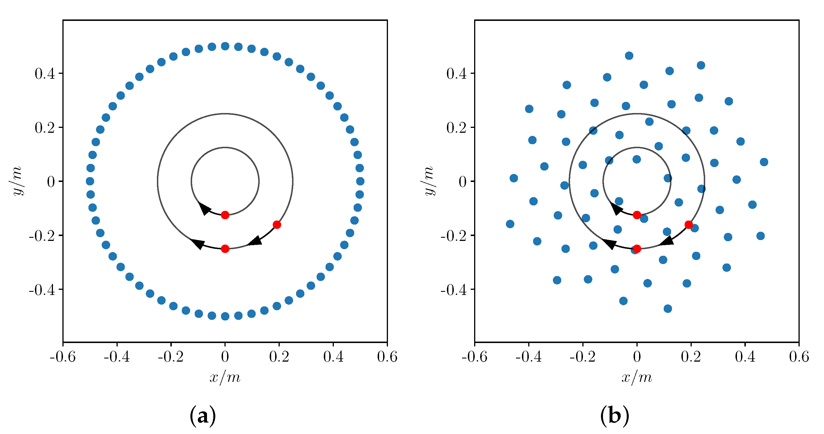
2.2. Virtual Rotating Array
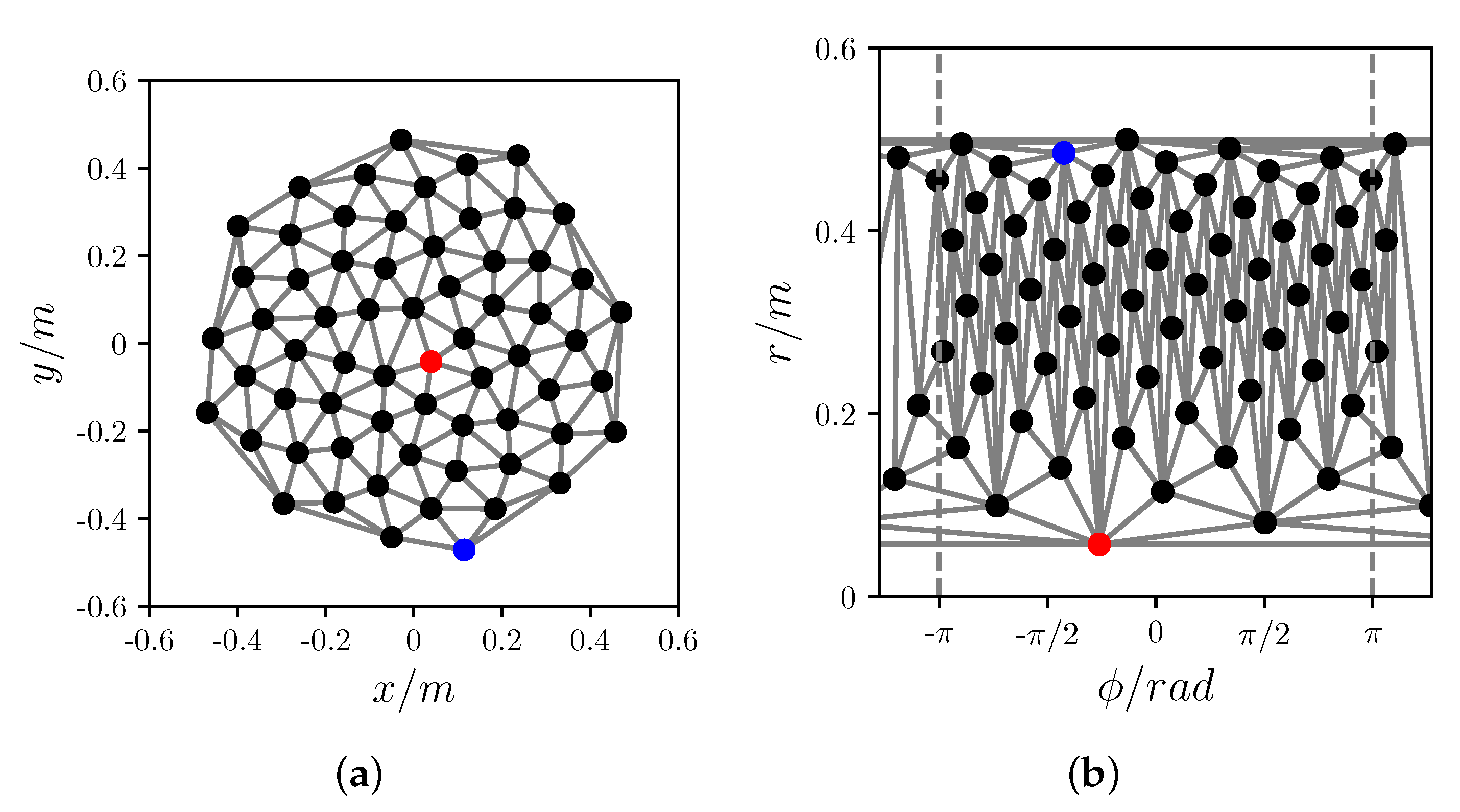
2.3. Mesh Based Triangulation
2.4. Radial Basis Functions
3. Simulation
3.1. Setup
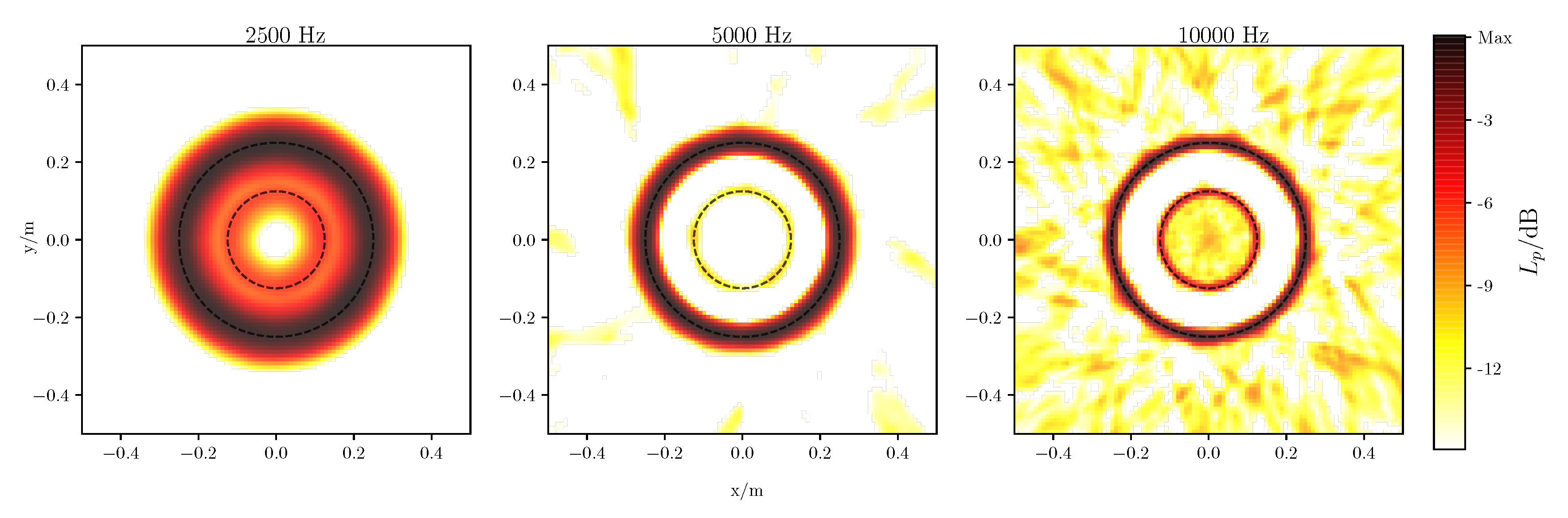
3.2. Results
3.3. Computation Time
4. Experimental Validation
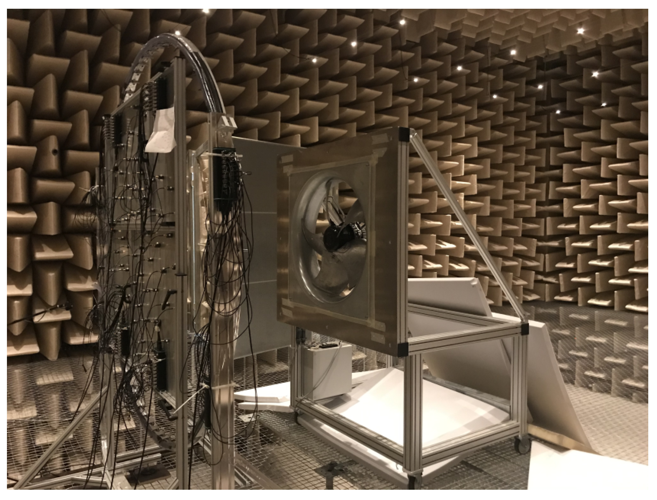
4.1. Setup
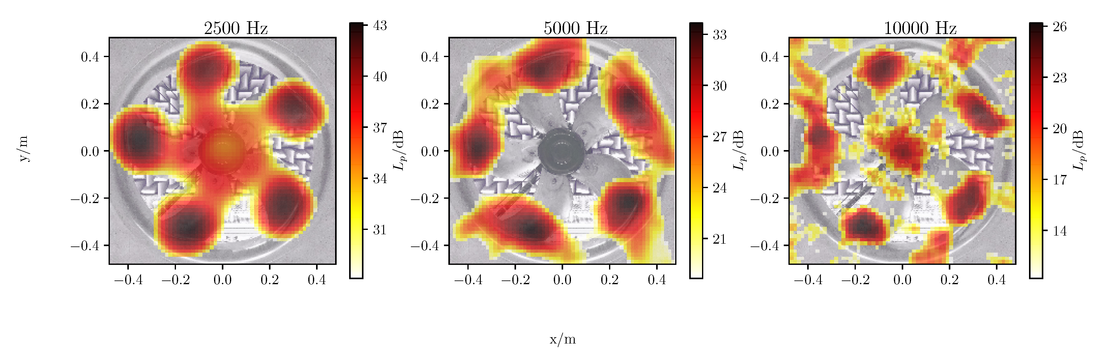
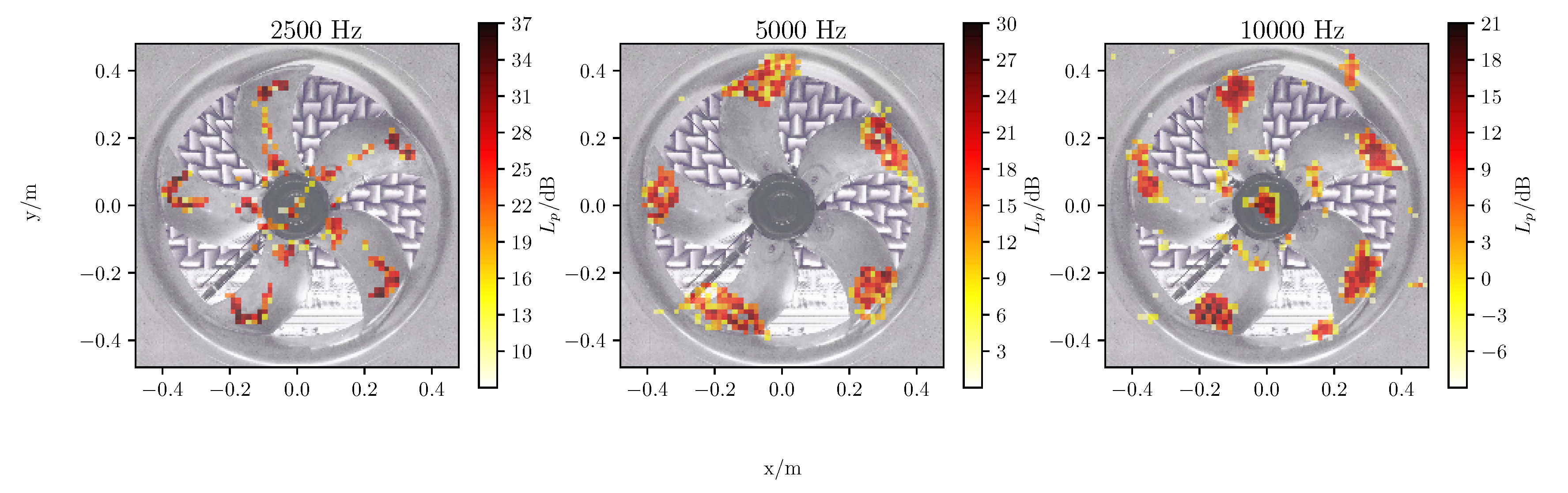
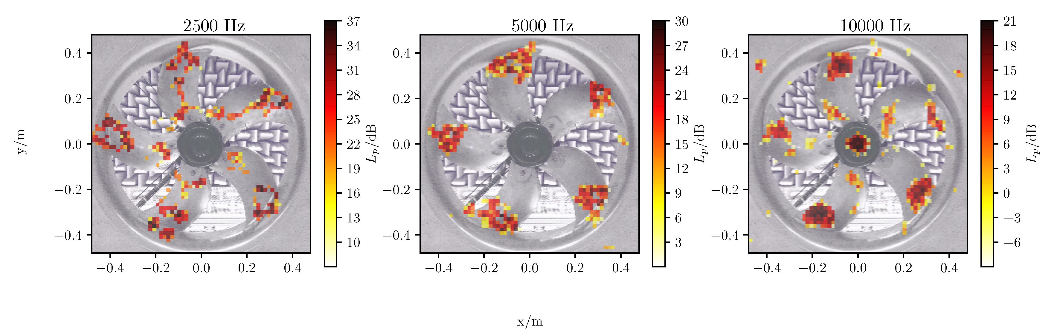
4.2. Results
5. Summary
Author Contributions
Acknowledgments
Conflicts of Interest
Abbreviations
| ROSI | Rotating Source Identifier |
| MD | modal decomposition |
| VRA | virtual rotating array |
| DAMAS | Deconvolution Approach for the Mapping of Acoustic Sources |
| NNLS | non negative least squares |
| RBF | radial basis function |
References
- Sijtsma, P.; Oerlemans, S.; Holthusen, H. Location of rotating sources by phased array measurements. In Proceedings of the 7th AIAA/CEAS Aeroacoustics Conference and Exhibit, Maastricht, The Netherlands, 28–30 May 2001. [Google Scholar] [CrossRef]
- Gomes, J. Noise Source Identification with Blade Tracking on a Wind Turbine. Internoise 2012, 2012, 5115–5126. [Google Scholar]
- Zhang, X.; Chu, Z.; Yang, Y.; Zhao, S.; Yang, Y. An Alternative Hybrid Time-Frequency Domain Approach Based on Fast Iterative Shrinkage-Thresholding Algorithm for Rotating Acoustic Source Identification. IEEE Access 2019, 7, 59797–59805. [Google Scholar] [CrossRef]
- Debrouwere, M.; Angland, D. Airy pattern approximation of a phased microphone array response to a rotating point source. J. Acoust. Soc. Am. 2017, 141, 1009–1018. [Google Scholar] [CrossRef] [PubMed]
- Dougherty, R.P.; Walker, B. Virtual Rotating Microphone Imaging of Broadband Fan Noise. In Proceedings of the 15th AIAA/CEAS Aeroacoustics Conference, Miami, FL, USA, 11–13 May 2009. [Google Scholar]
- Lowis, C.; Joseph, P. Determining the strength of rotating broadband sources in ducts by inverse methods. J. Sound Vib. 2006, 295, 614–632. [Google Scholar] [CrossRef]
- Pannert, W.; Maier, C. Rotating beamforming - Motion-compensation in the frequency domain and application of high-resolution beamforming algorithms. J. Sound Vib. 2014, 333, 1899–1912. [Google Scholar] [CrossRef]
- Herold, G.; Sarradj, E. Microphone array method for the characterization of rotating sound sources in axial fans. Noise Control. Eng. J. 2015, 63, 546–551. [Google Scholar] [CrossRef]
- Kotán, G.; Tóth, B.; Vad, J. Comparison of the rotating source identifier and the virtual rotating array method. Period. Polytech. Mech. Eng. 2018, 62, 261–268. [Google Scholar] [CrossRef]
- Wei, M.; Huan, B.; Zhang, C.; Liu, X. Beamforming of Phased Microphone Array for Rotating. J. Sound Vib. 2019, 467. [Google Scholar] [CrossRef]
- Herold, G.; Ocker, C.; Sarradj, E.; Pannert, W. A comparison of microphone array methods for the characterization of rotating sound sources. In Proceedings of the 7th Berlin Beamforming Conference, Berlin, Germany, 5–6 March 2018; pp. 1–12. [Google Scholar]
- Tóth, B.; Kalmár-Nagy, T.; Vad, J. Rotating beamforming with uneven microphone placements. In Proceedings of the 7th Berlin Beamforming Conference, Berlin, Germany, 5–6 March 2018; pp. 1–13. [Google Scholar]
- Sarradj, E. Three-dimensional acoustic source mapping with different beamforming steering vector formulations. Adv. Acoust. Vib. 2012. [Google Scholar] [CrossRef]
- Brooks, T.F.; Humphreys, W.M. A deconvolution approach for the mapping of acoustic sources (DAMAS) determined from phased microphone arrays. J. Sound Vib. 2006, 294, 856–879. [Google Scholar] [CrossRef]
- Lawson, C.L. Solving Least Squares Problems, 1974th ed.; SIAM: Philadelphia, PA, USA, 1995. [Google Scholar]
- Delaunay, B. Sur la sphère vide. Cl. Des Sci. Math. 1934, 6, 793–800. [Google Scholar]
- Barber, C.B.; Dobkin, D.P.; Huhdanpaa, H. The Quickhull Algorithm for Convex Hulls. ACM Trans. Math. Softw. 1996, 22, 469–483. [Google Scholar] [CrossRef]
- Vogel, H. A Better Way to Construct the Sunflower. Math. Biosci. 1979, 44, 179–189. [Google Scholar] [CrossRef]
- Sarradj, E. A Generic Approach To Synthesize Optimal Array Microphone Arrangements. In Proceedings of the 6th Berlin Beamforming Conference, Berlin, Germany, 29 February–1 March 2016; pp. 1–12. [Google Scholar]
- Buhmann, M.D. Radial Basis Functions: Theory and Implementations; Cambridge University Press: Cambridge, UK, 2003; Volume 12. [Google Scholar]
- Sarradj, E.; Herold, G.; Sijtsma, P.; Merino Martinez, R.; Geyer, T.F.; Bahr, C.J.; Porteous, R.; Moreau, D.; Doolan, C.J. A Microphone Array Method Benchmarking Exercise using Synthesized Input Data. In Proceedings of the 23rd AIAA/CEAS Aeroacoustics Conference, Denver, CO, USA, 5–9 June 2017. [Google Scholar] [CrossRef]
- Herold, G. Microphone Array Benchmark b11: Rotating Point Sources. 2017. Available online: https://depositonce.tu-berlin.de/handle/11303/9404 (accessed on 2 March 2020).
- Johnson, D.H.; Dudgeon, D.E. Array Signal Processing: Concepts and Techniques; P T R Prentice Hall: Upper Saddle River, NJ, USA, 1993. [Google Scholar]
- Sarradj, E.; Herold, G. A Python framework for microphone array data processing. Appl. Acoust. 2017, 116, 50–58. [Google Scholar] [CrossRef]
- Hald, J. Removal of incoherent noise from an averaged cross-spectral matrix. J. Acoust. Soc. Am. 2017, 142, 846–854. [Google Scholar] [CrossRef] [PubMed]
- Zenger, F.J.; Herold, G.; Becker, S.; Sarradj, E. Sound source localization on an axial fan at different operating points. Exp. Fluids 2016, 57, 1–10. [Google Scholar] [CrossRef]
- Herold, G.; Zenger, F.; Sarradj, E. Influence of blade skew on axial fan component noise. Int. J. Aeroacoustics 2017, 16, 418–430. [Google Scholar] [CrossRef]


| Multiquadric | |
| Inverse | |
| Gaussian | |
| Cubic | |
| Thin plate |
| Number of microphones | 64 |
| Array aperture | 1 m |
| Sampling rate | 48 kHz |
| FFT block size | 1024 |
| FFT window/overlap | von Hann/ |
| Focus grid distance | m |
| Focus grid resolution | m |
| Focus grid area | m × m |
| Triangulation, Spiral | RBF, Spiral | Linear, Ring | |||||||
|---|---|---|---|---|---|---|---|---|---|
| Frequency | 2500 Hz | 5000 Hz | 10,000 Hz | 2500 Hz | 5000 Hz | 10,000 Hz | 2500 Hz | 5000 Hz | 10,000 Hz |
| Beam width | 0.125 m | 0.078 m | 0.055 m | 0.129 m | 0.085 m | 0.058 m | 0.071 m | 0.033 m | 0.019 m |
| Dynamic | 19.95 dB | 12.64 dB | 9.71 dB | 14.45 dB | 10.12 dB | 9.67 dB | 9.53 dB | 8.81 dB | 6.18 dB |
| Number of microphones | 63 |
| Spiral array aperture | m |
| Sampling rate | kHz |
| FFT block size | 1024 |
| FFT window/overlap | von Hann/ |
| Focus grid distance | m |
| Focus grid points | 61 × 61 |
© 2020 by the authors. Licensee MDPI, Basel, Switzerland. This article is an open access article distributed under the terms and conditions of the Creative Commons Attribution (CC BY) license (http://creativecommons.org/licenses/by/4.0/).
Share and Cite
Jekosch, S.; Sarradj, E. An Extension of the Virtual Rotating Array Method Using Arbitrary Microphone Configurations for the Localization of Rotating Sound Sources. Acoustics 2020, 2, 330-342. https://doi.org/10.3390/acoustics2020019
Jekosch S, Sarradj E. An Extension of the Virtual Rotating Array Method Using Arbitrary Microphone Configurations for the Localization of Rotating Sound Sources. Acoustics. 2020; 2(2):330-342. https://doi.org/10.3390/acoustics2020019
Chicago/Turabian StyleJekosch, Simon, and Ennes Sarradj. 2020. "An Extension of the Virtual Rotating Array Method Using Arbitrary Microphone Configurations for the Localization of Rotating Sound Sources" Acoustics 2, no. 2: 330-342. https://doi.org/10.3390/acoustics2020019
APA StyleJekosch, S., & Sarradj, E. (2020). An Extension of the Virtual Rotating Array Method Using Arbitrary Microphone Configurations for the Localization of Rotating Sound Sources. Acoustics, 2(2), 330-342. https://doi.org/10.3390/acoustics2020019