1. Introduction
The primary intent of this communication is to illustrate that adaptive signal processing (such as minimum variance distortionless response, or MVDR), converges, without any knowledge, or use, of the linear, inviscid, momentum equation (relating the acoustic pressure gradient to the temporal gradient of acoustic particle velocity), to physics-based optimal solutions (which by necessity invoke the equation of momentum). This is interesting, and useful in that it confirms, at least in ideal spherically isotropic acoustic noise fields with perfectly correlated incident signals, that adaptive processing secures optimal solutions. Directional acoustic sensors, such as acoustic vector sensors and dyadic sensors, are used here to demonstrate the equivalence between adaptive shading coefficients and physics-based shading. This communication does not advocate for any type of adaptive processing over another, instead it is directed at demonstrating equivalence (which requires either that the adaptive scheme form gradients, or, conversely, that the physics-based solution forms the covariance matrix).
Amplitude shading coefficients (similar terms include, simply shading or weights) are commonly implemented in RADAR and SONAR arrays; these coefficients provide a means to manipulate the overall structure of an array’s angular response. Typically, they are used to lower the sidelobe levels of the array’s beam response function in order to improve signal-to-noise ratios (SNRs). Shading coefficients can be real, or complex-valued. Uniform, or unit, coefficients are, by default, equivalent to an unshaded array, with the set of weights being applied to each array element, or along a continuous array aperture, equal to unity. In the past, Dolph–Chebychev [
1,
2,
3] and Taylor [
4] shading was regularly implemented as a means to improve SNRs of acoustic arrays.
Over the past couple of decades, adaptive beamforming (ABF) algorithms [
5] have emerged as an often superior processing technique to generate near-optimal amplitude shading coefficients, providing the right balance between reduced sidelobe levels and mainbeam width.
In this paper, a comparison between ABF-derived shading weights and optimal physics-based weights for directional sensors is presented. If ABF techniques provide optimal solutions, then the two weight sets should be identical.
In order to create a directional sensor, one can proceed in two different ways. The first approach is to use pressure sensors, such as microphones or hydrophones, and combine the measurements from multiple sensors in order to obtain information about the direction of an impinging wave. For example, a typical approach is to take finite differences between adjacent pressure sensors in order to approximate an acoustic dipole. Sonobuoys are often constructed to estimate direction in this manner.
A finite difference approximation to a gradient, however, involves inherent approximation errors. Such gradient approximations are not limited to the first-order; Hines [
6] and D′Spain [
7], using a line array of closely-spaced pressure sensors steered to end fire, examined first, second, and higher order finite differences. With increasing orders of the gradients, the line array becomes more superdirective. There is a simple relationship between the order of the finite difference and directivity [
7,
8,
9]. That is, the first order difference results in an angular response proportional to the cosine of the incident angle (dipole), second order, cosine square, third order, cosine raised to the third, and so on. Here, in total, the array of differenced pressure sensors, in any configuration (linear, planar, volumetric) are referred generally to as arrays of directional sensors.
An alternative approach to creating a directional sensor is direct measurement of additional acoustic quantities. For example, acoustic particle velocity can be directly measured; the velocity is proportional to the gradient of acoustic pressure via the linear momentum of the acoustic pressure field. Such a vector sensor eliminates the need to take a finite difference to estimate the pressure gradient, a first-order quantity. Thus, a particle velocity sensor is an example of a first-order sensor.
This paper shows that, for a perfectly correlated signal in a spherically isotropic noise field, adaptively beamforming a set of discrete pressure sensors generates shading coefficients, or weights, equivalent to those obtained theoretically for the optimal (extrema) beamforming of an acoustic sensor which directly measures acoustic field quantities. The result suggests that adaptive processing algorithms innately seek physics-based solutions; the adaptive weights are equivalent to those formed by optimizing the pressure gradients, obtained from a pre-existing and fundamental physical understanding of the behavior of the acoustic field.
2. Physics-Based Weights for a Directional Sensor
Consider first a single-axis vector sensor, which is restricted for simplicity to measurement of only one component of acoustic particle velocity, say aligned along the vertical
z-axis. The summed beamformed response can be written as:
where the weight set is
,
where
p is the acoustic pressure, and
is an acoustic particle velocity measured along the
z-axis. The weight
is used to absorb the conversion from pressure to velocity, that is, the arbitrary weight is taken to be divided by the acoustic impedance of the fluid,
, so that the units are consistent in Equation (1).
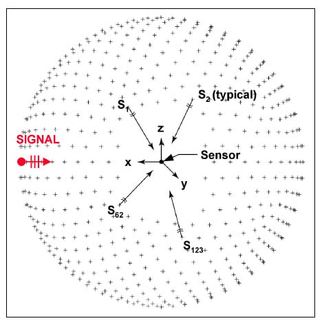
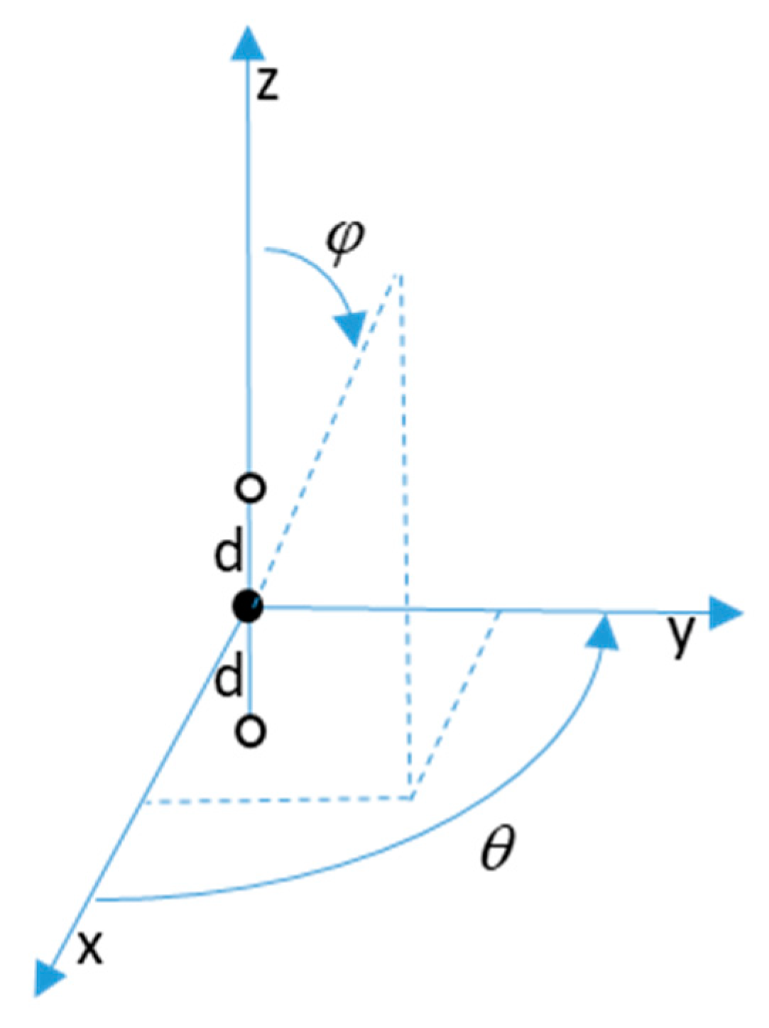
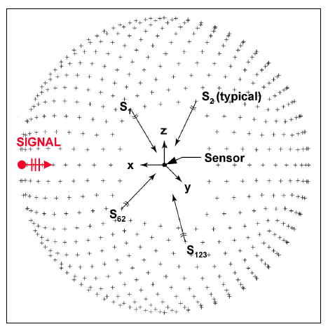
Figure 1 illustrates the sensor configurations. The solid circle at the origin represents either a single acoustic pressure sensor, or a single directional sensor which measurements additional quantities of the acoustic field, such as acoustic particle motion. The two open circles represent adjacent pressure sensors, which can be used to measure acoustic pressure gradients.
The configuration along the vertical axis simplifies the derivation below of optimal directivity; the response becomes symmetric in azimuth angle, , and dependent only upon elevation angle, . In Equation (1), and mostly throughout, we assume a harmonic time dependence which is ignored.
Alternatively, for an impinging time-harmonic plane wave, the beamformed response can be written in terms of the pressure field. In the time domain, we take the impinging harmonic acoustic wave, measured on the
z-axis, to be:
where
and
. Here
denotes the polar angle of incidence of a plane wave impinging on the sensor. In the frequency domain, the first two pressure gradients are:
For any order, the general formula is . Note the proportional scaling of the directional cosine, , by the known constant . To weight and sum (that is, beamform) these gradients with acoustic pressure, either the acoustic pressure must be converted to a corresponding planewave velocity amplitude (as was done above in Equation (1)). Alternatively, the velocity amplitude may be converted to a corresponding planewave pressure amplitude. Both types of conversions are used here for convenience and to simplify derivations.
If the goal is to rewrite the beam response solely in terms of pressure, then the pressure gradients (Equations (3) and (4)) can simply be converted into pressure by multiplying each gradient by and then absorbing this scaling factor into the shading coefficients. This scaling simplifies the optimal directivity calculations. The scaling, or weight conversion, used is different than that used in Equation (1), with because what is assumed now to be measured are pressure gradients rather than, for example, a direct measurement of particle velocity (particle velocity would be calculated from the approximated pressure gradients).
In terms of acoustic pressure, the beam response for any order directional sensor aligned along the
z-axis is:
For first and second order directional sensors, Equation (5) becomes:
and
where
,
and
have absorbed (were divided by),
and
respectively. The units of Equations (6) and (7) thus differ from that of Equation (1).
Optimality of weights is determined by optimality of the associated directivity of the sensor. Directivity is defined as a ratio of signal-to-noise ratios, that is, the SNR of an omni-directional sensor, relative to the SNR of a directional sensor (or array of sensors), in a spherically isotropic acoustic noise field. The directivity factor, for a signal arriving directly down the boresight of the
z-axis, and any order sensor can be shown [
9,
10] to be:
For a single omni-directional sensor, n = m = 0, and as expected, The directivity index is defined as .
2.1. Physics-Based Optimal Weights for a First-Order Directional Vector Sensor
For a first order single axis directional sensor (6), normalized so that
at a given look direction,
, the directivity factor (8) is:
where
is the response at steered elevation angle,
. The optimal weight for the particle velocity component, which maximizes directivity, is obtained by solving for the extrema in Equation (9). Setting
and solving, we obtain
. Thus, when steered to endfire, the optimal weight pair for this simple single axis directional sensor is
. This corresponds to a directivity index of 6 dB.
The particle velocity shown in Equation (1) can be identically recast, via linearized momentum, in terms of a gradient of pressure, that is:
which is the same expression as Equation (6) with
and
, so as before the optimal weights are
and the directivity index is 6 dB.
Equation (10) explicitly includes the pressure gradient. Hence, the beam response,
, in Equation (10) can now be approximated using a two-point finite difference,
that is
where
and
wa1 and
wa2 are the corresponding weights multiplying the two separated pressure sensors. Substituting the physics-based optimal weights,
and chosen parameter values
,
and
we find that:
Below we will compare these values to those obtained using the adaptive MVDR approach.
2.2. Physics-Based Optimal Weights for a Second-Order Directional Dyadic Sensor
The beam response for a single-axis dyadic acoustic sensor, obtained in a manner similar to Equation (10), is:
The same procedure to obtain optimal directivity is employed, though now there are two simultaneous equations to solve for directivity factor extrema (Equation (8)), that is,
and
. Details have been previously derived [
9], and will not be reevaluated here. The optimal physics-based weights, which produce maximum directivity, from [
9], at any steered incident angle becomes:
When again steered to end fire, the optimal weight set for this simple single axis dyadic second-order sensor becomes
(if Equation (13) was rewritten in terms of acoustic particle velocity, and the gradient of velocity, or as in Equation (7), then again the optimal weight set,
, would be the same). Note from Equation (14) that these weights are angular dependent, the maximum occurs at endfire, all other signal arrival angles reduce directivity. It is noted that comparisons between physics-based weights and adaptive weights, for general angles of arrival are not presented. The angular dependency of analytical weights for vector and dyadic sensors are known [
9,
10], though a comparison to ABF weights at oblique incident angles is beyond the scope of this communication, and not likely change the comparison.
As previously done for a vector sensor, we use finite difference approximations to approximate the beam response of a dyadic sensor. Now both two-point and three-point (second order) finite difference approximations are needed. With three closely-spaced pressure sensors
, aligned collinearly along the z-axis, and separated by distance
d, and with
p0 at midpoint, the beam response (Equation (13)) is rewritten as:
With optimal weights
and parameter values
,
and
we obtain:
Below we will compare these values to those obtained from the MVDR approach.
3. Adaptive (MVDR) Weights for a Sensor Array
One adaptive approach is that of the minimum variance distortionless response (MVDR) [
5]. The MVDR approach is to choose the weight set to have minimal response to spherically isotropic noise in the desired look direction
, that is, to solve:
where
denotes the array manifold (see examples below) and the isotropic noise cross-spectral density matrix elements are given by
. Note that this expression, for element-to-element correlations in a spherical isotropic noise field, was theoretically derived in [
11]. This approach does not impose any physics-based knowledge of the acoustic field on adaptive weighting, other than the field is known to consist of acoustic planewaves.
Alternatively, a high resolution Monte Carlo simulation could be generated which would then converge to identical correlations. From Equation (17), the standard adaptive MVDR beamformer solution for the optimal shading coefficient is thus given by:
3.1. Adaptive (MVDR) Weights for a First-Order Directional Vector Sensor
A two-element array, with the pressure sensing elements aligned along the vertical z-axis and separated by a distance,
d, (as denoted by the open circles in
Figure 1), the adaptive beam weights,
would produce an adaptive beam response;
where the two element array manifold has the form
for a monochromatic signal with acoustic wavenumber,
, impinging from direction
. Plugging in the same parameters as in
Section 2, with some manipulation, we obtain:
This weight set identically matches the corresponding physics-based weight set (Equation (12)).
Bear in mind that the adaptive minimum variance distortionless response (MVDR) processor essentially consists of a set of correlation measurements between a collection of pressure sensors and known, or prescribed, signal manifold constraints. The processor has no inherent knowledge of an acoustic field or continuity or acoustic particle momentum, it seeks only to solve for the filter weight vector that minimizes the output noise variance subject to the constraint that the signal is passed through the beamformer without any distortion, that is, where is the steering vector (here s = (cos ) and is the noise covariance matrix for the pressure and particle velocity channels.
Though the equivalence between the two weight sets is not unexpected, given that the solution for optimal directivity is unique, it is interesting that the adaptive processor essentially knows to form the gradient between the two adjacent pressure sensors.
3.2. Adaptive (MVDR) Weights for a Second-Order Directional Dyadic Sensor
Now consider the case of a three-element array,
where the pressure sensing elements are again aligned along the vertical
z-axis and each separated by distance
d (not shown in
Figure 1). Similarly, we have the adaptive beam response:
and array manifold;
where the middle sensor location has now been used as the signal arrival time reference (that is, the center sensor is used to reference the time delays to the two outer sensors). Following the same methodology and parameters as for the two-element array, when the look direction is steered towards end fire, the optimum filter weights become:
after manipulation. The adaptive set, for the dyadic sensor, is again nearly identical to the previously derived physics-based weight set. The slight differences are presumably due to finite difference approximation errors. As the separation distance,
d, varied, the resultant adaptive weights slightly changed. Here, the separation distance was
. Notice, that if the adaptive weights are further approximated as
the beam output can be rewritten simply as
, which immediately is interpreted as the second order finite difference gradient.
For reference,
Table 1 below summarizes the directivity indices (at end fire), using both weight sets, for the vector and dyadic directional sensors.
4. Conclusions
The linearized momentum equation, as all acousticians know, is invoked in the derivation of the acoustic wave equation. Momentum relates, within an inviscid fluid medium, acoustic particle velocity to the spatial gradient of acoustic pressure. As shown here, physics-based derivations explicitly use linear momentum to obtain optimal amplitude shading coefficients. What is also illustrated here, is that adaptive processors, such as MVDR, implicitly form these spatial pressure gradients, as a directional sensor explicitly does, to obtain optimal shading coefficients. Equivalence between adaptive and physics-based weight sets, for both first and second order directional sensors, has been shown. This is a pleasing result; it confirms the merits of adaptive processors, and lends confidence that, for non-isotropic noise fields, adaptive methods will yield optimal solutions. The intent of this communication was not to propose one adaptive technique over another, instead it demonstrated equivalence between physics-based and adaptive processing.
Comparison between adaptively derived shading weights, to those obtained theoretically, can be made with even higher order directional sensors. However, the solution space quickly becomes unwieldy Additional comparisons have been made where the separation distance, d, between the pairs of pressure sensors converged. This, therefore, modified the accuracy of the finite difference approximations, resulting in an expected improvement in the agreement between adaptive and physics-based weights. No comparisons were made here for acoustic planewave signals arriving at oblique angles of incidence. Given that, for a spherically isotropic noise field and a perfectly correlated incident signal, both physic-based and MVDR weights independently generate dipole angular responses, it is taken that oblique angle weights will again be equivalent.

