Applicability of Acoustic Concentration Measurements in Suspensions of Artificial and Natural Sediments Using an Acoustic Doppler Velocimeter

Abstract

For the investigation of turbulence and particles, interaction measurement systems are required, which are able to measure velocity and concentration fluctuations simultaneously. Acoustic Doppler Velocimeters (ADV) are widely used for velocity and turbulence measurements in natural and artificial flows. Based on the acoustic sonar theory, a model is presented that correlates the ADV’s Signal-to-Noise Ratio (SNR) and the suspended solids concentration of several natural (Ems Estuary, Lake Eixendorf, Lake Altmühl) and artificial sediments (Chinafill, quartz powder, bentonite, metakaolin) for the range 0.001 g/L–50 g/L. Within the presented method, the sound absorption in water and on particles is considered in a continuous approach for sampling frequencies up to 100 Hz. The widely-used log-linear relation between the SNR and the concentration, which is only valid for low concentrations, was extended for the high concentration regime. Measurement results show a similar behavior of the SNR with respect to varying suspended solid concentrations for different sediments. However, the analysis of the fit parameters shows systematic differences depending on the type of sediment. It is concluded that the proposed model is applicable as well for laboratory use as for measurements in rivers and estuaries. Finally, we discuss the reliability of the results and the methodology with regard to measurements in rivers, lakes, and estuaries.

1. Introduction

ADV probes provide the opportunity to measure in situ the three-dimensional flow velocity in liquids with a high temporal resolution (up to 200 Hz). This allows evaluating the velocity fluctuations in terms of the turbulent behavior in the flow. The three-dimensional velocity fluctuations $u_i^{\prime }=u_i-{\overline{u}}_i$ are described as the deviation of the mean value ${\overline{u}}_i$. The intensity of turbulence is described by the turbulent kinetic energy k = $\frac{1}{2}\left(\overline{u_i^{\prime }{u}_i^{\prime }}\right)$, which consists of the diagonal contributions of the Reynolds stress tensor, e.g., [1].

Especially in natural surface waters like rivers, channels, lakes, and estuaries, near-bottom suspended solids of different concentrations are common. For instance, in the Ems Estuary in the German Bight, Suspended Solid Concentrations (SSC) were measured up to 300 g/L [2]. Cellino demonstrated that SSC influence the flow behavior within a stream, in particular the vertical structure of turbulence. It was shown that SSC can lead to turbulence damping and decreasing eddy viscosity [3].

The common method to describe the interaction between concentration and turbulence is to quantify the turbulent Schmidt-number Sc${}_t=\frac{{\nu }_t}{K_t}$ with ${\nu }_t$ being the turbulent viscosity and $K_t$ being the turbulent diffusivity. The physical behavior of both quantities is the same, as the diffusivity of particles increases with turbulence. The turbulent Schmidt-number is often used for calibrating experimental and numerical data. Depending on the type of particles, it is given as Sc${}_t$ = 0.3–1.5 [4].

Applying the eddy viscosity hypothesis, ${\nu }_t$ can be formulated by means of the extra diagonals of the Reynolds stress tensor $\overline{u^{\prime }{w}^{\prime }}$ and the vertical gradient of the mean velocity $\frac{\partial \overline{u}}{\partial z}$ in the main stream direction:

$$\overline{u^{\prime }{w}^{\prime }}=-{\nu }_t\frac{\partial \overline{u}}{\partial z}$$

(1)

Following the same principle, $K_t$ is described by the fluctuations of the concentration c${}^{\prime }$ and the vertical gradient of the mean concentration.

$$\overline{c^{\prime }{w}^{\prime }}=-K_t\frac{\partial \overline{c}}{\partial z}$$

(2)

In order to investigate the interaction of turbulence and particle concentration, it is necessary to measure the velocity and the concentration fluctuations simultaneously. Further, to detect as many turbulent eddies as possible, the measuring frequency should be as high as possible.

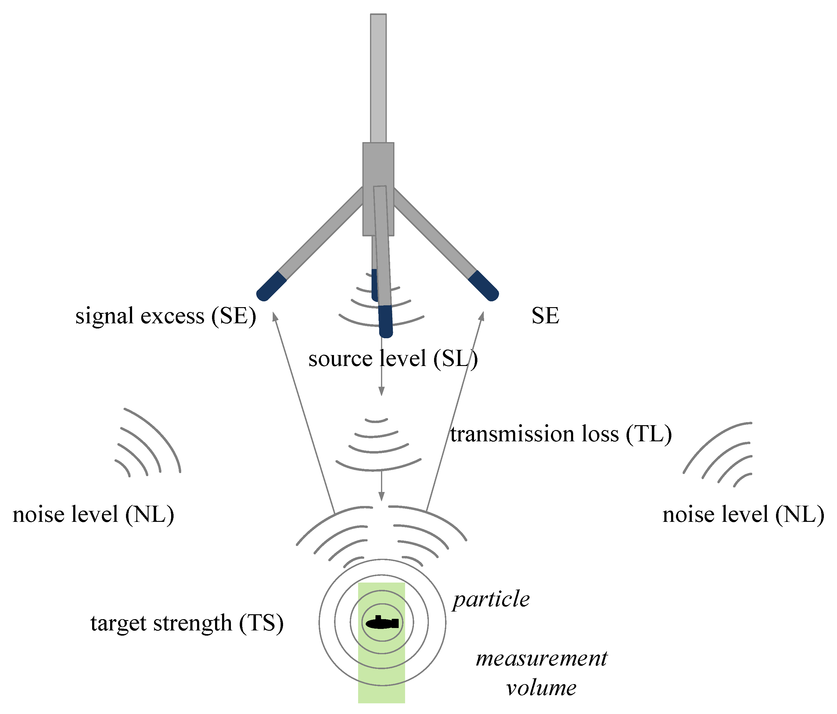
Salehi et al. summarized three methods for measuring the particle concentrations in currents [5]: (1) the extraction of samples at different positions with a suction device and the external analysis of the samples taken; (2) determination of the particle concentration through scattering and reflection of light (OBS); and (3) the concentration measurement by means of the reflection and scattering of an acoustic signal. The intensity of sound is attenuated by the particles within the measurement volume. Furthermore, the reflected signal is superimposed by noise, which is taken into account by the Signal-to-Noise Ratio (SNR).

As mentioned in Equation (2), for the investigation of the diffusivity coefficient $K_t$, measurements of the concentration fluctuations are necessary. Applying the suction method, for instance, no information about the concentration and velocity fluctuations at the same time and location are obtained. Optical measurement devices provide a wide spectrum of recordable concentrations; however, they are not able to measure the velocity. The investigations of Fugate et al. show higher accuracy for SSC measurements in estuaries when using acoustic devices rather than optical instruments [6]. Acoustic devices, like ADV probes, are used to measure the three-dimensional flow velocities with a sampling frequency f up to 200 Hz. Additionally, the SNR is recorded, which is affected by the particle concentration in the measurement volume. If it is possible to find a unique function for the SNR with respect to the concentration, then it is possible to measure velocity, turbulence, and concentration synchronously.

The foundation of the acoustic method is the sonar theory, which was first applied for small particles by Urick in 1948 [7]. Urick investigated the absorption behavior of kaolin and fine silt while using a quartz crystal to send acoustic pulses. After ADV measurements became a standard technique for velocity measurements, the acoustic scattering theory again was applied for concentration measurements [8]. Thorne et al. gave a summary of the advantages of acoustic methods for concentration measurements since optical devices reached their working range at this time [9]. Jay et al. described difficulties when calibrating the SNR for natural rivers, since the reflected signal was strongly dependent on the particle’s material, shape, and size [10]. Hoitink et al. were able to calibrate the SNR for concentrations up to 1 g/L [11]. However, neither study, from Jay et al. and Hoitink et al., considered the sound absorption on particles; that is why their methods are only valid up to approximately 1 g/L.

The acoustic method for concentration measurement can be applied at laboratory conditions with a homogeneous particle distribution and known sediment properties. Ha et al. and Salehi et al. presented laboratory experiments for calibrating the reflected signal intensity and the particle concentration [5,12]. Nevertheless, they neglected the sound attenuation on particles, although it is a crucial parameter. Decrop et al. presented an experimental setup to measure concentrations up to 10 g/L with an ADV probe while considering sound attenuation on particles. Their measurements were conducted with a measurement frequency of 25 Hz [13]. To investigate the interaction of turbulent concentration and velocity fluctuations, higher sampling frequencies are required to resolve turbulent flow behavior.

In order to investigate the interaction of turbulence and concentration, different experimental studies were realized. Best et al. conducted a laboratory experiment to measure velocities and concentrations with a Laser Doppler Anemometer (LDA). However, the application of their optical method was restricted to low concentrations [14]. Cellino used a self-constructed acoustic particle flux profiler for measuring the concentration and velocity with a frequency of 16 Hz [15]. A part of his research was to investigate the decay of turbulence with increasing suspended sediment concentration in a laboratory flume [3].

Moreover, Hurther et al. showed the development of an Acoustic Concentration and Velocity Profiler (ACVP), which was able to measure the two-dimensional velocity field and the concentration over a vertical profile of 25 cm [16]. This device was applied by Revil-Baudard et al. for laboratory experiments on investigations of sheet-flow processes [17]. They reported about maximum concentration measurement frequencies of 4.9 Hz.

The necessity of simultaneously measuring flow velocity and concentration is presented by means of the Ems Estuary (Germany, North Sea) as an example. In the Ems Estuary, simultaneous measurements of flow velocity and concentration are needed in order to describe the dynamics of fluid mud layers. Fluid mud is a high concentrated mud suspension, which has huge impacts on the maintenance of rivers and estuaries, since navigation can be impeded [18]. Recently, Becker et al. showed concentration and velocity measurements of the fluid mud layers in the Ems Estuary and highlighted the unsteady and complex behavior of the mud layers with tide. Within this measurement campaign, velocity and concentration were measured by different devices. Furthermore, no turbulence measurements were presented [19]. Having a measurement device that would be able to measure velocity, concentration, and turbulence simultaneously, the unsteady dynamics of such fluid mud layers could be investigated in more detail.

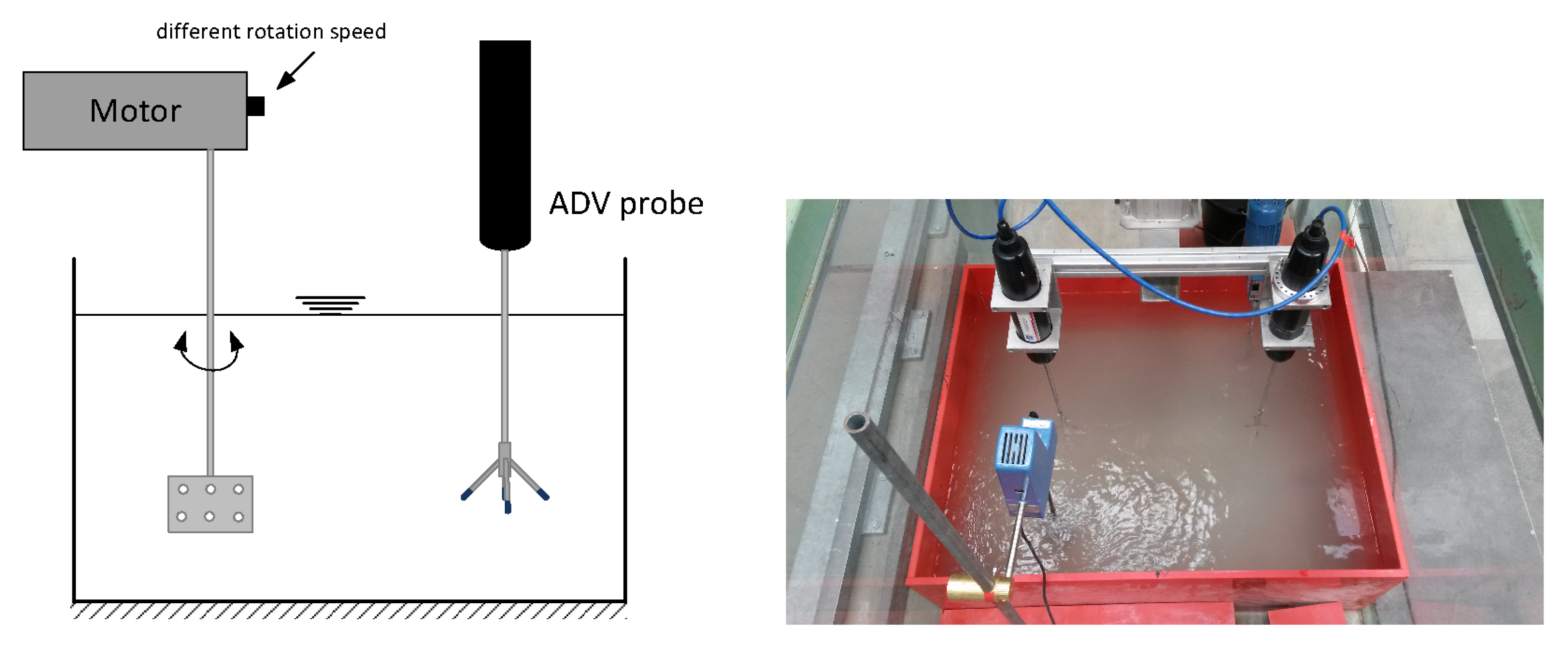
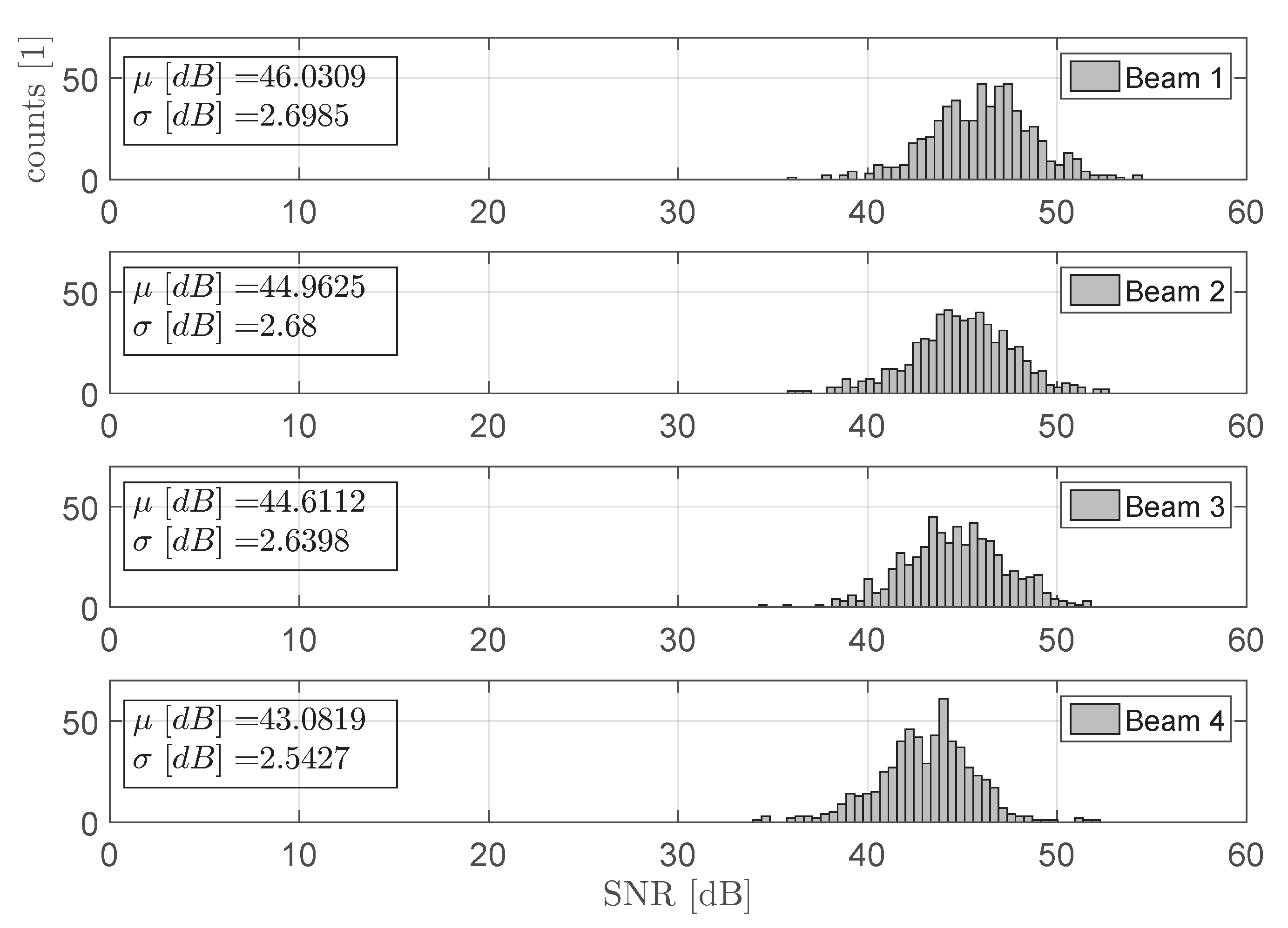
With developing measuring techniques, more accurate turbulence results are expected when using measurement devices with sampling frequencies as high as possible. In this case, small eddies are able to be resolved, which could not be recognized from the measurement device in former studies. Therefore, a Vectrino Profiler (Nortek, Norway) was used with a sampling frequency of 100 Hz. The Nortek Vectrino Profiler was launched in 2010 and consists of a single central transceiver and four passive receivers at an angle of 30${}^{\circ }$ towards the transceiver. A detailed description of the probe was given by Craig et al. and by Thomas et al. [20,21].

Within this paper, a method is presented to model the concentration of different suspended materials by means of the SNR with a modern ADV probe (Vectrino Profiler). The acoustic model is based on the well-known sonar theory approach, and it is applied for artificial and natural river sediments. The authors show how sound attenuation is considered in water and on sediment particles within the sonar theory-based model. In experimental studies for cohesive sediment dynamics, quartz powder, metakaolin, and Chinafill are often used [13,22,23]. Therefore, the following artificial sediments were investigated: quartz powder, bentonite, metakaolin, and Chinafill. Afterwards, the results were compared with those of natural sediments from the Ems Estuary on the German Coast, Lake Altmühl, and Lake Eixendorf, both located in Bavaria, Germany. The experimental setup and the proceeding measurements are presented. Furthermore, the authors describe the analysis of the results of different sediments in order to specify the model’s applicability in nature. Furthermore, it is shown that concentrations can be measured up to 50 g/L depending on the type of sediment.

This paper describes a method for simultaneously measuring velocity, turbulence, and concentration, which can be applied in laboratory investigations, as well as in rivers, estuaries, or lakes. The characteristics of the method are presented in detail, and indications are given for practical use in nature. The results of this study provide a contribution for further investigations of turbulence and diffusivity equally in the laboratory and for use in nature.

2. Acoustics of the ADV Probe

In the following, the theoretical aspects are described for sound and particles’ interaction in water. First, the particle diameters are verified, which are applicable to the acoustic backscatter theory. Afterwards, the authors present the implementation of the general sonar theory using the backscatter intensity. The aim of this part is to derive an equation to relate the suspension concentration to an acoustic quantity, which can be measured by the ADV probe.

2.1. Rayleigh Scattering and the Intensity of the Backscatter Signal

The working principle of ADV devices is based on Rayleigh scattering, which occurs when the diameter of the particle is smaller than the wavelength of the emitted signal. In that case, the energy transfer towards the particle can be neglected. For Rayleigh scattering, the condition:

$$k_{w}r<1$$

(3)

has to be fulfilled, with $k_w$ = $\frac{2\pi }{\lambda }$ as the wave number, $\lambda$ as the wavelength, and r as the particle radius [24]. Decrop et al. argued that a sufficiently high backscatter intensity only can be achieved for $k_{w}r$ > 0.05 [13].

In this study, we used different sediments with mean particle diameters 7 $\mathsf{\mu }$m ≤ $d_{50}$ ≤ 20 $\mathsf{\mu }$m. The ADV’s emitter frequency was F = 10 MHz, which lead to 0.147 ≤ $k_w$r ≤ 0.419 (

Table 1. The different particle diameters used to investigate the validity of Rayleigh scattering.

Sediment/Location	${\mathit{d}}_{50}$ ($\mathsf{\mu }$m)	${\mathit{k}}_{\mathit{w}}\mathit{r}$$(-)$
Quartz powder	18	0.377
Bentonite	7	0.147
Metakaolin	9	0.189
Chinafill	9	0.189
Ems 2012	10	0.209
Ems 2015	18	0.377
Lake Eixendorf	20	0.419
Lake Altmühl	12	0.251

). Therefore, the condition was fulfilled to apply the principles of Rayleigh scattering here.

The intensity $S_v$ of the backscatter signal increases with the reflecting particle amount $n_b$ inside the measurement volume and their scattering cross-section ${\sigma }_{bs}$. Assuming unidirectional reflection, Medwin and Clay presented the scattering cross-section as:

$${\sigma }_{bs}=4\pi r^6{k}_w^4\mathrm{Y}$$

(4)

The factor $\mathrm{Y}$ is a material parameter, which is determined as:

$$\mathrm{Y}={\left(\frac{\Delta E-1}{3\Delta E}\right)}^2+\frac{1}{3}{\left(\frac{\Delta \rho -1}{2\Delta \rho +1}\right)}^2$$

(5)

where $\Delta \rho ={\rho }_s/{\rho }_w$ is the density ratio of the particle and water and $\Delta E$ = $E_s$/$E_w$ is the elasticity ratio. The backscatter signal can be described in terms of $n_b$ and ${\sigma }_{bs}$ as the volume backscattering coefficient:

$$s_v=n_b{\sigma }_{bs}$$

(6)

which is a measure of the backscatter strength from particles. The backscatter strength increases with the number of reflecting particles and with the size of the scattering cross-section. That means that an increase of $s_v$ is equivalent to a greater backscatter intensity, which is received by the ADV probe. The backscatter strength can be expressed in decibel units as [11,24]:

$$S_v=10lo{g}_{10}\left(n_b{\sigma }_{bs}\right)$$

(7)

Assuming spherical particles with a mass $M=4/3r^3\pi {\rho }_s$, the concentration:

$$C=M{n}_b$$

(8)

can be calculated from the number of particles inside the scattering volume. Combining Equations (4), (6) and (8) leads to:

$$S_v=10lo{g}_{10}\left(\frac{3r^3{k}_w^4\mathrm{Y}}{{\rho }_s}C\right)$$

(9)

which describes the backscatter intensity as a function of the concentration.

The backscatter intensity $S_v$ must not be mistaken with the ADV receiver intensity. $S_v$ is rather the backscatter intensity in the vicinity of the particle. On the way back to the ADV receiver, the signal intensity is exposed to further losses.

2.2. Application of Sonar Theory

The ADV transmitter emits an acoustic signal, which will be reflected on particles in the water, but it is only partly received by the probe’s receiver. This process can be described by the principles of active sonar, which are illustrated in Figure 1. All quantities within the sonar theory are described in dB.

The emitted signal intensity (Signal Level (SL)) is exposed to Transmission Losses (TL) in both traveling directions. Additionally, the reflected signal is influenced by the specifics of the particles (e.g., shape, size, elasticity), which are accounted for in the Target Strength (TS). The ambient sound, which is not related to the ADV probe, is called noise and is described in NL as the noise level. Within sonar theory, SE (Signal Excess) is the received backscatter intensity inclusive of noise. In order to detect the reflected signal, SE has to overcome at least the noise intensity (Noise Level (NL)). The sonar balance equation as presented in similar form in Hoitink et al. and in Salehi et al. reads [5,11]:

$$SE-NL=S_v-40lo{g}_{10}\left(R\right)-2\alpha R+C_{ADV}$$

(10)

$\left(SE-NL\right)$ is the backscatter intensity under exclusion of noise (it is also called the Signal-to-Noise Ratio (SNR)). The target strength within the measurement volume is the backscatter intensity $S_v$. $C_{ADV}$ describes the influence of additional device-specific settings. The transmission losses 2TL = 40 $lo{g}_{10}\left(R\right)$ + 2$\alpha R$ are accounted for in both directions, while R is the distance from the transmitter to the measurement volume [25]. The effect of sound absorption is considered by:

$$\alpha ={\alpha }_w+{\alpha }_p$$

(11)

as the sum of the occurring sound absorption losses in water ${\alpha }_w$ and on particles ${\alpha }_p$.

The ADV device, which is used in the experiment, has an emitter frequency of F = 10 MHz. For this emitter frequency, the coefficient for absorption losses in water is given as ${\alpha }_w$ = 26.9 dB/m [26]. Unfortunately, the particle absorption coefficient ${\alpha }_p$ is not a constant. It depends on the acoustic properties of the transmitted signal and the properties of the particles. Urick presented an approach for the particle absorption coefficient in granular suspensions, which is valid for homogeneous particle distributions [7]. This approach was successfully applied by Hoitink et al. and Salehi et al. when conducting ADCP (Acoustic Doppler Current Profiler) and ADV measurements [5,11]. Therefore, Urick’s formula for ${\alpha }_p$ was used within this paper, while the constant term is called the Urick-coefficient $Ur$ $[{\mathrm{m}}^2/\mathrm{kg}]$. $Ur$ is calculated by sediment and material constants, namely the particle radius r, the solid density ${\rho }_s$, the specific density ratio $\Delta \rho ={\rho }_s/{\rho }_w$, the molecular viscosity ${\nu }_m$, the emitter frequency F, and its wave number $k_w$:

$${\alpha }_p=\underset{Ur}{\underbrace{\left(\frac{k_w^4{r}^3}{96{\rho }_s}+\frac{k_{w}s{\left(\Delta \rho -1\right)}^2}{2{\rho }_s\left(s^2+{\left(\Delta \rho +\delta \right)}^2\right)}\right)\frac{20}{ln\left(10\right)}}}C$$

(12)

The following auxiliary variables are introduced:

$$s=\frac{9}{2\beta r}\left(1+\frac{2}{\beta r}\right)$$

$$\delta =\frac{1}{2}\left(1+\frac{9}{\beta r}\right)$$

$$\beta =\sqrt{\frac{\pi F}{{\nu }_m}}$$

It is highlighted that next to sedimentological and device-specific parameters, Equation (12) is a function of the concentration C.

2.3. How Particles Influence the SNR

The intensity of the backscatter signal, which is received by the ADV, depends on the sediment concentration. Two effects have to be considered simultaneously. First, an increasing particle concentration will be accompanied by an increase of the overall scattering cross-section, if a homogeneous particle distribution is ensured over the volume. This leads to rising SNR values. Second, while ${\alpha }_p$ is a function of the concentration, increasing sound absorption causes a decrease of the SNR.

Combining Equations (9) and (10), splitting 2$\alpha R=$2${\alpha }_{p}R+$2${\alpha }_{w}R$, introducing the transformation parameter ${\Pi }_1$, and solving for the concentration leads to:

$$lo{g}_{10}\left(AC\right)=4lo{g}_{10}\left(R\right)+\frac{1}{10}{\Pi }_{1}SNR-\frac{C_{ADV}}{10}+\frac{1}{5}{\alpha }_{w}R+\frac{2R}{10}{\alpha }_p$$

(13)

with:

$$A=\frac{3r^3{k}_w^4\mathrm{Y}}{{\rho }_s}$$

and:

$${\Pi }_{1}SNR=SE-NL$$

In order to quantify the dependency of the SNR and the concentration, we present an experiment to measure the SNR in suspensions of pre-defined concentrations. Afterwards, the measurements will be compared to the results gained by the sonar theory model.

3. Experimental Investigation

After deriving the relation between the concentration and the SNR, within this section, the authors present the experimental setup for calibrating the SNR to the concentration of suspension flows. After discussing the suitability of the used ADV device, the exemplary results are presented. On behalf of simplicity, the description of the experimental setup is restricted only to one sediment type, namely quartz powder. Results of the resuming sediments are shown in Section 4.

3.1. Experimental Setup

Figure 2 illustrates the experimental setup consisting of a rectangular box, which was $B_1$ = 0.96 m wide and $L_1$ = 0.80 m long. The box was mounted on a steel bottom. The water depth in the box was $H_1$ = 0.30 m. Two opposite installed stirrers guaranteed homogeneously-mixed suspensions. A Nortek Vectrino Profiler ADV probe (sampling frequency f = 100 Hz) was mounted on a dynamometer wagon and adjusted in a way that the probe was box-centered and able to be translated vertically.

Before adding the sediment, an initial reference SNR was measured to account for the prevailing contamination in the water used. The sediment was weighed with a high precision electronic scale in order to prepare the desired concentrations. The concentration was stepwise increased from C = 0.001 g/L–50 g/L. To prevent the aggregation of particles, we initiated a strong turbulence by the stirrers and added the powder through a sieve. To control vertical homogeneous mixing conditions, measurements were conducted at four depths, equally separated.

3.2. Suitability of the ADV Probe

To determine the most unambiguous relation between the SNR and the concentration, firstly, a clear SNR signal was needed, and secondly, the deviations within the four receiver signals had to be as small as possible. Figure 3 shows the box plot evaluation of the SNR signal for three repeated measurements in a low concentrated quartz powder suspension.

The scattering of the Interquartile Range (IQR) was similar for all four beams and for three repetitions, within the range of 2–3 dB. It is noticeable that Beam 4 was measuring lower values than the remaining receivers. On the contrary, Beam 1 was providing slightly greater values.

In the case of Run 03, this behavior is shown in Figure 4, where the SNR signals are presented as histograms. While fitting Gaussian curves to the histograms, the mean $\mu$ and the standard deviation $\sigma$ were calculated. It shows that Beams 2 and 3 provided similar mean values ${\mu }_2$ = 44.96 dB and ${\mu }_3$ = 44.61 dB, which is in between ${\mu }_1$ = 46.03 dB and ${\mu }_4$ = 43.08 dB. Nevertheless, when averaging the data of all four receivers, the equal deviations of Beam 1 and Beam 4 were eliminated. The standard deviations of the SNR distributions were in the range of $\sigma$ = 2.5–2.7 dB, which corresponded to the values obtained by the box plot evaluation.

Due to the narrow range of the IQR and the few detected outliers in the box plots, as well as similar mean values and low standard deviations, it was assumed that this ADV probe was satisfactorily suitable for calibration measurements.

3.3. Acoustic Feedback: Based on Quartz Powder Measurements

After averaging the SNR data of the four receivers, the SNR was plotted against the quartz powder concentration in semi-logarithmic scale. While the SNR of the four receivers was already averaged, Figure 5 illustrates the dependency of SNR on the concentration for two different measurement heights above the bottom ($z_1$ = 19 cm, $z_2$ = 15 cm). Although the measurements at different heights fluctuated in a range of about 5 dB, no systematic deviations related to the z-coordinate were noticeable. Therefore, we concluded that the prepared suspensions were well mixed, and a homogeneous concentration was apparent in the experimental box.

In semi-logarithmic scale, a characteristic linear shape can be observed up to C ≈ 1 g/L. For higher concentrations, no linear dependency can be regarded any more. On the basis of the quartz powder measurements, we propose the following subdivision of the chart in Figure 5 into three acoustically-characteristic regions. (I) The whispering zone: The whispering region is characterized by few echoes returning from the measurement volume due to low particle concentration. Within this region, SNR data reacted sensitively to small deviations of the particle amount. The log-linear behavior between the SNR and the concentration was limited in this region since the ADV probe always detected a minimum SNR value. (II) The audibility zone: Within this region, a clear echo intensity was received. The absorption losses on sediment particles were considered to be low. It is common to neglect ${\alpha }_p$ for concentrations up to C ≈ 1 g/L [5]. (III) The muffling zone: Due to a high concentration, the acoustic backscatter signal was intense. In this region, the log-linear shape provided no suitable data approximation. Still, the overall scattering coefficient was increasing with concentration, which led to an increase of SNR. At the same time absorption, losses on particles were becoming more dominant. This resulted in a vertex after which the SNR decreased again. When absorption losses overcome the increase of the scattering coefficient, SNR data will decrease as a matter of fact.

The continuous flattening of the data points (with increasing concentration) in Figure 5 was due to the increasing influence of ${\alpha }_p$. Not knowing at which concentration ${\alpha }_p$ would be negligible or not, it is proposed to consider both the absorption coefficients ${\alpha }_w$ and ${\alpha }_p$ irrelevant with respect to the concentration. Since ${\alpha }_p$ is a function of C itself (Equation (12)), it will be automatically reduced in the case of low C. Therefore, a steady function SNR = f$\left(C\right)$ has to be found.

4. Modeling the Signal-to-Noise Ratio

In this section, we describe the methodology of fitting the sonar equation parameters (Equation (13)) into the measurements. Doing so, the influence of ${\alpha }_p$ is considered. Furthermore, we show how the sonar model is applied to compute the concentration by means of the SNR. In the end, we evaluate and compare the results of different kinds of sediment.

4.1. Application of the Sonar Equation

When rearranging Equation (13), the SNR is described as:

$$SNR=\frac{10}{{\Pi }_1}\left(lo{g}_{10}\left(AC\right)-4lo{g}_{10}\left(R\right)+\frac{C_{ADV}}{10}-\frac{1}{5}R{\alpha }_w-\frac{2R}{10}{\alpha }_p\right)$$

(14)

with the three unknown parameters: ${\Pi }_1$, ${\alpha }_p$ = ${\Pi }_2$·$U{r}_{analyt.}$·C and $C_{ADV}$. ${\Pi }_2$ is interpreted as an empirical correction factor of $U{r}_{analyt.}$.

Figure 6 describes the experimental data in comparison to the parametrized sonar function, which is based on Equation (14). The parameterization of the sonar equation was done with a non-linear least-squares method in the MATLAB^® Curve-Fitting-Tool. It can be seen that the fit function and the measurements are in good agreement. The unknown parameters were found as ${\Pi }_1$ = 1.712, ${\Pi }_2$ = 4.34, and $C_{ADV}$ = 42.08 dB. We mention that the analytical solution of the Urick-coefficient gave $U{r}_{analyt.}$ = 1.727 m${}^2$/kg, which deviated in comparison to $U{r}_{sonar}$ = ${\Pi }_2$ · $U{r}_{analyt.}$ = 7.43 m${}^2$/kg. Furthermore, we mention that ${\Pi }_1$ is a transformation coefficient of the SNR (see Equation (13)), which is expected to be close to 1.

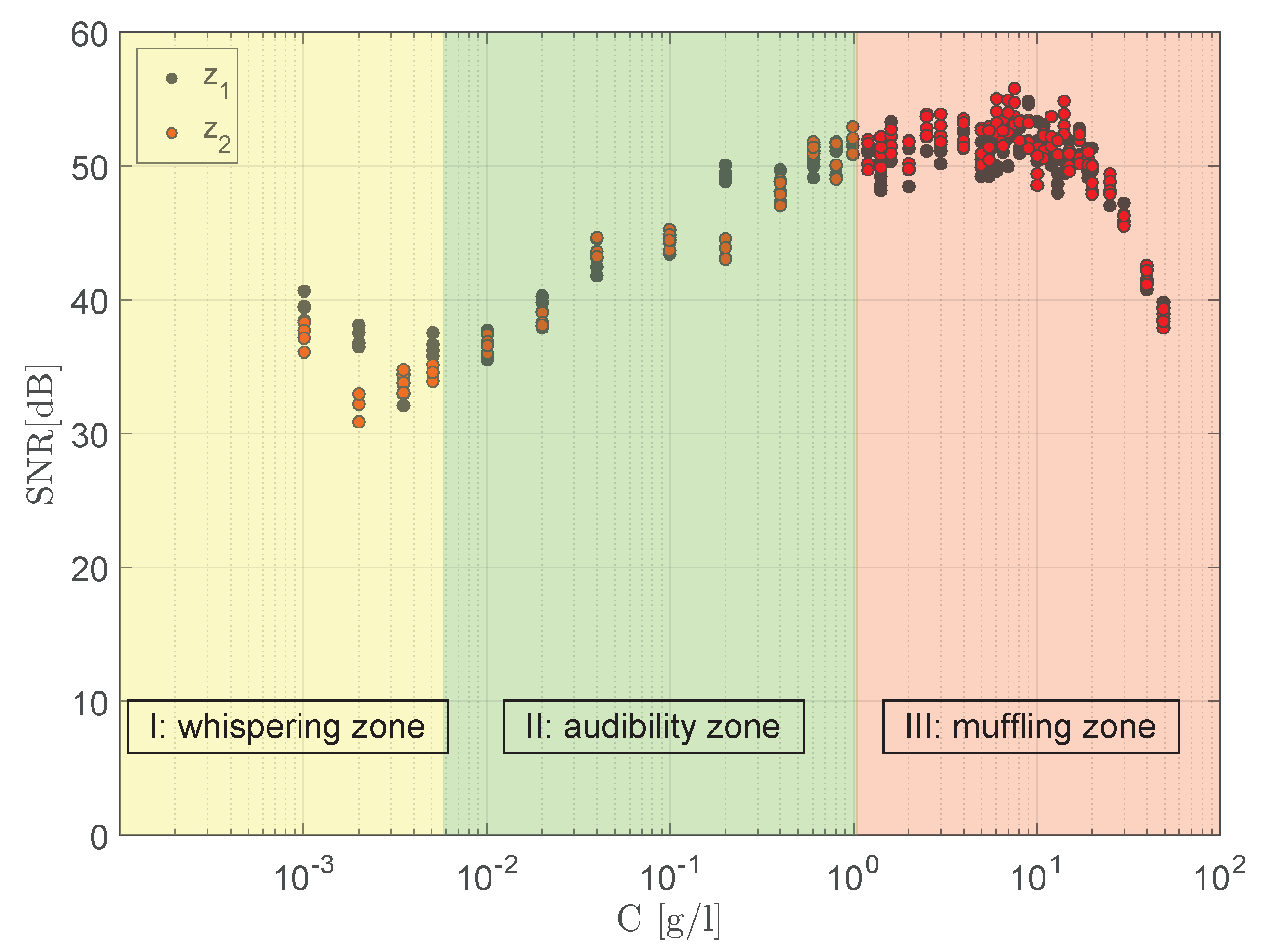
When considering the region of high concentrations, the sonar model describes a flattening followed by a decrease of SNR. This behavior is explained by the absorption coefficient ${\alpha }_p$ in the sonar equation. Even if the influence of ${\alpha }_p$ remains small in low concentrations, the more particles are in the flow, the higher is the scattering cross-section ${\sigma }_{bs}$, which increases the influence of ${\alpha }_p$. At a certain concentration, the influence of ${\alpha }_p$ becomes dominant and leads to a signal damping, resulting eventually in a decrease of the SNR function. Especially, SNR measurements at higher concentrations depict this effect. A sudden decrease of SNR data was regarded for all tested sediments. The “turning point” of SNR differed with the type of sediment, thus it was expected to be material dependent.

4.2. Evaluation of the Sonar Model for Different Sediments

Next, with respect to quartz powder, we conducted measurements of three other artificial sediments, namely bentonite, metakaolin, and Chinafill. All artificial sediments were used as dry powders so that no drying or sediment preparation was necessary. In order to testify to our methodology for natural sediments, we repeated the measurements for coastal sediments from the Ems Estuary (North Sea, Germany) and for freshwater sediments from Lake Altmühl and Lake Eixendorf (Bavaria, Germany). Before using the natural sediments, they needed to be dried, crushed, and sieved (<25 mm) in order to gain the necessary powder.

Dry densities of the sediments were measured with a gas pycnometer (Pycnomatic ATC, Porotec), and mean particle diameters were calculated from grain size distributions measured with a particle sizer (partica LA-950, Horiba). A list of the resulting material constants $U{r}_{analyt.}$, $\mathrm{Y}$, and A is given in

Table 2. The different particle parameters used to calculate the Ur-coefficient and the material parameter A.

Sediment	r ($\mathsf{\mu }$m)	${\mathit{\rho }}_{\mathit{s}}$ (kg/m${}^3$)	${\mathit{C}}_{\mathit{U}}$ (-)	${\mathit{Ur}}_{\mathit{analyt}.}$ (m${}^2$/kg)	$\mathrm{Y}$ (-)	A (m${}^{-1}$)
Quartz powder	9	2650	3.806	1.727	0.129	0.329
Bentonite	3.5	2600	3.90	4.066	0.129	0.019
Metakaolin	4.5	2215	2.01	2.788	0.123	0.047
Chinafill	4.5	2673	2.15	3.264	0.129	0.041
Ems 2012	5	2525	3.20	2.846	0.128	0.058
Ems 2015	9	2450	4.16	1.649	0.127	0.348
Lake Eixendorf	10	2500	4.61	1.545	0.127	0.470
Lake Altmühl	6	2463	6.49	2.357	0.127	0.103

.

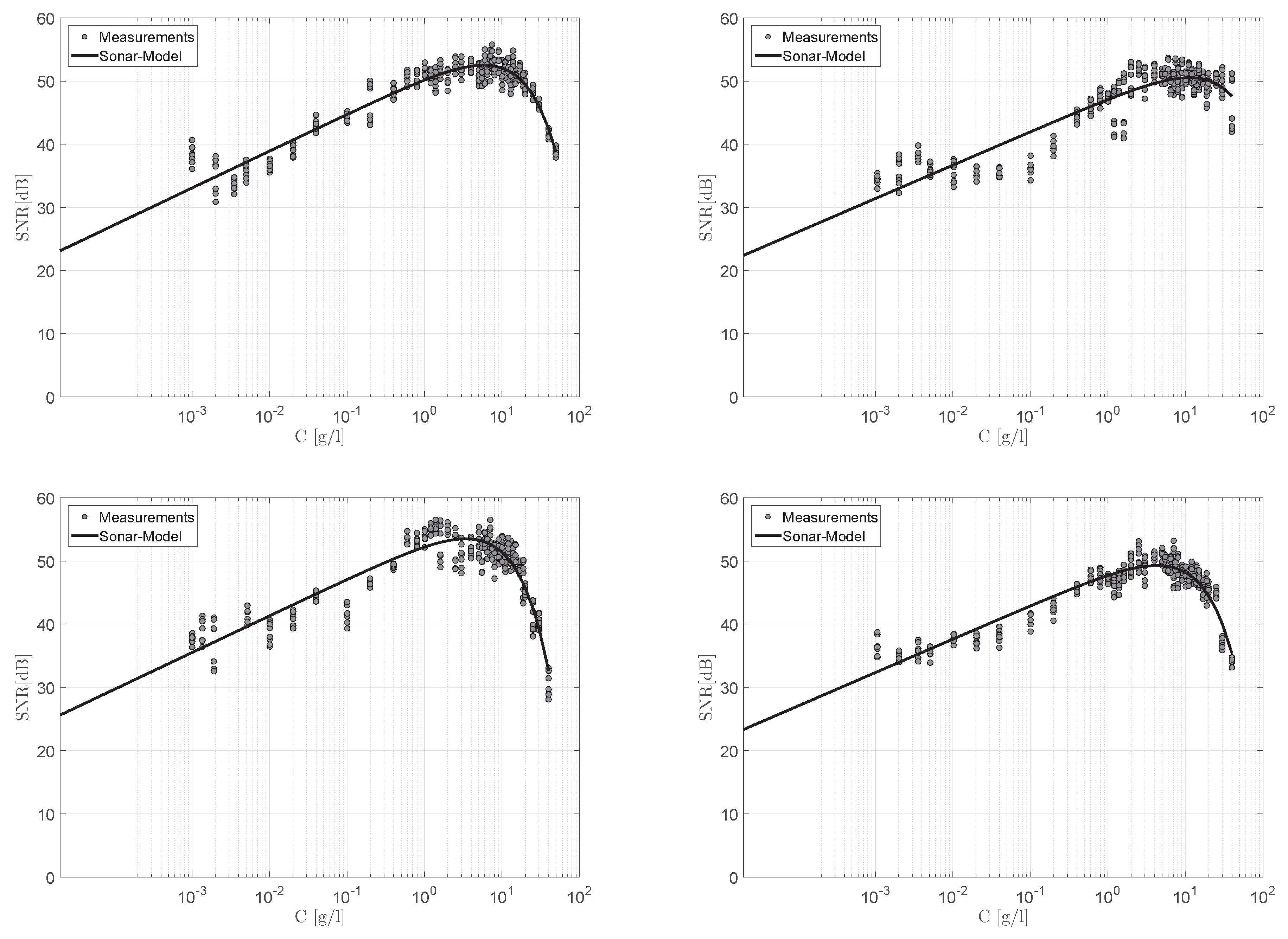
After repeating the calibration experiment for different sediments, the sonar model was fitted to the measurements. The results for the artificial sediments (quartz powder, bentonite, metakaolin, and Chinafill) are plotted in Figure 7. It can be seen that the sonar model was capable of reproducing the experimental datasets.

In the case of artificial sediments, it is recognizable that there was some deviation between the model and the experimental data in the log-linear regime (II: audibility zone). However, with increasing concentration, the deviations become smaller. When the concentration was sufficiently high, a decrease of the SNR was observed. The conditions to pass from increasing to decreasing SNR response (III: muffling zone) differed with the type of sediment.

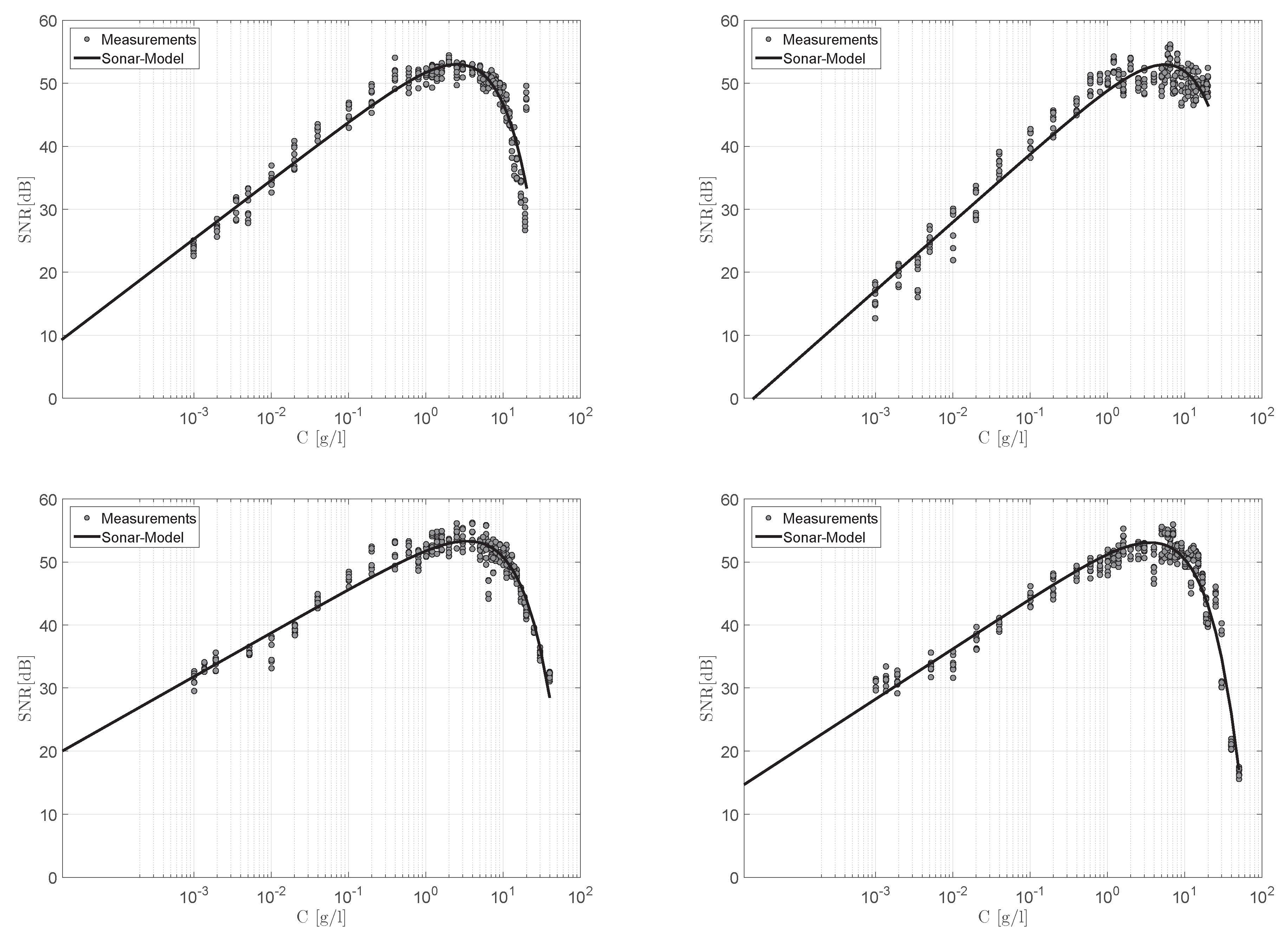
In comparison to the artificial sediments, the natural sediments from Lake Eixendorf, Lake Altmühl, and the Ems Estuary are presented in Figure 8. The resulting fit parameters are summarized in

Table 3. Fit parameter of the sonar model for different sediments. $R^2$ as a statistical parameter is the square of the correlation between the fitted and the measured values.

Material/Location	${\mathsf{\Pi }}_1$ (-)	${\mathsf{\Pi }}_2$ (-)	${\mathit{C}}_{\mathit{ADV}}$ (dB)	${\mathit{R}}^2$ (%)
Quartz powder	1.712	4.34	42.08	96.34
Bentonite	1.890	0.94	57.06	88.91
Metakaolin	1.719	4.57	54.98	91.02
Chinafill	1.887	3.08	55.54	92.99
Ems 2012	1.441	4.47	38.84	96.32
Ems 2015	1.253	7.40	20.62	95.69
Lake Eixendorf	1.070	11.06	10.97	88.34
Lake Altmühl	0.921	3.37	6.27	96.59

for all measurements. Additionally, $R^2$ is given as the square of the correlation between the fitted and the measured values.

Even for natural sediments where the composition of sediment is far more complex compared to artificial sediments, our sonar model was able to reproduce the experimental data. Furthermore, it seems that natural sediments rather follow a log-linear approach in the low concentration regime (II: audibility zone) than artificial sediments. For natural sediments, the slope of the modeling results in the log-linear regime does not differ as much as for the artificial sediments. In the opinion of the authors, this effect is not surprising since natural sediments likely consist of similar sediment partitions.

For natural sediments, the vertices of the modeled SNR were located very close to each other, whereas the variation was greater for artificial sediments. Out of this, we conclude that there exists a sediment- and device-specific critical concentration, which separates the increasing and decreasing SNR response.

5. Discussion

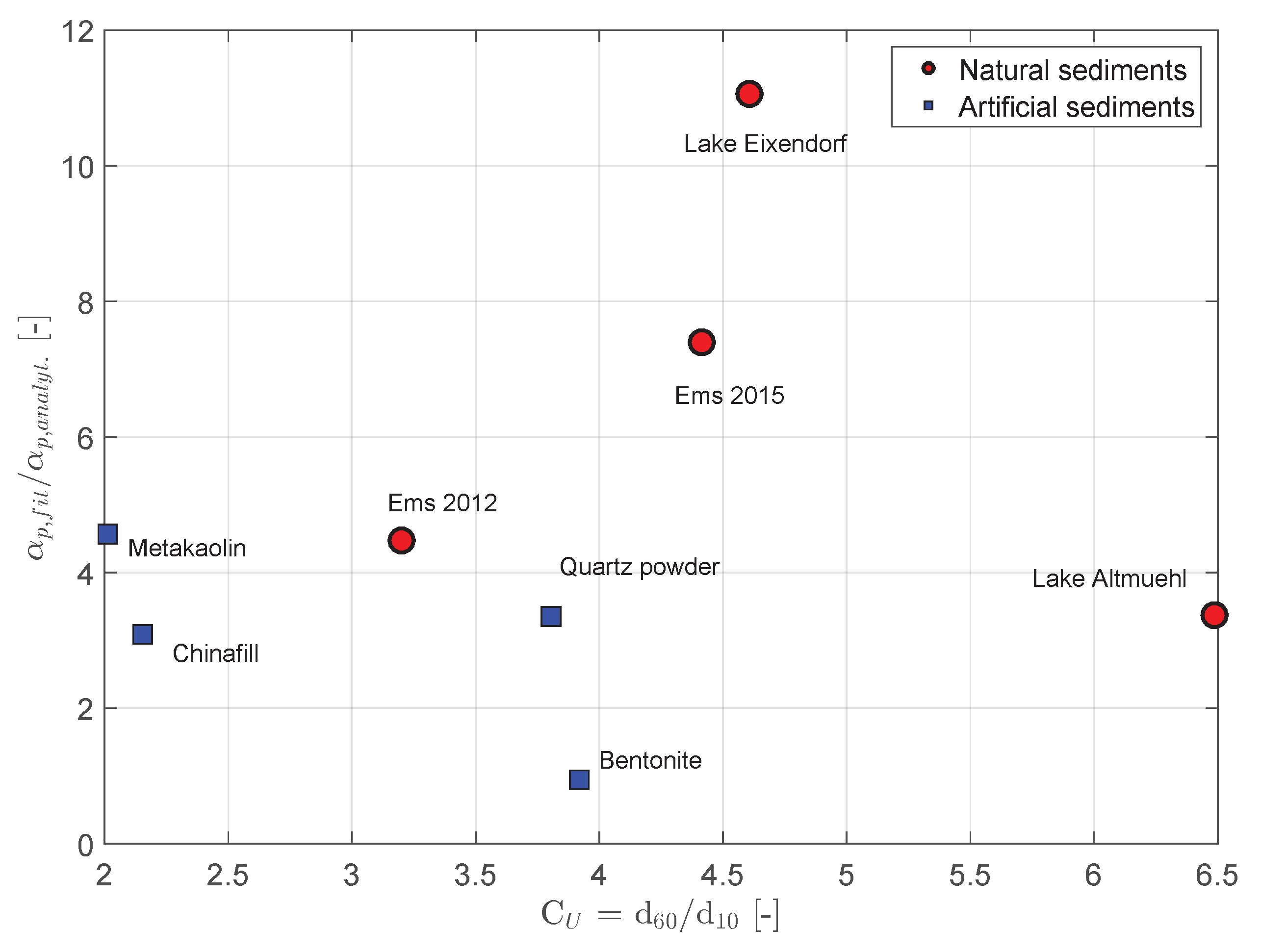
We analyzed the fit parameters ${\Pi }_2$ and $C_{ADV}$ and separated the data into artificial sediments (quartz powder, bentonite, metakaolin, and Chinafill) and natural sediments (Ems Estuary, Lake Eixendorf, and Lake Altmühl). Knowing that the mentioned artificial sediments are natural materials, but artificially processed, we use this terminus to distinguish between the sediments extracted from nature. When reading the fit parameters in Table 3, differences between ${\Pi }_2$ and $C_{ADV}$ can be observed. Furthermore, it can be seen that ${\Pi }_2$ and $C_{ADV}$ can be separated into artificial and natural sediments. This is shown in Figure 9 for ${\Pi }_2$ and in Figure 10 for $C_{ADV}$. ${\Pi }_2$ is described through ${\alpha }_{p,fit}$/${\alpha }_{p,analyt.}$, which is the coefficient of the fitted and the analytically-calculated particle absorption coefficient. A value close to one would imply perfect agreement between the modeled sound absorption on particles and the value based on Urick’s formula in Equation (12).

Artificially-processed sediments are characterized by a very homogeneous grain size distribution, which is not or to a negligible extent contaminated by other sediments or particle diameters. The grading curve therefore is steeper than for sediments extracted from nature. The uniformity coefficient $C_U$ = $d_{60}$/$d_{10}$ is a dimensionless number to describe the uniformity of a sediment sample. The diameters $d_{60}$ and $d_{10}$ correspond to 60% and 10% sieve passage, respectively. The sediment samples’ uniformity coefficients $C_U$ are shown in Table 2. The grading curves of the artificial sediments result in lower $C_U$-values than for natural sediments. The formula of Urick (Equation (12)), which is implemented in the model, is based on the assumption of homogeneous particle diameters [7]. In Salehi and Strom, it is mentioned that the particle size distribution also affects ${\alpha }_p$ [5]. In the case of ideal sediment, where all particles have the same size, $C_U$ would be equal to one. This was not the case, no matter which sediment we used. However, in Figure 9, it is shown that ${\alpha }_{p,fit}$/${\alpha }_{p,analyt.}$ is lower when using artificial sediments with lower $C_U$ values. However, as the data for “Ems 2012” show, $C_U$ is not the only parameter that leads to a decrease of ${\alpha }_{p,fit}$/${\alpha }_{p,analyt.}$. “Ems 2012” with $C_U$ = 3.2 results in ${\alpha }_{p,fit}$/${\alpha }_{p,analyt.}$ = 4.47, which is greater than the values of quartz powder and bentonite.

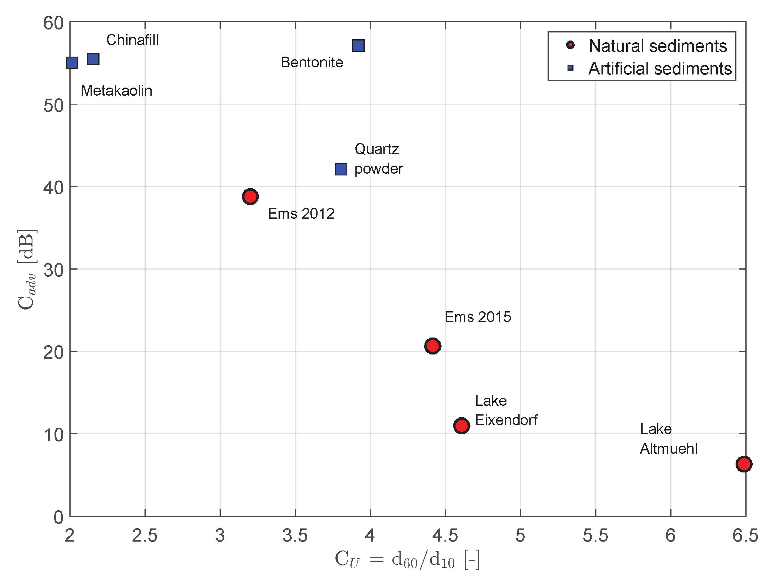
Figure 10 presents the fit parameter $C_{ADV}$ with respect to $C_U$. Our results show that $C_{ADV}$ is not only a device-specific parameter, which can be kept as constant for every material. We conclude that it is rather a combined device- and sediment-specific parameter. The data for $C_{ADV}$ again can be separated into artificial and natural sediments and were in the range of $C_{ADV}$ = 42–58 dB for quartz powder, bentonite, Chinafill, and metakaolin. On the contrary, $C_{ADV}$ data for natural sediments were in the range of $C_{ADV}$ = 6–39 dB.

To summarize, our results show that the sonar model can be applied for different sediments without losing its qualitative behavior. We also showed that the model parameters clearly indicate the variation of sediment type. It was shown that the sediment absorption coefficients ${\alpha }_p$ and $C_{ADV}$ not only rely on the sediment diameter, but also on the grain size distribution.

Practical Use and Reliability

In order to assess the practical use, applicability, and reliability of measurements in rivers and estuaries, for instance, we highlight some main characteristics of the method.

Due to the model’s dependence on the particle grain size distribution, the user in the field would need to specify the characteristic sediment that occurs at the measurement location. When Urick’s sound absorption coefficient is used, the mean particle radius and the solid density are needed.

Next, with respect to the sediment-specific parameters, knowledge about the measurement device (here: ADV) is necessary. In general, the sonar model can be also applied for ADCP measurements (e.g., [11,27]), though within this study, we only discuss ADV measurements. The ADV probe (Nortek, Vectrino Profiler) that was used has a dynamic range of 60 dB. In comparison, the Vectrino+ (Nortek) has a dynamic range of 25 dB. Both probes have an emitter frequency of 10 MHz. When repeating our measurements with the Vectrino+ probe, we could not find any trend between the SNR and the concentration. Therefore, it can be concluded that a certain dynamic range is of importance to resolve the SNR response with respect to the concentration. Furthermore, it is mentioned that the presented parameters are only valid for the Vectrino Profiler with a dynamic range of 60 dB.

Following the SNR function to concentrations lower than 0.1 mg/L, one will perceive that in this case, Equation (14) predicts negative SNR values. In particular for C = 3 × 10${}^{-6}$ g/L, the function crosses the axis of ordinate at SNR = −10 dB. Following the principles of the sonar theory, the SNR has to be positive for particle detection [25]. Negative values of the SNR would imply that noise is more dominant compared to the particle backscatter signal. Thus, the region of negative SNR values should be neglected for the interpretation of the model function based on sonar theory. Additionally, it can be observed that the experimental SNR data seem to reach a minimum threshold value for concentrations close to zero. This is explained by the SNR definition, which is implemented in the software of the measuring device. Within the ADV probe, the SNR is calculated by the difference of the backscatter signal intensity, which is here called Amp${}_b$ (dB), and the noise intensity, Amp${}_n$ (dB):

$$SNR=Am{p}_b-Am{p}_n$$

(15)

Each of the two intensities is calculated by the received counts as:

$$Am{p}_i=20lo{g}_{10}\left(\frac{count{s}_i+1}{count{s}_{max}}\right)$$

(16)

with counts${}_{max}$ = 8000 for the used ADV probe [28]. This formulation leads to a minimum intensity Amp${}_{min}$ = −78.062 dB for no detected counts and to a maximum intensity Amp${}_{max}$ = 0 dB in the case of reaching the maximum counts. When inserting Equation (16) into Equation (15), the SNR is written as:

$$\begin{array}{c}\hfill SNR=20lo{g}_{10}\left(\frac{count{s}_b+1}{count{s}_n+1}\right)=20lo{g}_{10}\left(\frac{count{s}_p+count{s}_n+1}{count{s}_n+1}\right)\end{array}$$

(17)

where counts${}_b$ includes the counts related to particle backscattering counts${}_p$, as well as the noise counts${}_n$. In the case of no backscatter intensity (absolutely no scattering particles in the measurement volume), the minimum SNR would be SNR${}_{min}$= 0 dB and fully independent of noise intensity. Indeed, this is a theoretical threshold, because there are always some scattering particles in the measurement volume. Nevertheless, there is a minimum threshold value for the SNR, which cannot be reproduced by the log-linear sonar model.

Assuming well-mixed conditions in the experimental tank, depth and bottom material are not expected to influence the SNR. As the name signal-to-noise ratio says, it describes the sound intensity of the ratio of the received signal and the background noise. In practice, just before measuring, the ADV probe records the noise intensity. Later during the active measurements, this intensity is subtracted from the absolute received signal (amplitude). Of course, depth and bottom material can influence the intensity of noise. However, the SNR is not influenced by this. This makes the SNR a reliable and universal measure for different environments. However, it has to be noted that the device’s technique to determine the SNR is only valid for steady noise intensity. When conducting long-term measurements with frequent changes of noise (ships, wind, etc.) during the data acquisition, the SNR will be falsified.

In our experiments, we tried to avoid flocculation of particles while the suspension was well mixed. In nature, especially in estuaries, various floc populations are observed, e.g., [29]. Sound attenuation on flocs is expected to be different than on single primary particles. Flocs are a connection of solids and organic substances, which vary in size, density, and elasticity. In order to calibrate the probe for flocculated suspensions, advanced experimental setups are needed where flocs will not be destroyed during the experiment.

Summing up, the sonar model is able to reproduce the experimental data for a number of different sediments. It shows the log-linear increase of SNR with concentration, as well as the vertex behavior and the decrease of SNR for higher concentrations. This particular behavior of the SNR (increase and decrease) expects attention and special treatment when applying such a model for concentration measurements in nature. One SNR value can be assigned to two concentrations, which is a disadvantage of the model and which has to be taken into account. It reduces the measurement range of this method either to the low concentration regime (positive slope of SNR) or to the high concentration regime (negative slope of SNR). While only using the ADV probe for concentration measurements, the user will not be able to assess the appropriate concentration. Especially in nature, the usage of a second concentration measurement device (e.g., OBS, LISST, tuning fork, etc.) would be necessary to specify the concentration regime [6,11,30]. Then, it is possible to utilize an ADV to measure the velocity, the turbulence, and the concentration simultaneously.

6. Conclusions

In the scope of the experimental investigations, a clear relation was found between the SNR and the concentration of several sediment suspensions. The method was found to be valid for maximum concentrations $C_{max}$ = 50 g/L, as is shown for sediments from the Ems Estuary. In higher concentrations, correlation values between two received signals dropped below 70 %, that is why those measurement results were discarded within the evaluation [31]. While combining scattering and sonar theory, an advanced model was presented for computing the concentration out of the SNR for natural and artificial sediments. The derived model parameters are only valid for the ADV probe and the sediments that we used in this experiment. However, it was shown that the methodology is valid for different sediments, both natural or artificial ones, and it can be applied for further investigations of turbulent suspension flows. Since this measurement technique allows temporal high resolved (f = 100 Hz) non-invasive concentration measurements, it is meant to be a basis for further experimental investigations of turbulence and diffusivity, either in nature or at the laboratory scale.

References

1. Nezu, I.; Nakagawa, H. Turbulence in Open-Channel Flows. J. Fluid Mech. 1994, 269, 373–374. [Google Scholar] [CrossRef]
2. Schrottke, K. Dynamik fluider Schlicke im Weser und Ems-Ästuar—Untersuchung und Analysen zum Prozessverständnis; BAW/BfG Kolloqium: Karlsruhe, Germany, 2006. [Google Scholar]
3. Cellino, M. Experimental Study of Suspension Flow in Open Channels. Ph.D. Thesis, Ecole Polytechnique Federale de Lausanne, Lausanne, Switzerland, 1998. [Google Scholar]
4. Pope, S.B. Turbulent Flows; Cambridge University Press: Cambridge, UK, 2001. [Google Scholar]
5. Salehi, M.; Strom, K. Using Velocimeter Signal to Noise Ratio as a Surrogate Measure of Suspended Mud Concentration. Cont. Shelf Res. 2011, 31, 1020–1032. [Google Scholar] [CrossRef]
6. Fugate, D.C.; Friedrichs, C.T. Determining concentration and fall velocity of estuarine particle populations using ADV, OBS and LISST. Cont. Shelf Res. 2002, 22, 1867–1886. [Google Scholar] [CrossRef]
7. Urick, R. The absorption of sound in suspensions of irregular particles. J. Acoust. Soc. Am. 1948, 20, 283–289. [Google Scholar] [CrossRef]
8. Lohrmann, A.; Cabrera, R.; Kraus, N.C. Acoustic-Doppler Velocimeter (ADV) for Laboratory Use. In Proceedings of the Fundamental and Advancements in Hydraulic Measurements and Experimentation, Buffalo, NY, USA, 1–5 August 1994; pp. 351–365. [Google Scholar]
9. Thorne, P.D.; Hanes, D.M. A review of acoustic measurement of small-scale sediment processes. Cont. Shelf Res. 2002, 22, 603–632. [Google Scholar] [CrossRef] [Green Version]
10. Jay, D.A.; Orton, P.; Kay, D.J.; Fain, A.; Baptista, A.M. Acoustic determination of sediment concentrations, settling velocities, horizontal transports and vertical fluxes in estuaries. In Proceedings of the IEEE Sixth Working Conference on Current Measurement, San Diego, CA, USA, 13 March 1999; pp. 258–263. [Google Scholar]
11. Hoitink, A.; Hoekstra, P. Observations of Suspended Sediment from ADCP and OBS Measurements in a Mud-dominated Environment. Coast. Eng. 2005, 52, 103–118. [Google Scholar] [CrossRef]
12. Ha, H.; Hsu, W.Y.; Maa, J.Y.; Shao, Y.; Holland, C. Using ADV backscatter strength for measuring suspended cohesive sediment concentration. Cont. Shelf Res. 2009, 29, 1310–1316. [Google Scholar] [CrossRef]
13. Decrop, B.; De Mulder, T.; Toorman, E.; Sas, M. New methods for ADV measurements of turbulent sediment fluxes–application to a fine sediment plume. J. Hydraul. Res. 2015, 53, 317–331. [Google Scholar] [CrossRef]
14. Best, J.; Bennet, S.; Bridge, J.; Leeder, M. Turbulence Modulation and Particle Velocities over Flat Sand Beds at Low Transport Rates. J. Hydraul. Eng. 1997, 123, 1118–1129. [Google Scholar] [CrossRef]
15. Cellino, M. Ultrasonic Measurements of Instantaneous Velocity and Suspended Concentration in Open-Channel Flow. In Proceedings of the Third International Symposium on Ultrasonic Doppler Methods for Fluid Mechanics and Fluid Engineering Co-organized by EPFL and PSI, Lausanne, Switzerland, 9–11 September 2002. [Google Scholar]
16. Hurther, D.; Thorne, P.D.; Bricault, M.; Lemmin, U.; Barnoud, J.M. A multi-frequency Acoustic Concentration and Velocity Profiler (ACVP) for boundary layer measurements of fine-scale flow and sediment transport processes. Coast. Eng. 2011, 58, 594–605. [Google Scholar] [CrossRef]
17. Revil-Baudard, T.; Chauchat, J.; Hurther, D.; Barraud, P.A. Investigation of sheet-flow processes based on novel acoustic high-resolution velocity and concentration measurements. J. Fluid Mech. 2015, 767, 1–30. [Google Scholar] [CrossRef] [Green Version]
18. McAnally, W.H.; Friedrichs, C.; Hamilton, D.; Hayter, E.; Shrestha, P.; Rodriguez, H.; Sheremet, A.; Teeter, A. Management of Fluid Mud in Estuaries, Bays, and Lakes. I: Present State of Understanding on Character and Behavior. J. Hydraul. Eng. 2007, 133, 9–22. [Google Scholar] [CrossRef]
19. Becker, M.; Maushake, C.; Winter, C. Observations of Mud-Induced Periodic Stratification in a Hyperturbid Estuary. Geophys. Res. Lett. 2018, 45, 5461–5469. [Google Scholar] [CrossRef]
20. Craig, R.G.; Loadman, C.; Clement, B.; Rusello, P.J.; Siegel, E. Characterization and testing of a new bistatic profiling acoustic Doppler velocimeter: The vectrino-II. In Proceedings of the 2011 IEEE/OES 10th Current, Waves and Turbulence Measurements (CWTM), Monterey, CA, USA, 20–23 March 2011; pp. 246–252. [Google Scholar]
21. Thomas, R.; Schindfessel, L.; McLelland, S.; Creëlle, S.; De Mulder, T. Bias in mean velocities and noise in variances and covariances measured using a multistatic acoustic profiler: The Nortek Vectrino Profiler. Meas. Sci. Technol. 2017, 28, 075302. [Google Scholar] [CrossRef]
22. Bruens, A. Communications on Hydraulic and Geotechnical Engineering—Entraining Mud Suspensions; Report No. 03-1; Delft University of Technology: Delft, The Netherlands, 2003. [Google Scholar]
23. Mietta, F.; Chassagne, C.; Winterwerp, J. Shear-induced flocculation of a suspension of kaolinite as function of pH and salt concentration. J. Colloid Interface Sci. 2009, 336, 134–141. [Google Scholar] [CrossRef] [PubMed]
24. Medwin, H.; Clay, C.S. Fundamentals of Acoustical Oceanography; Academic Press: Cambridge, MA, USA, 1997. [Google Scholar]
25. Lerch, R.; Sessler, G.; Wolf, D. Technische Akustik: Grundlagen und Anwendungen; Springer: Berlin/Heidelberg, Germany, 2009. [Google Scholar]
26. Lohrmann, A. Monitoring Sediment Concentration with Acoustic Backscattering Instruments; Nortek Technical Note; Nortek: Bologna, Italy, 2001; p. 9. [Google Scholar]
27. Guerrero, M.; Szupiany, R.N.; Latosinski, F. Multi-frequency acoustics for suspended sediment studies: An application in the Parana River. J. Hydraul. Res. 2013, 51, 696–707. [Google Scholar] [CrossRef]
28. AS Nortek. VECTRINO Velocimeter User Guide (Rev. C); AS Nortek: Carlsbad, CA, USA, 2004. [Google Scholar]
29. Dyer, K.; Manning, A. Observation of the size, settling velocity and effective density of flocs, and their fractal dimensions. J. Sea Res. 1999, 41, 87–95. [Google Scholar] [CrossRef]
30. Groposo, V.; Mosquera, R.L.; Pedocchi, F.; Vinzón, S.B.; Gallo, M. Mud Density Prospection Using a Tuning Fork. J. Waterw. Port Coast. Ocean Eng. 2015, 141, 04014047. [Google Scholar] [CrossRef]
31. Ali, A.; Lemckert, C.J. A traversing system to measure bottom boundary layer hydraulic properties. Estuar. Coast. Shelf Sci. 2009, 83, 425–433. [Google Scholar] [CrossRef] [Green Version]
Figure 1. Sound intensities, which are of importance to state the sonar balance equation.
Acoustics 01 00006 g001
Figure 2. The experimental setup is shown for calibrating the ADV’s SNR and the concentration. The sketch is showing the stirrer and the ADV probe in side view, and the photograph is showing the experiment in top view.
Acoustics 01 00006 g002
Figure 3. A box plot evaluation is shown of the SNR data for three repeated measurements in a low concentrated quartz powder suspension. Only negligible deviations of the median of each beam are recognizable.
Acoustics 01 00006 g003
Figure 4. The evaluation of the frequency of measured SNR data is described in histograms (Run 03). Histograms are given for each receiver (beam) with corresponding mean and standard deviation values.
Acoustics 01 00006 g004
Figure 5. SNR measurements are shown for two different measurement heights as a function of the quartz powder concentration. Measurement results of each receiver are summarized. For better interpretation, the curve is divided into three characteristic areas (I, II, III).
Acoustics 01 00006 g005
Figure 6. The measured SNR data are shown as a function of quartz powder concentration. The fit function is given for the evaluation of the sonar equation (Equation (14)). This model predicts a decreasing SNR in the high concentration regime and a log-linear development in the low concentration regime.
Acoustics 01 00006 g006
Figure 7. The measured SNR data are shown as a function of concentration for different artificial sediments: (upper left) quartz powder; (upper right) bentonite; (lower left) metakaolin; (lower right) Chinafill. The fit function is given for the evaluation of the sonar equation (Equation (14)). This model predicts a decreasing SNR in the high concentration regime and a log-linear development in the low concentration regime.
Acoustics 01 00006 g007
Figure 8. The measured SNR data are shown as a function of concentration for different artificial sediments: upper left: Lake Eixendorf: upper right: Lake Altmühl; lower left: Ems 2012; lower right: Ems 2015. The fit function is given for the evaluation of the sonar equation (Equation (14)). This model predicts a log-linear evolution in the low concentration regime and a decreasing SNR in the high concentration regime.
Acoustics 01 00006 g008
Figure 9. Artificial sediments have lower uniformity coefficients C U than natural sediments. This results in lower values of α p , f i t / α p , a n a l y t . , which means that the agreement increases towards the formula of Urick.
Acoustics 01 00006 g009
Figure 10. Artificial sediments have lower uniformity coefficients C U than natural sediments. As a result, the sonar model predicts greater C A D V values.
Acoustics 01 00006 g010