Quantitative Morphological Analysis of Rust Streak Formation and Underlying Substrate Profile Changes Under Controlled Droplet Supply

Abstract

This study quantitatively analyzed rust-streak formation under controlled droplet supply and its relationship with the rust-removed surface profile of the substrate. A NaCl aqueous solution was dropped at a constant flow rate onto SPCC steel plates inclined at 70° to observe the temporal development of the rust streak. Surface line profiles before and after the removal of red rust were measured, and profile changes were quantified relative to the initial surface. Rust layer height $h_{\mathrm{rust}}\left(x\right)$ and rust-removed surface profile $z_{\mathrm{r}}^{\ast }\left(x\right)$ were determined, and their distributions and integrated values were compared. The rust width reached approximately 2.5–3.0 mm, comparable to the droplet diameter under the present conditions. Downstream, rust layer height increased with the extension of test duration, whereas the integrated profile of the rust-removed surface remained relatively small. Rust layer height and rust-removed surface profile were not directly related at each observation position L. These results suggest that rust streak formation within the tested parameter window involves not only locally formed rust but also rust carried from upstream by liquid flow, and indicate that visible rust morphology alone cannot adequately represent substrate-side profile changes under these specific conditions.

1. Introduction

Under atmospheric corrosion conditions, corrosion products and dissolved metal species can be removed from the metal surface by liquids such as rainwater (metal runoff), followed by redistribution and deposition in downstream regions [1,2,3]. Herein, streak-like corrosion features formed through this process are defined as rust streaks. In natural environments, rainwater is often considered a representative liquid responsible for rust transport [4], whereas seawater also contributes to this process in coastal regions. This phenomenon is not merely an aesthetic change but involves at least three steps: (i) rust formation owing to substrate corrosion, (ii) transport and runoff of rust by liquid, and (iii) attachment and lateral growth in downstream regions. These steps are not strictly independent and may proceed simultaneously under actual exposure conditions. Consequently, visible rust streaks reflect the combined effects of locally formed rust and rust transported by liquid flow. However, the contribution of transport to this process has rarely been systematically quantified.

The electrochemical mechanisms of substrate corrosion (step i) have been extensively studied [5,6,7,8]. Rust transport and metal-ion runoff (step ii) have been investigated mainly from an environmental perspective [7,9,10,11]. Rust attachment and expansion (step iii) have been examined primarily in the context of the staining of cultural heritage materials and architectural facades [4,12,13,14,15]. In actual structures, moisture retention frequently occurs in uneven regions and gaps, particularly at welded joints. Corrosion originating from weld-specific microstructures and defects [16,17,18,19] can be accelerated under such conditions [20]. Even the simple ingress and retention of moisture in crevices is sufficient for promoting corrosion [21], with such localized corrosion sites suggested as initiation points for rust streak formation.

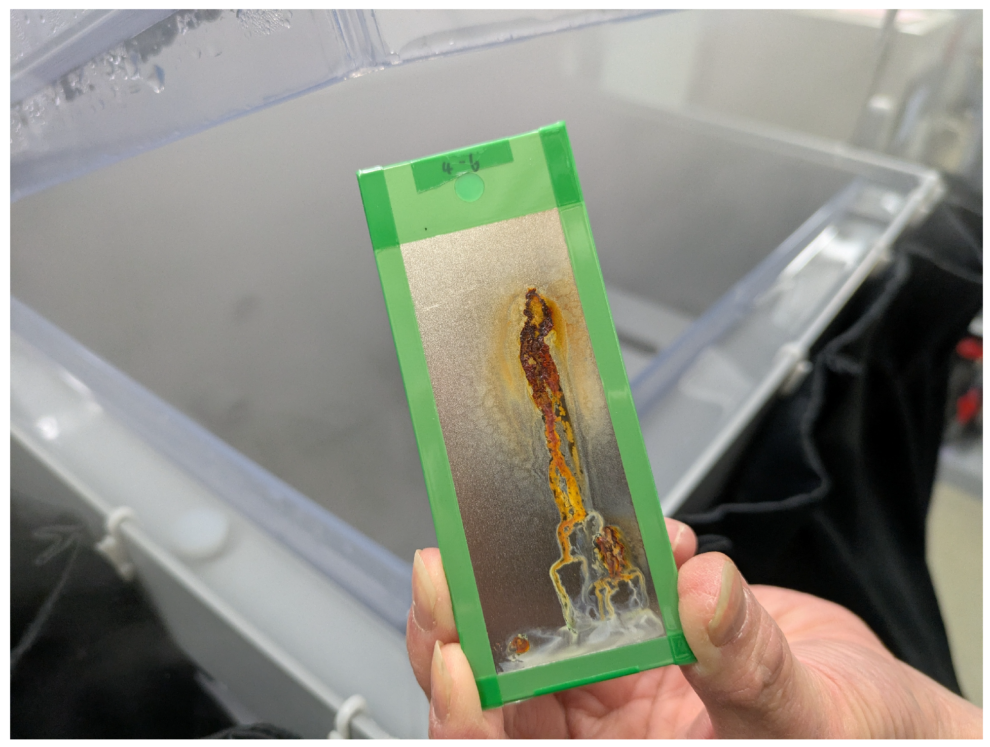
Several studies have investigated the relationship between corrosion phenomena and outdoor environmental factors, such as rainfall, installation orientation, inclination angle [22,23], and pH conditions [1]. As a controlled alternative to regionally variable outdoor exposure, the salt spray test is widely used for evaluating corrosion resistance [24,25]. In this test, an atomized salt solution flows down an inclined surface, resulting in rust streak formation (Figure 1). The salt spray test provides a reproducible platform for the simultaneous observation of liquid flow, rust formation, and deposition under controlled conditions.

In salt spray testing, appearance change is widely used as an evaluation criterion. Monitoring-equipped systems have been developed to enhance inspection stability and efficiency, and these systems have begun to reveal the influence of rust expansion behavior and rust streak formation on visible appearance [26,27]. However, the spatial distribution of substrate corrosion beneath rust streaks remains insufficiently evaluated. Although numerous studies have focused on corrosion mass loss and metal runoff, quantitative analyses of the morphological development of rust streaks remain limited. Studies on metal runoff have mainly focused on concentration and ionic species [1].

Quantitative investigations of rust transport by liquid flow and the associated spatial distribution of changes in surface morphology and stain propagation are still scarce. In particular, systematic comparisons of (i) rust streak morphology, (ii) local changes in the substrate profile beneath them, and (iii) their spatial correlations under controlled liquid supply conditions on the same specimen are limited.

Therefore, it remains unclear whether rust streaks are merely deposited layers or whether corrosion progresses directly beneath them. Based on this background, the present study establishes an experimental system with controlled liquid supply conditions to quantitatively evaluate the morphological development of rust streaks and the changes in the profile of the underlying substrate on the same specimen. The objectives are (i) to quantify the morphological development of rust streaks under controlled droplet supply, (ii) to spatially evaluate changes in the substrate profile beneath rust streaks, and (iii) to clarify the relationship between the two.

2. Materials and Methods

2.1. Materials and Corrosive Solution

As shown in

Table 1. Material and solution parameters.

Materials
Base material	Cold-rolled low-carbon steel sheet
Base material composition (wt.%)	C 0.05, Mn 0.19, P 0.020, S 0.013
Test specimen dimensions (mm)	150 × 70 × 0.8
Surface roughness (µm)	Ra 2.1, Rp 5.1
Static contact angle (°)	77.6
Corrosion acceleration solution
Solute	Sodium chloride only
Concentration (g/L)	50 ± 5
pH	6.5–7.2

, cold-rolled low-carbon steel sheets (SPCC-SD, conforming to the Japanese Industrial Standard JIS G 3141) with a dull finish were used as the substrate material in the present study. The representative chemical composition listed in the mill sheet was C 0.05 wt.%, Mn 0.19 wt.%, P 0.020 wt.%, and S 0.013 wt.%, with all elemental contents within the upper limit specified for EN DC01. The specimen dimensions were 150 mm × 70 mm × 0.8 mm. The specimens were used in the as-received condition, without any additional surface treatment applied. Before testing, the specimens were degreased with ethanol (Hayashi Pure Chemical Ind., Ltd., Osaka, Japan) and dried in air for at least one hour.

Surface roughness and static contact angle were measured as initial substrate characteristics. Surface roughness was measured using laser scanning microscopy (VR-3000/VR-3200, KEYENCE Corporation, Osaka, Japan), and the static contact angle was measured using a contact angle meter (DMo-602, Kyowa Interface Science Co., Ltd., Niiza, Japan). Surface roughness and static contact angle were measured using nine specimens, with three measurement points per specimen (27 points in total). Within the evaluation length of 4 mm, R_a had a median value of 2.1 µm with an interquartile range of 1.6–2.3 µm. The maximum peak height above the mean line (R_p) showed a median of 5.1 µm with an interquartile range of 4.4–5.7 µm. The static contact angle had a median value of 77.6° with an interquartile range of 77.0–78.6°, which is consistent with the generally accepted range for metallic surfaces [28].

The corrosive solution was prepared by dissolving analytical-grade sodium chloride (Hayashi Pure Chemical Ind., Ltd., Osaka, Japan) in pure water to a concentration of 50 ± 5 g/L. The NaCl solution was prepared with reference to the solution parameters (concentration and pH range) specified in ISO 9227 [25] for the salt spray test. Herein, a liquid supply system was designed to investigate rust-streak formation under conditions relevant to salt spray testing, particularly those associated with droplet runoff, retained-liquid movement, and rust transport/redeposition. Therefore, although the actual spray environment was not reproduced, the present design intentionally adopted a parameter window relevant to these salt-spray-related phenomena.

2.2. Experimental Setup and Test Conditions

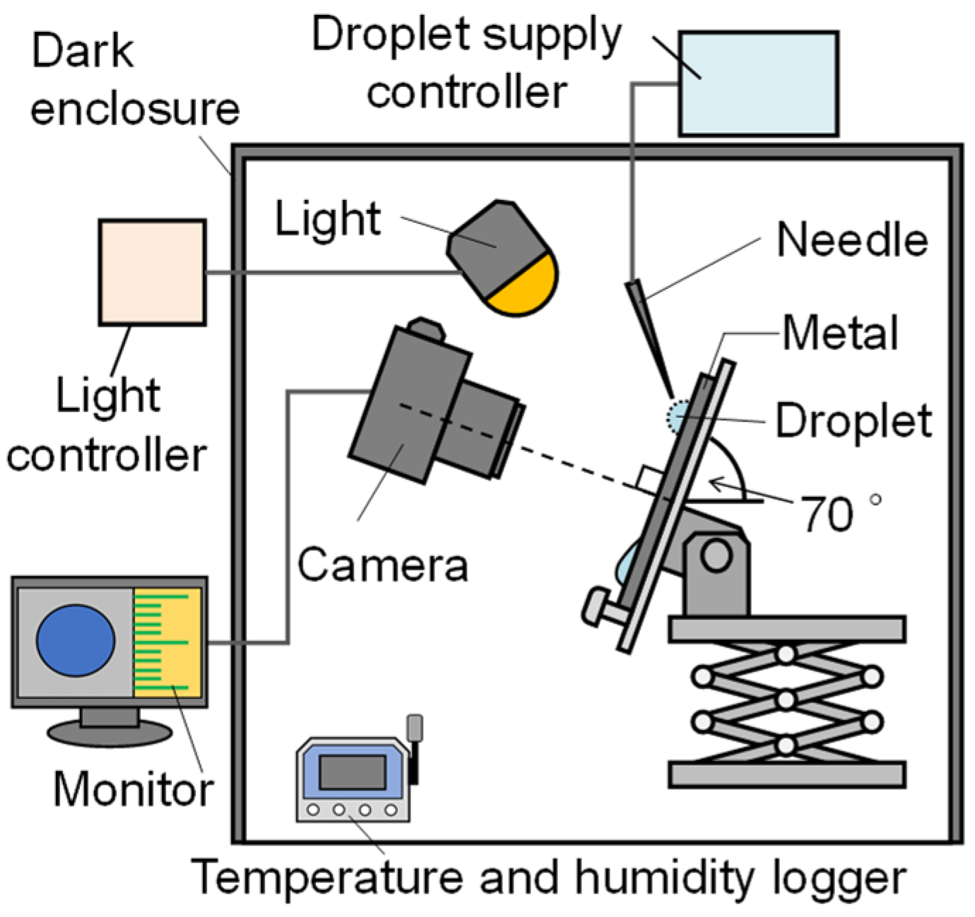
The experimental setup and experimental conditions are presented in Figure 2 and

Table 2. Experimental parameters.

Experimental Conditions
Saltwater supply rate (µL/min)	10, 30, and 60
Test duration (min)	300, 600, and 1900 *
Specimen tilt angle (°)	70
Imaging intervals (min)	10
Test temperature (°C)	15–20
Test humidity (%)	40–50

* Only for a supply rate of 10 µL/min.

. The NaCl solution was supplied from a needle tip (inner diameter of 0.41 mm, outer diameter of 0.71 mm, 22G; NN-2238N, Terumo Corporation, Tokyo, Japan), with supply flow rate Q and duration t controlled using a syringe pump (YSP-101, YMC Co., Ltd., Kyoto, Japan). The solution was supplied as intermittent droplets rather than a continuous flow. For example, under a supply rate of Q = 30 µL/min, 20 ± 1 droplets were delivered within 10 min. The volume per droplet was approximately 14.1 µL (mass of approximately 14.4 mg), and the droplet diameter was approximately 3 mm. This diameter was calculated by measuring the mass of a single droplet and converting it to volume, assuming a density of 1.0 g/cm³ and a spherical shape.

Although the needle position was fixed, slight variations in the droplet landing position may occur depending on droplet formation conditions. However, the droplet impact area was confined within a region considerably smaller than the characteristic width of the rust streaks analyzed herein. The supply rate (Q) was set to 10, 30, and 60 µL/min, and the supply duration (t) was 300 or 600 min. In addition, a long-duration experiment was conducted at Q = 10 µL/min for 1900 min. The specimen was fixed at an inclination angle of 70° relative to the horizontal plane (20° relative to the vertical plane). This angle falls within the inclination range (15–30° relative to the vertical plane) specified in ISO 9227 [25] and was adopted here as a salt-spray-test-relevant inclination rather than as a variable for evaluating angle dependence. Together with the selected NaCl condition and the monitored environmental range, this inclination was adopted to capture salt-spray-relevant liquid-flow phenomena such as droplet runoff, retained-liquid movement, and rust transport/redeposition, rather than to cover a broad environmental matrix.

Under each condition, photographs were taken every 10 min from the start of droplet supply using a digital camera (Pentax K10D, RICOH IMAGING COMPANY, Ltd., Tokyo, Japan) with an 18–55 mm lens. The shooting conditions were f/8, 0.8 s, and ISO 400. To suppress specimen heating, lighting was turned on only during photography, and experiments were conducted inside a dark enclosure. The experiments were conducted at 15–20 °C (room temperature) and 40–50% relative humidity inside the enclosure, as monitored using a humidity logger (LR5001, HIOKI E.E. CORPORATION, Ueda, Japan). These values were treated as monitored ambient ranges during the experiment rather than as tightly controlled independent variables. The number of trials for each condition was n = 1. The present study focused on the systematic characterization of spatial correlations within individual specimens under a salt-spray-relevant liquid-flow condition rather than on statistical variability between specimens or the strict evaluation of temperature, humidity, or angle dependence. The present results should therefore be interpreted as case-specific morphological observations within the tested parameter window rather than as statistically generalizable trends across specimens. The reproducibility and scatter of these trends across specimens remain subjects for future study using repeated experiments.

2.3. Removal of Corrosion Products

After each experiment, red rust was removed from the substrate surface using an aqueous solution of diammonium hydrogen citrate (FUJIFILM Wako Pure Chemical Corporation, Osaka, Japan). This solution has been used for removing rust from iron-based materials in previous studies, particularly in precleaning before experiments [29], corrosion weight loss measurements [29,30], and pretreatment before profile evaluation after rust removal [31]. The concentration of diammonium hydrogen citrate was set to 20 v/v%, as specified in ISO 8407 [32].

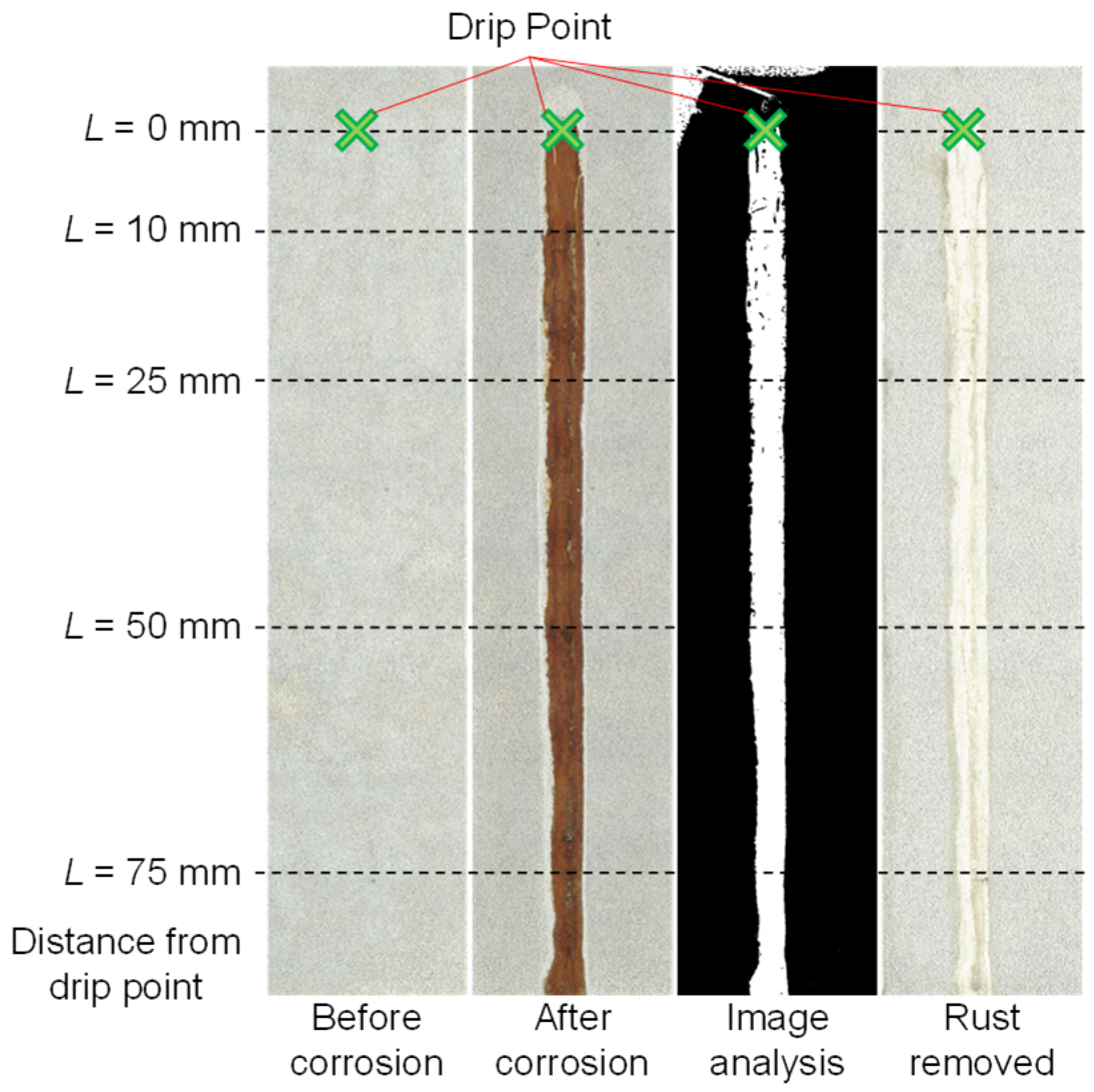
In addition, surface profiles of uncorroded areas were measured before and after rust removal to confirm in advance that any profile change was within the measurement resolution. The specimens were immersed in this solution at room temperature for 30 min, rinsed with distilled water, and dried. This procedure was repeated twice. An example of rust removal using this procedure is shown in Figure 3. Although the comparison in uncorroded areas supported the practical applicability of the present removal protocol, the possibility of local alteration during rust removal in corroded regions cannot be completely excluded.

2.4. Image Analysis and Statistical Analysis

Images captured during the droplet experiments were analyzed using GIMP version 2.10.38. The blue channel, which provided the highest contrast between the rust region and the background, was selected for analysis. After extracting the blue channel using the gimp-drawable threshold function, it was binarized using a rust threshold value of 45. The threshold value was selected to maximize consistency with visual evaluations by multiple experienced observers and was the same in all analyses. The imaging conditions were kept constant throughout all experiments, and stable extraction was achieved using this threshold. The distance along the vertical line from the droplet point was defined as L, and positions at L = 0, 10, 25, 50, and 75 mm were defined as common observation regions in this study (Figure 3). In image analysis, the analysis range was set to 10 mm to the left and right of the intersection of the vertical line and each L position. The rust width within the analysis range was measured in all images, and its temporal evolution was determined. In images where rust was detected, all rust regions were within the analysis range.

2.5. Surface Profile Measurement and Definitions

Surface profiles were obtained using a 3D surface measurement system (VR-3000/VR-3200, KEYENCE Corporation, Osaka, Japan). The system was used under the manufacturer’s routine calibration and inspection condition. Because the system does not provide a user-performed manual calibration function, all measurements were carried out using this maintained instrument condition and consistent settings throughout the study. Position x along the line profile was defined so that the left edge of the detected rust region corresponded to x = 0. The initial profile before droplet supply was defined as $z_0\left(x\right)$, the profile after corrosion under each condition as $z_{\mathrm{c}}\left(x\right)$, and the profile after rust removal as $z_{\mathrm{r}}\left(x\right)$. To minimize the effects of the initial roughness and waviness inherent to each specimen, the postcorrosion profile $z_{\mathrm{c}}\left(x\right)$ and the profile after rust removal $z_{\mathrm{r}}\left(x\right)$ were compared with the initial profile $z_0\left(x\right)$. The differences were calculated using the following expressions.

$$z_{\mathrm{c}}^{\ast }\left(x\right)=z_{\mathrm{c}}\left(x\right)-z_0\left(x\right)$$

(1)

$$z_{\mathrm{r}}^{\ast }\left(x\right)=z_{\mathrm{r}}\left(x\right)-z_0\left(x\right)$$

(2)

These were defined as corrected values—$z_{\mathrm{c}}^{\ast }\left(x\right)$ and $z_{\mathrm{r}}^{\ast }\left(x\right)$, respectively. Furthermore, the rust layer height at position x, $h_{\mathrm{rust}}\left(x\right)$, was calculated from the difference between the corrected profiles. Therefore, the rust-removed surface profile should be interpreted as a relative profile-based morphological metric obtained under the present removal protocol, rather than as a direct absolute measure of corrosion depth. Because porous or loosely adherent rust may affect the measured pre-removal surface profile, the rust layer height evaluated here should be interpreted as a profile-based relative height metric under the present measurement protocol, rather than as a direct absolute measure of porous rust thickness.

$$h_{\mathrm{rust}}\left(x\right)=z_{\mathrm{c}}^{\ast }\left(x\right)-z_{\mathrm{r}}^{\ast }\left(x\right)$$

(3)

Although $z_{\mathrm{r}}^{\ast }\left(x\right)$ may locally exhibit positive values, the sign was retained during analysis as a measured value that indicates variations arising from reference plane definition and measurement resolution. A positive value does not suggest an increase in the amount of metallic material. No unidirectional correction was applied, as it could introduce statistical bias. At each predefined observation position (L), one representative line profile across the rust streak was extracted for analysis. The line profile was discretized at intervals of Δx = 4.2 µm along the x-direction. The analysis was based on line profiles taken across the rust streak (x-direction). Therefore, the evaluation represents variations along this line rather than changes over the entire surface area. The numerical integrations of $z_{\mathrm{r}}^{\ast }\left(x\right)$ and $h_{\mathrm{rust}}\left(x\right)$ were performed by multiplying each value by the pixel width (Δx) and summing along the extracted line profile.

$$S_{\mathrm{r}}=\int z_{\mathrm{r}}^{\ast }\left(x\right) dx$$

(4)

$$S_{\mathrm{rust}}=\int h_{\mathrm{r}\mathrm{u}\mathrm{s}\mathrm{t}}\left(x\right)dx$$

(5)

These integrated values ($S_{\mathrm{r}}$ and $S_{\mathrm{r}\mathrm{u}\mathrm{s}\mathrm{t}}$) represent one-dimensional line-integrated profile metrics for the rust-removed surface profile and the rust layer height, respectively, at each observation position L. They were obtained by integrating the profiles along the x-direction and should not be interpreted as true volumes, mass losses, or area-based damage measures.

3. Results

3.1. Rust Formation Under the Intermittent Supply of NaCl Droplets

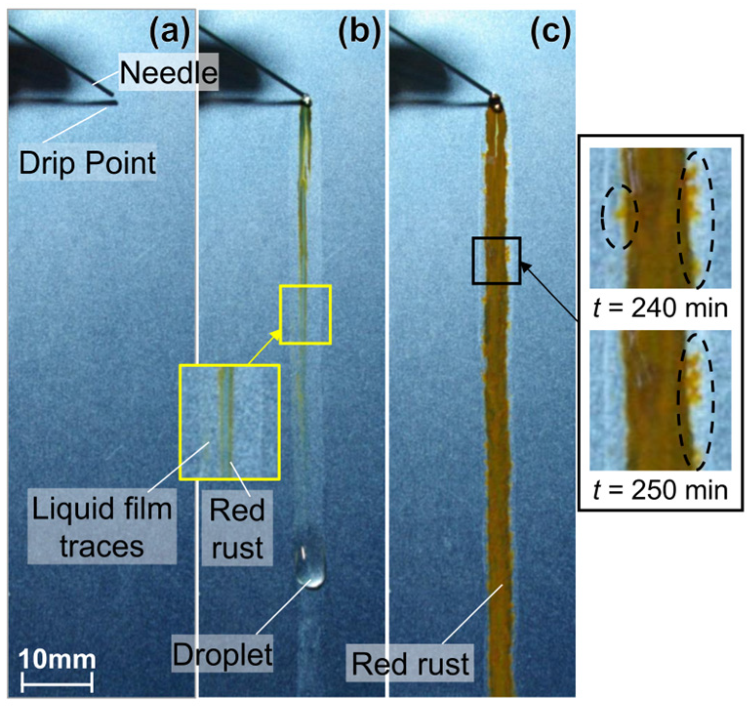
Figure 4 shows the temporal evolution of rust formation under Q = 30 µL/min up to t = 250 min. The right panels in Figure 4c present magnified images of the framed area and the same region 10 min earlier. Before the droplet supply, the surface appears rather smooth. After droplet initiation, red rust was first formed directly beneath the droplet and extended downward along the flow direction. The most upstream point of the rust streak approximately coincides with the droplet impact point. Note that Figure 4 shows images taken during the droplet experiment, whereas Figure 3 corresponds to the specimen state after the completion of the test.

A region paler than the surrounding substrate is observed adjacent to and flanking the red rust. This pale region is distinguishable from the red rust area, and its width is comparable to the droplet diameter shown in Figure 4b. Using a separate specimen, a similar pale region was generated and analyzed using scanning electron microscopy with energy-dispersive X-ray spectroscopy (JSM-6610, JEOL Ltd., Akishima, Japan) after sufficient drying. Sodium was widely detected in this area. In the wet state, the pale appearance of this region was attributed to reflection from the liquid film. In the dried state, it was attributed to diffuse reflection from crystallized sodium chloride and associated salts. Hereafter, this region is referred to as the liquid film trace.

At t = 250 min, a continuous rust streak with a width of approximately 3 mm is observed extending downward from the drip point. Magnified images show rust within the liquid film trace, which appears lighter than the central rust area. This lighter rust deformed and partially disappeared within a short time by undergoing microscale redistribution.

3.2. Temporal Evolution of Rust Streak Width at Different Distances from the Drip Point

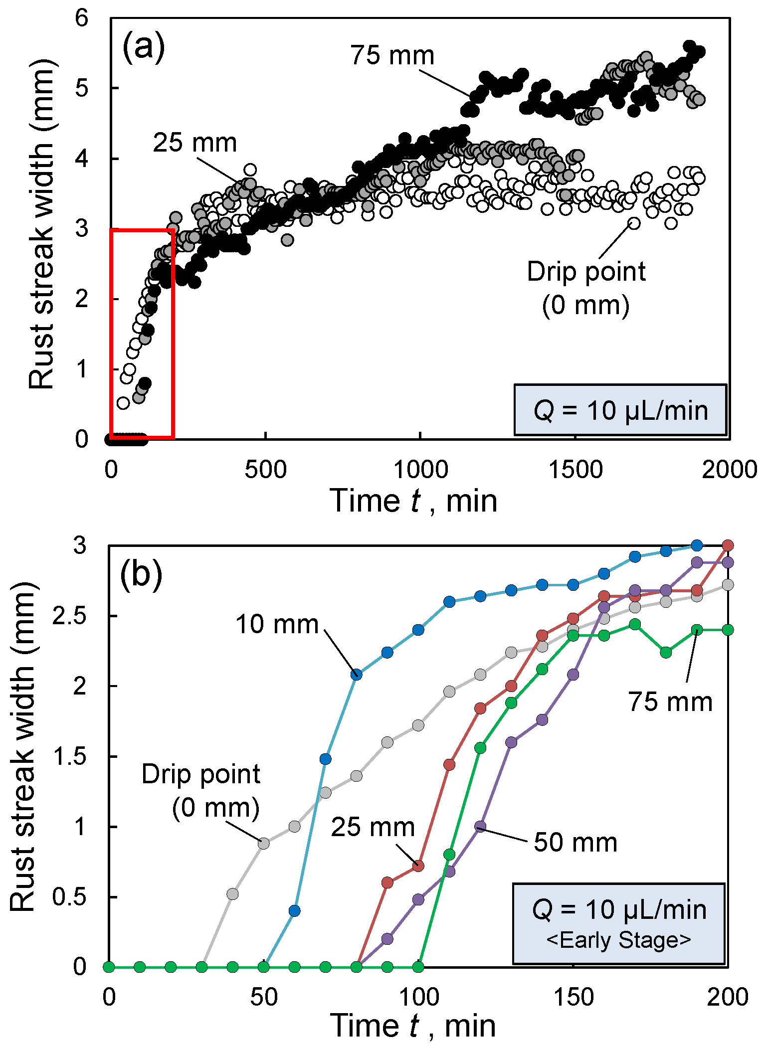
Figure 5a shows the temporal change in rust streak width at L = 0, 25, and 75 mm under Q = 10 µL/min up to 1900 min. Figure 5b presents an enlarged view of the red-boxed region in (a), showing early-stage behavior up to 300 min.

At nearly all observation positions, the width increased within approximately 200 min, reaching about 2.5 mm. Once the width reached approximately 2.5–3.0 mm, the increase became limited. At t = 1900 min, the final width was approximately 4 mm at L = 0 mm and approximately 5 mm at L = 25 and 75 mm. At the drip point (L = 0 mm), the width increased with variations below 1 mm. At L = 25 and 75 mm, the width varied by about 1 mm over several hundred minutes. The small variations observed at the drip point (L = 0 mm) were attributed to minor variations in the liquid-film state (wetting, film thickness, and optical reflection conditions) induced by intermittent droplet supply, whereas those at L = 25 and 75 mm may be associated with the movement of lighter rust observed in Figure 4.

As shown in the enlarged view in Figure 5b, at L = 0 mm, rust was first detected at t = 40 min. Detection time increased with distance: after the first detection at L = 0 mm, detection at downstream positions occurred after a delay. At all positions, the increase in width became limited after reaching approximately 2.5–3.0 mm.

3.3. Effect of Saltwater Supply Rate on the Rust Streak Width

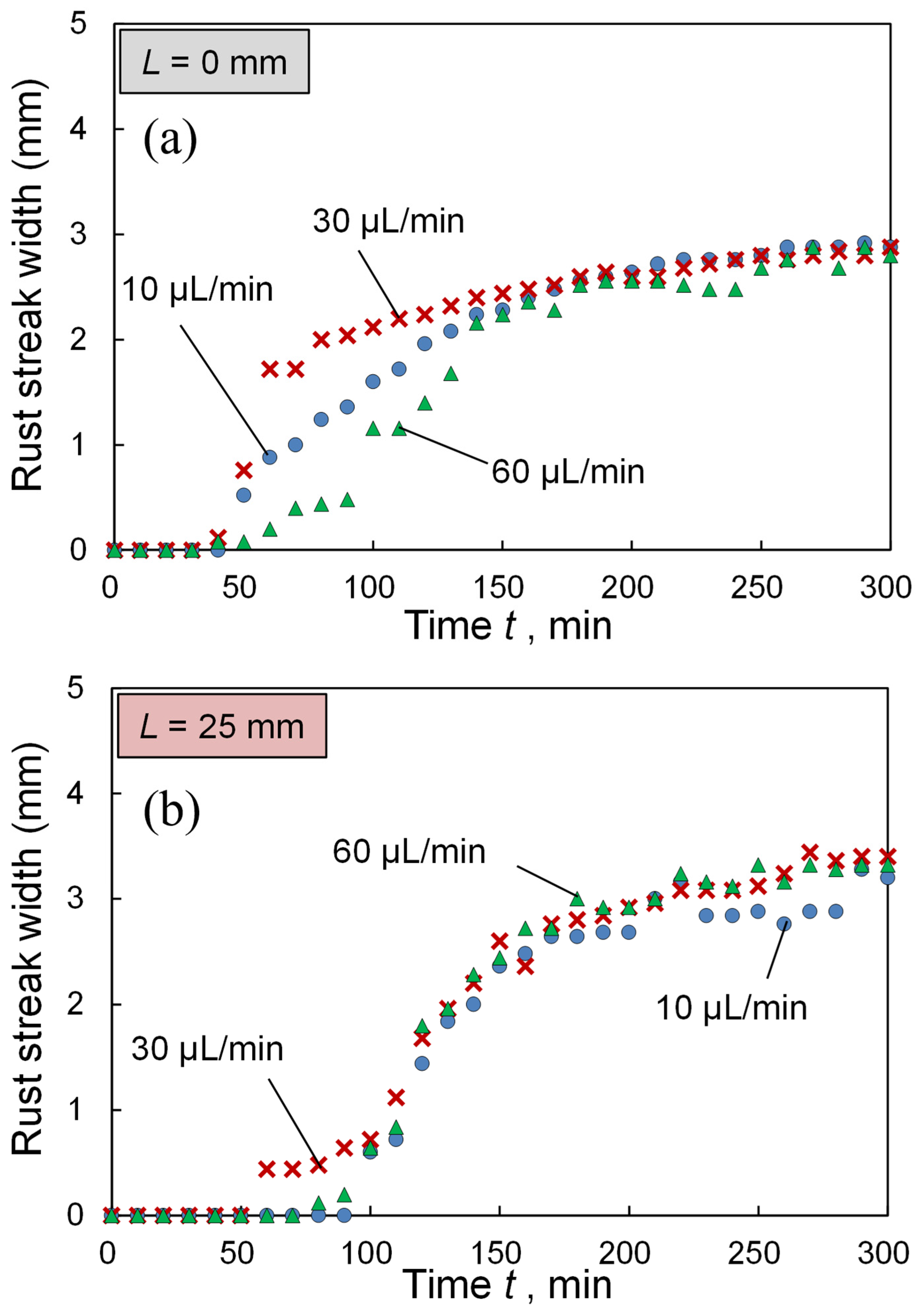
Figure 6 shows the evolution of rust streak width at L = 0 and 25 mm under Q = 10, 30, and 60 µL/min up to 300 min. Here, “rust streak width” is defined as the lateral width of the continuous rust streak formed along the downstream direction from the drip point.

At L = 0 mm, rust first appeared at t = 40 min under all flow rates. Within t = 40–150 min, differences in the expansion rate of the rust streak width are observed among flow rate conditions. At L = 25 mm, under Q = 30 µL/min, larger widths are observed at t = 60–90 min. Outside this interval, no clear difference among flow rates is observed.

3.4. Spatial Distribution of the Rust Layer Height

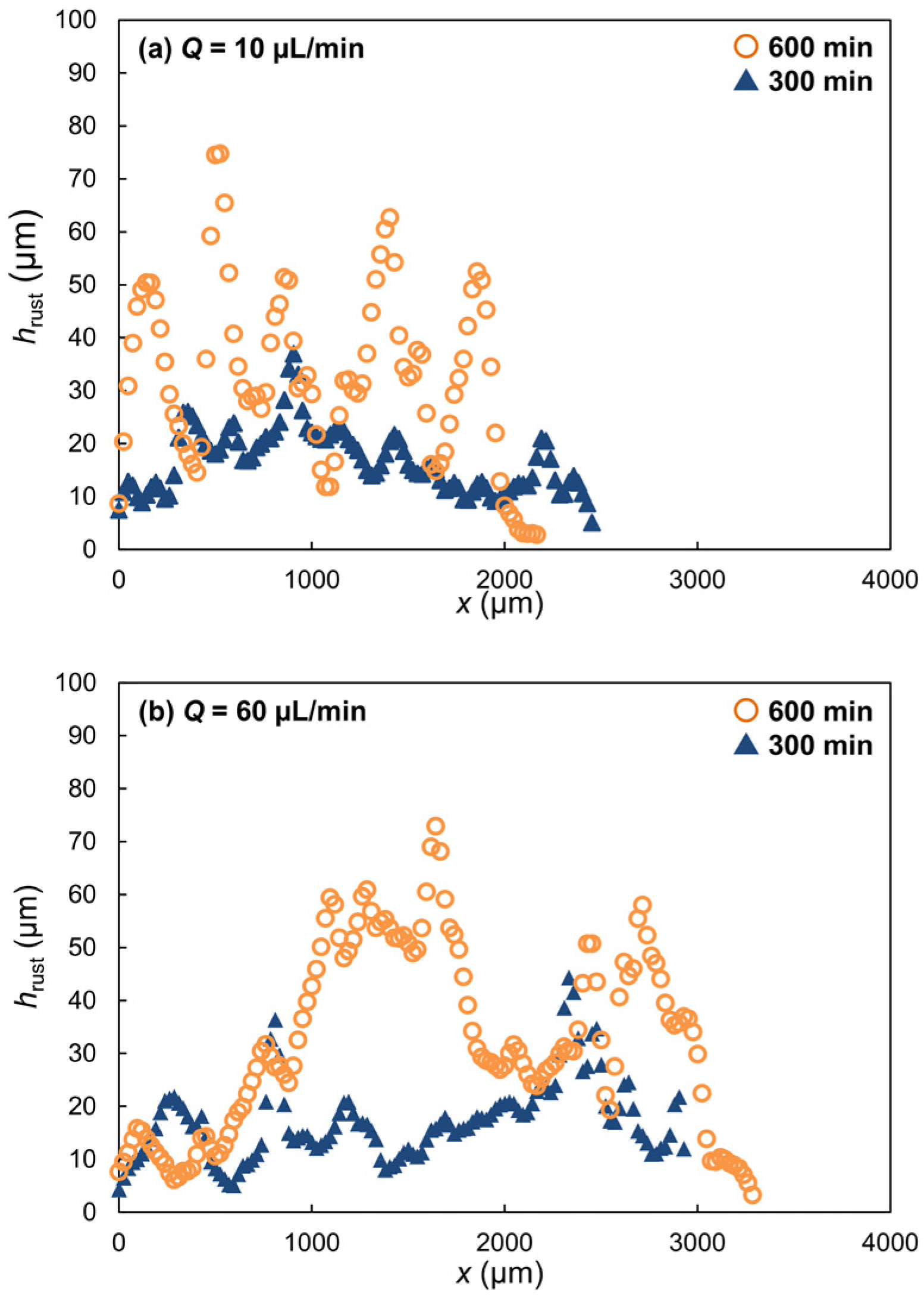
Figure 7 shows the distribution of the rust layer height at L = 75 mm for Q = 10 and 60 µL/min. The 300 and 600 min data were obtained from separate specimens. At both flow rates, the increase in the rust layer height from 300 to 600 min is not uniform over the entire x range. Instead, growth occurs in localized regions.

For Q = 10 µL/min, the integrated rust layer height ($S_{\mathrm{r}\mathrm{u}\mathrm{s}\mathrm{t}}$) was 0.41 × 10⁵ µm² at 300 min and 0.71 × 10⁵ µm² at 600 min. Doubling the exposure time resulted in a 1.7-fold increase in $S_{\mathrm{r}\mathrm{u}\mathrm{s}\mathrm{t}}$.

For Q = 60 µL/min, $S_{\mathrm{r}\mathrm{u}\mathrm{s}\mathrm{t}}$ was 0.51 × 10⁵ µm² at 300 min and 1.07 × 10⁵ µm² at 600 min, representing a 2.1-fold increase. Thus, $S_{\mathrm{r}\mathrm{u}\mathrm{s}\mathrm{t}}$ at the downstream region increased with exposure time and supply rate.

3.5. Comparison of Rust Layer Height and Rust-Removed Surface Profile

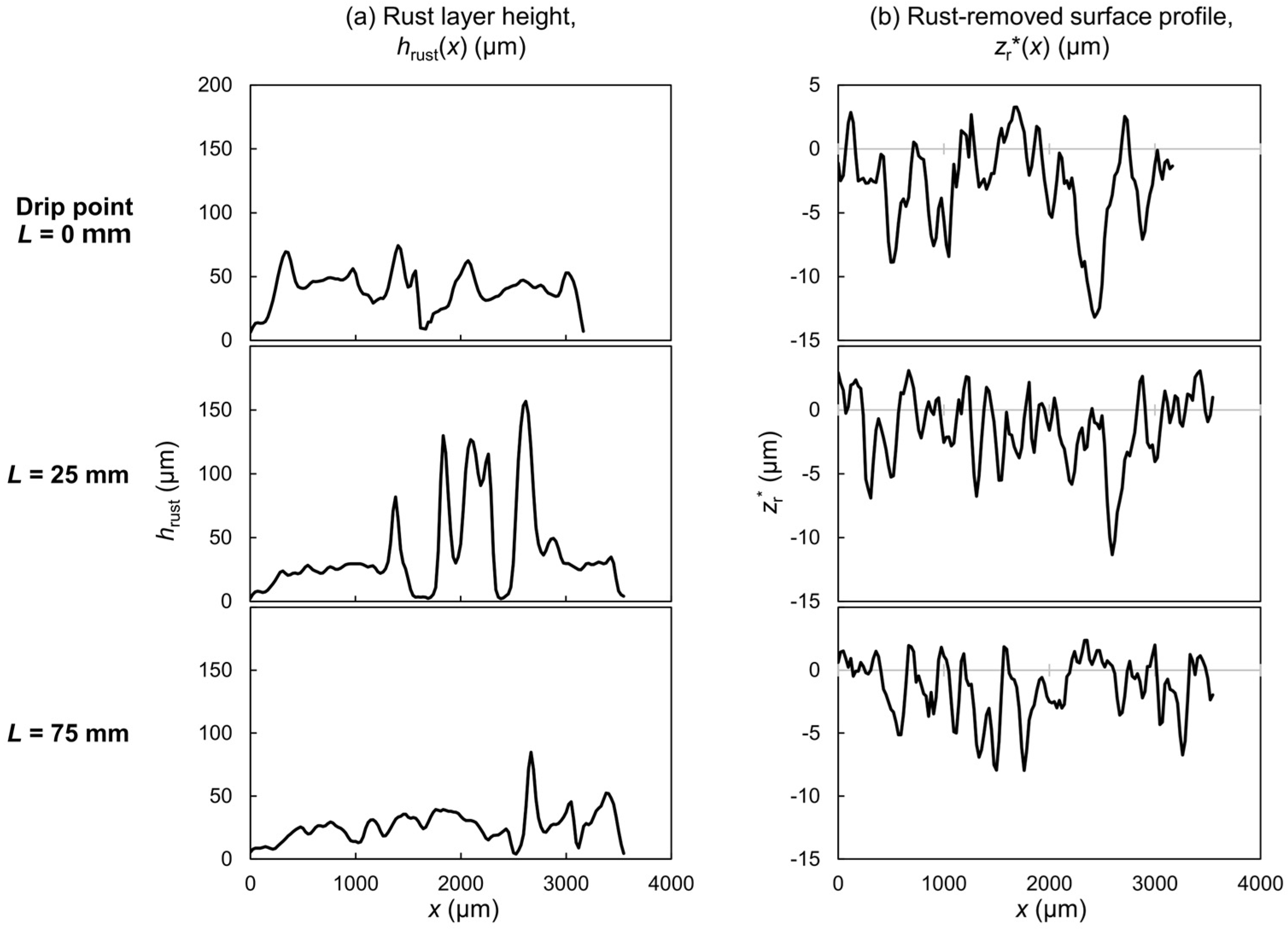
Figure 8 shows the rust layer height ($h_{\mathrm{r}\mathrm{u}\mathrm{s}\mathrm{t}}\left(x\right)$) and rust-removed surface profile $z_{\mathrm{r}}^{\ast }\left(x\right)$ at Q = 30 µL/min and t = 600 min for L = 0, 25, and 75 mm.

At L = 0 and 75 mm, most values of $h_{\mathrm{r}\mathrm{u}\mathrm{s}\mathrm{t}}\left(x\right)$ are below 50 µm. At L = 25 mm, localized regions with $h_{\mathrm{r}\mathrm{u}\mathrm{s}\mathrm{t}}\left(x\right)$ exceeding 100 µm are observed, whereas some areas show $h_{\mathrm{r}\mathrm{u}\mathrm{s}\mathrm{t}}\left(x\right)$ below 10 µm. In contrast, the rust-removed surface profile exhibits no clear differences among L positions. Values are predominantly negative, with occasional positive values. Positive values are below +5 µm and within the range of the initial roughness (R_p = 5.1 µm) and postremoval surface topography (peak-to-trough: 8–9 µm). Because the rust-removed surface profile shows a more complex spatial pattern than the rust layer height, the relationship between the two quantities was further examined using scatter plots.

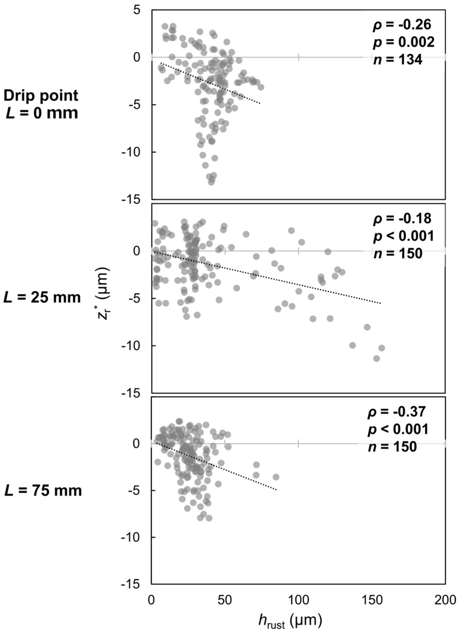
Figure 9 exhibits scatter plots comparing the rust layer height and rust-removed surface profile at L = 0, 25, and 75 mm. At L = 25 mm, the distribution contains a cluster below 20 µm and outliers exceeding 80 µm. Because this distribution is nonnormal, Spearman’s rank correlation coefficient ρ was used as a supplementary indicator.

The number of data points at each location was n = 134 at L = 0 mm, n = 150 at L = 25 mm, and n = 150 at L = 75 mm. Spearman’s rank correlation coefficients are ρ = −0.26 (p = 0.002) at L = 0 mm, ρ = −0.18 (p < 0.001) at L = 25 mm, and ρ = −0.37 (p < 0.001) at L = 75 mm. Although all coefficients are negative, they are small in absolute value. Thus, despite a weak negative tendency, no clear direct relationship was identified between the rust layer height and rust-removed surface profile.

3.6. Integrated Rust Layer Height and Rust-Removed Surface Profile Along the Flow Direction

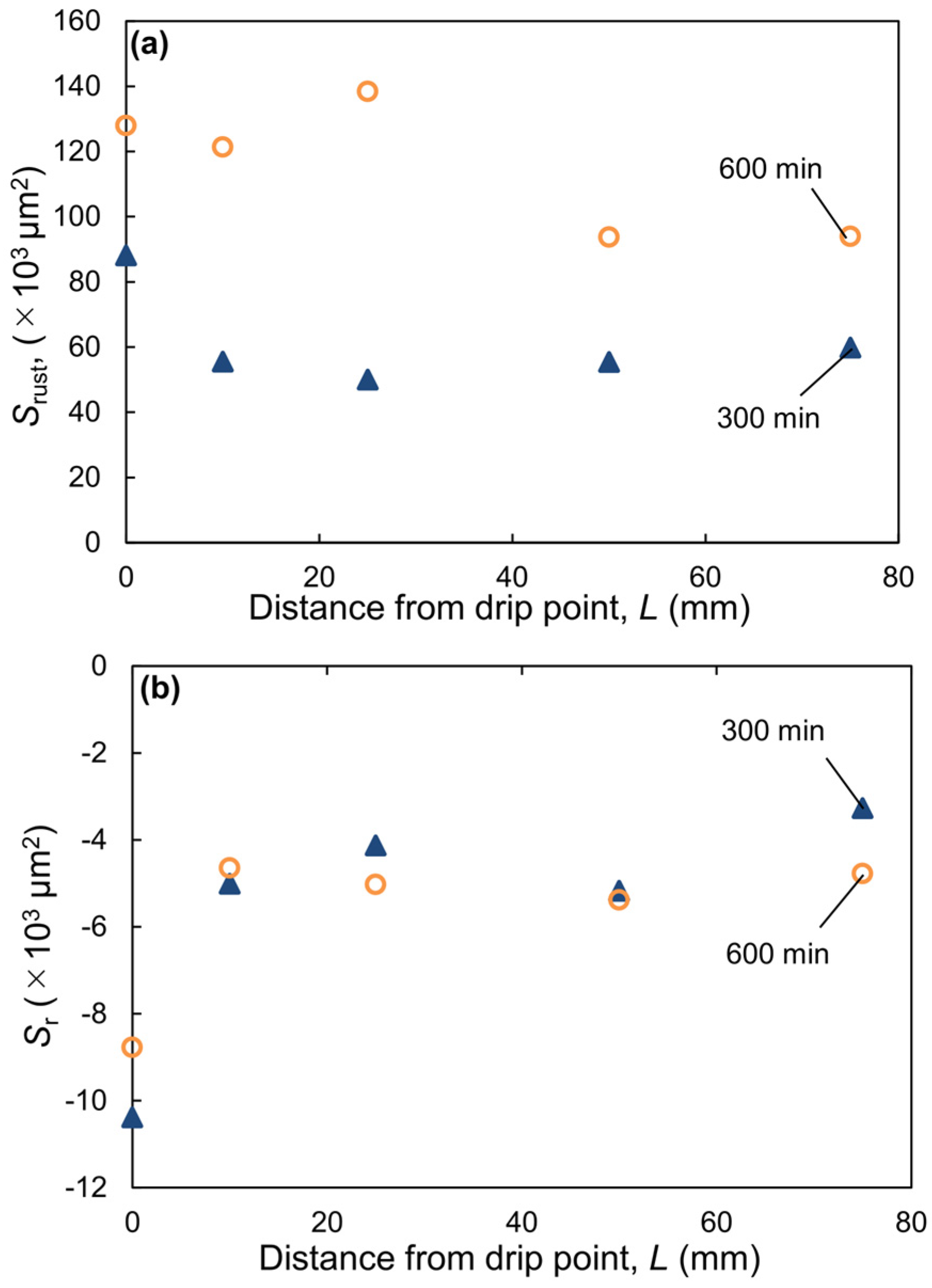
Figure 10 shows the integrated rust layer height ($S_{\mathrm{r}\mathrm{u}\mathrm{s}\mathrm{t}}$) and integrated rust-removed surface profile ($S_{\mathrm{r}}$) at Q = 30 µL/min for t = 300 and 600 min.

Rust layer height increased with exposure time at all positions (L). Integrated rust-removed surface profile values were negative at all positions, indicating a downward shift in the measured rust-removed profile relative to the initial surface under the present removal protocol. In some cases, the 300 and 600 min values of $S_{\mathrm{r}}$ reversed in magnitude. However, the difference was at most approximately 2000 µm². This difference is small compared with changes in rust layer height ($S_{\mathrm{r}\mathrm{u}\mathrm{s}\mathrm{t}}$).

At t = 300 min, the integrated rust layer height ($S_{\mathrm{r}\mathrm{u}\mathrm{s}\mathrm{t}}$) is the largest at L = 0 mm and markedly differs from the values at other positions. At t = 600 min, the differences among $S_{\mathrm{r}\mathrm{u}\mathrm{s}\mathrm{t}}$ values at L ≤ 25 mm became smaller. The magnitude of the integrated rust-removed surface profile at the drip point is approximately twice that at other positions, independent of exposure time.

4. Discussion

4.1. Contributions of Rust Formed at the Same Location and Rust Carried from Upstream

As shown in Figure 4, red rust first formed directly beneath the drip point and then extended downstream along the flow direction. The magnified images show lighter rust moving along the edge of the streak within the liquid film trace. This lighter rust is interpreted as rust carried from upstream. Figure 5b also shows that rust first appeared near the drip point, whereas downstream extension occurred after a delay. In Figure 4b, the light-colored rust in the middle of the downstream extension is therefore also interpreted as rust carried from upstream. These observations indicate that the rust streak contained both locally formed rust and rust carried from upstream. The transported rust contributed first to downstream extension, after which locally formed rust increased the streak width. Figure 7 shows that, after long exposure under the present experimental conditions, the rust layer height is not uniform across the rust streak but exhibits a complex, uneven distribution. This was attributed to the complex deposition pattern of rust carried from upstream. These observations suggest that the rust observed at a given position did not consist only of locally formed rust. These phenomena occurred within the liquid film trace. As the rust width increased, it approached the width of the liquid film trace.

The results in Figure 10 support the above conclusions. At the drip point, there was no effect of rust carried from upstream; therefore, the integrated height of the rust layer increased with time because of local rust formation. The increase in rust layer thickness with the extension of test time is clearly smaller at the drip point than immediately downstream. This is because downstream, the rust carried from upstream was deposited in addition to locally formed rust. Figure 8 shows the distribution of the rust layer height and the distribution of the surface profile after rust removal. The two distributions markedly differ. Figure 9 exhibits scatter plots of the relationship between them. Spearman’s rank correlation coefficient ρ is negative at all positions. However, its absolute values are small, with almost no relationship observed between the two variables. In other words, even where the substrate-side profile change was relatively large, the rust layer was not necessarily thick. This was attributed to the effect of the deposition of rust carried from upstream. Thus, under conditions where droplets flow down the surface, the effect of rust carried from upstream cannot be ignored. This effect is not uniform across different positions.

4.2. Comparison with the Rust Formation Mechanism Under Static Droplet Conditions

The rust formation mechanism caused by a single static droplet has been studied in detail. Previous studies [33,34] have reported that the position where corrosion progresses and the position where corrosion products precipitate and accumulate do not necessarily coincide. Specifically, in a single static droplet, the anodic and cathodic reactions are spatially separated. Oxygen reduction tends to occur at the droplet periphery, including the region near the three-phase boundary. In contrast, metal dissolution tends to occur closer to the center. As a result, corrosion products tend to form and accumulate in the intermediate region between these reaction zones. Therefore, even in a single static droplet, the area where substrate material is lost differs from the area where rust accumulates. It has also been reported that local corrosion behavior within a droplet depends on conditions such as oxygen supply and electrolyte film properties [35,36]. Specifically, in thicker liquid films, it is harder for oxygen from the outside to reach the surface. Therefore, corrosion progresses less readily. In contrast, in moderately thin regions, it is easier for oxygen to reach the surface. Therefore, corrosion progresses more readily in such regions. However, in extremely thin regions, the liquid film becomes unstable. As a result, corrosion may instead become less likely to progress.

In the present study, droplets supplied to the surface flowed down the inclined surface. Earlier droplets first formed a liquid film trace, and later droplets intermittently passed over it. Under such flowing-droplet conditions, corrosion reactions and liquid movement may have proceeded simultaneously within the liquid film. In general corrosion processes, metal dissolution can supply iron ions, oxygen reduction can produce hydroxide ions, and these dissolved components can contribute to the formation of initial corrosion products. Under the present flowing-droplet condition, such corrosion products may have formed locally, moved within the liquid film, become incorporated into the rust streak, and been transported further downstream. This interpretation is consistent with the observed downstream extension of the rust streak and the presence of lighter rust within the liquid film trace. However, the local chemical species, their spatial distributions, rust phases, and porosity were not directly characterized in this study. Moreover, the present results were not directly compared with electrochemical measurements or model-based predictions. Therefore, this discussion should be regarded as a qualitative interpretation consistent with the observed morphological and profile-based results, rather than as direct mechanistic evidence. Detailed characterization of rust phases, porosity, and local chemical distributions, as well as quantitative comparison with electrochemical models, remains an important subject for future study.

4.3. Implications for Corrosion Evaluation

Conventional industrial corrosion evaluation is mainly based on appearance. The results obtained herein suggest the limitations of appearance-based corrosion evaluation under the present liquid-flow condition. Industrial standards such as [37] classify rusted surfaces based on visual appearance; furthermore, some studies [38] have also used appearance as one indicator for comparative corrosion assessment. However, under corrosion conditions involving liquid flow and rust streak formation, such appearance-based assessment does not necessarily reflect substrate-side profile changes observed under the present protocol. In the present study, this limitation was suggested by the relationship between the rust layer height and the rust-removed surface profile. Rust observed at a given position includes both rust formed locally and rust carried from upstream. As a result, in corrosion phenomena accompanied by flowing liquid and rust streak formation, the appearance and substrate-side profile changes should be evaluated separately.

Some studies on corrosion under atmospheric exposure have suggested a correlation between appearance and corrosion progression [39,40]. However, in corrosion that occurs under conditions such as salt spray testing, the flow of attached saltwater droplets down an inclined surface must necessarily be considered. Under such liquid-flow conditions, visible rust includes not only locally formed rust but also rust carried from upstream. Therefore, under such conditions, there is not necessarily a direct relationship between appearance and corrosion progression or between appearance and substrate-side profile change. In particular, this study suggests that rust transport and redeposition may contribute to a mismatch between the apparent rust distribution and the substrate-side profile change observed under the present protocol. Because the present study was based on a limited parameter window and did not include direct physicochemical characterization or model-based validation, the results should be regarded as case-specific morphological observations and as a benchmark for future experimental and modeling studies.

5. Conclusions

(1)

Rust streaks initiated directly beneath the droplet supply point and extended in a streak-like form in the downstream direction. Under the present conditions, the increase in rust width became limited after reaching approximately 2.5–3.0 mm, which is comparable to the droplet diameter.

(2)

In the downstream region, the rust layer height increased with increases in test duration and supply flow rate. In contrast, the integrated rust-removed surface profile was relatively small and did not correspond to the scale of visual expansion.

(3)

Rust layer height and rust-removed surface profile showed only a weak negative tendency and no clear direct relationship.

(4)

Rust streak formation can be understood as a coupled process involving not only localized corrosion reactions but also the transport and redeposition of corrosion products and other dissolved components in the liquid film. The contribution of locally formed rust is greater near the drip point, whereas the contribution of rust carried from upstream increases in downstream regions. This interpretation is consistent with the observed morphology, but the local chemical species, rust phases, porosity, and local pH/ion distributions were not directly characterized in this study.

The present study offers a quantitative methodology that separates rust-streak morphology (e.g., width and spatial distribution) from substrate-side profile changes. These conclusions were obtained under the present experimental conditions, namely SPCC steel, a NaCl concentration of 50 ± 5 g/L, a specimen tilt angle of 70°, flow rates of 10–60 µL/min, and monitored ambient ranges of 15–20 °C and 40–50% RH. The quantitative relationships observed in this study may differ under other material, inclination, solution, flow, or environmental conditions. Therefore, the results obtained herein should be regarded as case-specific morphological observations and as a benchmark for future experimental and modeling studies within the tested parameter window, contributing to an improved understanding of rust-streak-related corrosion phenomena and to the reconsideration of appearance-based evaluation criteria.