Structural Health Monitoring in Historical Buildings: A Network Approach ^†

Abstract

Structural health monitoring (SHM) in historical buildings can be achieved through systems that rely on Wireless Sensor Networks (WSNs). Such systems have the ability to acquire information fast and reliably, making them ideal for SHM applications. Historical buildings, having been exposed to the wear of time, are especially sensitive to any kind of intervention. As a result, keeping them as intact as possible is a critical factor for their integrity. In the current work, a low-cost WSN system and a synchronization algorithm are developed in order to be employed for SHM of historical buildings. The synchronization of WSN-based SHM systems is critical for the collection of accurate information describing the building’s condition. The effectiveness of the assumed hardware and the synchronization algorithm were evaluated with two experiments. The first took place under laboratory conditions and its results showcase the algorithm’s accuracy of synchronization. The second experiment was conducted in a real-world environment. For that purpose, the Ionian Campus Testbed was chosen since it comprises buildings that are more than 200 years old. These buildings are appropriate since they were built with thick stone walls which help determine the system’s effectiveness under such conditions. The results derived from the second experiment showcase the effects of the packet transmission collision avoidance mechanism utilized by the assumed hardware. Finally, an estimation of the average clock skew required for accurate information gathering is derived, based on the materials comprising a historical building.

1. Introduction

Historical buildings play an important role in cultural preservation, and in the extraction of new knowledge about the ways of life and religious beliefs in past times. Structural health monitoring (SHM) [1] systems have gained significant research attention over the last few decades due to relative technological advances. SHM systems can highly contribute to detecting the stability and deformation of a structure and can be employed for the health detection of historical buildings. In particular, sensory devices enhanced with networking capabilities, which enable them to interconnect and exchange valuable information, are the main parts of SHM systems so as to record the necessary information. This information can be derived from active approaches that require an action and measurement process to record the necessary parameters. Such an approach can be an active-sensing acousto-ultrasound-based method [2] which has the ability to record the damage inflicted on a structure. Other approaches include passive methods that can record a structure’s parameters with variable techniques, such as oscillating circuits [3] or accelerometers for ambient vibration detection [4].

Sensory devices have the ability to massively collect information related to environmental attributes of an area or a building where they are deployed. Historical buildings, in particular, are a critical part of many cultures and civilizations worldwide, contributing to a deeper understanding of the way of life and the level of knowledge of ancient times. Obtaining accurate information as quickly as possible regarding the state of a historical building can be a beneficial factor in sufficiently maintaining its integrity [5] and prolonging its lifespan by quickly detecting corrosion inflicted due to naturally occurring phenomena.

Originally, SHM approaches include systems wherein all sensory devices cover their energy needs and communicate using a wired infrastructure [6]. As a result, the system’s price rises due to the materials required for the installation. Many proposed systems [7] use a building’s existing local area network (LAN) cables rather than installing separate infrastructure, thereby minimizing the required cost of materials and installation labor. This showcases that a wired system of sensory devices can collect synchronized measurements with a reliable accuracy for SHM applications. While this approach enables the system to accurately monitor a structure’s condition with minimal time deviations, historical buildings lack a cable infrastructure in most cases, since installing one could potentially pose a threat to its stability and its structural integrity.

On the other hand, wireless sensor networks (WSNs) [8] employ wireless technologies for the communication of the sensory devices. Such systems can operate with minimal intervention to the structure since they do not require cables for their operation. Additionally, they can be installed with minimal alterations to multiple different buildings [9]. The sensory devices (or nodes) of the WSN can be powered by batteries, and they can also acquire a certain amount of energy from ambient environmental sources [10,11]. In addition, WSN systems’ minimal requirements help in minimizing the required cost. Moreover, the minimal installation labor required for such systems provides a level of freedom since the nodes rely on alternative, off-grid sources for their energy demands, while the communications between them employ wireless technologies. Note that these systems are highly utilized for the Internet of Things (IoT) [12] applications, enhancing them with the ability to monitor environmental aspects and provide valuable information.

The quantity and quality of the collected measurements can be determined by two factors: (i) the number of the nodes that collect them; and (ii) the number of measurements in a given time period per node. The quality of the information when measurements are analyzed depends partially on their quantity; thus, larger amounts of them in a given period can benefit the analysis. The analysis of the collected information requires that the measurements are time-correlated. A key factor for the successful operation of WSN-based systems is time synchronization among the nodes in order to collect time-correlated measurements. Synchronized operation of WSN nodes is a challenge given that the nodes operate independently of each other. This independence is caused by their energy sources being autonomous which compels an asynchronous activation of the network. Upon activation, each node initiates time measuring processes using their internal clocks which at that point cannot acquire information from any other clock; thus, the system is not able to obtain time-correlated measurements and derive any useful results.

According to the aforementioned, WSNs require precise clock synchronization to produce accurate results. Historical structures are built with materials [13] (e.g., thick stone walls) that induce variable mechanical properties to the structure itself. These can void the use of high-frequency wireless communications; thus, the WSN nodes will not be able to communicate with the central node (i.e., the node where all data are collected for further analysis) directly in 1-hop transmissions. Collecting as much information as possible, though, requires antennas with high bandwidth and thus higher frequencies. As a consequence, choosing the appropriate hardware for SHM applications in historical buildings is quite a critical part of the system’s development. While higher frequency antennas can provide higher information throughput, the WSN’s nodes lose the ability to communicate directly with each other; thus, a multi-hop network is formed. As a consequence, a synchronization algorithm, which can operate in a multi-hop WSN and accurately synchronize it, is required.

The current work is an extension of [14]. The experiments aimed to evaluate the global clock synchronization performance on the microsecond level and also test the effectiveness of the system during emergency situations (e.g., an earthquake), wherein all nodes are required to simultaneously transmit measurements to a central node for further processing as quickly as possible. The main contribution of the current work is the development of a synchronization algorithm that is able to tackle the communication issues inside historical buildings. The main objective of the synchronization algorithm is to maintain the synchronized measurement collection of the nodes, independently of the clock skew. Additionally, a set of requirements is considered to apply to the discussed objective: (i) the time deviation of the collected measurements should be less than the measurement period so that the measurements collected by different, remote nodes can be all sorted correctly based on the measurement time; (ii) the time deviation of the collected measurements should be less than the time needed for the propagation of wave-like ambient vibrations between a pair of nodes. Moreover, in order to set a threshold for the second requirement, the materials comprising historical buildings and the mechanical properties they introduce to the structure are taken into consideration.

In order to evaluate the effectiveness of the algorithm, two experiments were conducted under variable conditions. The first one was done in a controlled laboratory environment with a small-scale WSN, and the results show that the algorithm can achieve an average synchronization skew of $2000$ μs throughout the network. The second experiment employed a complex of five historical buildings for the WSN installation. These buildings are approximately 200 years old and located near Corfu’s city center. They are comprised of thick stone walls that aid the experimentation process in determining the system’s operation under these conditions. The system comprises a larger-scale WSN. The results show its behavior under emergencies where all nodes are required to simultaneously transmit. In addition, a model that employs the delays of the transmitted packets from all nodes to the central node was developed; it predicts the network congestion during an emergency event.

The results from both experiments showcase that the algorithm can achieve accurate synchronization for the proper operation of the WSN which is considered to be adequate for time-correlated SHM. Precise time-correlated SHM provides valuable information about buildings in real-time but it can also serve for analysis of vibration events. As a result, proper action and informed decisions can be carried out regarding the building’s structural maintenance.

The sections are organized as follows. In Section 2 the related work on synchronization and structural monitoring techniques is presented. Section 3 contains the description of the basic components used to develop the system for the experiments. Next, Section 4 contains the synchronization algorithm developed for the current system. Section 5 includes the experiments conducted for the evaluation of the synchronization algorithm. In Section 6 a discussion on the experimental results is presented and it also covers topics related to the synchronization accuracy and the clock skew for SHM systems in historical structures. In the final Section 7 the conclusions are derived and future work is presented.

2. Past Related Work

SHM in historical buildings requires a certain amount of detail in the detection of a building’s condition [15]. Maintenance requires precise information collection that can be measured with various technological means. These usually measure a building’s symptoms that can be related to a certain condition and proper action can be taken.

De Stefano and Clemente [16], in their study, provide an extensive overview analyzing the problem of SHM from the bottom up since they analyze the main aspects affecting a building’s mechanical and geometrical properties. They also discuss the algorithmic aspects of data analysis, which done right, can potentially aid in deriving more accurate results. Finally, they showcase a sensor network approach and extensively analyze the main functionality of their sensors. Their experiments were conducted in four different historical buildings in Tuscany and Piedmont, Italy.

Earthquake events threaten historical structures, and detecting their condition after such an event is crucial to the proper maintenance. As such, Boscato et al. [17], following the earthquake events of April 2009 that took place in Italy, provide an extensive study and implementation of an SHM system that uses unintrusive monitoring techniques. The historical buildings that are used for monitoring purposes are San Pietro di Coppito and Santa Maria Paganica. The main goal is to determine the mechanical properties of the buildings and provide proper condition detection with both sonic tests and vibrational sensing.

Gattulli et al. [18], in their 2016 study provide an insight into the SHM techniques used in Italy for cultural preservation. More specifically, the showcase mapped areas where SHM systems are installed to serve different purposes such as earthquake detection in masonry buildings. They also point out the main aspects an SHM system requires to successfully monitor a building’s condition.

Pierdicca et al. [19] explored the adoption of WSNs for the detection and mechanical evaluation of historical buildings. The research was done in Italy where historical buildings are especially important to economic prosperity. They developed a WSN that was tested for its monitoring capabilities in Palazzo Comunale di Castelfidardo. The WSN sensors monitor the ambient vibrations of the building to derive an estimate on its condition. Finally, they provide 3D models of the building to visualize the various mechanical properties on different points of the building.

The employment of WSN-based systems has been extensively studied in the literature [20] since they provide potential given the features they incorporate. The data collected from all sensors of the employed system require analysis and precise techniques to derive accurate results about the structural condition of a building [21]. Sadler and Swami [22] provide an extensive overview of the synchronization obstacles faced when developing an algorithm for WSNs. To overcome these, many algorithms have been proposed over the years that incorporate different descriptive network information, as investigated by Lassasme and Conrad in their extensive 2010 survey [23] and by Amulya and Hansdah in a more recent 2015 survey [24].

Elson et al. [25] propose a synchronization technique that uses broadcast transmission as a common point of reference in time. No timestamp is used as a reference clock, but when a node receives a broadcast packet, it retains its local clock as the point of reference. In their work, they propose synchronization algorithms for both single-hop and multi-hop networks. In a 2008 study Noh et al. [26] present a different approach according to which a pair of nodes exchange synchronization messages and neighboring nodes that can hear them can also synchronize their clocks, effectively creating a subset network that is synchronized.

Kim et al. in their work [27] developed and deployed a 46-hop WSN that is used for monitoring the structural health of the Golden Gate Bridge. For the synchronization process, they used the flooding time synchronization protocol (FTSP) and they achieved jitter of less than 10 µs. Their work is based on the paper of Maróti et al. [28] that proposes the FTSP protocol, which uses a broadcast message as the reference transmission for the global synchronization of the wireless network.

Mock et al. [29] propose an algorithm that is based on the synchronization process implemented on the IEEE 802.11 protocol, appropriate for real-time applications on wireless communication networks. The algorithm is based on the master–slave model of operation where the slave nodes synchronize to the master’s clock. Broadcast-based communication is used and a total of two messages are transmitted for the synchronization to take place.

In a 2017 paper, Shi et al. [30] propose a synchronization algorithm that creates a spanning tree from a linear topology suitable for structural health monitoring on bridges. They also employ two algorithms: (i) two-way time message exchange (TTME); and (ii) maximum likelihood estimation (MLE) to determine the clock offset. Finally, they propose a restriction and retry mechanism that helps minimize clock estimation errors from the synchronization, continuous clock offset, and software latencies introduced to the system.

In a 2004 paper, Xu et al. [31] evaluate the Wisden WSN that incorporates a synchronization algorithm and is a structural health monitoring system. Wisden provides reliable, time-correlated structural ambient vibrations measurements from the different nodes in the network. The system provides low-overhead data timestamping on a per-hop basis with no need for global clock synchronization.

Wang et al. [32] in their study published in 2007 propose a synchronization algorithm that employs the point-to-multipoint capability of the transceiver they used for their experiments. The server sends a beacon that can be received from all nodes which get synchronized according to the server’s clock. This synchronization algorithm is part of a system used for SHM.

Shannon et al. in their work [33] propose an extension to the flooding time synchronization protocol. This protocol helps the WSN conserve energy and improves the synchronization accuracy by dynamically optimizing the packet exchange procedure between the nodes with no need for pre-configured transmission intervals.

Su and Akyldiz [34] in their 2005 work propose the time-diffusion synchronization protocol that is used for WSNs. According to their study, the protocol can be used to synchronize all nodes in the network. The network reaches an equilibrium time and the deviations have a small tolerance level. The algorithm uses the master–slave model. The master receives the slave’s timer and a correction is applied on a per-hop basis on the timestamped measurement.

Ganeriwal et al. [35] propose a synchronization algorithm that can work on multi-hop WSNs. All network nodes use the clock transmitted by the initiator node. The experiments, which were conducted using a small real-life WSN system, showed that the average accuracy is less than 20 µs. Simulations were also conducted that verified the synchronization accuracy on larger-scale networks.

Sommer and Roger in their work from 2009 [36] propose a decentralized WSN synchronization algorithm called gradient time synchronization protocol. According to their method, each node broadcasts its clock information at a given interval to their neighbors that in turn use it to calculate the logical clock. There is no need for global clock synchronization; that is especially important in situations in which nodes stop operating.

Li and Rus in their 2006 work [37] discuss four approaches for global time synchronization in WSNs, a node-based approach, a hierarchical cluster-based method, a diffusion-based method, and a fault-tolerant diffusion-based method. Santashil et al. [38] propose an adaptive synchronization algorithm for WSN applications. The synchronization is executed on a peer-to-peer basis that achieves a high precision with minimal resource requirements from the nodes.

Phanish et al. [39] describe the development of a low-cost WSN for SHM at Bobby Dodd Stadium at Georgia Tech. Their approach to the synchronization of WSN requires no GPS or Internet connectivity to be achieved. The algorithm creates a total of three timestamps in order to accurately determine the measurement time. The algorithm has an accuracy of 200 to 300 µs with 95% confidence.

Chen et al. in their 2016 paper [40] developed a synchronization algorithm that is based on event-triggered communications. According to the algorithm, when certain conditions are met each node broadcasts its virtual local clock rates to the neighboring nodes. The algorithm is distributed and does not require information such as the network’s topology.

Fanarioti et al. [41] propose a MAC-layer timestamping algorithm on each measurement during the propagation of the data packets, through a predefined path, to the sink node. Each time a message is transmitted to the route’s subsequent node, and a clock correction is applied locally on the receiver node. This algorithm is used in the current work for determining the clock deviations on all nodes of the network without using a common event that triggers them to calculate a timestamp.

Casarin et al. [42] studied the effects of employing monitoring systems for the structural health assessments of cultural heritage buildings. They also investigated the early warning procedures for emergencies (e.g., earthquakes) that such systems can deliver by continuously monitoring the condition of a structure. Orenday-Tapia et al. [13] in a 2018 study describe a system of non-intrusive nature for collecting information related to the composition and the mechanical properties of the basic materials comprising cultural heritage buildings. They also derive results on wave propagation attributes (e.g., speed, velocity) of ambient vibrations on such buildings.

The current work is an extension of [14], wherein a MAC-layer global clock synchronization based on broadcast transmissions was developed. In the current work, the experiments have been extended in order to evaluate the effectiveness of the synchronization algorithm under real-world conditions. Additionally, the system’s functionality has been adjusted to collect information about its operation under stressful conditions, such as earthquakes.

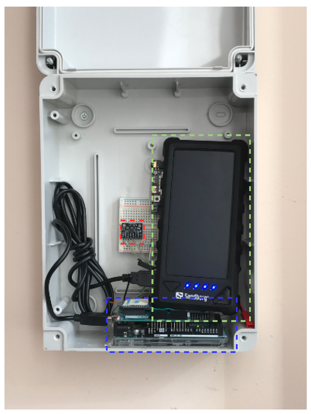
3. System Definition

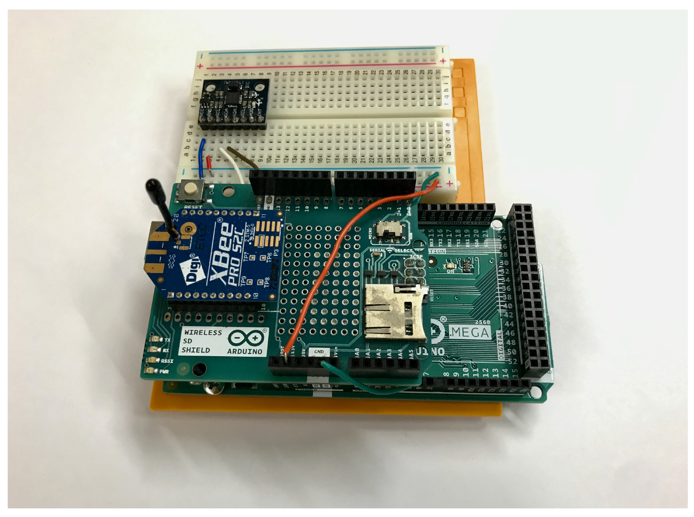
The system is a WSN that comprises materials that incorporate adequate computational power and bandwidth to meet the requirements of SHM applications while maintaining a low cost of implementation and operation. The system is deployed indoors as it is then safer than an outdoor one (e.g., against thieves, extreme weather conditions), but as a result, communication among the nodes becomes increasingly hard due to the basic materials of the structure (e.g., walls). Given the previous communication obstacles (i.e., presence of structural elements such as walls) between communicating nodes, a factor affecting their communication is the antennas and their operating frequency. Lower frequency antennas (e.g., 433 MHz) can achieve more accurate communications inside buildings but they have a lower bandwidth compared to higher frequency ones (e.g., 2.4 GHz). SHM applications require a higher bandwidth, thereby making high-frequency antennas a more appropriate choice for the current application. According to the aforementioned, the XBee RF module was selected for the node’s communication. As such, the system consists of four main parts: (i) the main Arduino board; (ii) a wireless SD Shield; (iii) a Digi XBee RF Module; and (iv) an accelerometer.

3.1. Arduino

The mainboard that handles all the computational needs of a node is the Arduino Mega 2560 Rev3 [43]. The micro-controller contained within the board is an ATmega2560 clocked at 16 MHz. In addition, it includes (i) 256 KB of flash memory; (ii) non-volatile memory used to store the developed code; and (iii) 8 KB of SRAM (volatile memory) that stores local information during the execution of the code.

3.2. Wireless SD Shield

The Arduino board does not support a direct interface for wireless modules. Therefore, a wireless shield [44] is used as an intermediary between the mainboard and the Digi XBee RF Module. The shield connects on top of the Arduino, extending most of the pins, while it also includes a switch that allows the wireless module to communicate with either the USB-to-serial converter or the microcontroller.

3.3. XBee Modules

The Digi XBee RF Module [45] connects on top of the wireless shield and creates an interface between them. The wireless module operates under the ZigBee protocol which is based on the IEEE 802.15.4 standard. The protocol includes three layers: (i) physical; (ii) MAC; and (iii) network. The main capabilities include the routing of data packets in remote nodes of the network and address resolution. The operating frequency of the antenna is between 2.4 and 2.5 GHz, and it can either operate as a coordinator or a router. The coordinator is of vital importance for the establishment of a network comprised of XBee Modules because it is responsible for setting all the network’s parameters, including the PAN ID and the channel to be used. Only one coordinator can exist under the same PAN ID, while in the current application it is also used as the central node (i.e., it gathers the information from all router nodes in the network). The rest of the nodes are set to function as routers. The module is set to operate in Application Programming Interface 2 (API2) mode, allowing each node to gain access to information related to the sender of a packet, and it can also easily route data packets to a specific node inside the network.

ZigBee employs the appropriate packet transmission mechanisms in order to minimize failed ones. More specifically, it operates under the carrier sense multiple access/collision avoidance (CSMA/CA) protocol, according to which a node that has a packet for transmission first senses the physical medium (in this case the air) for active transmissions to avoid overlapping ones. If the medium is available it transmits the packet; otherwise, it calculates a random time instance at which it retries the above steps. The ZigBee protocol has a maximum number of retries equal to three (3).

The XBee-Arduino library [46] handles the communications between the main Arduino board and the XBee antenna. It can also be used for controlling and configuring the XBee antenna. When the antenna receives a data packet from the Arduino board, its installed operating system handles the ZigBee protocol operations. This means that there is no control over the packet transmission through the air. The ZigBee protocol does not provide access to information related to the CSMA/CA protocol’s number of retries for particular packet transmission. Additionally, the number of retries on CSMA/CA by default is set to a maximum of three (3).

3.4. Accelerometer

The accelerometer is a sensor able to measure ambient vibrations of the materials. The accelerometer used for the proposed system (i.e., MPU-6050 [47]) is a low-cost device that boasts decent measurement speed (i.e., 1 every 4 $\mathsf{\mu }$s) and has the ability to measure ambient vibrations with an accuracy of 16-bits. The sensitivity of the module can be set to one of the four (4) different values 2, 4, 8, or 16 g. The sensor also includes an internal processing unit that can potentially execute calculations on the measurements before transmitting them back to the main Arduino board.

3.5. WSN Node

The WSN consists of the assembled nodes. An assembled node is depicted in Figure 1. All WSN nodes transmit the necessary information back to a central node, hereafter referred to as initiator. The data packet includes the information depicted in Figure 2. Packet type is required for the nodes that receive the packet to identify it and take the necessary actions. Next, the measure ID is an integer that keeps count of the number of measurements collected from each node. The timestamp shows the time of measurement calculated using the local clock of the node that created it. Acc. measure is the ambient vibration measurement collected from the node’s accelerometer. Finally, the node ID is the identifier each node has, which is used to show the current vibrational state of a particular place of the structure where the node is installed.

Figure 2 also depicts an example of a packet that the initiator receives during the measurement collection (i.e., the Figure’s bottom part). The information is read as follows: The initiator upon receiving a packet first, the first field, 2, which corresponds to the packet type in order to determine the type of information that is contained inside the rest of the packet. Next, the initiator knows which node created the measurement information by checking the last field, in this case, it is node number 5. The initiator knows that node 5 collected the measurement at time 4,869,390 (in milliseconds) and that this measurement is the 1500th that has been collected. Finally, the accelerometer measurement (which is the result of euclidean distance calculated using measurements for three axes, x, y, and z from within the accelerometer sensors) is equal to 4637.

4. Synchronization of the WSN

The purpose of the node synchronization is to create a globally synchronized virtual clock on WSNs that will later be exploited for timestamping the collected measurements. The following subsections describe the proposed synchronization model and the algorithm that is employed for the final system.

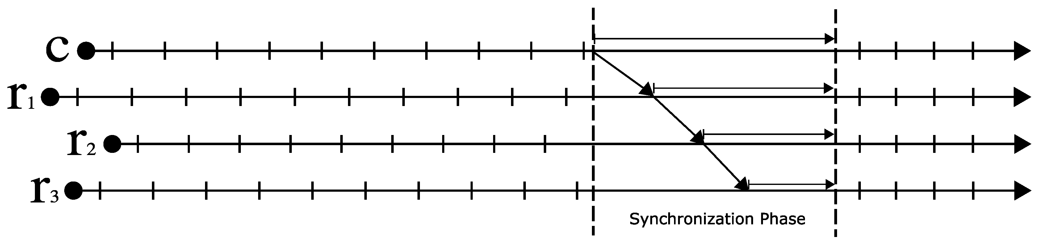
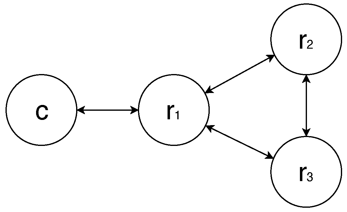
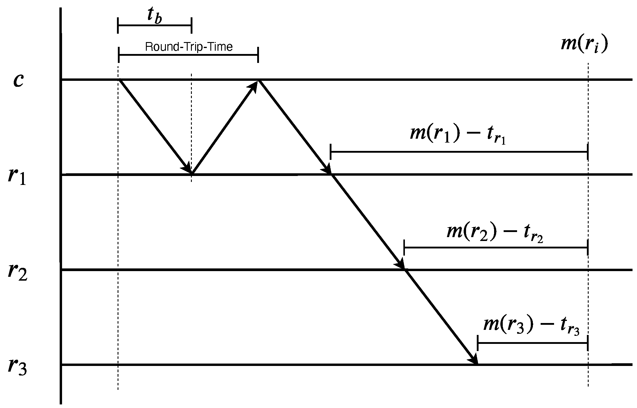
4.1. Synchronization Model

The algorithmic model aims to operate in WSNs with variable attributes (e.g., initiator’s eccentricity, network diameter, network density). In Figure 3, a WSN containing four nodes in chain topology is depicted. The nodes communicate using wireless antennas which provide flexibility for their physical installation procedure. The main issue introduced by such systems is the necessity for time-correlated measurements, as due to the wireless nature of the system all nodes are activated asynchronously. As a result, the collected measurements will not be time-correlated (Figure 3, WSN before synchronization).

4.2. The Synchronization Algorithm

In order for the algorithm to be able to operate in WSNs with different topologies that involve variable attributes, the proposed algorithm takes advantage of information related to these attributes. The algorithm has two distinct phases. During the first phase, the initiator begins a broadcast transmission and retains its current clock $t_s$. The neighboring nodes that receive it retransmit the same packet. Upon delivery to the initiator, another timer $t_e$ is measured. Next, the initiator calculates the round-trip-time $t_e-t_s$ and the end-to-end time:

$$t_b=\frac{t_e-t_s}{2}.$$

(1)

This process extracts preliminary information for the accurate synchronization of the WSN. In order to minimize the complexity of the algorithm, the process is executed once and the acquired information ($t_b$) is used for the second phase.

When synchronization is applied to multiple WSN nodes, time calculation drift is accumulated between the nodes’ clocks after a certain amount of time. Phase two of the algorithm is applied multiple times during the WSN operation to minimize the clock drifts. During this phase, the initiator prepares and encapsulates all the necessary information inside a data packet ready to be transmitted. This includes the initiator’s local timer $t_c$, which is measured right before the transmission takes place, the transmission time $t_b$ calculated on phase one, and a variable $h_{r_i}$ that counts the number of retransmissions the packet is subjected to before it reaches a node $r_i$. Then the initiator broadcasts the packet. When a node $r_i$ receives the packet it retains its local time $t_{r_i}$, updates the $h_{r_i}$ counter, and rebroadcasts the packet. Next it calculates the local time difference $\Delta t_{r_i}$ from the included initiator timer $t_c$ according to Equation (2).

$$\Delta t_{r_i}=t_{r_i}-(t_c+t_b\times h_{r_i}).$$

(2)

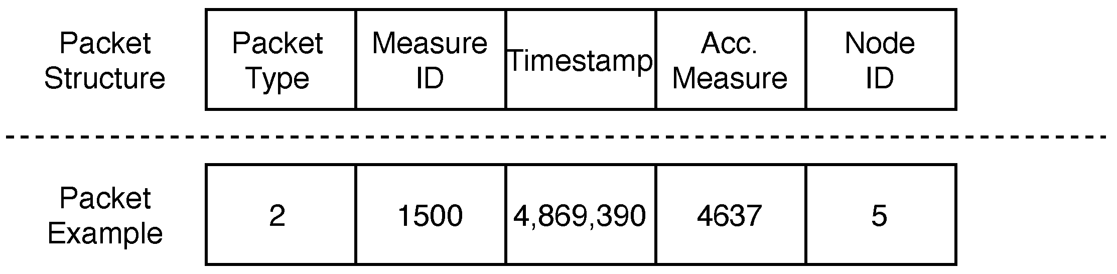
4.3. Synchronized Measurement Initialization

The synchronization algorithm, as described above, creates a global virtual clock for the WSN. One way to start measurements in all nodes of the network is to set a specific time in the global clock, at which all nodes will initiate the measurement procedure at a given interval. Because of variations in synchronization accuracy, inaccurate timestamped measurements may be created, not following the network’s global clock. The synchronized measurement starting time procedure is meant to minimize the effect of inaccurately synchronized nodes in the network. The process requires the initiator’s eccentricity that is collected during the network initialization procedure. First, the initiator calculates its eccentricity, hereafter referred to as e, using the flooding mechanism. More specifically, a broadcast transmission takes place by the initiator including a counter $h_{r_i}$ that tracks the current packet’s hops before it is received by a node $r_i$. Upon receiving it, node $r_i$ updates the $h_{r_i}$ counter and retains this number as its distance in hops from the initiator. Since the eccentricity procedure is based on broadcast transmissions, the nodes $r_i$ might receive multiple packets. In this case, the nodes update the packet’s counter $h_{r_i}$ and check whether it is smaller than the counter from the previously received transmission, and retain the smaller one. This effectively helps calculate the shortest path from the initiator to all nodes. The final step of the eccentricity calculation procedure is the distance request procedure. The initiator requests from all nodes their calculated distance and it retains the greatest distance as the eccentricity e.

In the initial development of the measurement start time equation, the calculations involved a simple scheme that used the initiator’s eccentricity e, the broadcast transmission time $t_b$, and the packet’s hops $h_{r_i}$:

$$m\left(r_i\right)=t_{r_i}+t_b\times (e-h_{r_i}).$$

(3)

With this equation, each node calculates the first measurement time according to its local clock. It is worth mentioning that each node $r_i$ uses a constant number, e, and subtracts the packet’s hop. The result is multiplied with the estimation of the broadcast transmission time, effectively allowing each node to start the measurements with the appropriate delay.

The algorithm is adjusted to reflect the requirements of random topology WSN. The basic scheme that enables all nodes to calculate the measurement start time in proportion to the $h_{r_i}$ counter is retained. Additionally, a statically defined guard period, g, is calculated by all nodes. This period is used to overcome the inaccuracies in the measurements starting after the calculations, introduced by calculation time variability on each node’s processing unit. The guard period is especially important since it allows all nodes to finish their calculations before the measurements are initiated by the WSN. The modified scheme is presented in Equation (4). The measurement start time is calculated upon the network synchronization right after the $\Delta t_{r_i}$ calculation. Note that the e value is multiplied by two since a node $r_i$ can receive a synchronization packet that has traveled more times than the initiator’s eccentricity.

$$m\left(r_i\right)=t_{r_i}+t_b\times (2\times e-h_{r_i})+g.$$

(4)

Figure 4, depicts all the theoretical steps described in the current section of the system’s main operations. $m_{r_i}$ is the time calculated by all router nodes as the measurement initiation time. $m_{r_i}-t_{r_i}$ represents the time each node has to wait before collecting the initial measurement.

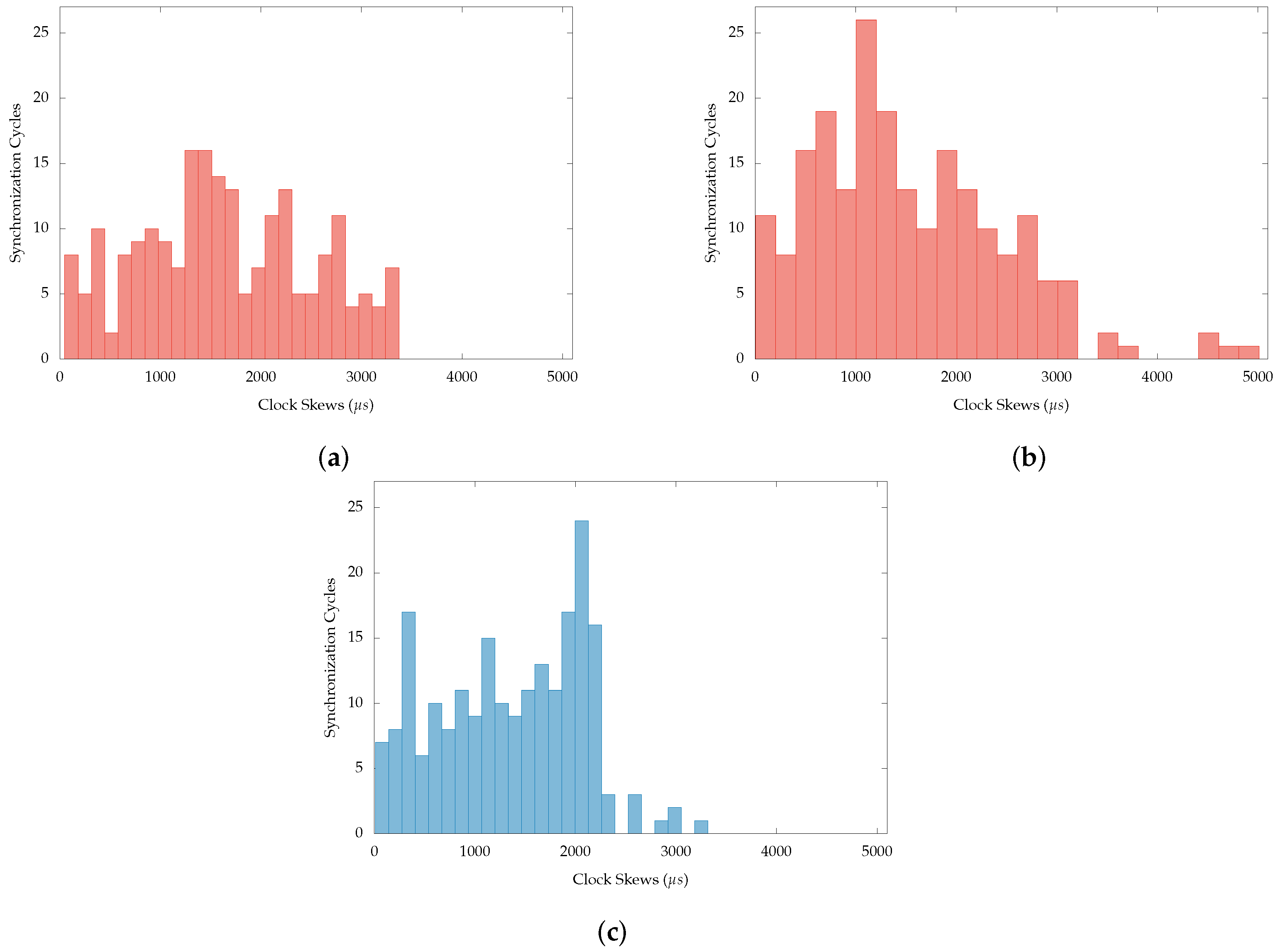
5. Experiments and Results

To evaluate the accuracy of the synchronization algorithm, two experiments were conducted. The first experiment described in Section 5.1 used code execution interrupt events. It was conducted under laboratory conditions using a small-scale WSN that helps evaluate the correctness of the approach. The second experiment described in Section 5.2 was conducted on an already deployed WSN in the two-century-old buildings of the Ionian University Campus [48] and it used the global clock synchronization algorithm described in Section 4 and the per-hop-basis timestamping algorithm [41] to evaluate the synchronization performance. Both experiments used custom-designed software that was developed to function on Arduino boards. The materials comprising both WSNs are described in Section 3.

5.1. Multiple Synchronizations and Interrupt Events

This experiment aims to evaluate the accuracy that can be achieved by the synchronization algorithm described in Section 4. The developed WSN comprises three nodes that are based on the hardware described above. For the experiment, custom-designed code based on the Arduino board was designed. The experiment aimed to evaluate the accuracy of the synchronization algorithm, and for that timestamped events are required. In order for all nodes to measure a timestamp simultaneously, a common event that can be sensed by all of them needs to be created. All nodes of the WSN during the experiments are in a common space and they can communicate directly with each other. The WSN topology is created manually, which means that while the nodes are able to communicate with all others, they are programmed to ignore transmissions from certain nodes, effectively creating the desired topology, depicted in Figure 5.

The Arduino board serially executes the installed code with parts of the instructions having to be iterated. Every node of the WSN needs to execute multiple operations during each loop and their serial execution creates a delay at the microsecond level before any of them can be executed once more. To minimize the delays this effect creates, code execution interrupt events are employed. This Arduino function requires a physical connection to a common cable on all nodes of the WSN. This cable is used to transfer an electrical signal to all of them, consequently creating a code execution interrupt event. This event stops the serial code execution and runs a preset function. When the execution of the function is over, the Arduino board resumes the program’s execution from its previous state.

The developed code causes the following actions: (i) the initiator synchronizes the WSN; (ii) the initiator creates an interrupt event; (iii) the router nodes measure a timestamp according to the globally synchronized clock; and (iv) the router nodes transmit the timestamp to the initiator. The above actions are executed multiple times during the experiment with an interval of 50 s. A total of 213 synchronization cycles are executed during the experiment.

Figure 6 contains the clock skewing right after the synchronization of the WSN’s router nodes combined in one figure. The results show that the mean clock skew achieved by the WSN is equal to 1502 $\mathsf{\mu }$s with a minimum value of 4 $\mathsf{\mu }$s and a maximum of 5012 $\mathsf{\mu }$s. It was observed that the synchronization algorithm can synchronize the nodes with a skew of around 2000 $\mathsf{\mu }$s. More specifically, it was observed that 75% of the skews measured during the experiment were less than 2088 $\mathsf{\mu }$s while the peak of values (63 out of 638 skews) in Figure 6 were between 2100 $\mathsf{\mu }$s and 2300 $\mathsf{\mu }\mathrm{s}$. Finally, it was observed that only seven out of a total of 638 skews measured had values greater than 3500 $\mathsf{\mu }\mathrm{s}$.

Figure 7 comprises three subfigures. These contain the clock skews of every node $r_i$ separately, measured during the experiment. The first two in red represent the router nodes $r_2$ (Figure 7a) and $r_3$ (Figure 7a) that are two hops away ($h_{r_2}=2$ and $h_{r_3}=2$) from the initiator and the blue one represents $r_1$ (Figure 7c) where $h_{r_1}=1$. In Figure 7a it is observed that the measured clock skews vary between 48 $\mathsf{\mu }\mathrm{s}$ and 3372 $\mathsf{\mu }$s. Additionally, 75% of them are equal or less than 2256 $\mathsf{\mu }\mathrm{s}$. The mean value is 1635 $\mathsf{\mu }$s. Figure 7b contains the clock skews of node $r_3$. The mean clock skew measured is equal to 1520 $\mathsf{\mu }$s and it ranges between 4 $\mathsf{\mu }$s and 5012 $\mathsf{\mu }$s. A full 75% of the clock skews are contained under 2100 $\mathsf{\mu }$s and the mean value is 1520 $\mathsf{\mu }$s. Finally, Figure 7c presents the measured clock skews from node $r_1$. They range between 10 $\mathsf{\mu }$s and 3318 $\mathsf{\mu }$s with a mean value of 1345 $\mathsf{\mu }$s. From all measured clock skews, 75% of them were lower than 1980 $\mathsf{\mu }$s.

From the experiment, it was observed that the synchronization algorithm can achieve smaller clock skews on nodes whose distance in hops is greater than other nodes in some cases. More specifically, node $r_3$ (where $h_{r_2}=2$) achieved a synchronization of $4$ μs during the 5th cycle where node $r_1$ ($h_{r_1}=1$) synchronized with a clock skew of 386 $\mathsf{\mu }\mathrm{s}$. This behavior was present since the XBee modules transmit packets based on the CSMA/CA protocol detailed in Section 3. Additionally, the synchronization algorithm uses a static transmission time that is calculated (estimated) upon phase 1. This time is then used for all transmissions related to the synchronization of the WSN (phase 2) which may differ from hop to hop, since each transmission time depends on when the XBee module will sense that the channel is available to initiate a transmission. This behavior is observed in 61.9% of the synchronization cycles.

The final results from the current experiment show the behavior of the synchronization algorithm under the limitations introduced by the basic operation of the ZigBee protocol. For the analysis, a network consisting of four nodes organized in chain topology is considered. Figure 8 depicts the network layout. The ZigBee protocol is based on IEEE 802.15.4 which employs collision avoidance mechanisms such as CSMA/CA. This states that for each attempted transmission from an XBee antenna first listen for active transmissions in the air and tries again at random in the case there is one. The antenna is set to try three times and if it fails on all of them it aborts the transmission. Additionally, the ZigBee protocol states that each broadcast packet is transmitted three times to minimize the possibility that a neighboring node has not received it. In the case of the synchronization algorithm, the facets analyzed above introduce a level of uncertainty for the real transmission time, denoted by $t_b$, where b represents broadcast.

For the synchronization algorithm, as described in Section 4, upon the first phase the initiator derives an estimation of the broadcast transmission time based on the round-trip-time procedure. As explained above, upon the first phase of the synchronization the initiator transmits a broadcast packet. This phase can be divided into two distinct processes. The first one is when the transmission reaches all neighboring nodes which receive the packet and process it. Note that there is no guarantee by the operations of the antennas that all nodes will receive the first of the three broadcast transmissions. The second process is when these nodes, operating under the CSMA/CA protocol, begin the transmission procedure. Upon this, all nodes compete against each other for a chance to transmit the packet. The first node that happens to find the channel available transmits the packet. Taking into consideration the fact that each broadcast transmission is sent three times, it is not possible to obtain knowledge of which of three transmissions is received by any of the antennas that participate in the calculation of the round-trip-time. This adds a supplementary transmission time uncertainty.

Figure 8 depicts one possible scenario of operation of the synchronization algorithm. The black arrows represent packet transmissions. It can be observed that each arrow might have a different angle than all others. This is due to the fact that each transmission time may differ from all others since the antennas operate under the protocols described above. $h_i$, $i\in [1,2,3]$ represents the hops from the initiator. Note that multiple nodes might have the same distance (1, 2, or 3) in hops from the initiator. The red horizontal lines depict the processing time $t_{p_i}$ required for each node to handle and retransmit a synchronization packet. The dotted arrows depict the expected transmission time of synchronization packets given that $t_b$ is only estimated once and used as a static variable for each future transmission. The gray arrows depict the theoretical model that uses the estimation of $t_b$.

In the first phase of the algorithm where the estimation of $t_b$ is derived, it is observed that $t_b$ also takes into account $t_{p_i}$ so each arrow also represents a packet transmission that also contains the $t_{p_i}$ part. Note that the processing time of a packet might defer between transmissions depending on the node’s current load upon the packet reception. Since all nodes calculate their time differences using the static variable $t_b$ and the real transmission times are variable, a node with distance $h_2$ might be more accurately synchronized compared to a node whose distance is $h_1$.

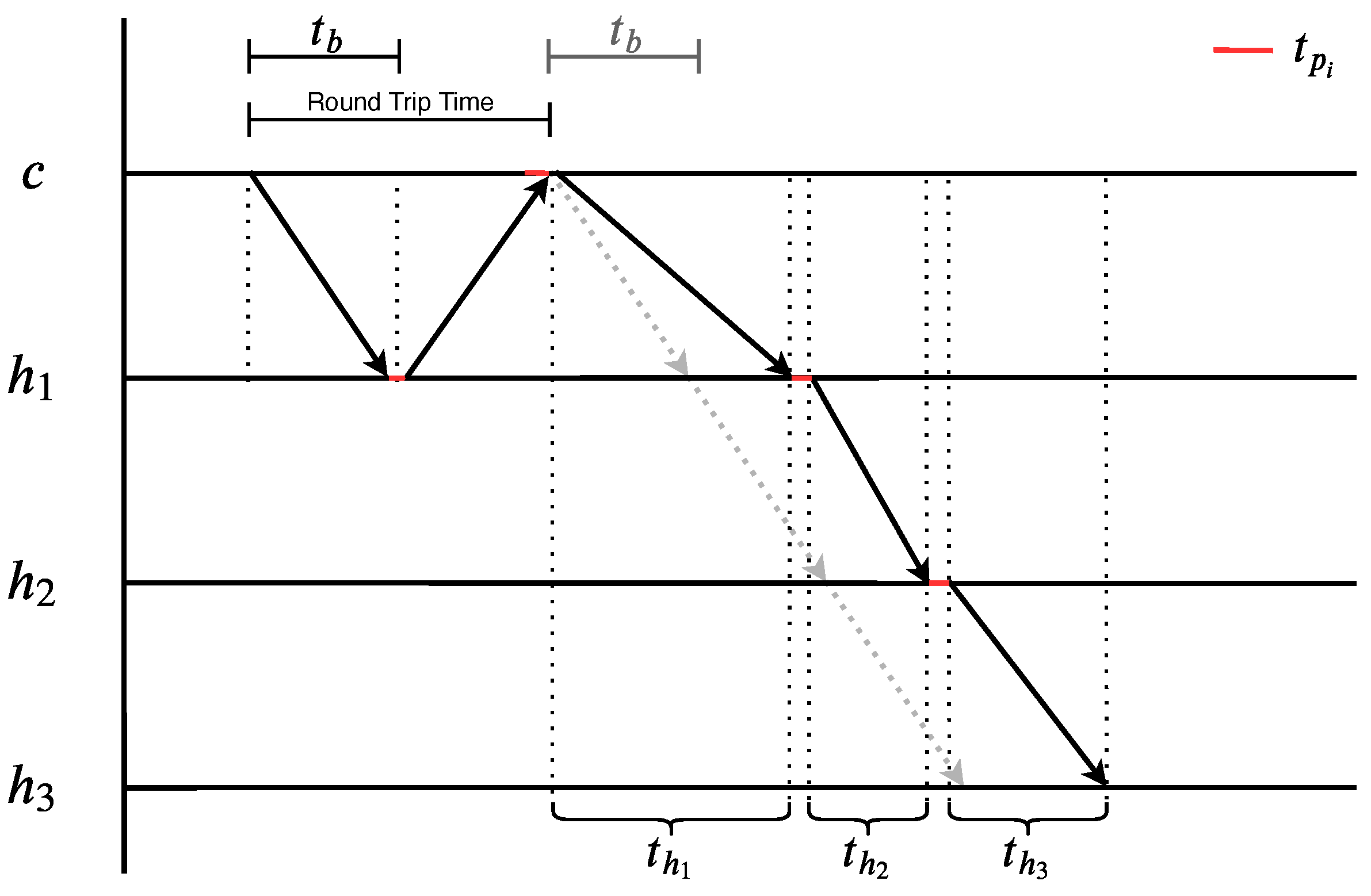
5.2. Remote Synchronization Evaluation on Per-Hop-Basis Time-Stamping

The second experiment aimed to evaluate the synchronization algorithm on a larger scale WSN that operates under real-world conditions. Additionally, a model that predicts the arrival times of each packet on the initiator, which is based on the delay the packet has on each node it reaches, was developed. For evaluation purposes, the experiment was conducted in the Ionian University’s Campus testbed [48] where thick stone walls are the main materials comprising the buildings. A WSN based system was employed which comprises 23 nodes. One (1) of the nodes is the coordinator/initiator and 22 of them operate as routers on the network. In [48] it is mentioned that the WSN topology is highly dependent on current environmental conditions; thus, the topology differs between experiments conducted during variable times of the day. Figure 9 depicts a fully assembled node that is installed in one of the node places inside the testbed’s buildings.

The current experiment used custom-designed code which contains initialization operations that derive all the required network attributes for the proper operation of the algorithms. The attributes are the following: (i) the initiator’s eccentricity, which is used for the synchronization algorithm; (ii) the network topology, useful for the post-processing procedures; and (iii) the tree topology of the network, which was created based on the topology created previously. Each node is assigned with a parent node, hereafter referred to as $p_{r_i}$. The latter creates a routing path for all nodes to transmit any packets back to the initiator from parent to parent. This helps avoid the network overhead of finding the route from a node $r_i$ that wants to transmit a packet to the initiator.

According to the ZigBee protocol when a node transmits a packet, inside its header (i.e., the stored information describing the packet that is about to be transmitted) there can only exist two (2) MAC addresses that correspond to the source and the destination. Before conducting the experiment, all nodes were assigned with a unique node identifier which was a single-byte sized constant. In order for the initiator to be able to recognize the original packet’s source created by a node $r_i$ where $h_{r_i}\ge 2$, the node identifier was inserted to the packet payload.

After the initialization processes, the initiator, denoted by c, synchronizes the WSN according to the algorithm described in Section 4. Each router node $r_i$ that receives the synchronization also calculates the measurement start time, denoted by $m\left(r_i\right)$, based on Equation (4). For the experiment, the measurement packet was set to contain the following information: (i) the measurement timestamp, based on the globally synchronized virtual clock; (ii) the node identifier; (iii) the distance in hops from the initiator; (iv) the hops the synchronization packet traveled before it reached node $r_i$; and (v) the service number from each node the packet goes through. Each time the data packet is transmitted, it is sent to the parent node $p_{r_i}$ as described above. Upon reception, $p_{r_i}$ inserts the global timestamp, which is calculated according to the local clock, and the local service number of the packet. Finally, $p_{r_i}$ retransmits the updated packet to its parent. The above steps are repeated until the packet is received by the c. Note that the synchronization process employs broadcast transmissions while the measurement packets utilize the unicast transmission mechanism.

The entire packet is depicted in Figure 10. Packet type is used for distinguishing between the different packets a node $r_i$ might receive during the experiments. Sync packet contains a counter that shows how many transmissions a synchronization packet is subjected to until it reached the current node. Measure ID is a counter that shows how many measurements $r_i$ has made since the synchronization. Total packets is a counter that shows how many packets a node has serviced so far. This field might contain multiple counters since each node that receives the packet appends its own counter. Service order also gets updated by each node by appending the number of packets it has serviced until the current packet reception. This counter is reset for every new measurement. Next, distance shows the distance of node $r_i$ from c. Node IDs contain multiple node identifications from all the nodes the packet passes through. Finally, timestamps also contain multiple timestamps from every node in the packet’s path to c. Note that information (i.e., total packets, service order, and timestamps) for diagnostics and the synchronization evaluation purposes is introduced in the packet.

The bottom part of Figure 10 depicts a packet example as it is created and communicated from node 5. This packet requires a total of two transmissions in order to reach the initiator, since node 5 does not have a direct link with it (i.e., distance is equal to two). Additionally, each time the packet is transmitted, a timestamp is appended to the packet, the service order (i.e., number of packets that have been processed by the current node where the packet has arrived), and the node ID of the current node. In the example depicted in Figure 10, the packet of data was created from node number 5 and transmitted at time 3,780,459; it first reached node number 2; and it was serviced third in line and transmitted at time 3,780,990. The packet reached the initiator (node number 1) at time 3,781,343. Note that all clocks are synchronized at this point, while all nodes measure time in milliseconds (only for the current packet example).

Two models that attempt to describe the packet arrival times of all nodes to the initiator are assumed. The results from the experimentation procedure are depicted in Figure 11. The blue line depicts the simple model while the green represents the synthetic model that uses more information about each transmitted packet. Finally, the yellow line shows the arrival times recorded by the initiator for each node’s $r_i$ packet.

The simple model follows a scheme where it is considered that each node’s $r_i$ packet arrives at the initiator based on its distance in hops $h_{r_i}$. This is depicted in blue color in Figure 11. This model takes into consideration a small amount of information and the results show that the transmissions cannot take place simultaneously for all nodes that have the same distance from the initiator.

$$si\left(p_i\right)=t_c+t_u\times h_{r_i}.$$

(5)

The synthetic model takes advantage of information related to each transmission that takes place in the network. As already described, the packet of information transmitted by each node—by the time it reaches the initiator—contains information that helps determine a small portion of the delays ($d_{r_n}$) that each one is subjected to while being propagated to the initiator. The current model employs this information to estimate the delivery times of each packet to the initiator. Figure 12 depicts the network’s topology formed during the experiments in the Ionian Campus testbed. For the analysis, this Figure contains only part of the topology, and more specifically the tree topology which uses the predefined paths connecting all nodes to the initiator. Each node is tagged with two numbers $r_i^j$ that contains information related to the results of the experiment depicted in Figure 11, where i represents the Node ID and j shows the order in which the initiator received each packet. For example, node $r_4^8$ is the fourth node in the figure and its packet was the eighth in line that arrived at the initiator. The colors in the current Figure are used to indicate a node’s $r_i$ load of packets. Notice that black is used for the leaves of the tree where those nodes are not parents to any others so they only serve the packets they create. Nodes colored with red outlines serve at least four (4) packets, including their own. The blue outline is used for nodes serving three (3) packets and the green ones only serve two (2).

$$s\left(p_i\right)=t_c+\sum _{n=1}^{n=h_{r_i}}{t}_u\times d_{r_n}.$$

(6)

$p_i$ represents the packet that is being propagated to the initiator from node $r_i$. $d_{r_n}$ represents the delay from the service order in node $r_n$

The result analysis shows that the synthetic model, which uses the delay introduced by the packet congestion on each node $r_i$, has variable results. More specifically, it appears that while the synthetic model curve is lowered, the real arrival times curve tends to move upwards with a smaller rate. Additionally, by comparing the line arrivals of packets to the initiator, it was observed that many nodes such as $r_{10}^6$, despite having bigger distances in hops ($h_{r_{10}}=2$) than $r_3^9$ ($h_{r_3}=1$), managed to transmit it much earlier. This phenomenon is present due to synchronization inaccuracies introduced by the triple broadcast packet transmission employed by the ZigBee protocol during the synchronization phase of the WSN. This phenomenon was described in the previous experiment in Section 5.1. Additionally, another factor that causes variant packet arrival times for the initiator is the CSMA/CA mechanism used for unicast transmissions.

Finally, there are occasions when the initiator did not receive packets from its children at a steady rate. This was caused by the RTS/CTS mechanism employed by the CSMA/CA protocol. A possible scenario that can cause it is when a node $r_2$ ($h_{r_2}=2$) has a packet to transmit to its parent node $r_1$ ($h_{r1}=1$). When this happens, $r_2$ sends an RTS packet which informs all neighboring nodes that $r_2$ has a packet with destination node $r_1$. The latter node then sends back a CTS packet which informs $r_2$ and all nodes that can receive it that $r_1$ is ready to receive the packet. This process causes all nodes that receive either the RTS or CTS packet to postpone their transmissions, resulting in delayed packet reception to the initiator.

6. Discussion

The current section contains a discussion that focuses on an extended version of the results from the experiment described in Section 5.2. The experiment shows that there are very few occasions where the packets from all nodes manage to reach the initiator. It is assumed that this is caused by CSMA/CA retry numbers larger than three (3). Since there are too many antennas competing for transmission in the same channel and the network density is equal to 0.48, there could be many nodes that try sending either their own packets or packets from child nodes more than three times and fail. When a packet transmission occurs from a node, the XBee antenna informs the main Arduino board about the state of the transmission, either successful or failed. The current experiments do not use any mechanism in the main Arduino software for handling the failed transmissions. This is a required future optimization of the system.

The CSMA/CA protocol also creates delays in packet transmissions that cannot be traced by the nodes. This happens when a node has transferred a packet from the main Arduino board to the XBee antenna. The counters used to track the service line of each packet are updated when the received packet has been transferred from the antenna to the mainboard. The current approach for the synthetic model assumed in Section 3 does not take into account these delays since it is indirect information, in the sense that the XBee antennas handle the CSMA/CA operations without informing the mainboard about the state of the procedure, and consequently the nodes are not able to keep track of them.

To assess the effectiveness of the considered approach to provide precise time-correlated SHM, the following case is considered. Supposing that an event, causing vibrations on the structural elements of a building, takes place, it is expected that sensors located close to the initial vibration event should monitor the vibrations earlier than the sensors located at a greater distance. In this case, to be able to use the monitored vibrations to represent the vibration event and its effects on the building, time deviations of the nodes’ clocks should be less than the time needed for the vibrations to propagate between sensors. To consider the proposed approach successful, the resulted values should not surpass a specified deviation limit. To estimate this limit, the following method is utilized.

As described in Section 2 an extensive 2018 work [13] describes the basic principles of wave propagation through the materials of historical buildings. Variant materials induce diverse mechanical properties; thus the propagation of wave-like ambient vibrations varies in terms of the propagation speed through them. For simplicity reasons in the current work, the average propagation speed of transverse waves (which are propagated faster than longitudinal waves) inside the different materials of a historical building is calculated. In [13], different propagation times for the materials comprising the building of their experiments are provided; given these values, the average propagation speed for our case is derived using all speeds provided in the article and is equal to 1.261, 22 m/s, or 1 m/792.88 $\mathsf{\mu }$s.

In the presented SHM system (Section 5.2) the mean distance of all pairs of nodes close-by is about 20 meters. This distance is calculated using the distances of the two different points of the walls where nodes are located using the shortest path connecting them through the structural elements. By using the average propagation speed inside the different materials it is calculated that 1 m can be covered in about $792.88\times {10}^{-6}$ s which is 792.88 $\mathsf{\mu }$s. Thus, it is estimated that the synchronization of the final system with a mean distance of two nodes equal to 20 m, requires that the clock skew be less than 15,8576 ms (20 × 792.88 $\mathsf{\mu }$s) which is the estimated time that the vibrations require in order to be propagated to the structural elements between two sensors. Taking into account the above analysis, it is derived that the synchronization clock skew achieved in the current work can provide an accurate enough time correlation of the WSN collected data, allowing for proper knowledge extraction about the building’s condition.

7. Conclusions and Future Work

Historical buildings are an essential part of all civilizations worldwide and preserving their structural integrity is an important and challenging task. This can be achieved with sensory devices that can monitor environmental conditions. Over the years there have been developed two types of monitoring sensors, active and passive. These systems originally consisted of sensory devices interconnected using a cabling infrastructure. The technological advances of the last few decades enabled them to become wireless systems which provide them with more liberty of deployment and also lower cost requirements.

In the current work, a low-cost WSN-based system and a synchronization algorithm calibrated for use in historical buildings are developed. The algorithm employs topological information regarding the WSN in order to accurately synchronize all nodes using a multi-hop scheme. The experiments conducted aim to evaluate the synchronization algorithm on both laboratory conditions and real-world scenarios on historical buildings. The results show that under laboratory conditions a WSN comprising four nodes can synchronize with a mean clock skew of about 2000 $\mathsf{\mu }\mathrm{s}$.

The second experiment uses an extended WSN that operates on the Ionian University’s campus testbed where it is shown that the synchronization of all nodes on the assumed system is highly dependent on the CSMA/CA protocol employed by ZigBee. The results show that each node’s synchronization is affected by the variations in the packet transmissions created from different collision avoidance and broadcast schemes.

The conducted experiments depict that the synchronization algorithm and the WSN developed for the current study provide sufficient time synchronization for the proper correlation of ambient vibrations from multiple independent nodes. However, since the XBee antennas that handle the wireless communication between nodes use the CSMA/CA protocol, this poses a limitation. In the case where multiple nodes need to transmit measurements due to a sudden event (e.g., earthquake), there might be many data packets that do not get transferred due to network congestion (i.e., a large number of nodes is trying to use the communication medium, the air, at the same time, resulting in unsuccessful transmissions).

The current implementation does not provide the WSN with any scheme that handles lost transmissions which is a potential future topic to study. It is worth pointing out that if a scheme is employed for lost packet handling, the WSN might not be able to provide real-time information since the packet handling will require additional time.

Additionally, as future work, the synchronization algorithm can be further improved by employing more complex networking techniques. In the current approach, when a node receives a synchronization packet, it retransmits it only if it is the first synchronization packet received. Every time a node transmits the packet, an additional random delay is added which cannot be captured and calculated to achieve a smaller time difference between the WSN’s nodes. A possible solution to this issue is to select a subset of nodes that transmit the synchronization packet. These nodes need to be able to communicate with at least one of the nodes in the subset, and at least one of them is required to have a direct connection to the initiator (i.e., the node that starts the synchronization). Additionally, the nodes that are not included in the subset need to have at least one direct connection to the subset to receive a synchronization packet.

Taking into account that the system can collect accurate time-correlated measurements of ambient vibrations, a visualization system can be developed. This system can include a 3-dimensional representation of a structure with the nodes of the WSN embedded into the equivalent places inside the virtual environment. The system could provide the visualization application either with collected measurements in real-time or with stored measurements upon request to provide a comprehensible and user-friendly representation of the detected events. The fact that the collected measurements are accurately time-correlated enables that such visualization simulations would provide meaningful representations of a vibration event where the propagation of the vibrations in the structural elements could be visualized effectively and even simulate the potential impact on the structure.

References

1. Farrar, C.R.; Worden, K. An introduction to structural health monitoring. Philos. Trans. R. Soc. A Math. Phys. Eng. Sci. 2006, 365, 303–315. [Google Scholar] [CrossRef]
2. Janapati, V.; Kopsaftopoulos, F.; Li, F.; Lee, S.J.; Chang, F.K. Damage detection sensitivity characterization of acousto-ultrasound-based structural health monitoring techniques. Struct. Health Monit. 2016, 15, 143–161. [Google Scholar] [CrossRef]
3. Deivasigamani, A.; Daliri, A.; Wang, C.; John, S. A review of passive wireless sensors for structural health monitoring. Mod. Appl. Sci. 2013, 7, 57–76. [Google Scholar] [CrossRef]
4. Jo, H.; Rice, J.A.; Spencer, B.F., Jr.; Nagayama, T. Development of high-sensitivity accelerometer board for structural health monitoring. In Sensors and Smart Structures Technologies for Civil, Mechanical, and Aerospace Systems 2010; International Society for Optics and Photonics: San Diego, CA, USA, 2010; Volume 7647, p. 764706. [Google Scholar]
5. Rashid, R.A.; Ahmad, A.G. Overview of maintenance approaches of historical buildings in Kuala Lumpur–a current practice. Procedia Eng. 2011, 20, 425–434. [Google Scholar] [CrossRef] [Green Version]
6. Celebi, M. Seismic Instrumentation of Buildings (with Emphasis on Federal Buildings); Technical Report; Citeseer: Menlo Park, CA, USA, 2002. [Google Scholar]
7. Ishikawa, K.I.; Mita, A. Time synchronization of a wired sensor network for structural health monitoring. Smart Mater. Struct. 2007, 17, 015016. [Google Scholar] [CrossRef] [Green Version]
8. Akyildiz, I.; Su, W.; Sankarasubramaniam, Y.; Cayirci, E. Wireless sensor networks: A survey. Comput. Netw. 2002, 38, 393–422. [Google Scholar] [CrossRef] [Green Version]
9. Oikonomou, K.; Koufoudakis, G.; Kavvadia, E.; Chrissikopoulos, V. A wireless sensor network innovative architecture for ambient vibrations structural monitoring. In Key Engineering Materials; Trans Tech Publ.: Zurich, Switzerland, 2015; Volume 628, pp. 218–224. [Google Scholar]
10. Seah, W.K.; Eu, Z.A.; Tan, H.P. Wireless sensor networks powered by ambient energy harvesting (WSN-HEAP)-Survey and challenges. In Proceedings of the IEEE 2009 1st International Conference on Wireless Communication, Vehicular Technology, Information Theory and Aerospace & Electronic Systems Technology, Aalborg, Denmark, 17–20 May 2009; pp. 1–5. [Google Scholar]
11. Shaikh, F.K.; Zeadally, S. Energy harvesting in wireless sensor networks: A comprehensive review. Renew. Sustain. Energy Rev. 2016, 55, 1041–1054. [Google Scholar] [CrossRef]
12. Tokognon, C.A.; Gao, B.; Tian, G.Y.; Yan, Y. Structural health monitoring framework based on Internet of Things: A survey. IEEE Internet Things J. 2017, 4, 619–635. [Google Scholar] [CrossRef]
13. Orenday-Tapia, E.E.; Pacheco-Martínez, J.; Padilla-Ceniceros, R.; López-Doncel, R.A. In situ and nondestructive characterization of mechanical properties of heritage stone masonry. Environ. Earth Sci. 2018, 77, 286. [Google Scholar] [CrossRef]
14. Bezas, K.; Komianos, V.; Oikonomou, K.; Koufoudakis, G.; Tsoumanis, G. Structural Health Monitoring in Historical Buildings Using A Low Cost Wireless Sensor Network. In Proceedings of the 2019 South Eastern European Design Automation, Computer Engineering, Computer Networks and Social Media Conference (SEEDA-CECNSM), Piraeus, Greece, 20–22 September 2019. [Google Scholar]
15. De Stefano, A.; Matta, E.; Clemente, P. Structural health monitoring of historical heritage in Italy: Some relevant experiences. J. Civ. Struct. Health Monit. 2016, 6, 83–106. [Google Scholar] [CrossRef]
16. De Stefano, A.; Clemente, P. SHM on historical heritage. Robust methods to face large uncertainties. In Proceedings of the 1st International Conference on Structural Condition Assessment, Monitoring and Improvement, Perth, Australia, 12–14 December 2005; pp. 12–14. [Google Scholar]
17. Boscato, G.; Dal Cin, A.; Russo, S.; Sciarretta, F. SHM of historic damaged churches. In Advanced Materials Research; Trans Tech Publ.: Zurich, Switzerland, 2014; Volume 838, pp. 2071–2078. [Google Scholar]
18. Gattulli, V.; Lepidi, M.; Potenza, F. Dynamic testing and health monitoring of historic and modern civil structures in Italy. Struct. Monit. Maint. 2016, 3, 71. [Google Scholar] [CrossRef]
19. Pierdicca, A.; Clementi, F.; Isidori, D.; Concettoni, E.; Cristalli, C.; Lenci, S. Numerical model upgrading of a historical masonry palace monitored with a wireless sensor network. Int. J. Mason. Res. Innov. 2016, 1, 74–98. [Google Scholar] [CrossRef]
20. Noel, A.B.; Abdaoui, A.; Elfouly, T.; Ahmed, M.H.; Badawy, A.; Shehata, M.S. Structural health monitoring using wireless sensor networks: A comprehensive survey. IEEE Commun. Surv. Tutor. 2017, 19, 1403–1423. [Google Scholar] [CrossRef]
21. Riggio, M.; Dilmaghani, M. Structural health monitoring of timber buildings: A literature survey. Build. Res. Inf. 2019, 1–21. [Google Scholar] [CrossRef]
22. Sadler, B.M.; Swami, A. Synchronization in sensor networks: An overview. In Proceedings of the MILCOM 2006–2006 IEEE Military Communications Conference, Washington, DC, USA, 23–25 October 2006; pp. 1–6. [Google Scholar]
23. Lasassmeh, S.M.; Conrad, J.M. Time synchronization in wireless sensor networks: A survey. In Proceedings of the IEEE SoutheastCon 2010 (SoutheastCon), Concord, NC, USA, 18–21 March 2010; pp. 242–245. [Google Scholar] [CrossRef]
24. Swain, A.R.; Hansdah, R. A model for the classification and survey of clock synchronization protocols in WSNs. Ad Hoc Netw. 2015, 27, 219–241. [Google Scholar] [CrossRef]
25. Elson, J.; Girod, L.; Estrin, D. Fine-grained network time synchronization using reference broadcasts. ACM SIGOPS Oper. Syst. Rev. 2002, 36, 147–163. [Google Scholar] [CrossRef]
26. Noh, K.; Serpedin, E.; Qaraqe, K. A New Approach for Time Synchronization in Wireless Sensor Networks: Pairwise Broadcast Synchronization. IEEE Trans. Wirel. Commun. 2008, 7, 3318–3322. [Google Scholar] [CrossRef]
27. Kim, S.; Pakzad, S.; Culler, D.; Demmel, J.; Fenves, G.; Glaser, S.; Turon, M. Health monitoring of civil infrastructures using wireless sensor networks. In Proceedings of the 6th International Conference on Information Processing in Sensor Networks, Cambridge, MA, USA, 25–27 April 2007; pp. 254–263. [Google Scholar]
28. Maróti, M.; Kusy, B.; Simon, G.; Lédeczi, Á. The flooding time synchronization protocol. In Proceedings of the 2nd International Conference on Embedded Networked Sensor Systems, Baltimore, MD, USA, 3–5 November 2004; pp. 39–49. [Google Scholar]
29. Mock, M.; Frings, R.; Nett, E.; Trikaliotis, S. Continuous clock synchronization in wireless real-time applications. In Proceedings of the 19th IEEE Symposium on Reliable Distributed Systems SRDS-2000, Nurnberg, Germany, 16–18 October 2000; pp. 125–132. [Google Scholar]
30. Shi, F.; Tuo, X.; Yang, S.; Li, H.; Shi, R. Multiple two-way time message exchange (ttme) time synchronization for bridge monitoring wireless sensor networks. Sensors 2017, 17, 1027. [Google Scholar] [CrossRef] [Green Version]
31. Xu, N.; Rangwala, S.; Chintalapudi, K.K.; Ganesan, D.; Broad, A.; Govindan, R.; Estrin, D. A wireless sensor network for structural monitoring. In Proceedings of the 2nd International Conference on Embedded Networked Sensor Systems, Baltimore, MD, USA, 3–5 November 2004; pp. 13–24. [Google Scholar]
32. Wang, Y.; Lynch, J.P.; Law, K.H. A wireless structural health monitoring system with multithreaded sensing devices: Design and validation. Struct. Infrastruct. Eng. 2007, 3, 103–120. [Google Scholar] [CrossRef] [Green Version]
33. Shannon, J.; Melvin, H.; Ruzzelli, A.G. Dynamic flooding time synchronisation protocol for WSNs. In Proceedings of the 2012 IEEE Global Communications Conference (GLOBECOM), Anaheim, CA, USA, 3–7 December 2012; pp. 365–371. [Google Scholar]
34. Su, W.; Akyildiz, I.F. Time-diffusion synchronization protocol for wireless sensor networks. IEEE/ACM Trans. Netw. (TON) 2005, 13, 384–397. [Google Scholar] [CrossRef]
35. Ganeriwal, S.; Kumar, R.; Srivastava, M.B. Timing-sync protocol for sensor networks. In Proceedings of the 1st International Conference on Embedded Networked Sensor Systems, Los Angeles, CA, USA, 5–7 November 2003; pp. 138–149. [Google Scholar]
36. Sommer, P.; Wattenhofer, R. Gradient clock synchronization in wireless sensor networks. In Proceedings of the 2009 International Conference on Information Processing in Sensor Networks. IEEE Computer Society, San Francisco, CA, USA, 13–16 April 2009; pp. 37–48. [Google Scholar]
37. Li, Q.; Rus, D. Global clock synchronization in sensor networks. IEEE Trans. Comput. 2006, 55, 214–226. [Google Scholar]
38. PalChaudhuri, S.; Saha, A.K.; Johnson, D.B. Adaptive Clock Synchronization in Sensor Networks. In Proceedings of the 3rd International Symposium on Information Processing in Sensor Networks, Berkeley, CA, USA, 27 April 2004; IPSN ’04. ACM: New York, NY, USA, 2004; pp. 340–348. [Google Scholar] [CrossRef] [Green Version]
39. Phanish, D.; Garver, P.; Matalkah, G.; Landes, T.; Shen, F.; Dumond, J.; Abler, R.; Zhu, D.; Dong, X.; Wang, Y.; et al. A wireless sensor network for monitoring the structural health of a football stadium. In Proceedings of the 2015 IEEE 2nd World Forum on Internet of Things (WF-IoT), Milan, Italy, 14–16 December 2015; pp. 471–477. [Google Scholar]
40. Chen, Z.; Li, D.; Huang, Y.; Tang, C. Event-triggered communication for time synchronization in WSNs. Neurocomputing 2016, 177, 416–426. [Google Scholar] [CrossRef]
41. Fanarioti, S.; Tsipis, A.; Giannakis, K.; Koufoudakis, G.; Christopoulou, E.; Oikonomou, K.; Stavrakakis, I. A Proposed Algorithm for Data Measurements Synchronization in Wireless Sensor Networks. In Proceedings of the Second International Balkan Conference on Communications and Networking 2018 (BalkanCom’18), Podgorica, Montenegro, 6–8 June 2018; pp. 1–5. [Google Scholar]
42. Casarin, F.; Modena, C.; Aoki, T.; da Porto, F.; Lorenzoni, F. Structural Health Monitoring of historical buildings: Preventive and post-earthquake controls. In Proceedings of the 5th International Conference on Structural Health Monitoring of Intelligent Infrastructure (SHMII-5), Cancun, Mexico, 11–15 December 2011; pp. 11–15. [Google Scholar]
43. Arduino. Arduino Mega 2560 Rev3. Available online: https://store.arduino.cc/mega-2560-r3 (accessed on 17 March 2020).
44. Arduino. Arduino Wireless SD Shield. Available online: https://store.arduino.cc/arduino-wirelss-sd-shield (accessed on 17 March 2020).
45. Digi. XBee-PRO Zigbee Through-Hole (Wire Antenna). Available online: https://www.digi.com/products/models/xbp24cz7wit-004 (accessed on 17 March 2020).
46. Andrewrapp. andrewrapp/xbee-arduino. Available online: https://github.com/andrewrapp/xbee-arduino (accessed on 17 March 2020).
47. InvenSense. MPU-6050 Six-Axis (Gyro + Accelerometer) MEMS MotionTracking™ Devices. Available online: https://www.invensense.com/products/motion-tracking/6-axis/mpu-6050/ (accessed on 17 March 2020).
48. Alvanou, A.G.; Zervopoulos, A.; Papamichail, A.; Bezas, K.; Vergis, S.; Stylidou, A.; Tsipis, A.; Komianos, V.; Tsoumanis, G.; Koufoudakis, G.; et al. CaBIUs: Description of the Enhanced Wireless Campus Testbed of the Ionian University. Electronics 2020, 9, 454. [Google Scholar] [CrossRef] [Green Version]
Figure 1. A WSN node assembled including all four components. The sensor connected on the white breadboard is the accelerometer that senses the ambient vibrations of the structure.
Heritage 03 00044 g001
Figure 2. Packet structure (the top part of the figure) for information communication in the considered implementation as they are being transmitted by each router node. The bottom part depicts a packet example similar to the ones communicated by the WSN nodes.
Heritage 03 00044 g002
Figure 3. The WSN before and after the synchronization. The WSN synchronization phase is depicted within the two vertical dashed lines.
Heritage 03 00044 g003
Figure 4. The two phases of the synchronization algorithm along with the guard period denoted as g. The vertical dashed line at the end of the guard period is the time of the first measurement calculated by all nodes of the network based on their distances from the initiator.
Heritage 03 00044 g004
Figure 5. The code execution interrupt events’ experimental WSN topology. The initiator has only one neighbor and its eccentricity equals two.
Heritage 03 00044 g005
Figure 6. Synchronization cycles from all nodes combined.
Heritage 03 00044 g006
Figure 7. The figures contain the local time differences (Δt) from the initiator’s synchronization clock ( t c ) organized in histograms. (a) Time difference in all synchronization cycles on node r 2 synchronization cycles where h r 2 (b) Time difference in all synchronization cycles of node r 3 synchronization cycles where h r 3 (c) Time difference in all synchronization cycles of node r 1 synchronization cycles where h r 1 .
Heritage 03 00044 g007
Figure 8. This figure depicts the real-world operation of the synchronization process that changes depending on the CSMA/CA operation. t p i represents the processing time of each node i. This delay is variable and depends on the load the node has upon the packet reception.
Heritage 03 00044 g008
Figure 9. A fully assembled node installed in one of the buildings where the experiments were conducted. The red rectangle depicts the accelerometer; the battery that powers all the components is inside the green rectangle. The main Arduino board where the XBee antenna and the wireless shield are contained is within the blue rectangle.
Heritage 03 00044 g009
Figure 10. Packet structure used during the second experiment for information communication and synchronization evaluation. The bottom part depicts an example packet.
Heritage 03 00044 g010
Figure 11. The simple (marked in blue color) and the synthetic (marked in green color) models for packet time arrivals on the initiator. Additionally contained is the arrival time measured by the initiator (marked in yellow color).
Heritage 03 00044 g011
Figure 12. The WSN topology set up during the experiment. The figure depicts the tree topology of the network that is used for propagating the data packets to the sink node (i.e., initiator, c).
Heritage 03 00044 g012