Nonlinear Metamaterial Lenses for Inductive Power Transmission Systems Using Duffing-Resonator Based Unit Cells

Abstract

Metamaterials (MTMs) based on a periodic array of resonant coils have been shown to behave as μ-negative (MNG), enabling the focusing of magnetic flux. The phenomenon has been deployed by designers to boost the efficiency of many inductively coupled systems, such as magnetic resonance imaging, underwater and underground communications, and charging base stations (CBS) for consumer electronics and implanted devices. However, due to their dependency on high-Q unit cells, linear MNG-like MTMs have limited bandwidth, restricting their use in many applications, notably in near-field simultaneous wireless information and power transmission (NF-SWIPT) systems. To improve the tight constraints of the amplitude-bandwidth trade-off of artificial magnetic lenses, this paper presents a theoretical analysis of nonlinear MTMs based on a lattice of Duffing resonators (DRs). Additionally, it introduces a criterium for the quantification and evaluation of the amplitude-bandwidth enhancement. The analytical results are based on a circuit model and further verified by numerical simulations using commercial software. The preliminary findings in this paper open up possibilities for nonlinear MTM lenses and can be applied to enhance the linear amplitude-bandwidth limit.

1. Introduction

Over the last 20 years or so, flat, compact, and light artificial lenses inspired by metamaterials (MTMs) have attracted a lot of attention due to their flexibility, controllability, low profile, and reduced cost. If the periodicity of such arrays and the dimensions of their cells are much smaller than their operating wavelength, they can be shown to behave as ideal left-handed materials with negative constitutive parameters, such as magnetic permeability $\mu$, electric permittivity $\epsilon$, and/or refraction index $n$, around its resonance frequency. As extensively discussed in [1,2,3], the sign-changing inside the MTM (for 3D structures) or at its surface (for 2D structures) causes an apparent gain of the incident electromagnetic (EM) modes caused by the sign inversion of the propagation constant $\beta$. By inverting the phase gain of the EM fields, the MTM slab causes a focalization effect like conventional “positive” lenses. The advantage of such a strategy is that such “negative” lenses do not require a 3D nonuniform distribution of its constitutive parameters in order to focus the EM fields as the “positive” ones do. This means that the concave or convex geometry of conventional lenses can be simplified to a flat structure, reducing the system’s profile and its manufacturing costs. Another advantage of MTM-based lenses is that their spatial and frequency responses can be easily reconfigured by controlling the current and voltage distribution of their unit cells.

In the context of inductive-coupling-based systems, MTMs consisting of a periodic array of resonant coils are of great interest because of their ability to synthesize and create $\mu$-negative (MNG) material like response [4]. For example, inductive power transmission (IPT) systems can take advantage of MNG-like MTMs to focus the magnetic flux and reduce the system’s power transfer efficiency (PTE) decay with the operating distance. The main properties and focalization effect of MTMs based on linear resonators have been extensively discussed in [5,6]. As has been discussed in [7], the MNG MTM slab at its operating frequency supports the propagation of magneto-inductive (MI) waves on its surface capable of coupling with the evanescent magnetic modes generated by the transmitter (TX) driver, which generates the apparent focusing process perceived as band-limited amplification, gain, or enhanced coupling. Since MI wave propagation on the MTMs’ surface is a collective behavior, it is much more tolerant to fabrication defects or misalignments. As discussed in [8], MTM-assisted IPT systems are highly tolerant to misalignments between the TX and receiver (RX) drivers due to the possibility of the excitement of multiple spatial modes of the magnetic flux ${\varphi }_m$. Other investigations have also shown that the deployment of hybrid unit cells with negative and near-zero magnetic permeability could ameliorate the MTM gain [9].

However, in all the previously mentioned works, the amazing properties of these MTMs are limited to extremely narrow bands because of the high-Q cells required to obtain an MNG-like response. Although MTMs have been successfully employed in many IPT applications [10], including biomedical ones [11], the high frequency selectiveness of these artificial lenses limits their potential use on near-field simultaneous wireless information and power transmission (NF-SWPIT) systems. Considering that NF-SWIPTs are the most reliable and environmentally friendly systems in many future 5G and 6G applications, such as underwater and underground communications, wearable and implanted wireless sensor networks, and charging base stations (CBS) for electronics and electric vehicles, the development of MTM lenses with enhanced bandwidth characteristics are of great interest.

Since linear resonators’ amplitude bandwidth is tightly limited by the circuit’s Q-factor, nonlinear resonators, such as the Duffing resonator (DR), must be considered in order to extend the operating bandwidth of the MTM’s MNG response. DRs are dynamical systems with chaotic behavior, which have been largely employed in the past as chaos-based secure communication and random number generation [12]. Only recently mechanical and electrical engineers have started to exploit the multistability characteristics of DRs to improve the amplitude-bandwidth trade-off in high-Q systems [13,14,15]. One of the advantages of DRs in relationship to other nonlinear unit cells proposed in the literature, such as in [16], is that they do not require any active control to overcome the linear amplitude-bandwidth limit.

This work theoretically investigates the potential use of nonlinear Duffing resonators (DRs) as the unit cells of MNG lenses with enhanced amplitude-bandwidth characteristics. Such a nonlinear resonance has been applied to radiofrequency (RF) energy harvesters and wireless power transmission using strongly coupled coils [14,15]. Varactors on metamaterial cells have been proposed for dynamic tunability [17]. To the authors’ best knowledge, no one has ever investigated the possibility of applying DRs as the unit cell of nonlinear MTM-based MNG lenses for NF-SWPIT with improved amplitude-bandwidth performance. Besides that, this paper presents, for the first time, a criterium to quantify the amplitude-bandwidth enhancement due to the DR nonlinear response. The presented analytical results are supported by numerical simulations using Keysight Pathwave ADS 2021.

2. Materials and Methods

2.1. General Circuit Analysis Solution of MTM-Assisted IPT Systems

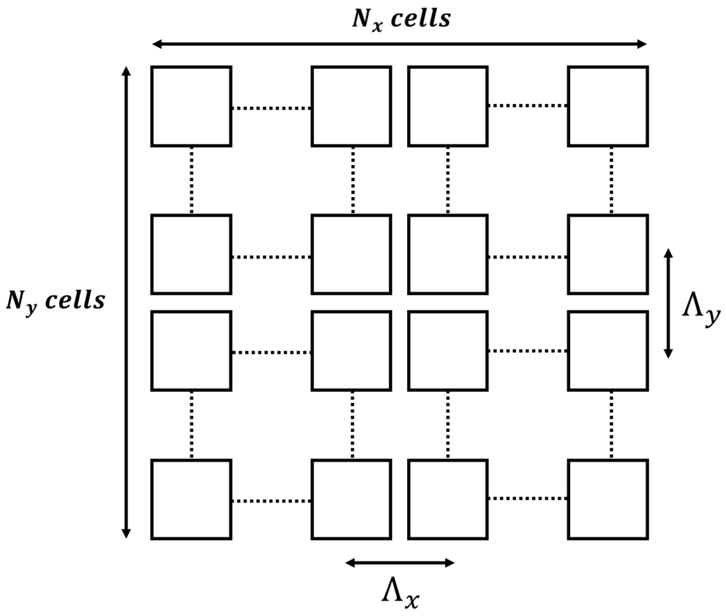
Assuming that the MTM is formed by a square lattice with $N_x=N_y=N$ with constant periodicity ${\mathsf{\Lambda }}_{\mathrm{x}}={\mathsf{\Lambda }}_{\mathrm{y}}=\mathsf{\Lambda }$ (see Figure 1), the circuit analysis of the proposed system results in a $N$ by $N$ problem, whose elements are given by:

$$Z_{cell}{I}_n+j\omega {\displaystyle \sum }_{\begin{array}{c}m=1\\ m\ne n\end{array}}^{N^2}{M}_{nm}{I}_m=-j\omega \left(M_{n,TX}{I}_{TX}+M_{n,RX}{I}_{RX}\right), n=\left[1,N^2\right]$$

(1)

where $Z_{cell}$ is the equivalent impedance of the MTM unit cell, $M_{nm}$ is the mutual inductance between the cell $n$ and $m$ of the MTM slab, $M_{n,TX}$ is the mutual inductance between cell $n$ and the TX coil, $M_{n,RX}$ is the mutual inductance between cell $n$ and the RX coil, $I_n$ and $I_m$ are the currents in the $n$ and $m$ cells, respectively, and $\omega$ is the angular frequency.

Making the simplifying hypothesis that the current in the RX coil is negligible in comparison to the current in the TX coil ($I_{RX}\ll I_{TX}$), the problem can be rewritten in the matrix form as follows:

$$\stackrel{=}{Z}\overline{I}={\overline{V}}_s$$

(2a)

$$\stackrel{=}{Z}=\left[\begin{array}{ccccc}{Z}_{cell}& j\omega M_{1,2}& \dots & j\omega M_{1,N-1}& j\omega M_{1,N}\\ j\omega M_{2,1}& Z_{cell}& \dots & j\omega M_{2,N-1}& j\omega M_{2,N}\\ ⋮& ⋮& \ddots & ⋮& ⋮\\ j\omega M_{N-1,1}& j\omega M_{N-1,2}& \dots & Z_{cell}& j\omega M_{N-1,N}\\ j\omega M_{N,1}& j\omega M_{N,2}& \cdots & j\omega M_{N,N-1}& Z_{cell}\end{array}\right]$$

(2b)

$$\overline{I}=\left[\begin{array}{c}{I}_1\\ I_2\\ ⋮\\ I_{N^2-1}\\ I_{N^2}\end{array}\right]$$

(2c)

$$\overline{V_s}=\left[\begin{array}{c}-j\omega M_{1,TX}{I}_{TX}\\ -j\omega M_{1,TX}{I}_{TX}\\ ⋮\\ -j\omega M_{N^2-1,TX}{I}_{TX}\\ -j\omega M_{N^2,TX}{I}_{TX}\end{array}\right]$$

(2d)

If all the $M_{nm}$ and $M_{n,TX}$ coefficients are known by analytical or numerical computing, the solution of the system is then given by:

$$\overline{I}={\stackrel{=}{Z}}^{-1}\overline{V_s}$$

(3)

As expressed in (2) and (3), each individual MTM cell current $I_n$ is affected not only by the TX coil excitation but also by the current in all other cells due to their mutual coupling. This effect is particularly strong and dominated by the mutual coupling between adjacent cells. Because of that, the resonance frequency ${\omega }_0$ of the unit cell and the MTM operating frequency ${\omega }_{MTM}$ (the maximum gain frequency) are slightly different and obey the following relationship based on the sign of the magnetic coupling ${\kappa }_m$:

$$\begin{array}{c}{\omega }_0>{\omega }_{MTM} if {\kappa }_m>0\\ {\omega }_0<{\omega }_{MTM} if {\kappa }_m<0\end{array}$$

(4)

where ${\kappa }_m>0$ represents a coaxial and ${\kappa }_m<0$ represents a coplanar coupling among the cells. For practical reasons, the coplanar coupling between the cells is the most common scenario.

If the vector $\overline{I}$ can be obtained from (3), then MTM power gain at the receiver plane is given by:

$$G_{MTM}\triangleq {\left(\frac{S_{21,MTM}}{S_{21,0}}\right)}^2={\left(1+{\displaystyle \sum }_{n=1}^{N^2}\frac{M_{n,RX}{I}_n}{M_{RX,TX}{I}_{TX}}\right)}^2$$

(5)

where $S_{21,0}$ and $S_{21,MTM}$ are the system’s transmission coefficient without and with an MTM inside the inductive link, respectively, and $M_{RX,TX}$ is the mutual inductance between the TX and the RX. Notice from (5) that $G_{MTM}$ basically comes from the energy stored in the MTM cells transmitted to the RX coil by $M_{n,RX}$.

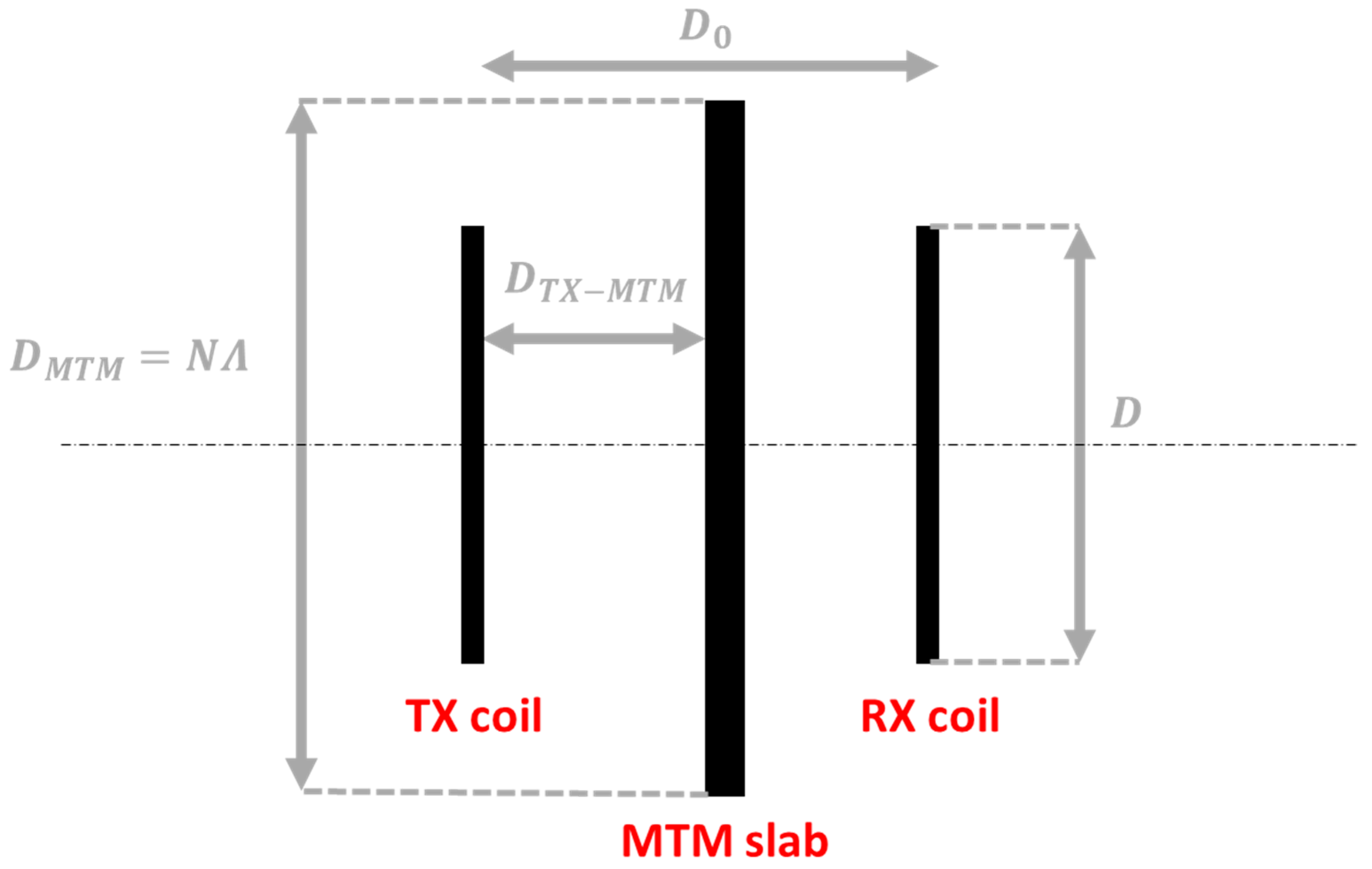
Although it is not possible to solve (3) when $Z_{cell}$ is nonlinear, the analytical investigation of the linear case can be useful to understand the basic mechanism of the MTM near-field focalization.

For example, let us consider an IPT system consisting of two coupled coils with one MTM lens, as shown in Figure 2. The unit cell circuit is assumed to be a planar coil connected in series with a linear capacitance. For the considered numerical example, it is assumed a square lattice with $N=4$, $\mathsf{\Lambda }=2.3 \mathrm{cm}$, $D=10 \mathrm{cm}$, $D_0=6 \mathrm{cm}$, $D_{TX-MTM}=3 \mathrm{cm}$, ${\omega }_0=1$, $L_{cell}=1$, $C_{cell}=0.1$, and $I_s=1$.

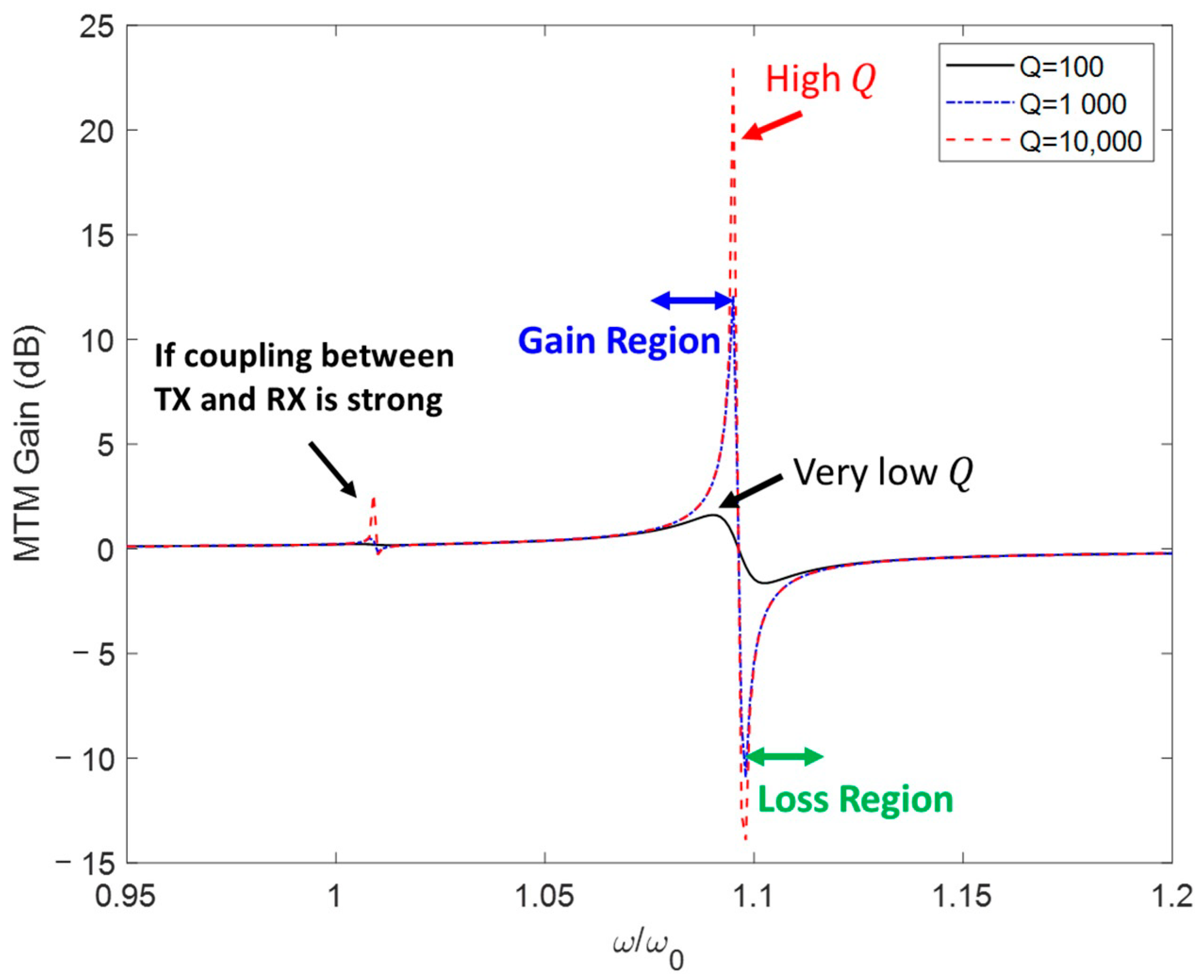
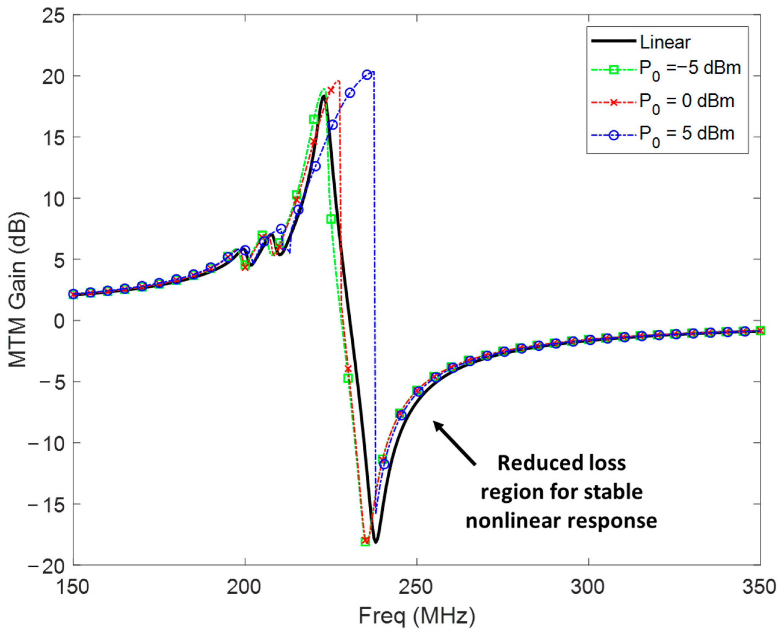
Applying the formalism described in (1)–(5), the presence of the MTM into the inductive link causes a non-negligible $G_{MTM}$ to be obtained in a narrowband region close to the unit-cell resonance ${\omega }_0$, as shown in Figure 3. As expected, ${\omega }_{MTM}$ is slightly higher than ${\omega }_0$ since the coupling between the MTM cells is coplanar (${\kappa }_m<0$). 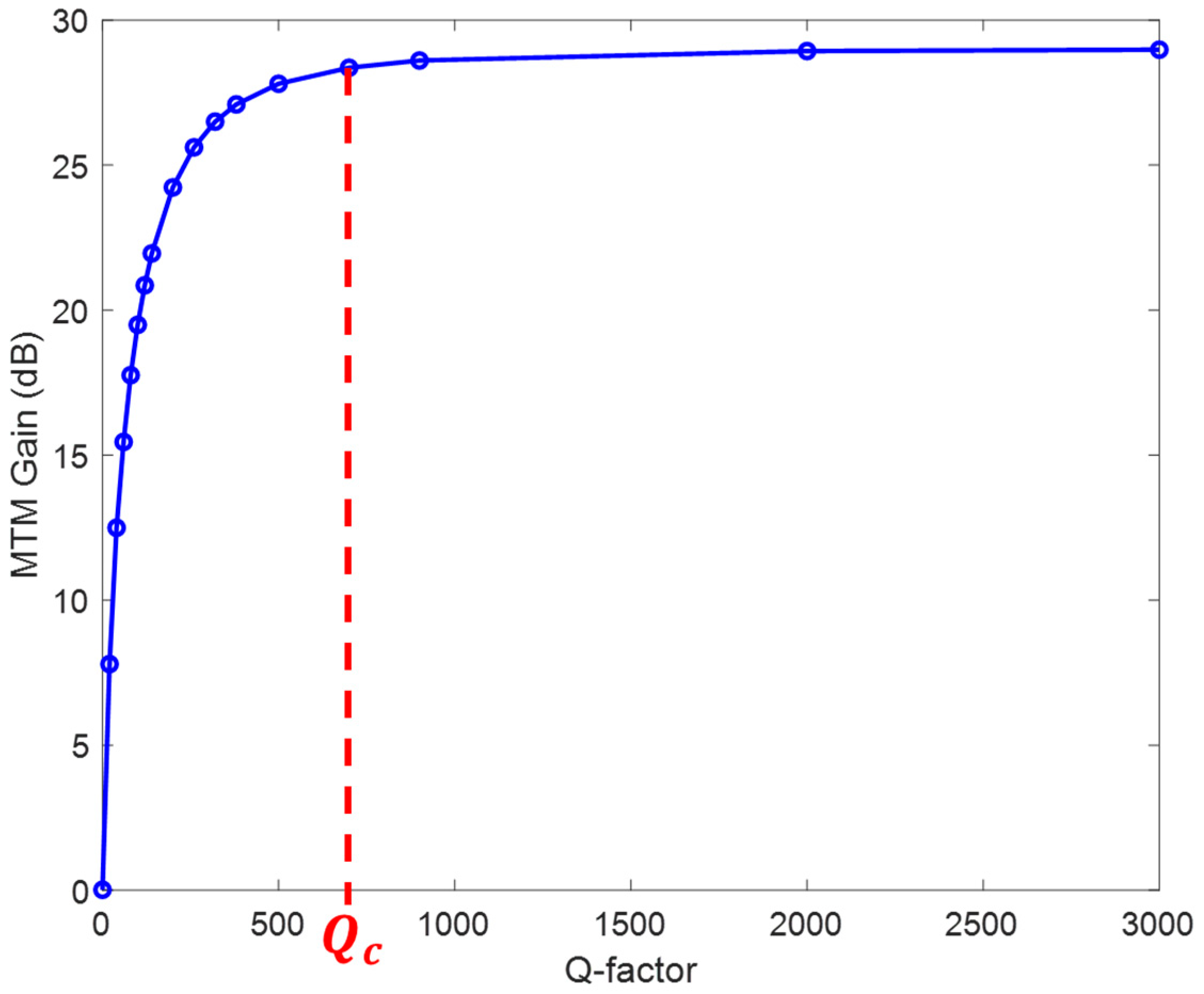However, if TX and RX coils are in close $D_0<D$, a secondary, low gain region can be perceived around ${\omega }_0$ due to the strong coupling between the drivers. Due to the anti-resonance phenomenon that exists between two coupled coils, the gain region induced by the MTM is immediately followed by a loss region. The existence of a loss region in linear MTM-assisted IPT systems makes them quite sensible to frequency shifts. Out of these two special regions around the resonance and anti-resonance, the MTM is completely transparent to the system (null gain). As shown in Figure 4, MTM gain at ${\omega }_{MTM}$ is basically a function of the Q-factor of the cells until this effect saturates above a critical $Q_c$. Essentially, $Q_c$ marks the maximum magnetic energy that can be stored by the cell.

Notice that, according to (5), MTM gain is proportional to $M_{n,RX}$ and inversely proportional to $M_{RX,TX}$. So, despite $Q$, an attenuation of the maximum MTM gain is expected if TX and RX coils are very strongly coupled and if the coupling between the unit cells and the TX coil is too weak.

2.2. Linear Series-Connected Unit-Cell Parameters

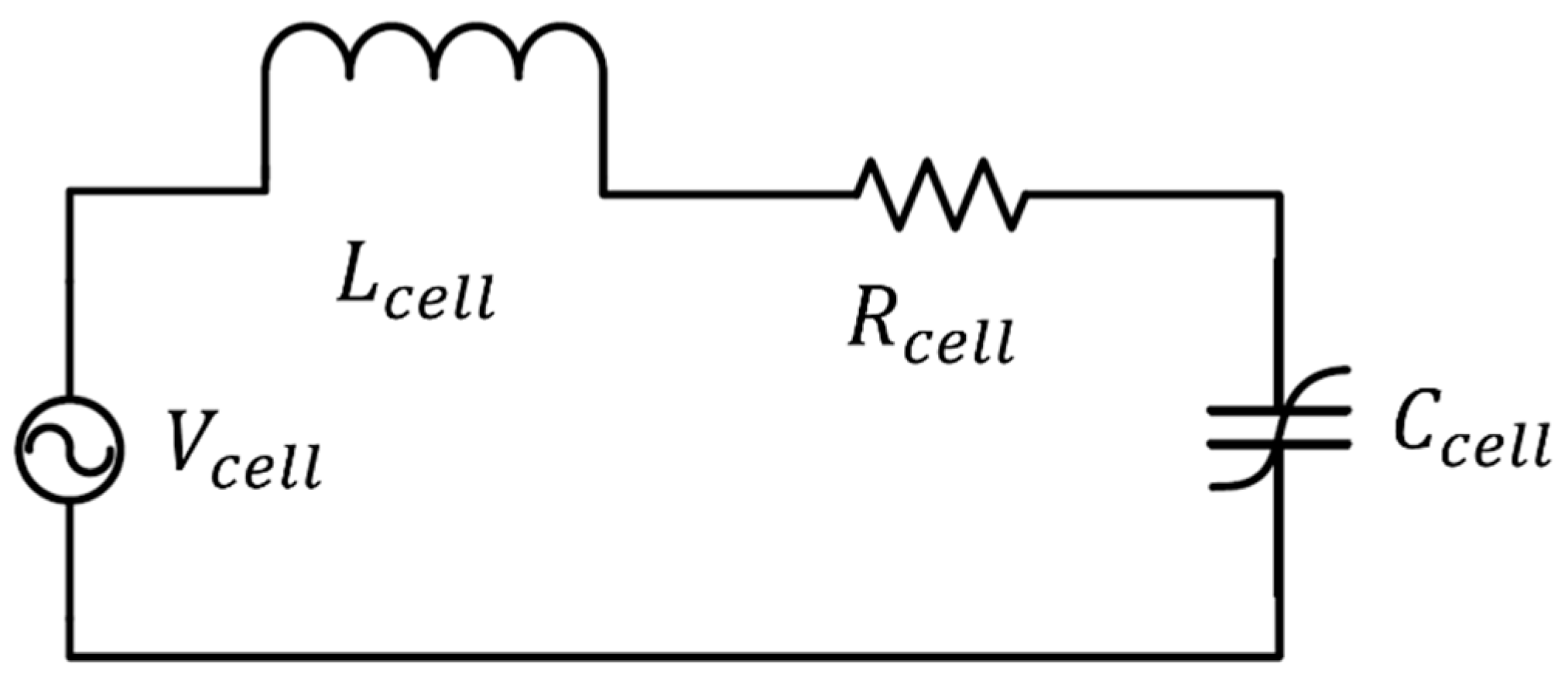
Most MTM-based MNG lenses presented in the literature to enhance the magnetic coupling between the IPT drivers are based on linear resonators consisting of a lattice of planar coils with resonance frequency controlled by a series-connected linear lumped or distributed capacitances [18]. In terms of equivalent impedance, these resonators can be represented as a simple series RLC circuit:

$$Z_{cell}=R_{cell}+j\omega L_{cell}+\frac{1}{j\omega C_{cell}}$$

(6)

where $R_{cell}$, $L_{cell}$, and $C_{cell}$ are the linear resistance, inductance, and capacitance of the MTM cell circuit.

The MTM capability of enhancing the power transmission between the drivers depends on its energy storing capacity, which, by definition, can be quantified by the Q-factor of the resonator:

$$Q_{cell}\triangleq \frac{Energy Stored}{Power Dissipated per Cycle}\cong \frac{{\omega }_0}{\mathsf{\Delta }\omega }$$

(7)

where ${\omega }_0$ is the resonance angular frequency and $\mathsf{\Delta }\omega$ is its half-power bandwidth.

The Q-factor can also be written as the ratio of the reactive impedance $\sqrt{\frac{L_{cell}}{C_{cell}}}$ and the resistive impedance $R_{cell}$:

$$Q_{cell}=\frac{1}{R_{cell}}\sqrt{\frac{L_{cell}}{C_{cell}}}$$

(8)

Knowing that ${\omega }_0=\frac{1}{\sqrt{L_{cell}{C}_{cell}}}$, the definition of $\mathsf{\Delta }\omega$ for any series RLC can then be obtained as:

$$\mathsf{\Delta }\omega =\frac{R_{cell}}{L_{cell}}=2\gamma$$

(9a)

$$\gamma \triangleq \frac{R_{cell}}{2L_{cell}}$$

(9b)

where $\gamma$ is the damping factor.

Based on (7)–(9), it can be concluded that for the linear case the amplitude-bandwidth characteristic of the system can only be improved by increasing ${\omega }_0$.

2.3. Nonlinear Series-Connected Unit Cell Based on Duffing Resonator

The basic and most common DR topology is a series-connected RLC with a nonlinear capacitance, as shown in Figure 5. As discussed in [14], in order to obtain a stable DR response, the circuit nonlinear capacitance must be symmetrical to the voltage bias:

$$C\left(v_C\right)=C\left(-v_C\right)$$

(10)

As discussed in [14,15], the DR’s behavior based on bias-symmetrical nonlinear components is dominated by its third-order nonlinear component, which results in the following differential equation:

$$\frac{d^2{q}_C\left(t\right)}{d{t}^2}+2\gamma \frac{d{q}_C\left(t\right)}{dt}+{\omega }_0^2{q}_C\left(t\right)+ϵq_C{\left(t\right)}^3=Ecos\left(\omega t\right)$$

(11)

where $q_C$ is the nonlinear capacitor charge, $E$ is the amplitude of the excitation applied to the system, $\omega$ is the angular frequency of the excitation, $\gamma$ is the damping coefficient, and $ϵ$ is the nonlinear coefficient. Notice that $ϵ=0$ represents the linear case, while $ϵ<0$ represents a nonlinear softening resonance obtained with a well-shaped C–V curve and $ϵ>0$ represents a hardening resonance obtained with bell-shaped C–V curve.

Utilizing the harmonic balance method, an approximation solution for the amplitude of the steady-state response of (11) as a function of $\omega$ can be found. First, the solution of $q_C\left(t\right)$ is assumed to be of the form:

$$q_C\left(\theta \right)=A_1\cos \left(\theta \right)+A_2\sin \left(\theta \right)=A\cos \left(\theta -\varphi \right)$$

(12a)

$$A^2\triangleq A_1^2+A_2^2$$

(12b)

$$\varphi \triangleq {\tan }^{-1}\frac{A_2}{A_1}$$

(12c)

where $A$ is the frequency-dependent amplitude of $q_C$, $\varphi$ is the frequency-dependent phase of $q_C$, and $\theta =\omega t$ is the normalized time.

Then (12) is replaced in (11):

$$\begin{array}{c}\left(-{\omega }^2{A}_1+2\omega \gamma A_2+{\omega }_0^2{A}_1+\frac{3}{4}ϵA_1^3+\frac{3}{4}ϵA_1{A}_2^2-E\right)\cos \left(\theta \right)\\ +\left(-{\omega }^2{A}_2-2\omega \gamma A_1+{\omega }_0^2{A}_2+\frac{3}{4}ϵA_2^3+\frac{3}{4}ϵA_1^2{A}_2\right)\sin \left(\theta \right)\\ +\left(\frac{1}{4}ϵA_1^3-\frac{3}{4}ϵA_1{A}_2^2\right)\cos \left(3\theta \right)+\left(\frac{3}{4}ϵA_1^2{A}_2-\frac{1}{4}ϵA_2^3\right)\sin \left(3\theta \right)=0\end{array}$$

(13)

Making the simplifying hypothesis that the amplitudes of the third-harmonic components are negligible, (13) imposes that the amplitudes of the fundamental-mode components are null:

$$-{\omega }^2{A}_1+2\omega \gamma A_2+{\omega }_0^2{A}_1+\frac{3}{4}ϵA_1^3+\frac{3}{4}ϵA_1{A}_2^2-E=0$$

(14a)

$$-{\omega }^2{A}_2-2\omega \gamma A_1+{\omega }_0^2{A}_2+\frac{3}{4}ϵA_2^3+\frac{3}{4}ϵA_1^2{A}_2=0$$

(14b)

Squaring both equations in (14) and adding them, the frequency response of the charge amplitude in DRs is found to be:

$$\left({\left({\omega }^2-{\omega }_{0,eq}^2\right)}^2+4{\gamma }^2{\omega }^2\right)A^2=E^2 \left(Amplitude relation\right)$$

(15a)

$$\varphi ={\tan }^{-1}\left(\frac{2\gamma \omega }{{\omega }^2-{\omega }_{0,eq}^2}\right) \left(Phase relation\right)$$

(15b)

$${\omega }_{0,eq}\triangleq \sqrt{{\omega }_0^2+\frac{3}{4}ϵA^2}$$

(15c)

Notice that for low amplitudes of $A$ or low $ϵ$, the DR becomes quasilinear (${\omega }_{0,eq}\approx {\omega }_0$). For that particular case and the linear one ($ϵ=0$), a closed-form solution for $A$ can be obtained from (15):

$$A=\pm \sqrt{\frac{E^2}{{\left({\omega }^2-{\omega }_0^2\right)}^2+4{\gamma }^2{\omega }^2}} \left[C\right]$$

(16)

where the different signs of (16) represent the possible polarities of the charge. By convention, $A$ is typically chosen to be positive although the electron has a negative charge.

Even though no closed-form solution can be obtained for the nonlinear case, (15) can still be solved for ($ϵ\ne 0$) by expanding it as a six-order polynomial in terms of a variable $A$:

$$\frac{9}{16}{ϵ}^2{A}^6+\frac{3}{2}ϵ({\omega }_0^2-{\omega }^2)A^4+({({\omega }^2-{\omega }_0^2)}^2+4{\gamma }^2{\omega }^2)A^2-E^2=0$$

(17)

where each root of (17) represents a state solution of (11). Since (17) is an even function and is symmetrical to $A$, there are only three independent solutions (charge states). If $A_1$, $A_2$, and $A_3$ are the positive roots of (17), and $A_{-1}$, $A_{-2}$, and $A_{-3}$ are its negative roots, then they are related as follows:

$$\begin{array}{c}{A}_1=-A_{-1}\\ A_2=-A_{-2}\\ A_3=-A_{-3}\end{array}$$

(18)

Like in the linear case in (16), the positive and negative pairs of independent solutions of (17) reflect the choice of the charge polarity. Notice that (17) becomes (16) if $ϵ=0$. So, keeping the positive sign convention for the charge, we can ignore the negative roots.

For a given set of $E, \omega , {\omega }_0, \gamma$ and $ϵ$, $A_1$, $A_2$, or $A_3$ represent stable states solutions of (11) if and only if they are real numbers. Since there is an odd number of roots on the positive $A$-axis, at least one of them is a real number.

Since the only nonlinear element in the DR is its capacitance, it is reasonable to admit that ${\omega }_0$ and $ϵ$ are given by:

$${\omega }_0=\frac{1}{L_{cell}{a}_1}$$

(19a)

$$ϵ=\frac{1}{L_{cell}{a}_3}$$

(19b)

where $L_{cell}$ is the DR linear inductance, and $a_1$ and $a_3$ are the DR linear and nonlinear capacitances.

Based on (17), ${\omega }_{0,eq}$ can now be rewritten as:

$${\omega }_{0,eq}=\sqrt{\frac{1}{L_{cell}}\left(\frac{1}{a_1}+\frac{\frac{3}{4}{A}^2}{a_3}\right)}=\frac{1}{\sqrt{L_{cell}{C}_{cell,eq}}}$$

(20a)

$$C_{cell,eq}\triangleq \frac{a_1{a}_3}{a_3+\frac{3}{4}{A}^2{a}_1}$$

(20b)

2.4. Criterium to Determine the Bandwidth Enhancement

Since no straight relationship between resonance amplitude and bandwidth can be derived for the DR as the one found in (7), its bandwidth enhancement capabilities must be investigated by comparing it with the linear limit.

First, a normalized amplitude-bandwidth limit for the linear case ($ϵ=0$) must be defined. Substituting (7) and (9) into (16), the maximum achievable charge amplitude $A_0$ for the linear case is obtained at ${\omega }_0$:

$$A_0\mathsf{\Delta }{\omega }_0=\frac{E}{{\omega }_0}$$

(21)

where $\mathsf{\Delta }{\omega }_0$ is the linear half-power bandwidth.

Based on (21), when normalized by its own $A_0$ and $\mathsf{\Delta }{\omega }_0$, for any chosen set of parameters, the linear fundamental limit becomes simply:

$$A_{0,n}\mathsf{\Delta }{\omega }_{0,n}=1$$

(22)

From (11), the response of the DR can be described as the superposition of its linear (small signal) and nonlinear (large signal) terms. If the maximum nonlinear amplitude $A_1$ and maximum nonlinear half-power bandwidth $\mathsf{\Delta }{\omega }_1$ of any system described by (15) is normalized by its own linear maximum amplitude $A_0$ and bandwidth $\mathsf{\Delta }{\omega }_0$:

$$A_n\triangleq \frac{A_1}{A_0}$$

(23a)

$$\mathsf{\Delta }{\omega }_n\triangleq \frac{\mathsf{\Delta }{\omega }_1}{\mathsf{\Delta }{\omega }_0}$$

(23b)

Then the amplitude-bandwidth limit enhancement can be defined as:

$$A_n\mathsf{\Delta }{\omega }_n\triangleq \delta$$

(24)

where $\delta$ is the nonlinear gain. Notice that almost linear scenarios, $A_1\approx A_0$ and $\mathsf{\Delta }{\omega }_1\approx \mathsf{\Delta }{\omega }_0$, result in $A_n\mathsf{\Delta }{\omega }_n=1$, which is precisely the curve described by (22).

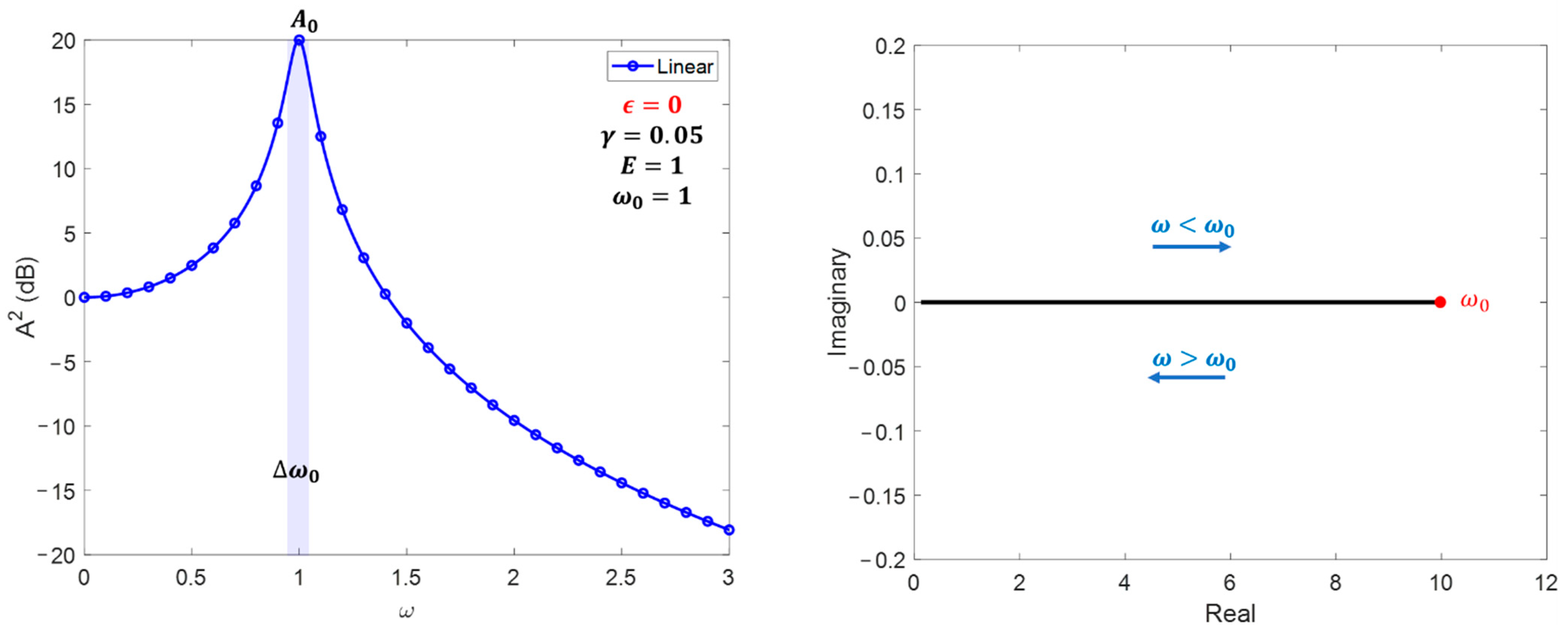
2.5. Numerical Examples for the Nonlinear Case

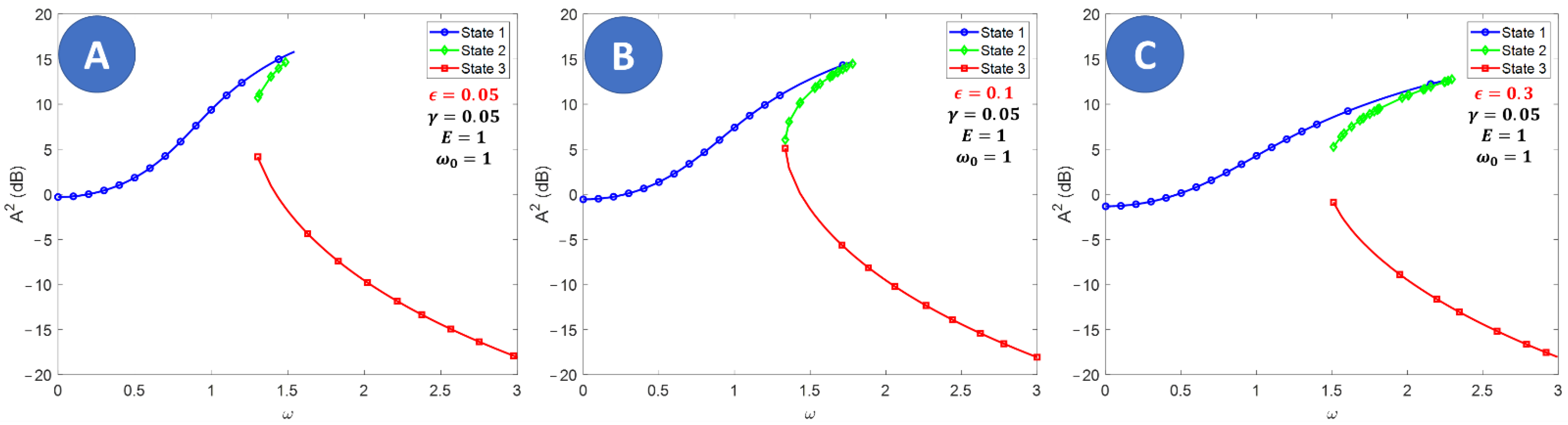
For the numerical example, let us consider a particular system characterized by $\gamma =0.05$, $E=1$, and ${\omega }_0=1$. As shown in Figure 6, for $ϵ=0$, there is only a one-state solution, and the maximum amplitude is obtained at ${\omega }_0$. 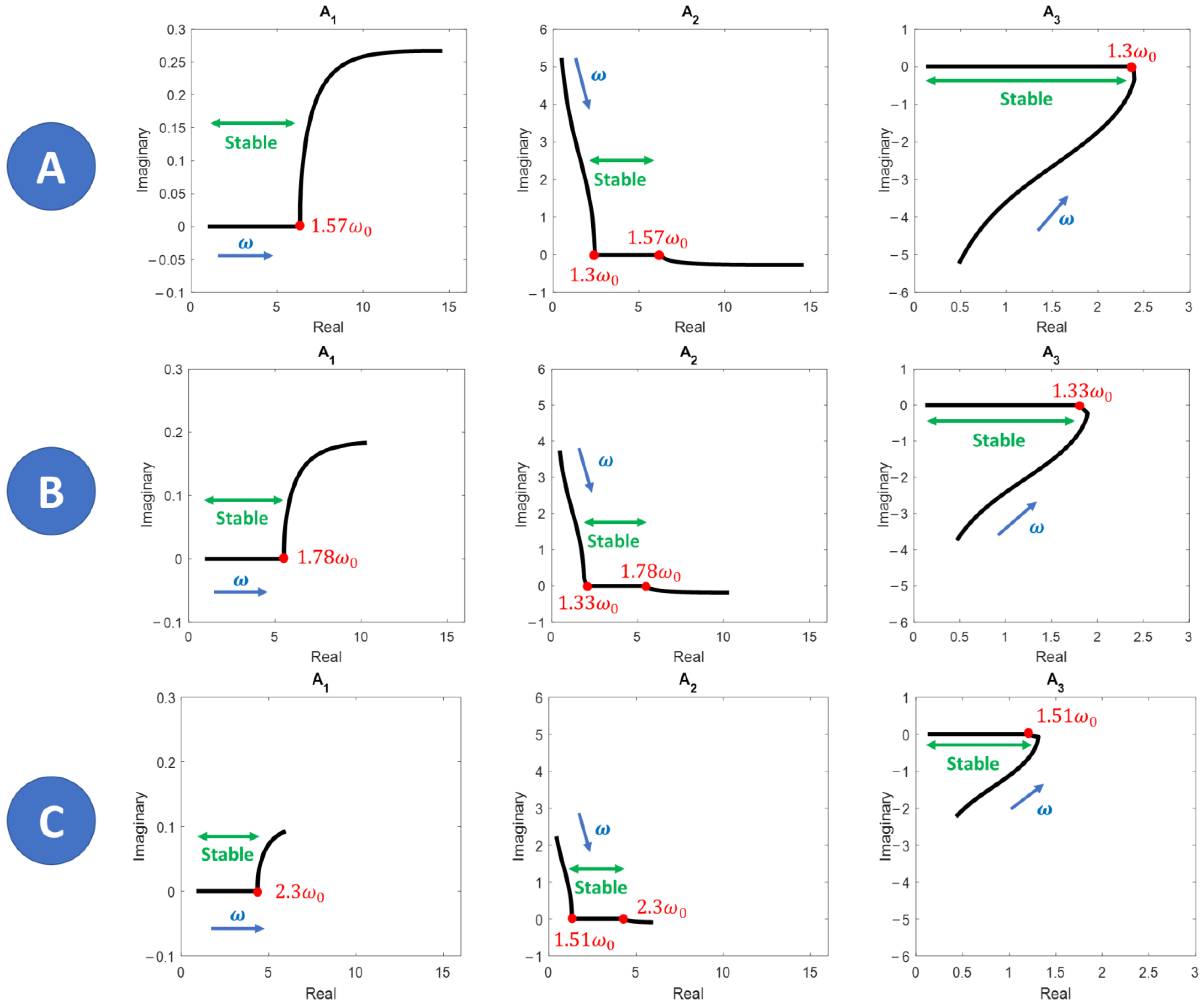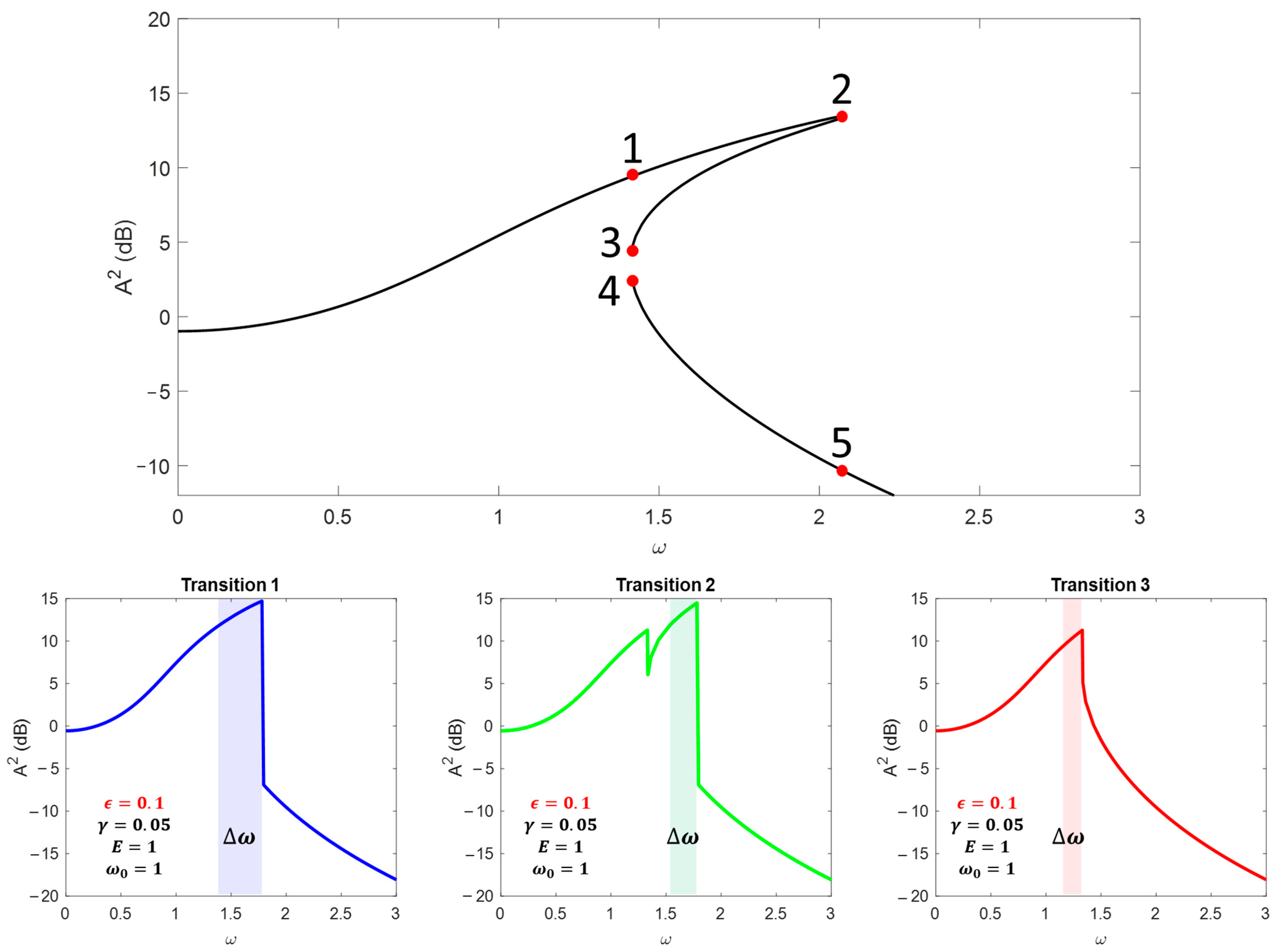However, when $ϵ>0$, the resonance hardening tilts the resonance peak to the right and the maximum amplitude is obtained $\omega >{\omega }_0$, as stated by (20) (see Figure 7). Due to the resonance hardening, three possible states exist for the resonator, although they are only stable in the frequency region where they are pure real numbers (see Figure 8). Around the nonlinear resonance ${\omega }_{0,eq}$, all three states become stable. Due to the multistability, the system can experience three different transitions between its stable solutions, leading to three possible amplitude-bandwidth characteristics for the system, as shown in Figure 9. Notice that the half-power bandwidth for $ϵ\ne 0$ is asymmetrical in relation to its maximum amplitude, so it is defined as the frequency range with $A^2\ge \frac{A_{MAX}^2}{2}$.

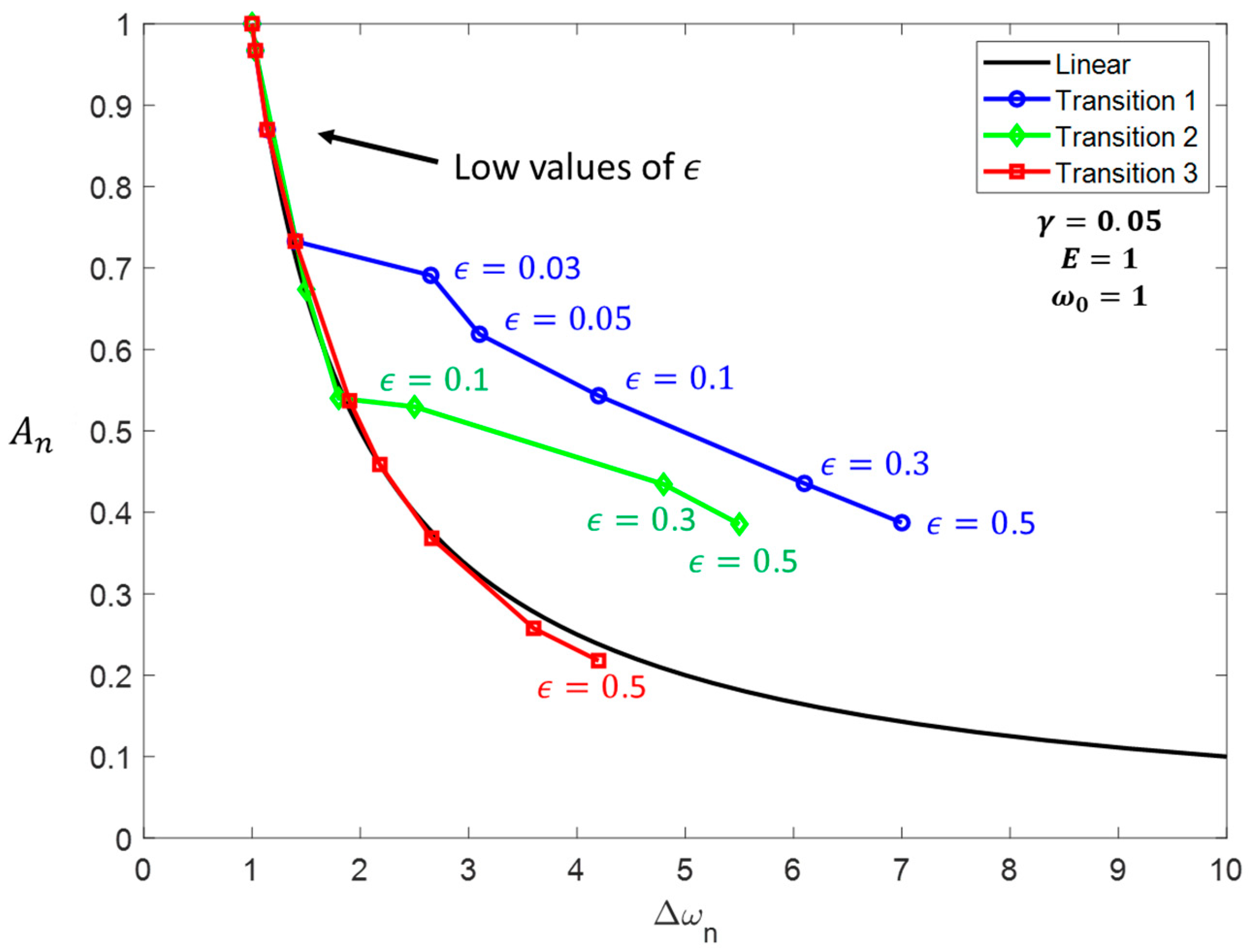
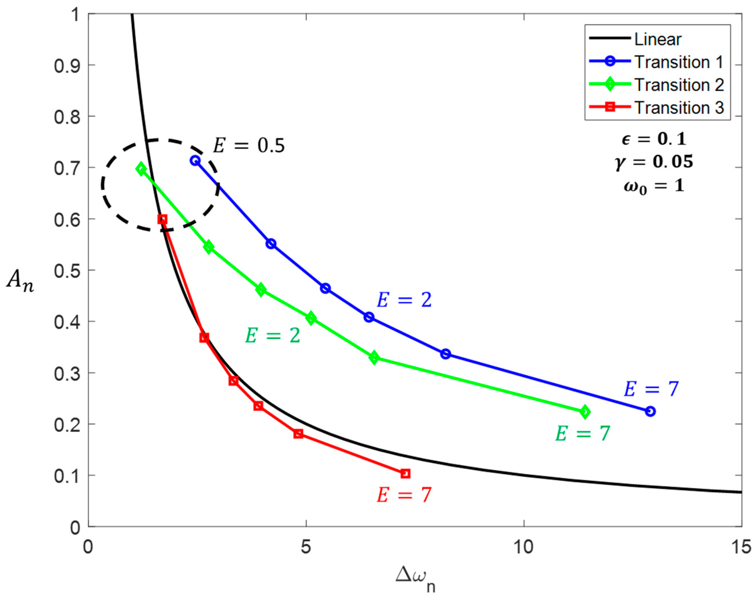
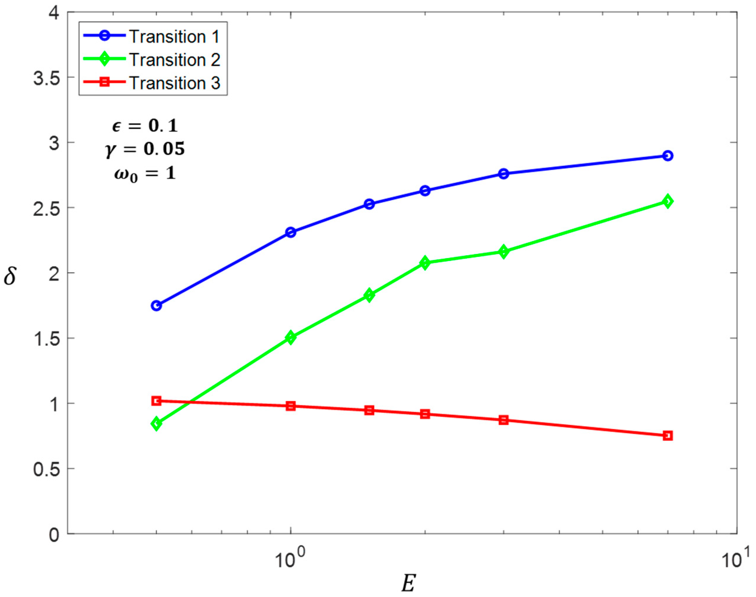
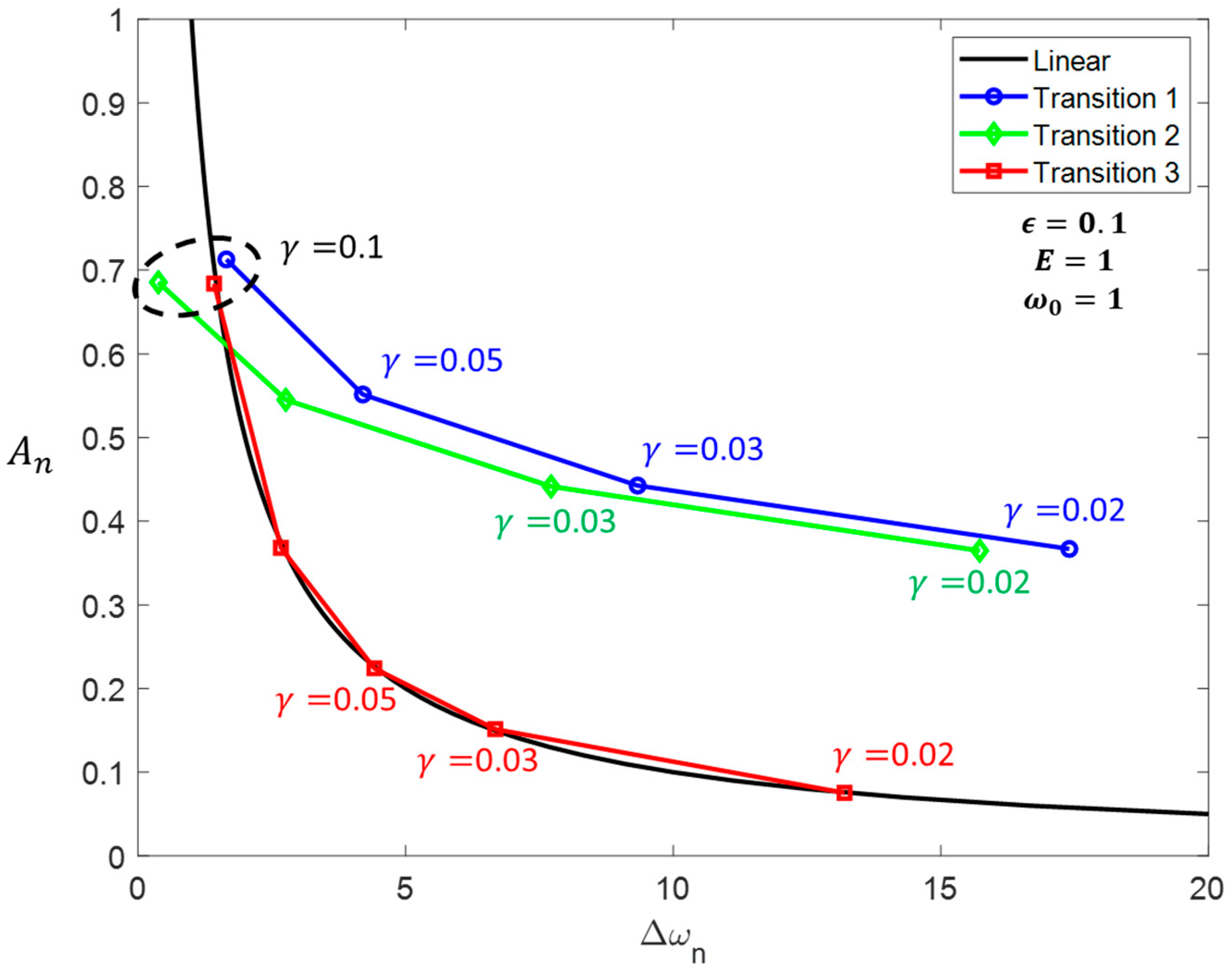
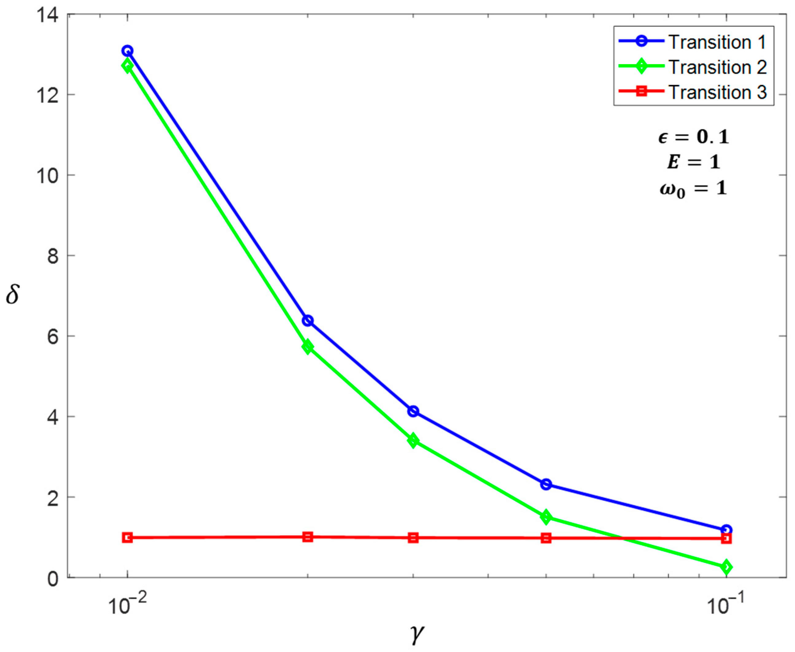
Using the criteria established in (21)–(24), the bandwidth enhancement capabilities for the three DR transitions can be determined by any chosen $E$, $ϵ$, and $\gamma$. As shown in Figure 10, Figure 11, Figure 12, Figure 13, Figure 14 and Figure 15, transitions 1 and 2 enhance the linear amplitude-bandwidth limit of the series-connected DR significantly. Nonetheless, if the system experiences transition 3 instead, the obtained amplitude-bandwidth limit is bounded by the linear case. Notice that for $\mathsf{\Delta }{\omega }_n<1.4$, the response obtained by any considered transition behaves similarly to the linear case. Especially for low values of $E$ and high values of $\gamma$, the nonlinear response can be even worse than the linear one. Finally, for high values of $ϵ$ and $E$, transitions 1 and 2 tend to behave similarly.

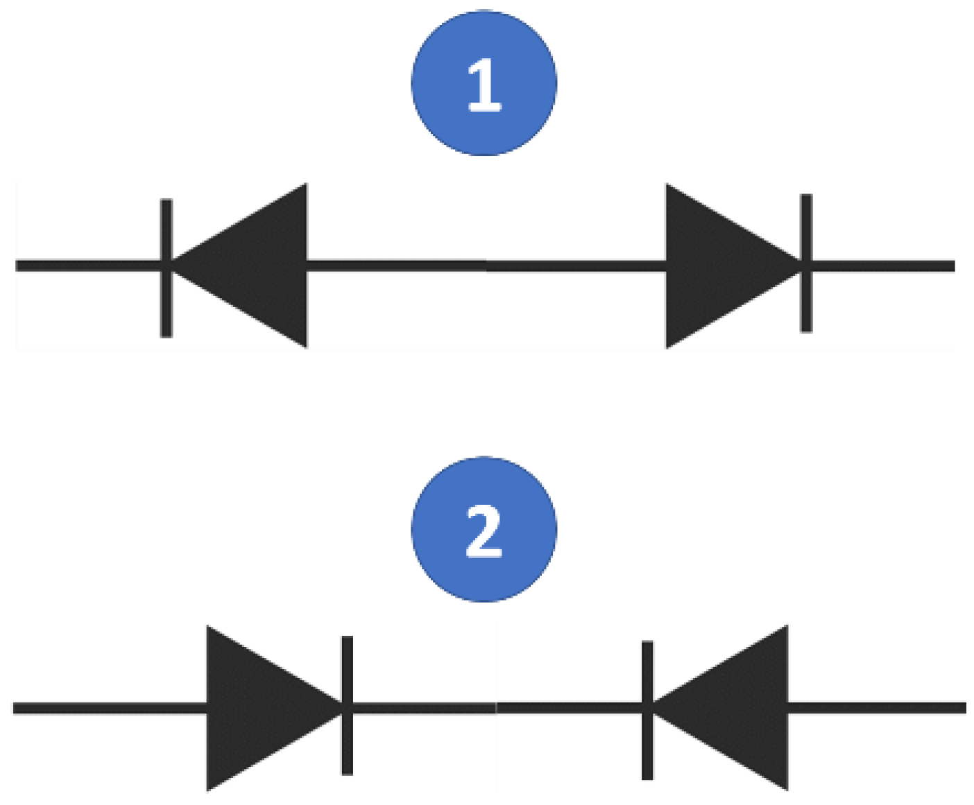
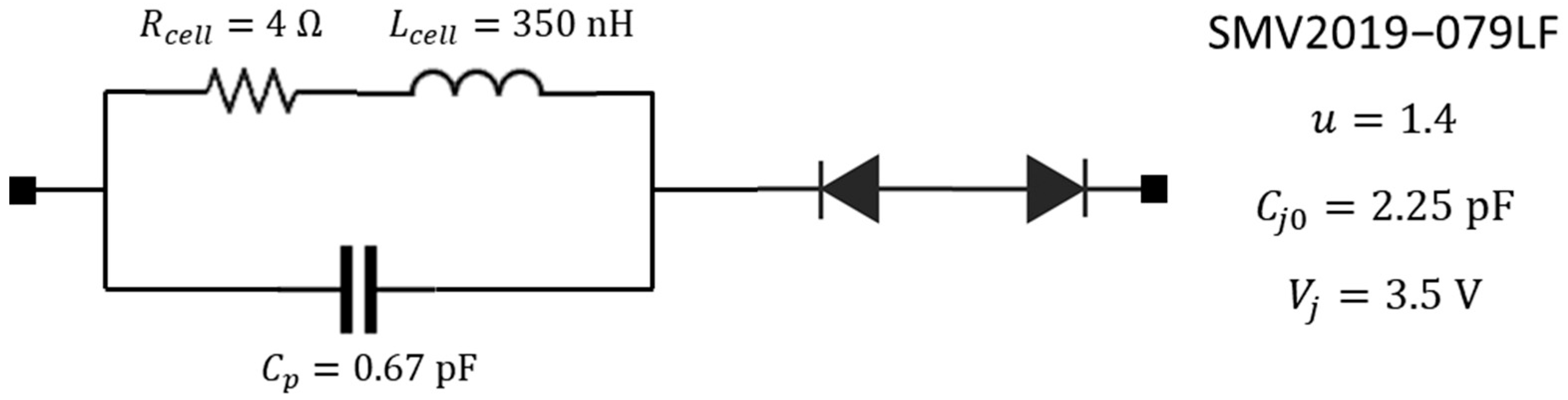
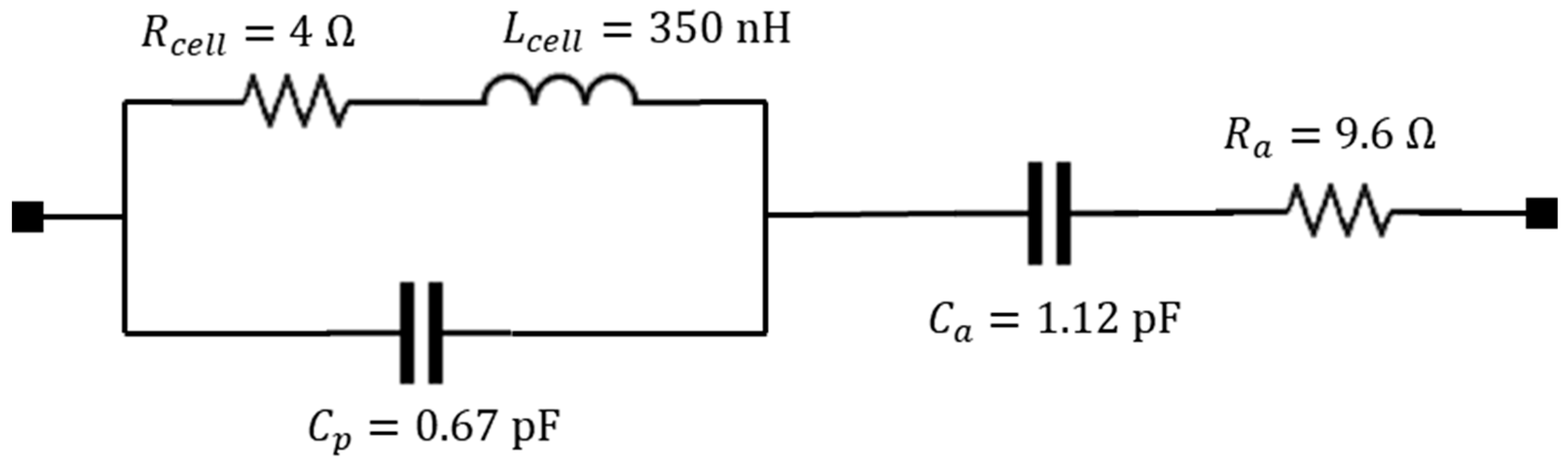
2.6. Duffing Resonance Implementation with a Pair of Varactors

As discussed in [19], a capacitor with a bell-shaped C–V curve can be implemented by a pair of varactor diodes connected in antiseries, as shown in Figure 16.

Neglecting the package parasitic capacitances, the capacitance of each varactor as a function of the applied reversed bias voltage $V_C$ is described by:

$$C_{diode}\left(V_C\right)=\frac{C_{j0}}{{\left(1+\frac{V_C}{V_j}\right)}^u}$$

(25)

where $C_{j0}$ is the junction capacitance, $V_j$ is the built-in junction voltage, and $u$ is the grading coefficient.

Expending (25) as a Maclaurin series and ignoring the terms higher than second-order, $C_{diode}$ can be approximated as:

$$C_{diode}\left(V_C\right)\approx k_0+k_1{V}_C+k_2{V}_C^2$$

(26a)

$$k_0=C_{j0}$$

(26b)

$$k_1=-C_{j0}\frac{u}{V_j}$$

(26c)

$$k_2=C_{j0}\frac{u\left(u+1\right)}{2V_j^2}$$

(26d)

Knowing that $V_{C1}$ and $V_{C2}$ are the voltage applied to the diodes of the antiseries, the charge stored in each of them according to (26) is then:

$$Q_{C1}={{\displaystyle \int }}_0^{V_{C1}}{C}_{diode}\left(V_C\right)d{V}_C=k_0{V}_{C1}-\frac{k_1}{2}{V}_{C1}^2+\frac{k_2}{3}{V}_{C1}^3$$

(27a)

$$Q_{C2}={{\displaystyle \int }}_0^{V_{C2}}{C}_{diode}\left(V_C\right)d{V}_C=k_0{V}_{C2}+\frac{k_1}{2}{V}_{C2}^2+\frac{k_2}{3}{V}_{C2}^3$$

(27b)

Notice that there is a sign change in the second-order term of $Q_{C1}$ and $Q_{C2}$ due to the antiseries configuration, which changes the relative sign of $V_j$ for each diode.

Reversing (27), the expressions of $V_{C1}$ and $V_{C2}$ in terms of their charges become:

$$V_{C1}=\frac{Q_{C1}}{k_0}-\frac{k_1}{2k_0^3}{Q}_{C1}^2+\frac{1}{k_0^5}\left(\frac{k_1^2}{2}-\frac{k_0{k}_2}{3}\right)Q_{C1}^3$$

(28a)

$$V_{C2}=\frac{Q_{C2}}{k_0}+\frac{k_1}{2k_0^3}{Q}_{C2}^2+\frac{1}{k_0^5}\left(\frac{k_1^2}{2}-\frac{k_0{k}_2}{3}\right)Q_{C2}^3$$

(28b)

If the diodes are identical, then the total voltage $V_C$ applied to the antiseries pair:

$$V_C=V_{C1}+V_{C2}=\frac{2}{k_0}{Q}_C+\frac{2}{k_0^5}\left(\frac{k_1^2}{2}-\frac{k_0{k}_2}{3}\right)Q_C^3$$

(29a)

$$Q_C=Q_{C1}=Q_{C2}$$

(29b)

By dimensional analysis of (29), the linear and nonlinear capacitances of the DR defined in (19) are found to be:

$$a_1=\frac{k_0}{2}=\frac{C_{j0}}{2}$$

(30a)

$$a_3=\frac{k_0^5}{2\left(\frac{k_1^2}{2}-\frac{k_0{k}_2}{3}\right)}=\frac{3V_j^2{C}_{j0}^3}{16u\left(5u-1\right)}$$

(30b)

Based on (19) and (30), the linear resonance frequency ${\omega }_0$ and the nonlinear coefficient $ϵ$ in (11) can be written in terms of the circuit and diode parameters only:

$${\omega }_0=\sqrt{\frac{2}{L_{cell}{C}_{j0}}}$$

(31a)

$$ϵ=\frac{16u\left(5u-1\right)}{3L_{cell}{V}_j^2{C}_{j0}^3}$$

(31b)

Notice in (31) that the antiseries pair of varactors always conduct to $ϵ>0$ (hardening resonance) since $u\ge 1$. Knowing that its dimension is volts per henry, the excitation $E$ can also be rewritten in terms of the cell parameters as:

$$E=\frac{V_{cell}}{L_{cell}}$$

(32)

where $V_{cell}$ is the voltage induced to the cell by the TX coil.

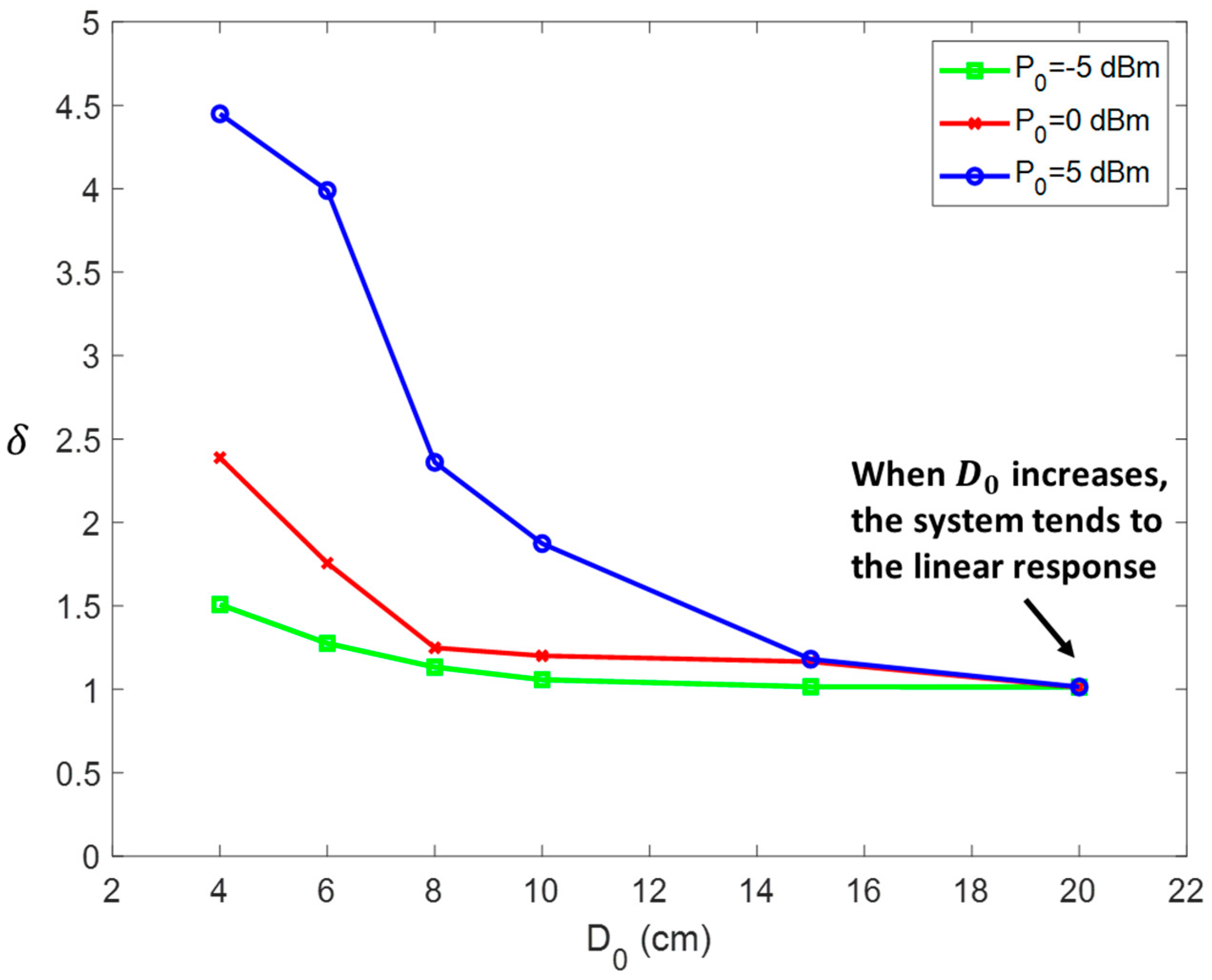
Notice that since $V_{cell}$ depends on both the H-field intensity and the coupling between the TX coil and the MTM cells, the response of the nonlinear MTM will vary as a function of the TX input power and the separation distance between the lens and the TX coil. However, in practical applications, the MTM is supposed to be as close as possible to the TX driver to minimize the TX profile and their relative positions do not change. Thus, coupling between these two is sufficiently high and constant when the IPT system is operating.

3. Results and Discussion

3.1. Proposed Nonlinear MTM Lens

Based on the results found in Section 2, a simple DR unit cell can be obtained by connecting a conventional planar spiral resonator in series with a nonlinear pair of varactors. The proposed nonlinear cell is shown in Figure 17. The design is built on RO3003. The considered substrate and copper thicknesses are $1 \mathrm{mm}$ and $17 \mathsf{\mu }\mathrm{m}$, respectively. The nonlinear capacitance is obtained with two SMV2019-079LF diodes connected in antiseries. The large-signal SPICE model of the diodes was obtained from the datasheet provided by the manufacturer.

The proposed nonlinear unit cell can be approximated by the circuit model shown in Figure 18. Notice that $C_p$ accounts for the parasitic capacitance of the planar coil. The equivalent linear cell is obtained from the small-signal response of the SPICE model. For small signals, the antiseries diodes behave like a simple series-connected RC circuit, as shown in Figure 19.

3.2. Numerical Simulations of the Proposed Lens

For the numerical simulations, the considered system configuration is the same one presented in Figure 2 (coaxial configuration), with $D=8 \mathrm{cm}$, $\mathsf{\Lambda }=2.3 \mathrm{cm}$, $N_x=N_y=4$, and $D_{TX-MTM}=D_0/2$. $P_0$ is the input power of the source connected to the TX coil. $P_{cell}$ is the average power delivered to the MTM cells. The simulations were done with Keysight Pathwave ADS 2021, using circuit and full-wave co-simulation. The full-wave simulation of the TX and RX coils and the MTM slab employed the Method of Moments (MoM) solver, while the large-signal circuit simulation of the entire system, including the diodes, employed the harmonic balance method. Since the considered structure is planar, the MoM was chosen instead of the Finite Element Method (FEM) solver to reduce the overall simulation time.

As shown in Figure 20, Figure 21, Figure 22 and Figure 23, differently to the linear MTM, which depends on the magnetic coupling ${\kappa }_m$ between TX and RX (and consequently $D_0$) but is almost insensitive to $P_0$, the proposed nonlinear MTM response varies with both. This is an expected result since a minimum power delivered to the cells $P_{cell}^{min}$ is required in order to activate the cells’ nonlinear response. Consequently, at each operating distance $D_0$, there will be a different $P_0$ threshold to be achieved in order to provide $P_{cell}^{min}$ to the cells and obtain a non-negligible nonlinear gain $\delta$ for the system. In the considered scenario of a lens located at $D_{TX-MTM}=D_0/2$, the nonlinear enhancement of the amplitude-bandwidth limit is strong only for $D_0<D$. For $D_0>D$, ${\kappa }_m$ becomes too small, meaning an extremely high $P_0$ would be needed in order to deliver enough power to the cells to surpass $P_{cell}^{min}$. For example, considering $D_0=6 \mathrm{cm}$, the nonlinear response is almost negligible if $P_0<-5 \mathrm{d}\mathrm{B}\mathrm{m}$, and the resonance hardening is apparent only if $P_0>0 \mathrm{d}\mathrm{B}\mathrm{m}$ (see Figure 20).

As shown in Figure 21, for $D_0<D$ and $P_0>0 \mathrm{d}\mathrm{B}\mathrm{m}$, very high $\delta$ can be obtained (about 4.5 times), while for $D_0\gg D$ and/or very low $P_0$, $\delta$ tends to 1 (linear case). Due to the MTM gain attenuation caused by strongly coupled TX and RX coils, maximum gain and maximum bandwidth are obtained for different $D_0$ values (see Figure 22). Concerning the MTM gain attenuation due to TX–RX strong coupling, the phenomenon was already explained in Section 2.1 for the linear case using (5).

As shown in Figure 23, when $P_{cell}$ is high enough to trigger the resonance hardening, due to the increasing of $P_0$ and/or the reduction of $D_0$, the nonlinear MTM can almost double the PTE in relation to its equivalent linear one. Considering all the results presented in Figure 21, Figure 22 and Figure 23, in a short operating distance range ($D_0<D$), even when $P_0=-5 \mathrm{d}\mathrm{B}\mathrm{m}$, the proposed nonlinear MTM can slightly outperform its linear equivalent one. Nonetheless, the considered configuration has presented an upper limit for $P_0$. When $P_0>5 \mathrm{d}\mathrm{B}\mathrm{m}$ and $D_0$ is short, the collective behavior of the nonlinear cells becomes unstable and $\delta$ deteriorates. When $P_{cell}$ becomes too high and resonance hardening is too strong, harmonic generation becomes increasingly important at the MTM cells’ circuitry level. Since MTM gain is proportional to the power stored in the cells at the fundamental mode, high harmonic power conversion limits its maximum achievable amplitude. Due to the existence of these lower and upper boundaries, the considered configuration has presented a significant, stable, improved performance in comparison to the linear case for $P_0=\left[-5 \mathrm{dBm}, 5 \mathrm{dBm}\right]$ and $D_0\le D$.

At last, notice that since PTE depends on both ${\kappa }_m$ and MTM gain, and ${\kappa }_m$ power transfer mechanism is dominant over the MTM one (obtained via the magnetic flux focusing), the maximum PTE is obtained for the shortest $D_0$ value, not for the $D_0$ that maximizes the MTM gain. Finally, notice that, in Figure 20, the resonance hardening significantly reduces the MTM loss region. Therefore, based on these preliminary results, the use of a nonlinear MTM lens with improved bandwidth characteristics seems feasible inside the appropriate $D_0$ and $P_0$ ranges. In any case, further studies are also required in order to confirm the presented results experimentally and to determine the most appropriate diode candidates to achieve maximum bandwidth enhancement with minimum PTE degradation for different operating temperatures, as has been done in [20,21,22].

4. Conclusions

This paper has presented the preliminary results on MNG MTM lenses using DR-based unit cells. For the first time, a criterium has been proposed to quantify and evaluate the amplitude-bandwidth enhancement due to the DR nonlinear response. According to the obtained theoretical and numerical results, at the center of the inductive link, the proposed nonlinear MTM lens could outperform an equivalent linear one in both maximum MTM gain and half-power bandwidth for operating distances no longer than the driver coils’ diameter and input power level between $-5 \mathrm{dBm}$ and $5 \mathrm{dBm}$. In short operating distances, if the input power is lower than $-5 \mathrm{dBm}$, the amplitude of the cells’ current (or charge distribution) is too small and the lens behavior tends to the linear case. Above $5 \mathrm{dBm}$, nonlinear gain starts to deteriorate as the input power increases due to strong harmonic generation, meaning that there is an optimal range for the power delivered to the cells. In the appropriate operating power and distance range, the nonlinear response can not only improve the amplitude-bandwidth limit of the MTM lens but also mitigate the MTM loss region. These findings imply that nonlinear lenses could potentially become a good alternative for applications with short operating distances and requiring simultaneous power and data transmission, such as CBS for electronics and/or implanted devices and body sensors, if the presented numerical results are confirmed by experimental studies.