Time- and Frequency-Domain Steady-State Solutions of Nonlinear Motional Eddy Currents Problems


Abstract
1. Introduction
2. Modeling
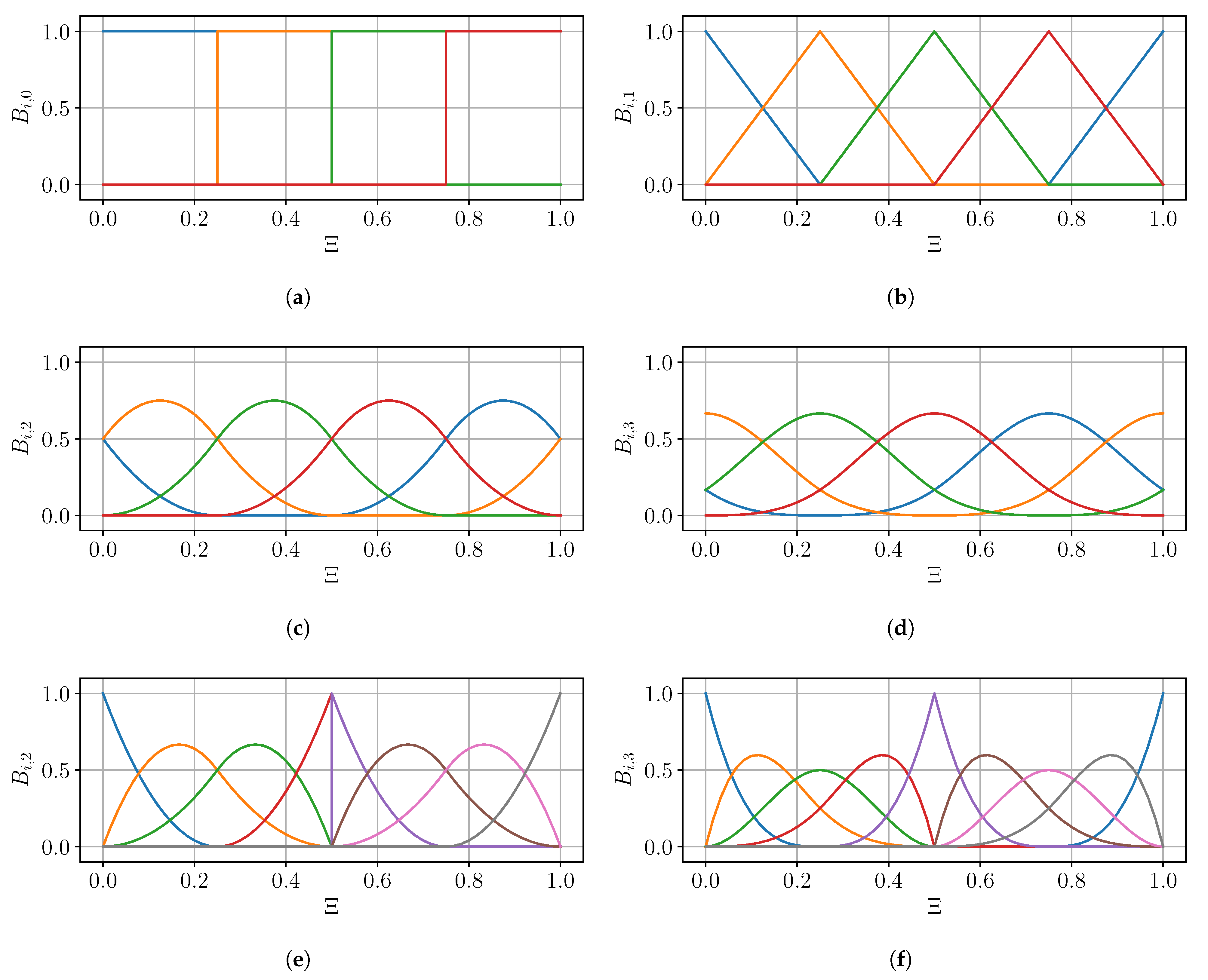
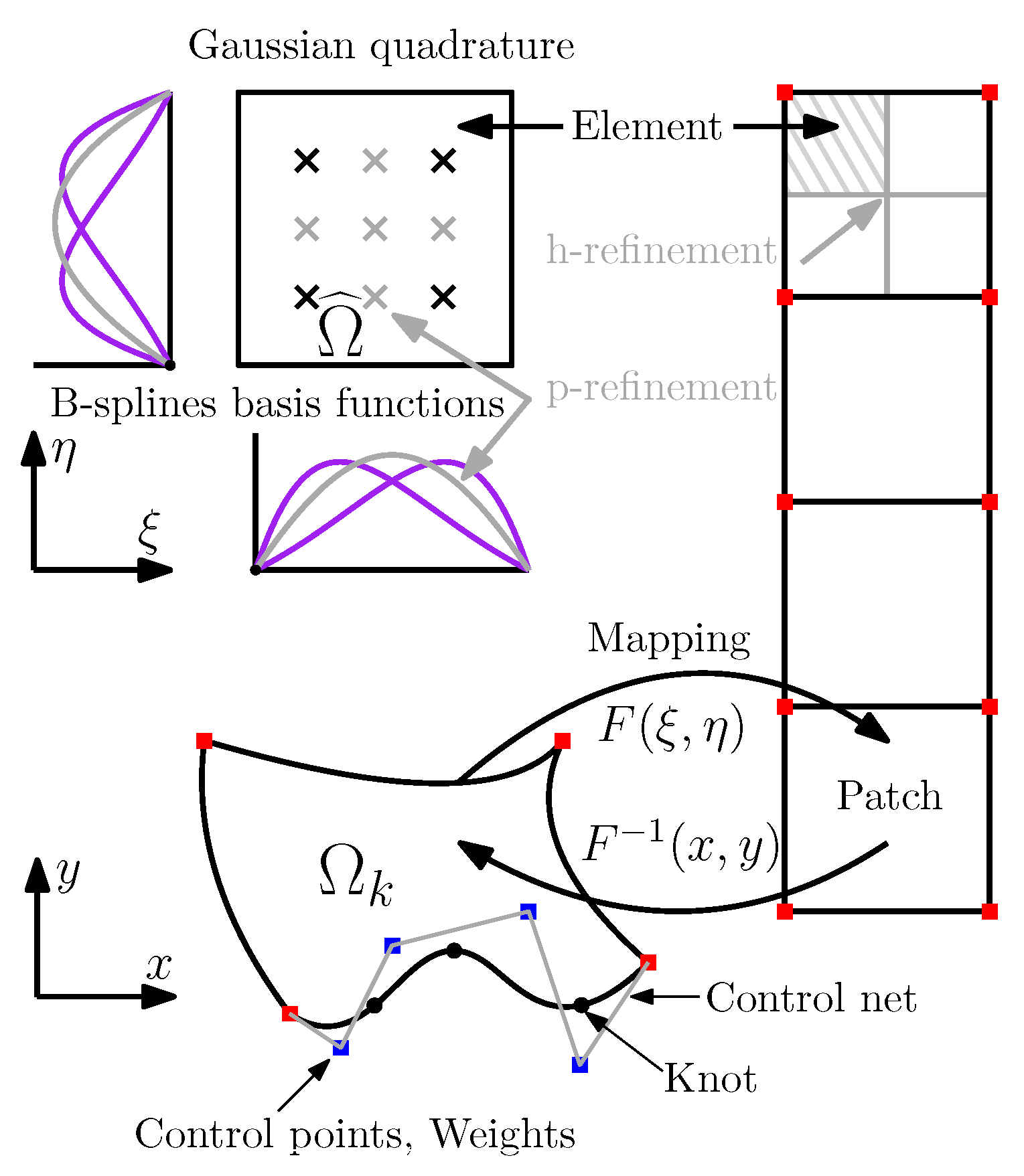
2.1. Isogeometric Analysis
2.2. Spatial Discretization of Nonlinear Magnetic Problems
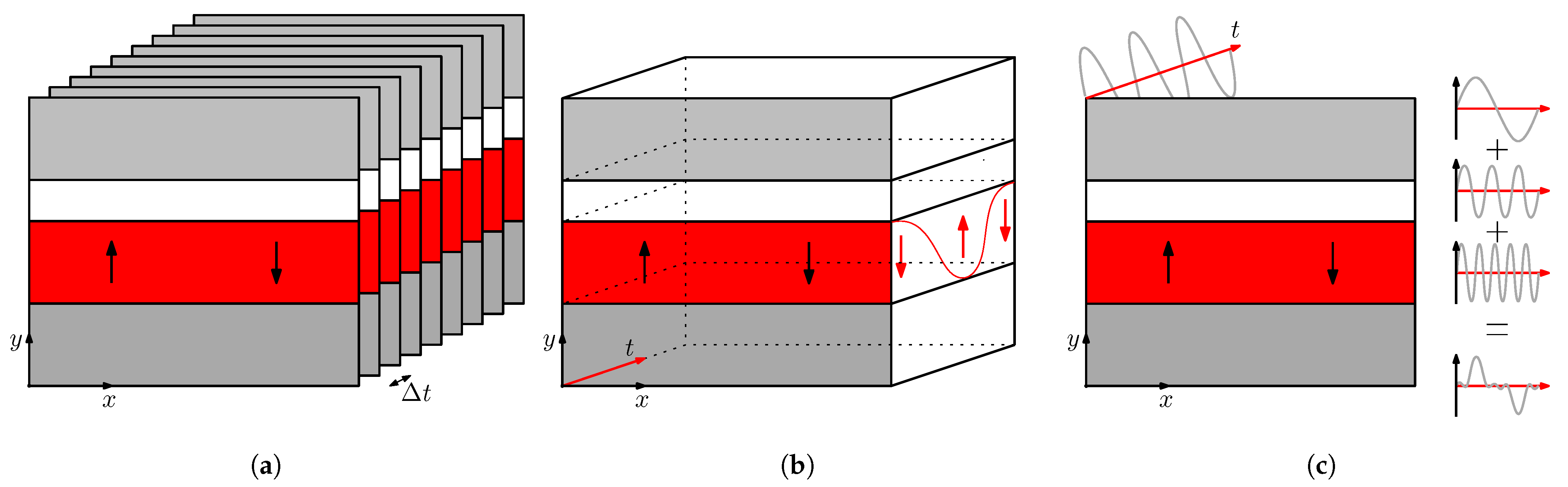
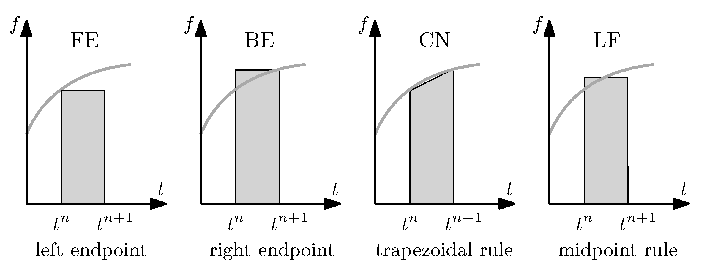
2.3. Time-Stepping Technique
2.4. Harmonic Balance Method
2.5. Space-Time Galerkin Approach
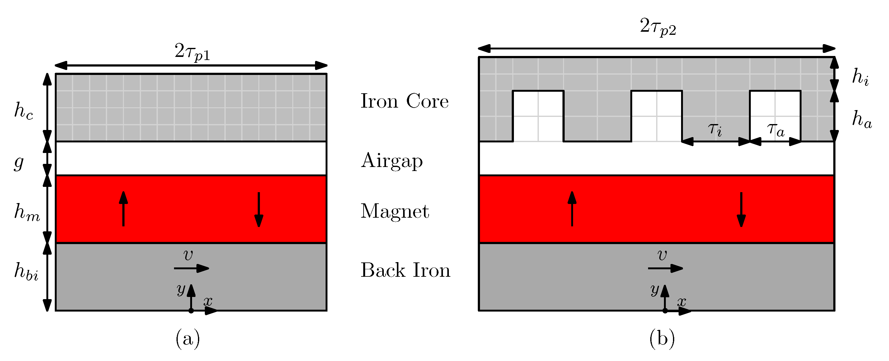
2.6. Benchmarks
3. Results
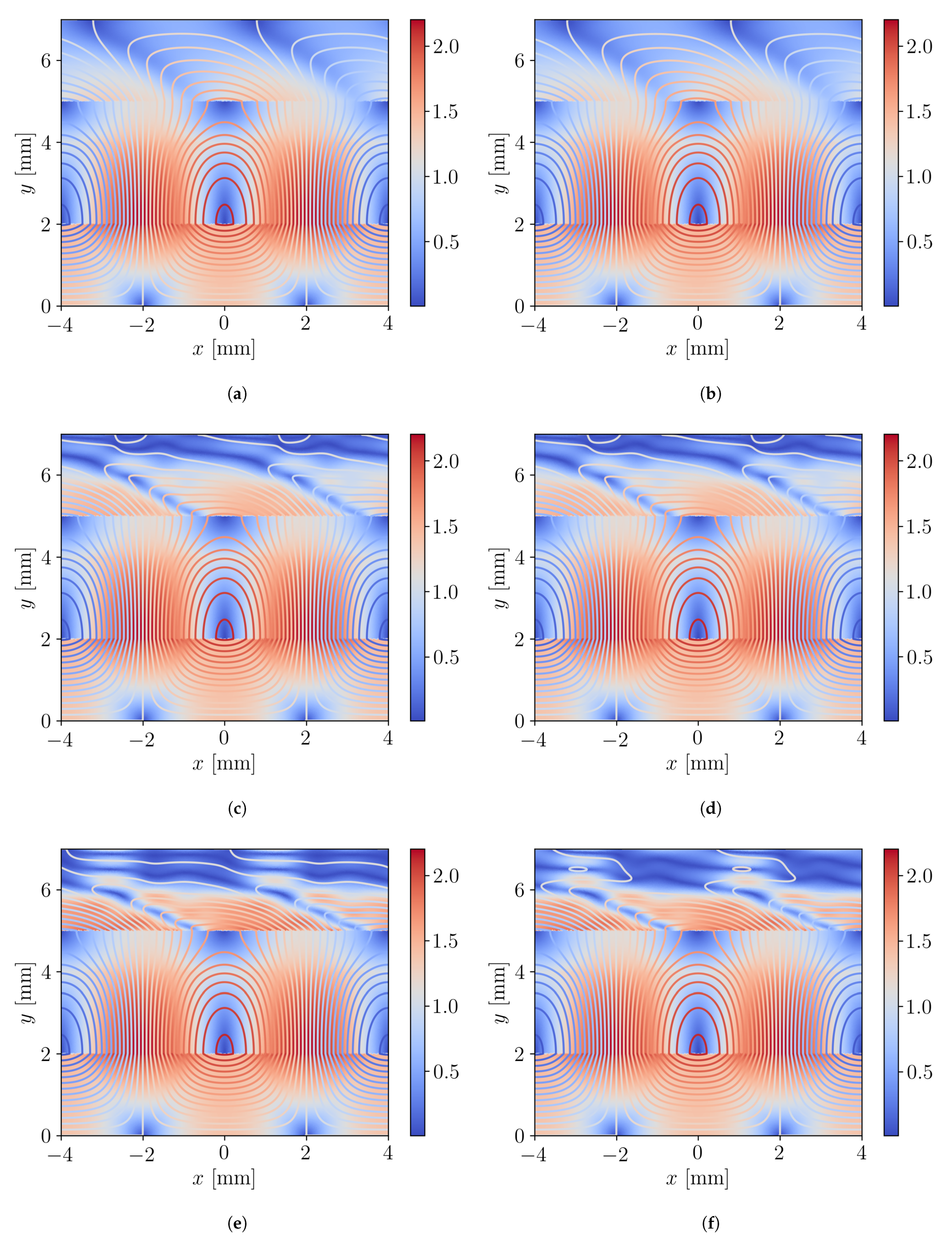
3.1. Slotless Benchmark
3.2. Slotted Benchmark
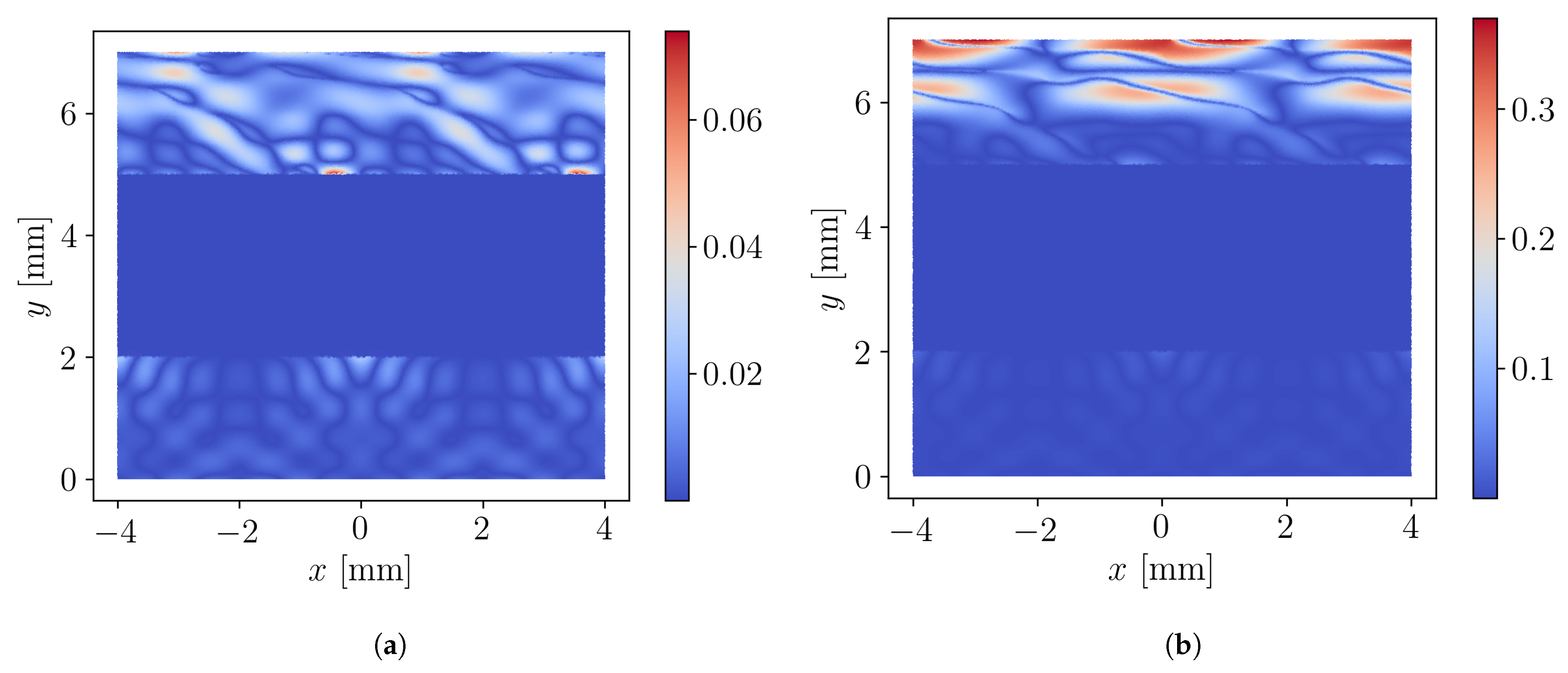
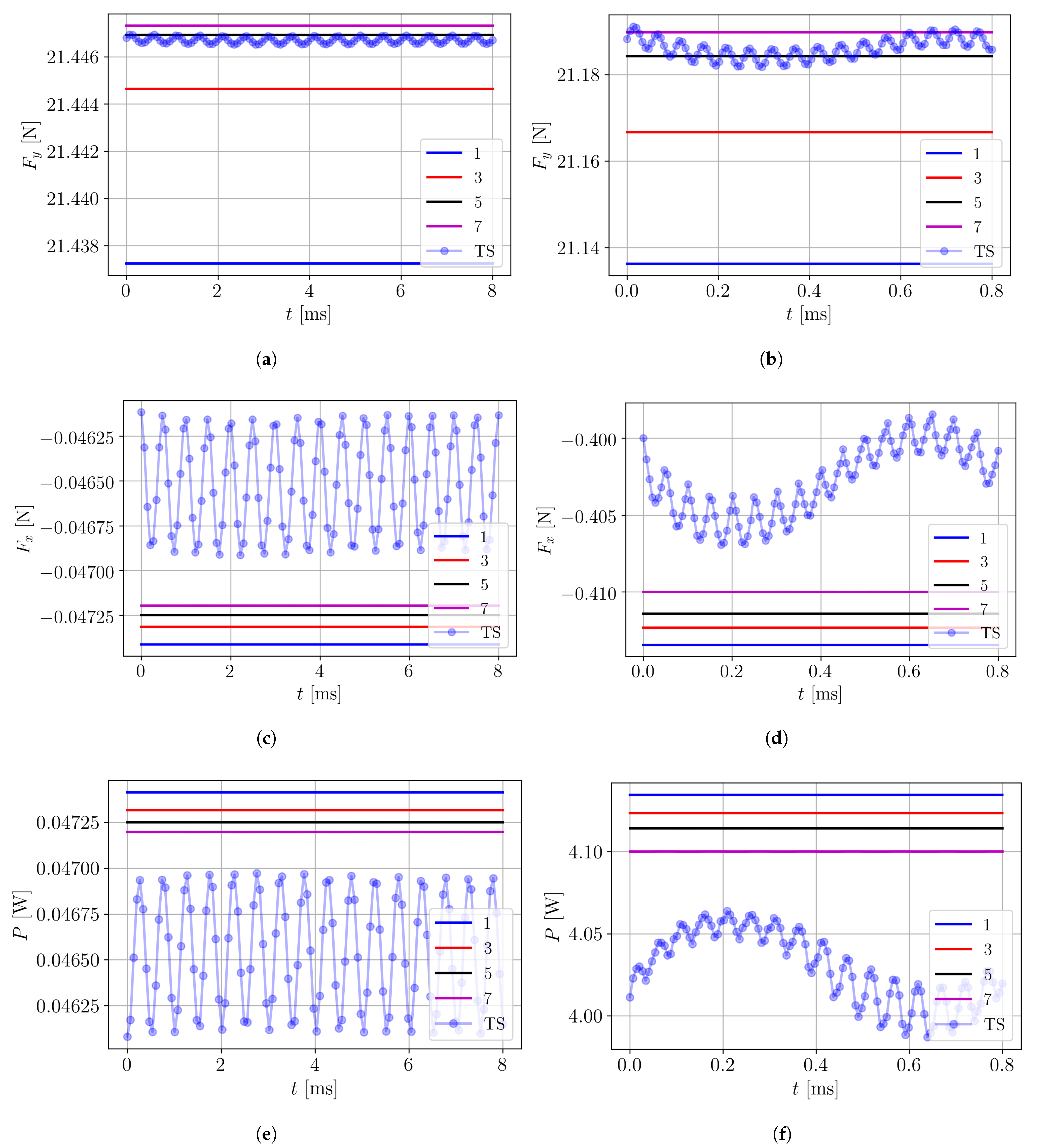
3.3. Comparison with the Space-Time Approach
3.4. Refinement Strategy
4. Conclusions
Funding
Acknowledgments
Conflicts of Interest
Abbreviations
| 1D, 2D, 3D, 4D | One-, Two-, Three-, Four-dimensional |
| 2.5D | Two and a half dimensional |
| BE | Backward Euler |
| B-spline | Basis spline |
| CAD | Computer-Aided Design |
| CG | Continuous Galerkin |
| CK | Crank–Nicolson |
| DC | Direct Current |
| dofs | degrees of freedom |
| DCT | Discrete Cosine Transform |
| DFT | Discrete Fourier Transform |
| DG | Discontinuous Galerkin |
| FEM | Finite Element Method |
| FE | Forward Euler |
| FPM | Fixed-Point Method |
| GAMG | Geometric Algebraic Multigrid |
| GMG | Geometric Multigrid |
| GMRES | Generalized Minimal Residual |
| HB | Harmonic Balance |
| IGA | Isogeometric Analysis |
| LF | Leapfrog |
| MEMS | Microelectromechanical Systems |
| MG | Multigrid |
| NRM | Newton–Raphson Method |
| NURBS | Non-Uniform Rational B-splines |
| PDEs | Partial Differential Equations |
| QMR | Quasi-Minimal Residual |
| RF | Radio Frequency |
| rms | Root Mean Square |
| ST | Space-Time |
| THB-spline | Truncated Hierarchical B-spline |
| THD | Total Harmonic Distortion |
| TP | Time-Periodic |
| TS | Time-Stepping |
References
- Quarteroni, A.; Quarteroni, S. Numerical Models for Differential Problems; Springer: Milan, Italy, 2009. [Google Scholar]
- Loli, G.; Montardini, M.; Sangalli, G.; Tani, M. Space-time Galerkin isogeometric method and efficient solver for parabolic problem. arXiv preprint 2019, arXiv:1909.07309. [Google Scholar] [CrossRef]
- Hofer, C.; Langer, U.; Neumüller, M.; Toulopoulos, I. Time-multipatch discontinuous Galerkin space-time isogeometric analysis of parabolic evolution problems. Verlag Österreichischen Akademie Wissenschaften 2018. [Google Scholar] [CrossRef]
- Yamada, S.; Bessho, K.; Lu, J. Harmonic balance finite element method applied to nonlinear AC magnetic analysis. IEEE Trans. Magn. 1989, 25, 2971–2973. [Google Scholar] [CrossRef]
- Yamada, S.; Biringer, P.; Bessho, K. Calculation of nonlinear eddy-current problems by the harmonic balance finite element method. IEEE Trans. Magn. 1991, 27, 4122–4125. [Google Scholar] [CrossRef]
- De Gersem, H.; Gyselinck, J.; Dular, P.; Hameyer, K.; Weiland, T. Comparison of sliding-surface and moving-band techniques in frequency-domain finite-element models of rotating machines. COMPEL Int. J. Comput. Math. Electr. Electron. Eng. 2004. [Google Scholar] [CrossRef]
- Demenko, A.; Hameyer, K.; Nowak, L.; Zawirski, K.; De Gersem, H.; Ion, M.; Wilke, M.; Weiland, T. Trigonometric interpolation at sliding surfaces and in moving bands of electrical machine models. COMPEL- Int. J. Comput. Math. Electr. Electron. Eng. 2006. [Google Scholar] [CrossRef]
- Hughes, T.J.R.; Cottrell, J.A.; Bazilevs, Y. Isogeometric analysis: CAD, finite elements, NURBS, exact geometry and mesh refinement. Comput. Methods Appl. Mech. Eng. 2005, 194, 4135–4195. [Google Scholar] [CrossRef]
- De Boor, C. A Practical Guide to Splines; Applied Mathematical Sciences; Springer: New York, NY, USA, 1978; Volume 27. [Google Scholar]
- Friedrich, L.A.J.; Roes, M.G.L.; Gysen, B.L.J.; Lomonova, E.A. Adaptive isogeometric analysis applied to an electromagnetic actuator. IEEE Trans. Magn. 2019, 55, 1–4. [Google Scholar] [CrossRef]
- Farin, G.; Hansford, D. Discrete Coons patches. Comput. Aided Geom. Des. 1999, 16, 691–700. [Google Scholar] [CrossRef]
- Hinz, J.; Möller, M.; Vuik, C. Elliptic grid generation techniques in the framework of isogeometric analysis applications. Comput. Aided Geom. Des. 2018, 65, 48–75. [Google Scholar] [CrossRef]
- Hinz, J.; Abdelmalik, M.; Möller, M. Goal-Oriented Adaptive THB-Spline Schemes for PDE-Based Planar Parameterization. arXiv 2020, arXiv:2001.08874. [Google Scholar]
- Buffa, A.; Corno, J.; de Falco, C.; Schöps, S.; Vázquez, R. Isogeometric Mortar Coupling for Electromagnetic Problems. SIAM J. Sci. Comput. 2020, 42, B80–B104. [Google Scholar] [CrossRef]
- Buffa, A.; Perugia, I. Discontinuous Galerkin approximation of the Maxwell eigenproblem. SIAM J. Numer. Anal. 2006, 44, 2198–2226. [Google Scholar] [CrossRef]
- Piegl, L.; Tiller, W. The NURBS Book; Springer Science & Business Media: Berlin/Heidelberg, Germany, 2012. [Google Scholar]
- Vázquez, R. A new design for the implementation of isogeometric analysis in Octave and Matlab: GeoPDEs 3.0. Comput. Math. Appl. 2016, 72, 523–554. [Google Scholar] [CrossRef]
- Friedrich, L.A.J.; Curti, M.; Gysen, B.L.J.; Lomonova, E.A. High-order methods applied to nonlinear magnetostatic problems. Math. Comput. Appl. 2019, 24, 19. [Google Scholar] [CrossRef]
- Ramière, I.; Helfer, T. Iterative residual-based vector methods to accelerate fixed point iterations. Comput. Math. Appl. 2015, 70, 2210–2226. [Google Scholar] [CrossRef]
- Kuzmin, D. A Guide to Numerical Methods for Transport Equations; University Erlangen-Nuremberg: Erlangen, Germany, 2010. [Google Scholar]
- Gödel, N.; Schomann, S.; Warburton, T.; Clemens, M. GPU accelerated Adams–Bashforth multirate discontinuous Galerkin FEM simulation of high-frequency electromagnetic fields. IEEE Trans. Magn. 2010, 46, 2735–2738. [Google Scholar] [CrossRef]
- Palha, A.; Koren, B.; Felici, F. A mimetic spectral element solver for the Grad–Shafranov equation. J. Comput. Phys. 2016, 316, 63–93. [Google Scholar] [CrossRef]
- Agilent Technologies. Advanced Design System. In Harmonic Balance Simulation, User Guide; 2011. [Google Scholar]
- Cvijetić, G.; Gatin, I.; Vukčević, V.; Jasak, H. Harmonic Balance developments in OpenFOAM. Comput. Fluids 2018, 172, 632–643. [Google Scholar] [CrossRef]
- Weeger, O.; Wever, U.; Simeon, B. Isogeometric analysis of nonlinear Euler–Bernoulli beam vibrations. Nonlinear Dyn. 2013, 72, 813–835. [Google Scholar] [CrossRef]
- Plasser, R.; Koczka, G.; Bíró, O. A nonlinear magnetic circuit model for periodic eddy current problems using T,Φ-Φ formulation. COMPEL- Int. J. Comput. Math. Electr. Electron. Eng. 2017. [Google Scholar] [CrossRef]
- Plasser, R.; Takahashi, Y.; Koczka, G.; Bíró, O. Comparison of two methods for the finite element steady-state analysis of nonlinear 3D periodic eddy-current problems using the A,V-formulation. Int. J. Numer. Model. Electron. Netw. Devices Fields 2018, 31, e2279. [Google Scholar] [CrossRef]
- Plasser, R.; Koczka, G.; Bíró, O. Improvement of the Finite-Element Analysis of 3D, Nonlinear, Periodic Eddy Current Problems Involving Voltage-Driven Coils under DC Bias. IEEE Trans. Magn. 2017, 54, 1–4. [Google Scholar] [CrossRef]
- Zhao, X.; Guan, D.; Meng, F.; Zhong, Y.; Cheng, Z. Computation and Analysis of the DC-Biasing Magnetic Field by the Harmonic-Balanced Finite-Element Method. Int. J. Energy Power Eng. 2015, 5, 31. [Google Scholar] [CrossRef][Green Version]
- Bachinger, F.; Langer, U.; Schöberl, J. Efficient solvers for nonlinear time-periodic eddy current problems. Comput. Vis. Sci. 2006, 9, 197–207. [Google Scholar] [CrossRef][Green Version]
- Hollaus, K. A MSFEM to simulate the eddy current problem in laminated iron cores in 3D. COMPEL Int. J. Comput. Math. Electr. Electron. Eng. 2019, 38, 1667–1682. [Google Scholar] [CrossRef]
- Roppert, K.; Toth, F.; Kaltenbacher, M. Simulating induction heating processes using harmonic balance FEM. COMPEL Int. J. Comput. Math. Electr. Electron. Eng. 2019, 38, 1562–1574. [Google Scholar] [CrossRef]
- Halbach, A.; Geuzaine, C. Steady-state, nonlinear analysis of large arrays of electrically actuated micromembranes vibrating in a fluid. Eng. Comput. 2018, 34, 591–602. [Google Scholar] [CrossRef]
- Pries, J.; Hofmann, H. Harmonic balance FEA of synchronous machines using a traveling-wave airgap model. In Proceedings of the 2011 IEEE Vehicle Power and Propulsion Conference, Chicago, IL, USA, 6–9 September 2011; pp. 1–6. [Google Scholar]
- Wick, M.; Grabmaier, S.; Juettner, M.; Rucker, W. Motion in frequency domain for harmonic balance simulation of electrical machines. COMPEL- Int. J. Comput. Math. Electr. Electron. Eng. 2018, 37, 1449–1460. [Google Scholar] [CrossRef]
- Driesen, J.; Van Craenenbroeck, G.D.T.; Hameyer, K. Implementation of the harmonic balance FEM method for large-scale saturated electromagnetic devices. WIT Trans. Eng. Sci. 1999, 22, 10. [Google Scholar]
- Friedrich, L.A.J.; Gysen, B.L.J.; Lomonova, E.A. Modeling of integrated eddy current damping rings for a tubular electromagnetic suspension system. In Proceedings of the 12th International Symposium on Linear Drives for Industry Applications (LDIA), Neuchâtel, Switzerland, 1–3 July 2019; pp. 1–4. [Google Scholar]
- De Gersem, H.; Vande Sande, H.; Hameyer, K. Strong coupled multi-harmonic finite element simulation package. COMPEL Int. J. Comput. Math. Electr. Electron. Eng. 2001, 20, 535–546. [Google Scholar] [CrossRef]
- Bachinger, F. Multigrid Solvers for 3D Multiharmonic Nonlinear Magnetic Field Computations. Ph.D. Thesis, Johannes Kepler Universitat Linz, 2003. [Google Scholar]
- Friedrich, L.A.J.; Gysen, B.L.J.; Jansen, J.W.; Lomonova, E.A. Analysis of Motional Eddy Currents in the Slitted Stator Core of an Axial-Flux Permanent-Magnet Machine. IEEE Trans. Magn. 2020, 56, 1–4. [Google Scholar] [CrossRef]
- Saad, Y. Iterative Methods for Sparse Linear Systems; SIAM: Philadelphia, PA, USA, 2003. [Google Scholar]
- Pries, J.; Hofmann, H. Steady-state algorithms for nonlinear time-periodic magnetic diffusion problems using diagonally implicit Runge–Kutta methods. IEEE Trans. Magn. 2014, 51, 1–12. [Google Scholar] [CrossRef]
- Reitzinger, S.; Schöberl, J. An algebraic multigrid method for finite element discretizations with edge elements. Numer. Linear Algebra Appl. 2002, 9, 223–238. [Google Scholar] [CrossRef]
- OpenCFD Ltd. OpenFOAM: API Guide. Available online: www.openfoam.com (accessed on 7 January 2021).
- Tielen, R.; Möller, M.; Göddeke, D.; Vuik, C. Efficient p-multigrid methods for isogeometric analysis. arXiv 2019, arXiv:1901.01685. [Google Scholar]
- de Prenter, F.; Verhoosel, C.V.; van Brummelen, E.H.; Evans, J.A.; Messe, C.; Benzaken, J.; Maute, K. Scalable multigrid methods for immersed finite element methods and immersed isogeometric analysis. arXiv 2019, arXiv:1903.10977. [Google Scholar]
- Außerhofer, S.; Bíró, O.; Preis, K. An efficient harmonic balance method for nonlinear eddy-current problems. IEEE Trans. Magn. 2007, 43, 1229–1232. [Google Scholar] [CrossRef]
- Flux 12.2, User’s Guide and Material Library; 2016.
- van Zwieten, G.; van Zwieten, J.; Verhoosel, C.V.; Fonn, E.; van Opstal, T.; Hoitinga, W. Nutils (Version 7.0). Available online: www.nutils.org (accessed on 7 January 2021).


| Name | Scheme | Precision | |
|---|---|---|---|
| 0 | Forward Euler | explicit | |
| 0.5 | Crank–Nicolson | implicit | |
| 1 | Backward Euler | implicit |
| Parameter | Value [mm] | Parameter | Value [mm] |
|---|---|---|---|
| 8.0 | 10.5 | ||
| 2.0 | 2.0 | ||
| g | 1.0 | 1.5 | |
| 2.0 | 1.5 | ||
| 2.0 | 2.0 |
| [%] | [%] | [%] | |||||
|---|---|---|---|---|---|---|---|
| 1 m/s | 10 m/s | 1 m/s | 10 m/s | 1 m/s | 10 m/s | ||
| 1 | 1 | 4.41 × | 2.36 × 10 | ||||
| 2 | 3 | 9.63 × 10 | 9.20 × 10 | ||||
| 3 | 5 | 1.54 × 10 | 1.04 × 10 | 8.81 × 10 | |||
| 4 | 7 | 1.43 × 10 | 2.84 × 10 | 1.73 × 10 | |||
| [%] | [%] | [%] | |||||
|---|---|---|---|---|---|---|---|
| mean | rms | mean | rms | mean | rms | ||
| 1 | 1 | ||||||
| 2 | 3 | ||||||
| 3 | 5 | ||||||
| 4 | 7 | ||||||
| 5 | 9 | ||||||
| Slotless | Slotted | |||||
|---|---|---|---|---|---|---|
| HB(2) | ST | TS | HB(4) | ST | TS | |
| Time [s] | 24 | 119 | 821 | 138 | 236 | 1470 |
| Ratio [-] | - | 5.0 | 34.4 | - | 1.72 | 10.6 |
Publisher’s Note: MDPI stays neutral with regard to jurisdictional claims in published maps and institutional affiliations. |
© 2021 by the author. Licensee MDPI, Basel, Switzerland. This article is an open access article distributed under the terms and conditions of the Creative Commons Attribution (CC BY) license (http://creativecommons.org/licenses/by/4.0/).
Share and Cite
Friedrich, L.A.J. Time- and Frequency-Domain Steady-State Solutions of Nonlinear Motional Eddy Currents Problems. J 2021, 4, 22-48. https://doi.org/10.3390/j4010002
Friedrich LAJ. Time- and Frequency-Domain Steady-State Solutions of Nonlinear Motional Eddy Currents Problems. J. 2021; 4(1):22-48. https://doi.org/10.3390/j4010002
Chicago/Turabian StyleFriedrich, Léo A.J. 2021. "Time- and Frequency-Domain Steady-State Solutions of Nonlinear Motional Eddy Currents Problems" J 4, no. 1: 22-48. https://doi.org/10.3390/j4010002
APA StyleFriedrich, L. A. J. (2021). Time- and Frequency-Domain Steady-State Solutions of Nonlinear Motional Eddy Currents Problems. J, 4(1), 22-48. https://doi.org/10.3390/j4010002