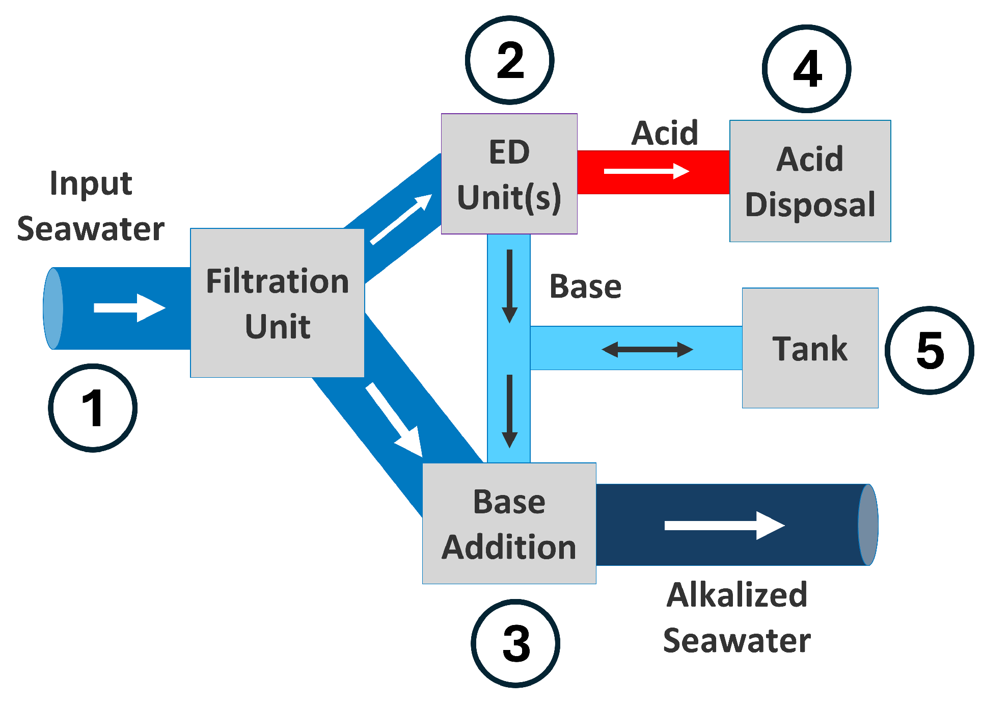
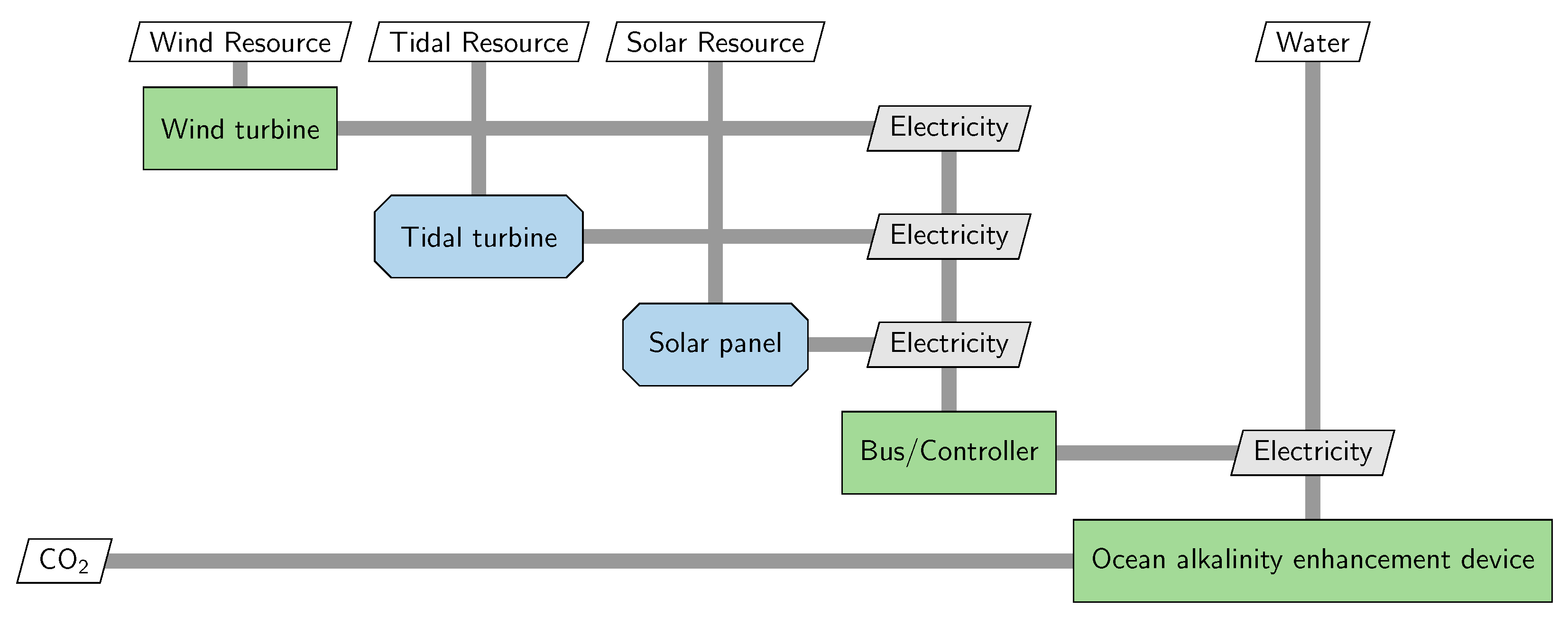
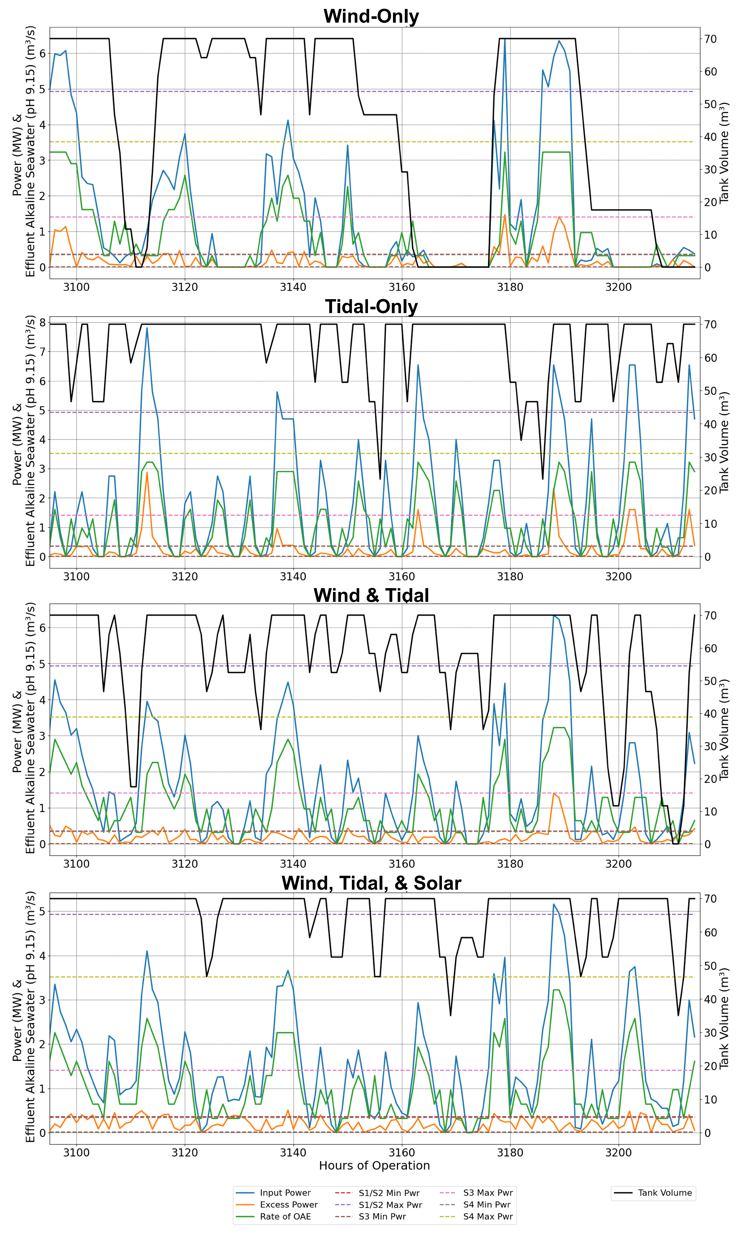
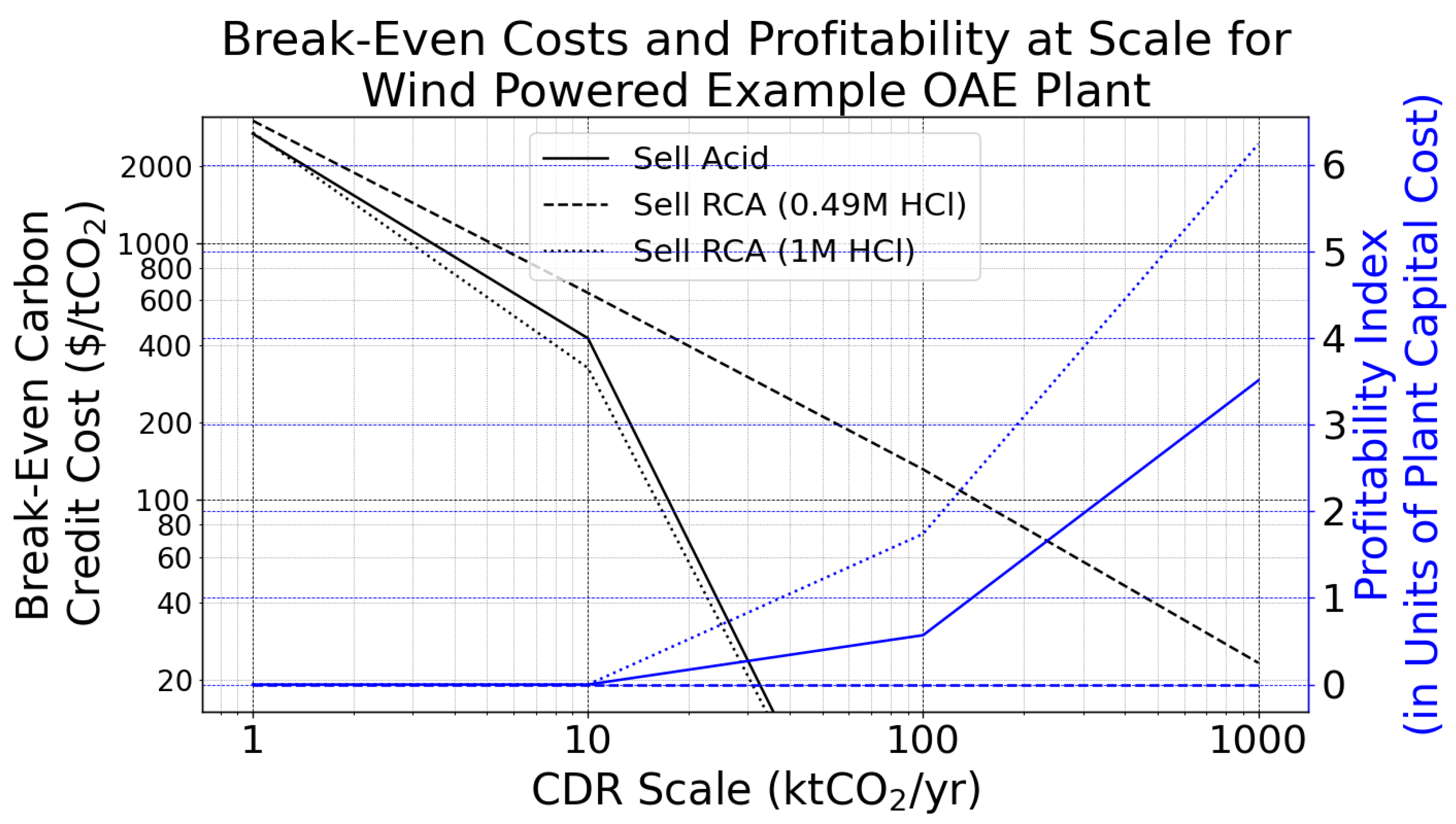
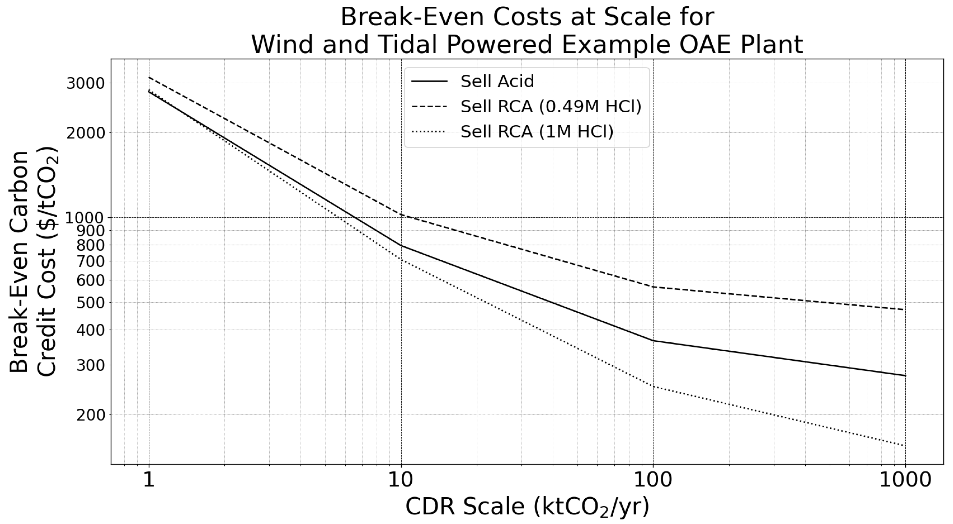
This study focuses on evaluating a theoretical developmental-level 10 ktCO
2/yr scale electrochemical OAE plant, assumed to be connected to an existing theoretical desalination plant and therefore uses input brine rather than seawater. The parameters of the modeled example plant are shown in
Table 1. Note that
is the maximum amount of active ED units,
and
are the maximum power need and flow rate for the ED system,
is the fraction of ED flow that becomes base,
and
are the concentrations of the generated acid and base,
is the ratio of ED flow to intake flow,
and
are the pH and temperature of the intake brine/seawater,
and
are the concentrations of dissolved inorganic carbon (DIC) and salinity of the intake brine/seawater,
and
are the temperature increases from the ED and desalination systems,
is the weight fraction of CaO in RCA,
is the fraction of CaO that dissolves from the RCA,
is the power need to mix the RCA and acid,
is the fraction of RCA that can be sold,
d is the days of the simulation,
is the pump efficiency, the
inputs refer to the pressure drop ranges of the active pumps, and
is the hours of minimum OAE enabled by tank storage.
Most of the parameters used in this model were based on those used in literature [
9,
10,
11,
20,
21]. Many of the OAE plant inputs were adapted from Ferella et al. [
9] who assessed a roughly 1 ktCO
2/yr scale system connected to a desalination plant. The
and
values from their work were scaled up by a factor of 10 for the analysis of the case study plant, while their values for
,
,
, and
were directly used and their pump inputs were estimated, see
Section 2.9 for more details on the literature parameters used [
9]. Their cost inputs were also scaled using a learning rate method, see
Section 2.6. Meanwhile, the values for
,
, and
were based on feedback from our industry partner.
The overall model was validated both by comparing the results for a 1 ktCO
2/yr scale plant with inputs from Ferella et al. [
9] and a 8 ktCO
2/yr scale plant with inputs from our industry partner (see
Section 2.9). Additionally, the operational scenarios were confirmed to function appropriately by examining the plant performance under an example sine wave power profile, which was also used to compare plant performance between selling acid and RCA (
Section 2.10.1). The break-even carbon credit costs and performance of the developmental-level plant were then assessed under the two acid disposal options with microgrids containing different energy sources, as described in
Section 2.10.2. The two microgrid configurations that resulted in the lowest break-even carbon credit costs were used to evaluate the plant at varying scales from developmental (1 to 10 ktCO
2/yr) to commercial (100 to 1000 ktCO
2/yr) to determine if revenue from the co-products could remove the need for carbon credits at commercial scales (
Section 2.10.3) [
3,
4,
5,
6].
2.1. Electrochemistry Model
As described in
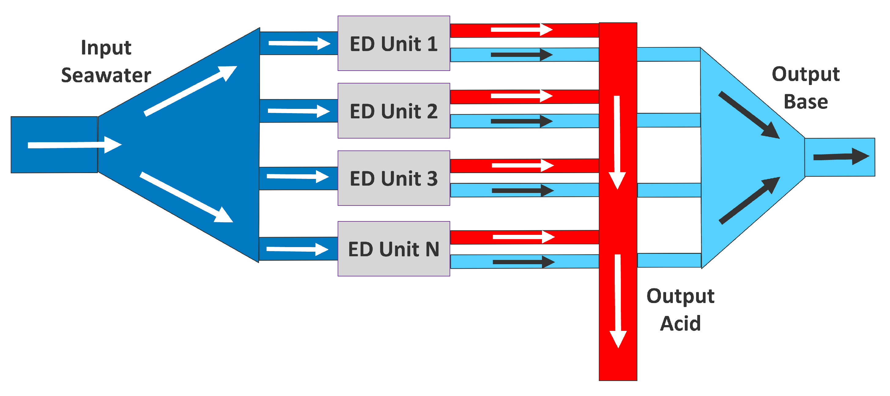
Section 2, the ability of the ED system to use variable power is accounted for by splitting it into individual “units,” each with the same power, intake flow rate, output flow rates of acid and base, and concentrations of acid and base (
Figure 4) [
11]. In contrast to the previous work on the direct ocean capture model (which determined acid and base concentrations based on user ED efficiencies), the concentrations of acid and base are user inputs for the OAE model, as these values are more commonly reported and known by developers than ED efficiencies. However, the efficiencies of the ED system at producing acid and base (
and
in Wh/mol HCl and Wh/mol NaOH, respectively) are still reported and determined using the equations below [
11,
22]:
where
is the maximum power needed by the ED system in watts,
and
are the maximum output flow rates of the acid and base in m
3/s,
and
are the concentrations of acid and base produced in mol/m
3,
is the input flow rate to the ED system in m
3/s, and
and
are the concentrations of acid and base in the input seawater in mol/m
3.
and
are direct inputs for the model while
and
are found by converting the input concentrations from mol/L to mol/m
3.
and
are found using the pH of seawater,
, which is typically around 8.1, and the water dissociation constant,
, which is determined using the same equation as in our previous direct ocean capture work [
11]:
Unlike the previous direct ocean capture model, the flow rates of acid and base are not assumed to be equal to each other; instead, a fraction of base flow (
) is used as a user input to determine the flow rates of acid and base [
11]:
The power needs of the ED system (
), the flow rates into the ED system (
), and the output flow rates of acid and base (
and
) vary linearly with the number of active ED units,
, but the concentrations of acid and base remain the same [
11]. The minimum amount of active ED units,
, is 1 as a default, and
is the flow rate needed for one ED unit:
The overall intake of seawater for the OAE plant is determined by the number of active ED units since the ED flow rate is a fraction,
, of the intake flow rate
. By default the model assumes that 1% of the intake flow rate is used by the ED system, meaning that the intake flow rate is 100 times larger than the flow rate of the ED system, as was done in our prior direct ocean capture work and confirmed as reasonable by our OAE industry partner for this work [
11]:
The input parameters for this model are shown in
Table 1.
2.2. Ocean Chemistry Model
Unlike previous work, the seawater chemistry is not approximated as a carbonate buffer solution but instead utilizes PyCO2SYS (Version v2.0.0-b5), a Python toolbox that can account for additional chemical species in the marine carbonate system and calculate seawater characteristics such as pH and total alkalinity (TA) [
11,
23,
24]. The ocean chemistry model relies on inputs for the initial DIC concentration, pH, ambient temperature, and salinity. Additionally, this part of the model accounts for the slight temperature increases that the ED system can have on the seawater,
, which is 2 °C by default per feedback from our industry partner.
In this case, our team was interested in modeling how the system could be co-located with a desalination plant to utilize the effluent brine of the plant in place of seawater, which could minimize costs [
9,
25]. Therefore, the salinity input,
, and DIC input,
, were higher than usual for seawater (
Table 1). Additionally, the desalination process can increase the temperature of the brine,
, which by default is also assumed to be roughly 2 °C. This model is generalizable, so if a user prefers to use saltwater inputs, the temperature increase can be set to zero (
Table 1). Inputs to PyCO2SYS included pH, salinity, temperature, and concentrations of TA, DIC, and calcium, while other parameters were left at their default values [
23,
24]. Additionally the default methods for the equilibrium constant parameterization [
26] and total pH scale [
27] were used. See
Section 2.7 for details on the assumptions made when using PyCO2SYS.
Base Addition
The resulting pH after the base addition in the third step of
Figure 3 is determined by first finding the TA, salinity, and temperature of the mixed base and seawater solutions. The new values of TA and salinity in mol/m
3 (
and
) were found by comparing the sum of moles divided by the change in volume or, in this case, the flow rate, as described in the following equations, where
is the initial salinity
converted from ppt to mol/m
3:
The salinity in the base stream is lower than that of the brine/seawater stream since a portion of the salinity was consumed to create the higher concentration of base. Because of this, the model also alerts the user if the concentration of base or acid is higher than that of the salinity. Simply put:
and
. Additionally, since the brine/seawater is considered to have the same specific heat and density, the temperature of the mixed solutions,
, can be found using the same formulation as that of the TA and salinity while accounting for the changes in temperature from the desalination system and the ED system:
After the TA, salinity, and temperature values of the mixed solution are determined they are used as inputs along with the DIC, which does not change since both solutions have the same DIC concentrations, into PyCO2SYS to determine the pH of the solution. Other inputs for PyCO2SYS are set to default conditions. The equations described in this section are specifically for the case where the acid is sold; see
Section 2.3.1 for details on how the TA, salinity, and temperature are impacted by using RCA for acid disposal.
2.5. Operational Scenarios
Including chemical storage tanks enables the model to apply a heuristic operational strategy to evaluate how the plant could operate under variable power availability, similar to what was done in our previous direct ocean capture plant model [
11]. As described in
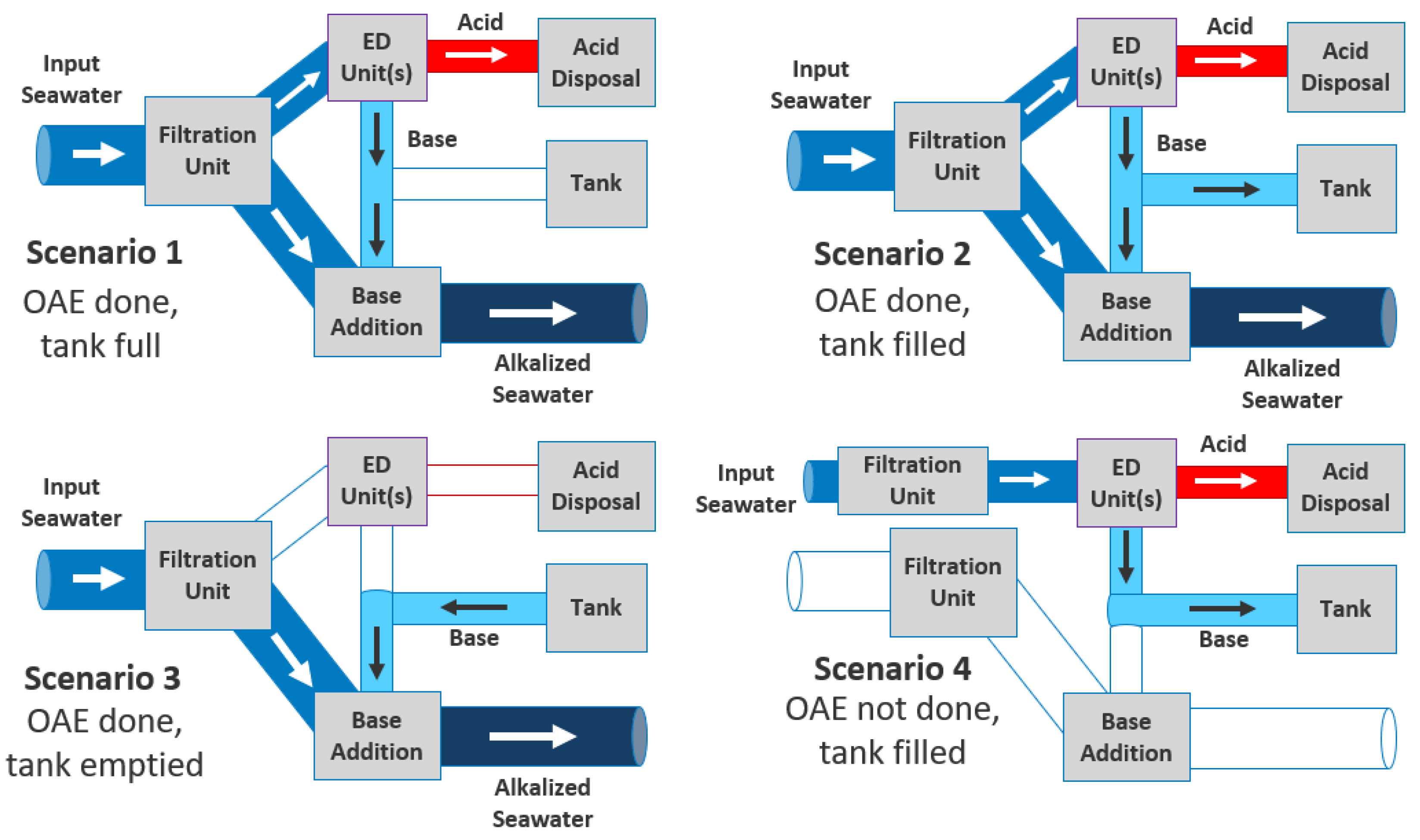
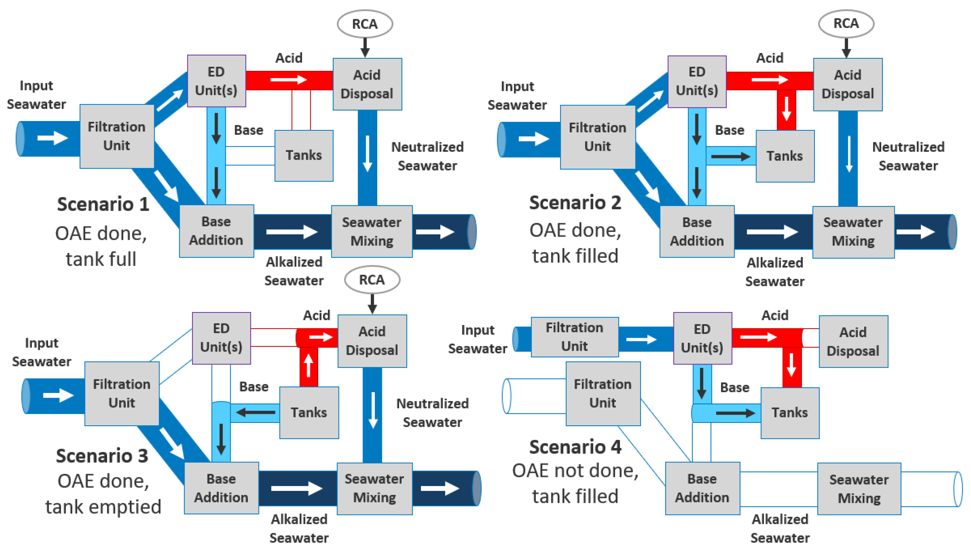
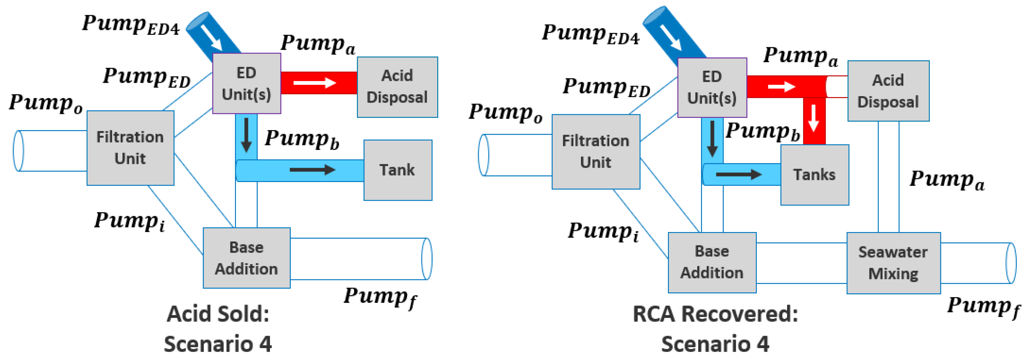
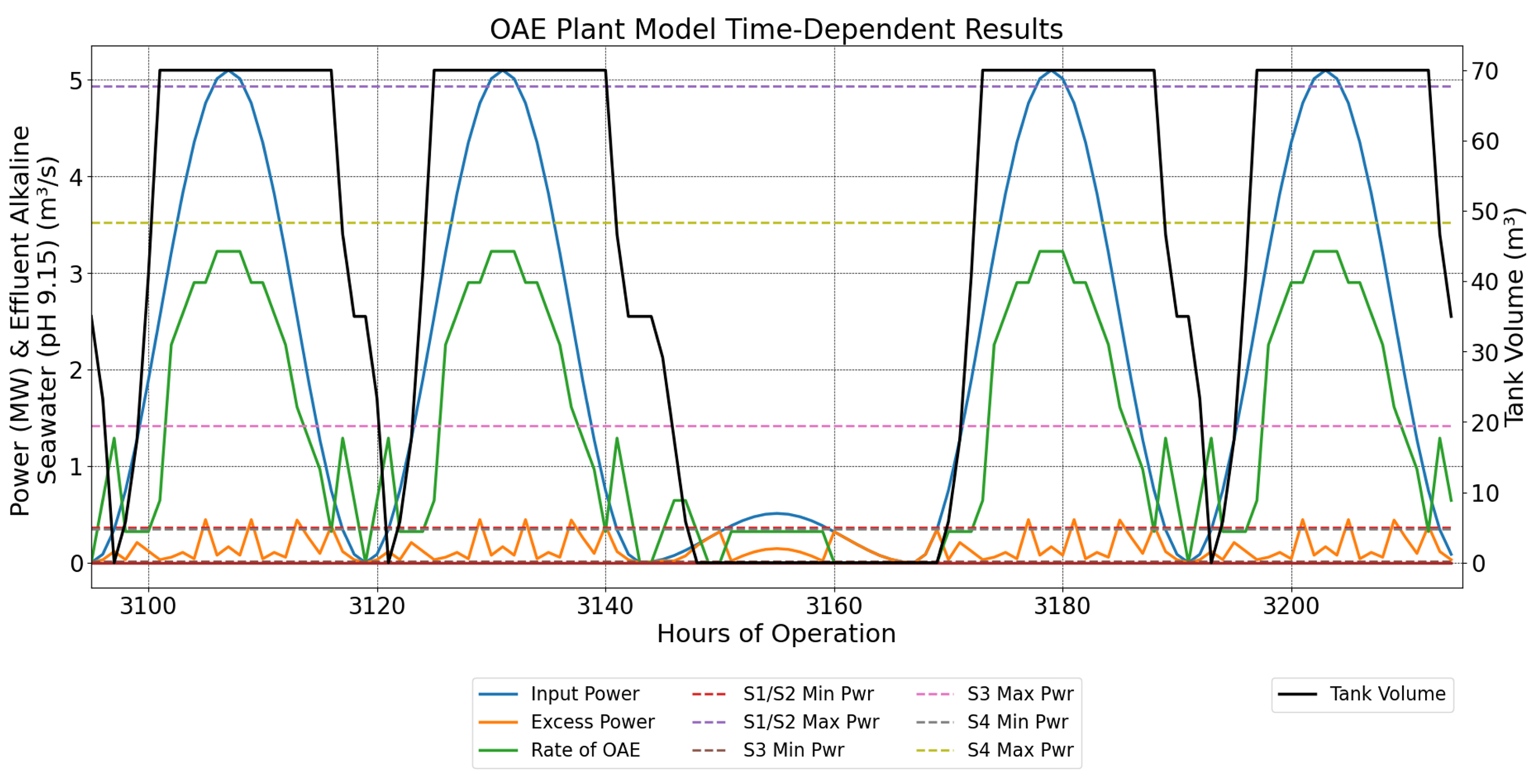
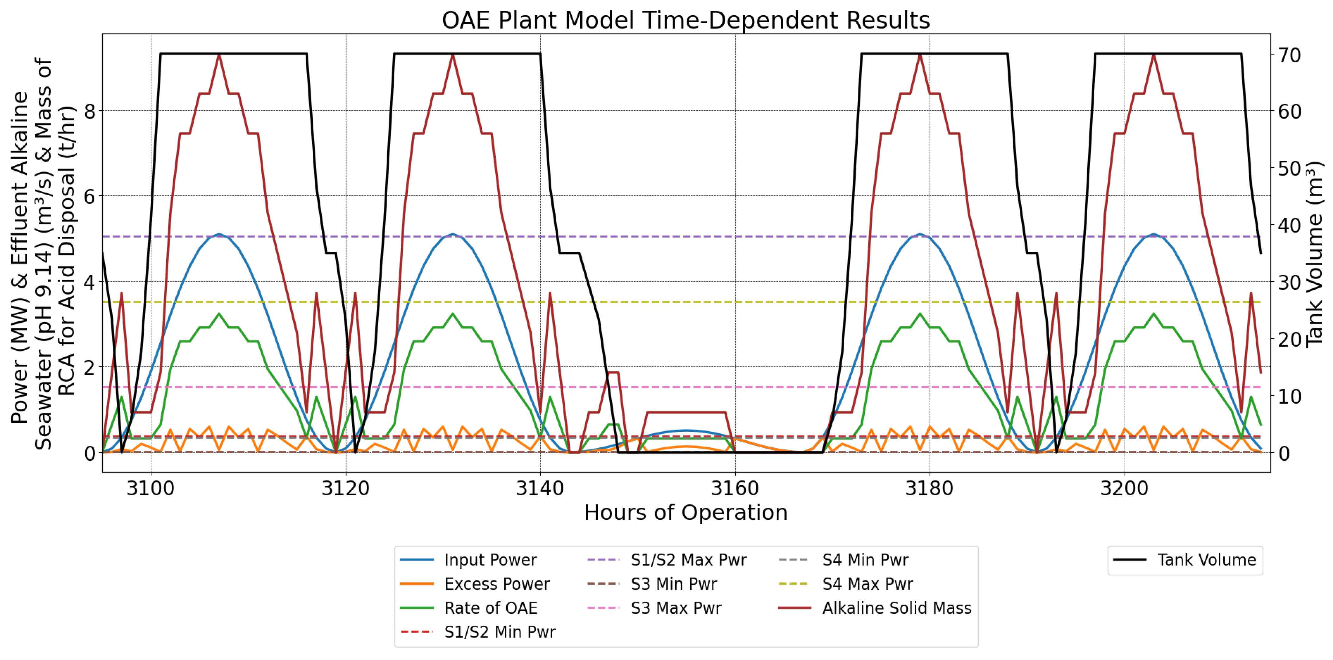
Section 2, there are four primary operational scenarios. If RCA is used for acid disposal, then whenever OAE is done, so is the acid disposal, meaning that the acid is also stored in a separate tank when RCA is processed on-site. In Scenario 1 the tank is full, so the base generated by the ED system is used for OAE while the acid is disposed of. This can also be approximated to typical operation without considering chemical storage. In Scenario 2, there is enough energy to enable OAE but the tanks are not full; therefore, a portion of the chemical solutions generated during the time step is stored in the tanks while the rest is used for OAE. In Scenario 3, there is not enough power available to activate the ED system but there is enough to pump base from the tanks for OAE, and acid for disposal. Scenario 4 is triggered only when there is not enough base in the tanks for OAE to be done via Scenario 3, but there is just enough power to activate the ED system to fill the tanks. See
Figure 5 and
Figure 6 for what these operational scenarios look like for selling the acid and using it to recover RCA. Finally, Scenario 5 occurs when there is not enough power or volume to activate the other scenarios. If the modeled microgrid has a battery system then this power can be stored for later use, otherwise the power is excess.
The input and output ranges for each operational scenario (power needs, moles of NaOH added to the seawater, and effluent flow rate and chemistry) are initialized prior to simulating the plant’s performance at each time step. They are then referenced during the time-dependent analysis given the amount of power and tank volume available. These ranges are based on the number of active ED units, or equivalent for Scenario 3. The total number of cases within Scenarios 1, 3, and 4,
, is therefore:
The example OAE plant has a maximum number of 10 ED units and by default has a minimum of 1 ED unit, meaning
is 10 (
Table 1). The specific hourly output values depend on the number of units or equivalent that can be activated at the hourly time step,
. For scenarios 1, 3, and 4 all of the ED units are used to either solely conduct OAE and acid disposal or solely fill the tanks. However, in Scenario 2 there are more output values since the number of units conducting OAE,
, versus filling the tanks,
, can vary. In this scenario, filling the tank or tanks is prioritized while at least one ED unit is used for OAE and acid disposal. See our prior direct ocean capture model work for more details on how the output values from Scenario 2 are calculated and selected during the time-dependent analysis [
11]. The overall power needs for each of these output cases depend on the number of ED units powered, flow rates into and out of the system, and the rotary drum if RCA is being recovered.
The default maximum volume of the base (
) and acid when RCA is being recovered (
), depend on the total storage time (
) and the flow rates of base and acid provided by the minimum number of ED units:
These volumes were selected to enable the tanks to facilitate conducting the minimum OAE rate over the duration of the storage time, which is set to 12 h for the example plant [
11].
To clarify the flow rates of acid and base sent to the tanks compared to those used for acid disposal and OAE they are labeled as
,
,
, and
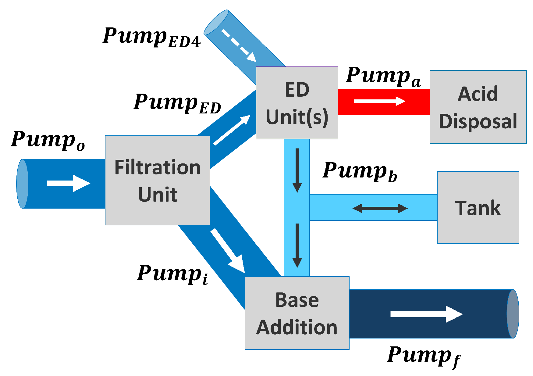
, respectively. These flow rates are enabled by the acid and base pumps such that
and
, except for in Scenario 3 where the solutions are pumped from the tanks, are
and
. Note that
is only nonzero if the RCA method is used for acid disposal. Additionally,
and
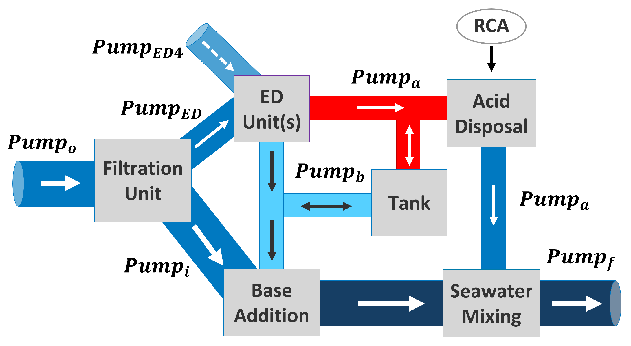
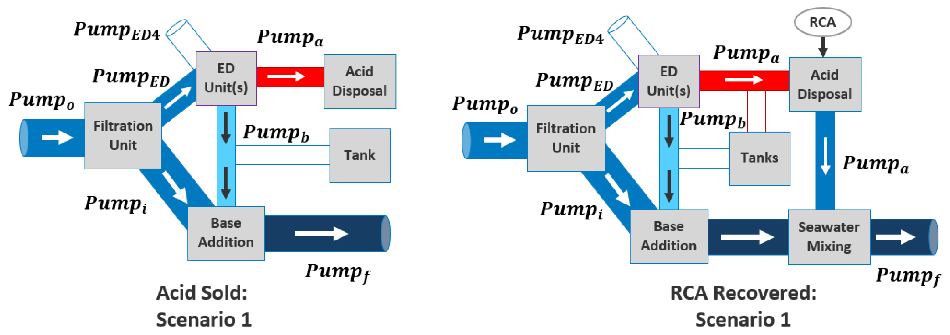
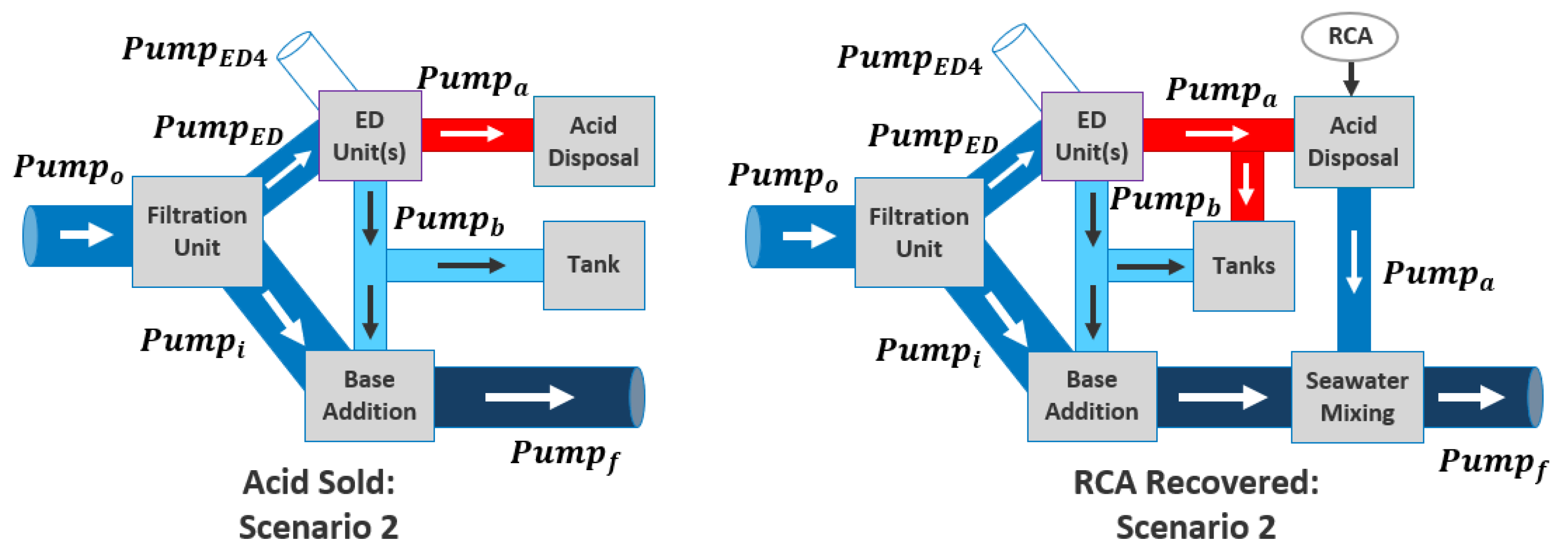
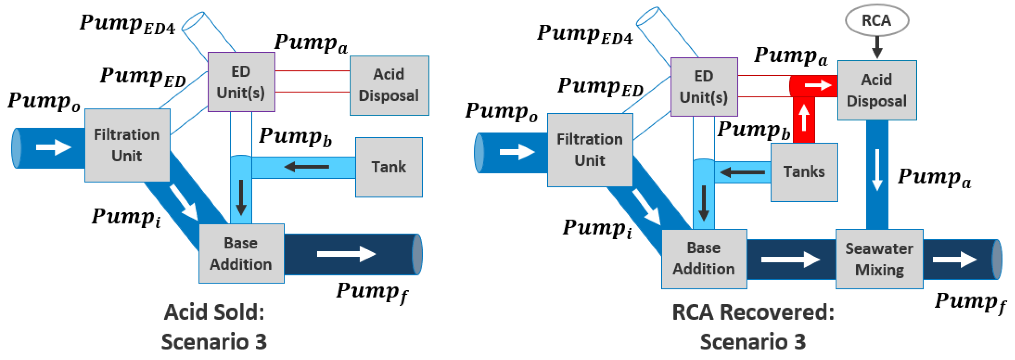
must be nonzero if any acid and base are flowing since pumps “a” and “b” enable these flow rates. The pumps and flow rates used for each of the four primary scenarios under direct acid disposal and using RCA are shown in
Figure 9,
Figure 10,
Figure 11 and
Figure 12 and
Table 2,
Table 3,
Table 4,
Table 5,
Table 6,
Table 7,
Table 8 and
Table 9.
2.6. Cost Model
The cost model adapts and modifies the methodology used by Ferella et al. [
9] who conducted an in-depth cost analysis on a theoretical 1 ktCO
2/yr developmental-level scale ED-based OAE plant connected to a desalination plant. The team also accounted for potential revenue from selling the dilute acid, which can be used to reduce the cost of carbon credits needed for the electrochemical OAE plant to break even or recover their investment (
) [
9]. Though the analysis by Ferella et al. [
9] was done in Excel, the equations and methodology were adapted into Python to run with the rest of our models. Since the cost model is largely based on prior literature, its methodology is described in more detail in our supplementary cost model description.
A few alterations were made to the methodology used by Ferella et al. [
9]. First, we included an automatic adjustment feature that can simplify user inputs by applying a learning rate to account for how costs can be impacted by plant scales. Next, we incorporated cost estimates for the acid disposal option to recover RCA on-site [
10]. Additionally, the net present value (NPV) calculation used by Ferella et al. [
9] included accounting for negative tax values, which in this model has been adjusted to account for earnings before interest, taxes, depreciation, and amortization (EBITA) and carried-forward tax losses. Note that the carried-forward tax losses are only nonzero while the yearly taxable income is less than the tax losses of the prior year, which can occur in the first few years of a plant’s life, see
Section S5 of the supplementary cost model document for more details. Finally, our analysis focuses on determining the cost of carbon credits necessary for a plant to break even or recover their investment, resulting in a profitability index (PI) of zero. Ferella et al. [
9] were interested in carbon credit values that would enable their plant to have a PI of 1.03 or earn a profit equivalent to 103% of their capital cost. Our model can report nonzero PIs but only when the revenue from co-products like dilute acid or RCA make carbon credits unnecessary for a plant to break even.
Inputs to the cost model are either direct or from the other models. Inputs from the OAE plant model include the mass and value of sold materials like the acid or RCA recovered, the amount of NaOH added to the ocean, and the maximum estimated CDR capacity. Additionally the model receives the yearly cost of energy from the hybrid energy models from H2I, (
Section 2.8).
The cost model has a maximum of 27 possible direct user inputs, including the capital costs of the ED system and the other major equipment or balance of the plant (
and
), yearly labor costs (
), number of membrane replacements (
), life of the plant and investment recovery period in years (
and
), and the rates of inflation and interest (
and
). The other variables and input values used by Ferella et al. [
9] are detailed in
Sections S2 and S3 of the supplementary cost model document.
If a user does not have all 27 inputs, then the “auto” option can be selected for the inputs, in which case a learning rate method is applied to automatically make estimates for the 19 cost inputs based on the maximum estimated capacity of the modeled plant compared with those of the plant that Ferella et al. [
9] evaluated. Meanwhile, the same number of membrane replacements, life of the plant and investment recovery period in years, and the rates of inflation, interest, and salvage are used for the other seven inputs as in Ferella et al. [
9]. The final input, the opportunity cost of capital,
, is 6% by default. This value is used to reflect investment risks; Ferella et al. [
9] evaluated values of 2, 5, and 7%. However, the default value was chosen to be 6% since electrochemical OAE is a new technology and it is likely that
will be relatively high.
Learning rates can be used to determine how unit costs decrease as the scale of the industry increases; the higher the learning rate, the faster the unit costs are reduced [
30]. The model uses a learning rate (
) of 35%, which is one of the higher values seen in the electrochemical industry, but learning rates are usually high for emerging technologies like electrochemical OAE and have continued to be high for lithium-ion batteries and solar photovoltaics (PV) [
30,
31]. The 19 new capital and yearly costs (
and
) are:
where
and
are the capital and yearly costs used by Ferella et al. [
9] and
is the moles of NaOH they estimated that their plant would produce over a year. The value
refers to the moles of NaOH the modeled OAE plant could produce if it had the same capacity factor as that used by Ferella et al. [
9]. Capacity factor in this case refers to the fraction of NaOH that can be produced given the available power versus how much could be produced if the plant received as much power it needs with no interruptions. Ferella et al. [
9] assumed that the plant would operate at its maximum OAE rate for 24 h per day for 330 days of a year, or about 90% (
). Therefore,
is calculated by accounting for this capacity factor and the moles of NaOH that could be produced by the OAE plant if it receives its maximum power 100% of the time (
):
If acid is used to recover RCA, then the costs of the OAE plant will increase because of the need for additional equipment and labor that were not accounted for by Ferella et al. [
9]. Though the analysis by Jin et al. [
10] was limited to benchtop scale and therefore did not include a detailed cost assessment, our model estimates these costs by comparing the model’s theoretical rotary drum with a large-scale rotary drum from industry. We based our comparison on the 6DH rotary tumbler from RMS, which has a capital cost (
) of about
$120,000, a mass capacity (
) of 14,515 kg, and an area (
) of about 30 m
2 [
32]. Additionally we assume that an entry level concrete worker would be needed to operate the 6DH tumbler, and that worker would have an approximate salary (
) of
$30,000/yr [
33]. Given the maximum mass of RCA and acid anticipated to be processed by the OAE plant’s rotary drum (
), the anticipated capital cost (
), area (
), and yearly labor cost (
) are determined following the same learning rate as the rest of the OAE plant. These values then add to the related costs for the OAE plant:
,
, and
. The land area,
, is used to find the cost of purchasing land for the plant; see
Section S4 of the supplementary cost document for more details. The equations for
,
, and
are shown below:
Determining the value of carbon credits required for the electrochemical OAE plant to earn back its investment or break even requires conducting an optimization analysis that determines what value of
results in an NPV of zero (see
Section S5 of the supplementary cost model description for more details). The carbon credit value increases the annual revenue of the plant,
, where for the first year:
Following the first year, the annual revenue increases with inflation (see
Section S5 of the supplementary cost model description for more information).
and
are the mass and value of the co-products, respectively.
for the dilute acid and the RCA was assumed to be
$9/ton and
$40/ton, respectively [
9,
10]. The revenue from the carbon credits is found by multiplying the carbon credit value by the estimated CDR scale of the plant in tCO
2/yr,
. The CDR capacity of the OAE plant is determined using a simple approximation common in the field where 0.8 moles of CO
2 are anticipated to be removed from the atmosphere for every mole of NaOH added to the ocean [
9]. Note that if the acid is not used as a source of revenue but disposed of, the cost model could account for this as well as a yearly cost of disposal
. However since this work is focused on how co-product revenue can enable profitability for OAE plants, exploring waste disposal costs can be done in future work.
As previously mentioned, the method used by Ferella et al. [
9] considers the gross profit of the plant, or the annual revenue minus the annual technical operating cost; however, this ultimately involves considering negative tax values when the gross profit is negative. By contrast, our method considers EBITA and carried-forward tax losses (when relevant), which our industry partner suggested would be more realistic. Ultimately, both methods result in determining the annual net and discounted cash flows,
and
, which are described in more detail in
Section S5 of the supplementary cost model description, where
t is each year of the plant’s lifetime:
The NPV,
, is the sum of the annual discounted cash flow over the lifetime of the plant,
, which was set to 20 years, the same as in Ferella et al. [
9]:
The value of
is then varied via root scalar optimization until a value is found where
. Note that
decreases with increasing
, thereby requiring a higher value of
to reach a zero NPV. If there is enough revenue from the co-products, the required
value for
can become negative (see
Section S6 of the supplementary cost model description for more details). In this case the value of
is set to zero and the calculations for the NPV are rerun to find the nonzero NPV value. This nonzero value also results in a nonzero PI,
, which is the NPV over the capital cost of the plant:
2.7. OAE Plant Model Assumptions
The OAE plant model relies on a number of assumptions to balance computational efficiency and capture key system-level behavior [
11]. Though these assumptions can limit the precision of the model and inhibit it from capturing nonlinear behavior, the results can still provide valuable insights into how variable power can impact OAE plant performance and costs. The validity of our assumptions is also supported by our low error values when compared to results anticipated by our industry partner and those with literature, which are detailed in
Section 3.1. As more data on real-world ED-based OAE plant deployments become publicly available, future work can refine the model’s fidelity.
The limitations of the assumptions for considering the ED system as varying linearly, the heuristic control strategy, the linear approximations for efficiencies of pumps, and the linear relationship between pump pressure drop and flow rate in the direct ocean capture model are the same as those for the OAE plant model [
11]. Likewise, this model also assumes that the ED efficiency (or energy use per mole of acid and base produced) is constant, though this may be impacted by the variability of the input power and it may change as the performance of the ED system degrades over time.
This model improves upon some of the assumptions of the direct ocean capture model by utilizing PyCO2SYS and accounting for other chemical species in seawater than just the carbonate buffer system [
11,
23]. One of the assumptions made with PyCO2SYS was that the pressure was atmospheric. This was considered to be a reasonable assumption since neither the base addition nor the acid disposal are expected to be done with pressurized water nor for the solutions to mix in deep water. Note that PyCO2SYS uses practical salinity units (psu) in place of ppt, where 1 psu is approximately equivalent to 1 ppt [
23,
34,
35]. For simplicity this model assumes that they are equivalent and salinity inputs to PyCO2SYS are entered in units of ppt. Note however, there can be slight differences in psu and ppt depending on environmental conditions, and accounting for these differences was considered outside of the scope of this study [
35]. Additionally, PyCO2SYS has been validated for salinity ranges between 0 to 50 psu, which is much lower than the greater than 70 ppt salinity considered in the case studies evaluated in this study [
23]. Therefore further study may be required to further evaluate the accuracy of PyCO2SYS at the higher salinity concentrations in desalination brine and to more specifically investigate its accuracy at evaluating the impacts of OAE on ocean chemistry.
Meanwhile, the cost model assumes that all of the generated co-products are sold, though in reality this will depend on the actual demand for RCA and dilute acid (which is assumed to be used to recover RCA at a separate facility). If the acid cannot be sold or neutralized it will need to be disposed of as hazardous waste, which will increase costs.
2.9. Comparison with Literature and Industry Parameters
Literature input values from Ferella et al. [
9] for a 1 ktCO
2/yr scale plant and confidential input values from our industry partner for a potential 8 ktCO
2/yr scale plant were used to validate that the OAE model produces reasonable performance results. As described in
Section 2 the values in
Table 1 are based on scaling those from Ferella et al. [
9] by a factor of 10. The main difference in inputs for the plant in Ferella et al. [
9] are that
is 350 kW and
is 0.00324 m
3/s. The plant in Ferella et al. [
9] also appears to have a much higher value for
, about 0.4 instead of 0.01, meaning they anticipated a higher flow rate to the ED system relative to the seawater/ brine intake flow rate. However, given the concentration of base produced by the ED system, this would result in an effluent with an elevated pH, which would require site specific control measures such as a mixing zone, which have been demonstrated for OAE but was considered out of scope for this work [
40]. As a result, we assumed that in reality the plant in Ferella et al. [
9] would require a
closer to 0.01. The pump efficiency for that plant was also approximated using the pressure drops and pump power provided by Ferella et al. [
9]. The results of the comparison between our model and Ferella et al. [
9] and our industry partner’s anticipated developmental-level plants are detailed in
Section 3.1.
The cost model was also verified by comparing the model results with our industry partner’s results and those of Ferella et al. [
9] for the developmental-level scale plants. The analysis for our industry partner used their direct inputs rather than the learning rate method and focused on determining
so that the NPV would be zero (
Section 2.6). For the literature comparison, rather than finding
for cases where the NPV and PI are zero, Ferella et al. [
9] instead evaluated cases where the PI was 1.03 under
values of 2, 5, and 7%. This was replicated in the model by changing the target NPV value from zero to
and running the model with inputs from Ferella et al. [
9] under their anticipated power availability and the
values. Ferella et al. [
9] modeled their plant to operate at its maximum power availability for 24 h per day for 330 days per year. Therefore, the input power of the model was set to be zero for the first 35 days, after which it was set to the maximum power needed for the plant for the rest of the modeled year. In this case, only directly selling the acid was considered and no storage tanks were used. The results of this comparison are detailed in in
Section 3.1.




 ,
,