Isotropic and Anisotropic Lorentz-Violating Signatures in Z Boson Resonances at the LHC

Abstract

We investigate the effects of Lorentz invariance violation (LIV) on the resonance structure of the Z boson in high-energy collider experiments. Building on previous work where resonance line-shape distortions were established, we extend the analysis to include spacelike and lightlike orientations of the LIV vector. The modified dispersion relation induces rapidity-dependent distortions of the resonance profile, with effects growing strongly at large rapidities. In anisotropic scenarios, the signal exhibits characteristic sidereal-time modulation due to the rotation of the Earth relative to the preferred LIV direction. We show that, while global analyses dilute the effect, dedicated studies focusing on high-rapidity bins and sidereal-time dependence can significantly enhance sensitivity. The resulting shifts in reconstructed resonance parameters can reach or exceed current experimental precision for LIV scales as low as ${\delta }_{LIV}\sim {10}^{-8}$. These results demonstrate that collider measurements of unstable gauge bosons provide a complementary and competitive probe of Lorentz violation.

1. Introduction

Lorentz invariance is a cornerstone of the Standard Model of particle physics and modern cosmology, and its remarkable accuracy is supported by numerous constraints on possible Lorentz invariance violating (LIV) parameters for stable particles in cosmology [1]. For instance, the bound on deviations in the photon’s speed of light is $\left|\Delta c\right|/c<{10}^{-24}$. The limits for the electron and proton are several orders of magnitude less stringent, yet remain extremely tight.

Nevertheless, certain experimental and observational results have been interpreted as possible indications of LIV. The detection of ultrahigh-energy cosmic protons [2,3,4,5,6] with energies exceeding $\sim 5\times {10}^{19}$ eV, despite the expected Greisen–Zatsepin–Kuzmin (GZK) cutoff [7,8], provides one such example. These excess-energy protons can be explained through LIV effects [9,10]. Similarly, neutrino time-of-flight experiments and supernova neutrino observations (e.g., SN1987A) suggest deviations from the speed of light at the level of ${10}^{-9}$ [11]. Such findings further motivate precise investigations of LIV.

Constraints on neutrinos from various experiments remain at the level of ${10}^{-9}$, which is far weaker than the limits set for other stable particles or interaction sectors. If this is a general feature of the weak sector, one might anticipate the possibility of detecting such small LIV effects at the LHC—not necessarily in neutrinos directly, but in weak gauge bosons. The potential for such phenomena at the LHC, along with corresponding search strategies, will be discussed in subsequent sections. This contribution builds primarily on these recent works [12,13,14]; however, our detailed treatment and analyses of spacelike and lightlike violations, including their sidereal modulation due to expected anisotropy, are novel.

2. How to Improve the Existing Approach to LIV at the LHC

Restrictions from cosmic ray observations are generally much tighter than those achievable in any Earth-based experiment. Modifications to the dispersion relation are therefore strongly constrained for stable particles generally, but for neutrinos and the weak sector, the situation is different: unstable weak gauge bosons can only be studied precisely with high energy accelerators. Investigations of possible LIV effects have been carried out by scientists working with the Compact Muon Solenoid (CMS) and A Toroidal LHC ApparatuS (ATLAS) detectors at the LHC [15,16]. The specific LIV modifications of the cross-section of the Drell–Yan process have been discussed. We can define the LIV’s preferred direction in spacetime by the unit vector $n_{\mu }=(n_0,\overrightarrow{n})$, where the condition of being a unit vector means $\left|n_{\mu }{n}^{\mu }\right|=1$ for spacelike or timelike cases, while for the lightlike case, it reduces to $\left|\overrightarrow{n}\right|=\left|n_0\right|$. With $n_{\mu }$ and the LIV breaking parameters ${\delta }_i$, the analyzed cross-section can be expressed in the following simplified form

$${\displaystyle \frac{d{\sigma }_{LIV}}{d{M}^2}}={\displaystyle \frac{d{\sigma }_{LI}}{d{M}^2}}(1+{\delta }_i{\displaystyle \frac{E_i^2}{M^2}}{f}_i(\mathrm{\Omega },n))$$

(1)

where $\mathrm{\Omega }$ symbolically denotes the orientation of the process in space, and $f_i$ represents specific functions of $\mathrm{\Omega }$ and $n_{\mu }$. Here $E_i$ is the particle energy and M is so-called invariant mass. The modifications to cross-sections depend on the relative orientation of the scattering process (correspondingly, the orientation of the proton–proton collision axis and detector) with respect to the preferred direction of LIV $n_{\mu }$. While the studies mentioned focus on specific LIV modifications in the quark sector, the cross-section form presented above can be regarded as a general modification that may arise from a wide range of possible scenarios.

From these analyses, one conclusion emerges: only values of ${\delta }_i>{10}^{-5}$ offer a chance of detection at current LHC energies. Compared to the much tighter constraints mentioned earlier, this appears unrealistically large, rendering LIV detection in existing analyses beyond LHC capabilities. However, there are several points where sensitivity could be improved. For example, the prefactor ${\displaystyle \frac{E_i^2}{M^2}}$ indicates the scale of the LIV effect with energy, but contrary to expectation, it is not large, since it concerns only final states, which typically carry significantly less energy than the center-of-mass energy of the process. Events with sizable ${\displaystyle \frac{E_i^2}{M^2}}$ are rare and require careful handling. Moreover, only small pseudorapidity cases ($\left|\eta \right|<2.4)$ are typically analyzed.

Taking these considerations into account, it is more appropriate to search for LIV in massive intermediate gauge bosons, since they carry the highest energy in the Drell–Yan process and thereby amplify LIV effects. For massive intermediate bosons, modifications to the dispersion relation are further enhanced in the resonance region, increasing the likelihood of detection.

As a conceptual illustration, we next consider the scalar mediator, which serves to capture the essential features of the process. The following modification for the boson dispersion relation,

$$\begin{array}{cc}\hfill k_{\alpha }^2& =M_{B,eff}^2=M_B^2-{\delta }_B{\left(n^{\lambda }{k}_{\lambda }\right)}^2\hfill \end{array}$$

(2)

$$\begin{array}{cc}\hfill k_{\alpha }^2& \equiv k_{\alpha }{k}^{\alpha }\hfill \end{array}$$

(3)

where $k_{\alpha }$ and $M_B$ are the boson four-momentum and mass and ${\delta }_B$ is the corresponding LIV parameter, leads immediately to a modified decay rate [10],

$${\Gamma }_{LIV}\left(k_{\mu }\right)={\displaystyle \frac{M_{B,eff}^2}{M_B^2}}{\Gamma }_{LI}\left(k_0\right)$$

(4)

Here, ${\Gamma }_{LI}\left(k_0\right)$ is the LI decay rate of the boson with $k_0$ energy. It is related to the rest-frame decay rate ${\Gamma }_{0LI}$ by the usual time-dilation factor,

$${\Gamma }_{LI}\left(k_0\right)={\displaystyle \frac{M_B}{k_0}}{\Gamma }_{0LI}$$

(5)

then the unstable boson propagator modifies to

$$\begin{array}{cc}\hfill D_B& ={\displaystyle \frac{i}{k_{\alpha }^2-M_B^2}}\to {\displaystyle \frac{i}{k_{\alpha }^2-{(M_{B,eff}-i{k}_0{\Gamma }_{LIV}/2M_{B,eff})}^2}}\hfill \\ \hfill & ={\displaystyle \frac{i}{k_{\alpha }^2-M_{B,eff}^2{(1-i{\Gamma }_{0LI}/2M_B)}^2}}\hfill \end{array}$$

(6)

The scattering cross-section with this intermediate boson is proportional to the square of the absolute value of the propagator:

$${\sigma }_B^{LIV}\sim {\left|D_B\right|}^2$$

(7)

The resonance mass and peak cross-section then become

$$\begin{array}{cc}\hfill M_{res}^2& =M_{B,eff}^2(1-{\Gamma }_{LI}^2/4M_B^2)\hfill \end{array}$$

(8)

$$\begin{array}{cc}\hfill {\sigma }_{B\max }^{LIV}& ={\sigma }_{B\max }^{LI}{\displaystyle \frac{M_B^2}{M_{B,eff}^2}},\mathrm{since}{\sigma }_{B\max }^{LI}\sim {\displaystyle \frac{1}{{\Gamma }_{LI}}}\hfill \end{array}$$

(9)

This shift is generated by LIV. While this example involves a scalar boson, the conclusions can be readily generalized to vector bosons as well, since the essential difference arising from the vector structure is not decisive. Any summations or averaging over internal or external factors would only contribute to an overall proportionality in (7). So, comparing with the precision measurement of the Z boson mass, $\left|\Delta M_Z\right|=\left|M_Z-M_{Zresonance}\right|\approx 2$ MeV [17], and using (3) for the timelike $n^{\lambda }=(1,0,0,0)$, we estimate at LHC energies ($E=14$ TeV, )

$$\left|{\delta }_B\right|\approx {\displaystyle \frac{2M_Z\left|\Delta M_Z\right|}{E^2}}\approx 2·{10}^{-9}$$

(10)

When LIV is present and the data actually follow ${\sigma }_B^{LIV}$, fitting with the LI assumption will still yield a result due to the perturbative nature of LIV, but the extracted parameters will be shifted. For example, generating LIV data with ${\delta }_B=-2·{10}^{-9}$ at $E=14$ TeV—using the Z boson mass and decay rate—and fitting it with the LI form—results in a shift of $\Delta M_Z\approx -2$ MeV (consistent with (10)) in the resonance peak of the perceived LI cross-section, while the decay rate remains largely unaffected.

3. LIV Z Boson

The modification in the dispersion relation of the type (3) for the boson can be generated if, within the Standard Model in the unitary gauge and in the electroweak symmetry-broken phase, we introduce the operator

$$\begin{array}{cc}\hfill \Delta L_{LIV}& ={\displaystyle \frac{{\delta }_{LIV}}{2}}\left({\partial }_n{Z}^{\mu }\right)\left({\partial }_n{Z}_{\mu }\right)\hfill \end{array}$$

(11)

$$\begin{array}{cc}\hfill {\partial }_n& \equiv n^{\alpha }{\partial }_{\alpha }\hfill \end{array}$$

(12)

where ${\delta }_{LIV}$ is the Lorentz breaking parameter, equivalent to ${\delta }_B$ in (3).

If we calculate exactly how the decay rate into leptons with mass $m_l$ is affected by this modification, we obtain [13,14]:

$$\begin{array}{cc}\hfill {\Gamma }_{eff}& ={\displaystyle \frac{\alpha (g_l^2+1)}{12{\sin }^{2}2{\theta }_w}}{\displaystyle \frac{1}{k_0}}(M_{eff}^2+2{\displaystyle \frac{g_l^2-2}{g_l^2+1}}{m}_l^2)\sqrt{1-4{\displaystyle \frac{m_l^2}{M_{eff}^2}}}\hfill \end{array}$$

(13)

$$\begin{array}{cc}\hfill & ={\Gamma }_{SM}{\displaystyle \frac{M_{eff}^2}{M_Z^2}},M_{eff}^2=M_Z^2-{\delta }_{LIV}{\left(n^{\lambda }{k}_{\lambda }\right)}^2\hfill \end{array}$$

(14)

where $k_{\mu }=(k_0,\overrightarrow{k})$ is the boson’s four-momentum. $\alpha$ is the fine structure constant, $g_l=1-4{\sin }^2{\theta }_w$ and ${\theta }_w$ is Weinberg angle. This expression is in agreement with (4) and represents a rather general property.

Another interesting consequence is the modified behavior of the unstable particle propagator in the resonance region:

$$D_{\mu \nu }=-i{\displaystyle \frac{g_{\mu \nu }-(1+{\overline{\delta }}_{LIV})k_{\mu }{k}_{\nu }/M_{eff}^2}{k_{\alpha }^2-{(M_{eff}-i{k}_0{\Gamma }_{eff}\left(k\right)/2M_{eff})}^2}}$$

(15)

which resembles the unitary gauge form if $M_{eff},{\Gamma }_{eff}$ $\to$$M_Z,{\Gamma }_{SM}$. The possible ${\overline{\delta }}_{LIV}$ factor may only arise from the same modified loop behavior as the imaginary part of the propagator. Therefore, it should be further suppressed by the loop factor, ${\overline{\delta }}_{LIV}\sim$$\alpha ·{\delta }_{LIV}$. Consequently, its contribution can be neglected, as it is not the leading-order LIV effect.

For the leading LIV contribution, we may also neglect quark and lepton masses. This implies conserved vector and axial currents, so any term proportional to momentum in the propagator nominator vanishes when contracted with the conserved currents. Incorporating the expression for ${\Gamma }_{eff}$, we arrive at a phenomenological form suited to our analysis:

$$D_{\mu \nu }={\displaystyle \frac{i{g}_{\mu \nu }}{k_{\alpha }^2-M_{eff}^2{(1-i{\Gamma }_{0SM}/2M_Z)}^2}}$$

(16)

where ${\Gamma }_{0SM}$ denotes ${\Gamma }_{SM}$ in the rest frame [13,14].

When employing this propagator, it is essential to avoid self-deception by explicitly recognizing that the imaginary component arises from the on-shell discontinuity of the self-energy and carries physical significance only in the vicinity of the mass shell. Away from the pole, the analytic continuation of the propagator is not uniquely defined, which accounts for the existence of different prescriptions (constant width, running width, complex mass). These schemes vary in accuracy and in their sensitivity to gauge parameters; for example, the complex mass approach ensures a formally gauge invariant continuation but conceptually treats the boson mass and related quantities as intrinsically complex. It is therefore important to remain aware of the limitations and inherent drawbacks of each method. Some of these issues are discussed in [18,19]. Nevertheless, the present near-resonance analysis—like other established approaches—remains well suited to capturing the relevant physics with a level of accuracy far beyond what is required for our phenomenological discussion.

3.1. Drell–Yan Process Cross-Section

The process occurring at the LHC, whose cross-section resembles the form of (7), is the neutral current Drell–Yan process. This proceeds via quark–antiquark annihilation into intermediate bosons, which subsequently decay into a final lepton–antilepton pair. The neutral intermediate boson can be a photon, a Z boson, or the Higgs boson. However, the Higgs channel is strongly suppressed and can be neglected. Near the resonance region of the Z boson, the process is dominated by the weak boson contribution.

Thus, considering only photon and Z boson exchange, the cross-section of the neutral current Drell–Yan process in the parton model is given by

$$\begin{array}{c}\sigma (pr\left(P_1\right)+pr\left(P_2\right)\to X)=\hfill \\ \sum _f\int d{x}_{1}d{x}_2{f}_{q_f}\left(x_1\right)f_{{\overline{q}}_f}\left(x_2\right)\sigma (q_f\left(x_1{P}_1\right)+{\overline{q}}_f\left(x_2{P}_2\right)\to X)\end{array}$$

(17)

where $\sigma \left(q_f\right(x_1{P}_1)+{\overline{q}}_f(x_2{P}_2)\to X)$ is the parton-level cross-section for quark–antiquark annihilation into the final state X. Here $P_{1,2}$ are the proton momenta, $x_{1,2}$ are the momentum fractions carried by the partons, and $f_{q_f}\left(x_1\right)$ and $f_{{\overline{q}}_f}\left(x_2\right)$ denote the parton distribution function (PDF) for quark flavor f.

The proton momenta can be parametrized as

$$P_1=(E,P\overrightarrow{r}),P_2=(E,-P\overrightarrow{r})$$

(18)

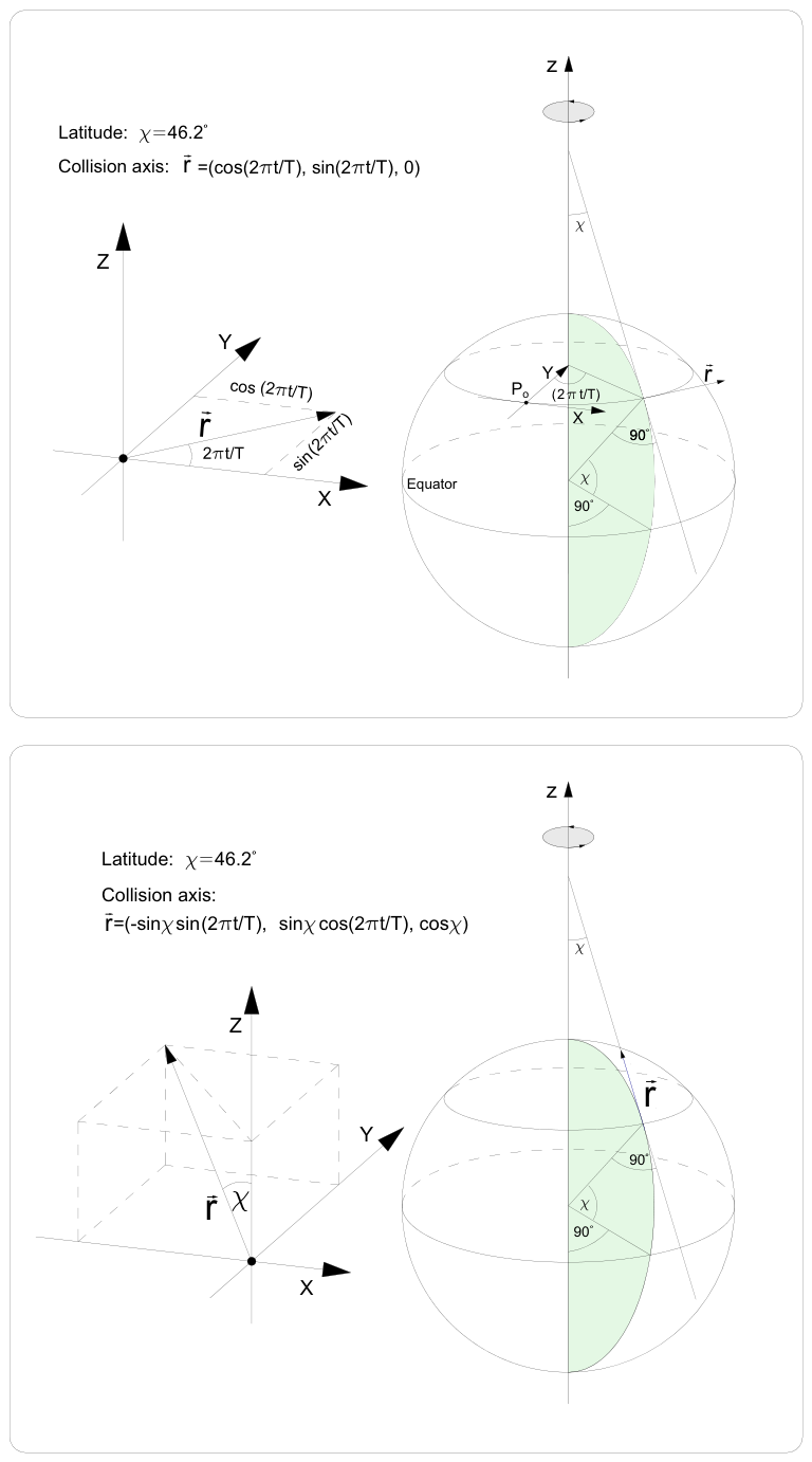
where $\overrightarrow{r}$ is the unit vector along the collision axis, aligned with the detector axis. Since we have introduced $\overrightarrow{r},$ let us parametrize it before proceeding further. Earth rotates with a period of approximately 24 h around its axis, and therefore $\overrightarrow{r}$ also changes with Earth’s rotation in the global reference frame. If we align the global reference frame’s z-axis parallel to Earth’s rotational axis, then (see Appendix A)

$$\overrightarrow{r}=(\sin \lambda \cos (2\pi t/T),\sin \lambda \sin (2\pi t/T),\cos \lambda )$$

(19)

where $\lambda$ is the angle between the LHC beam (collision) axis and the Earth’s rotational axis. For ATLAS and CMS, whose beam directions are approximately aligned along the east–west direction (i.e., nearly perpendicular to the Earth’s meridians), this angle is close to 90° (with a small deviation of order 10°, which is not essential for our purposes. Deviations from this approximation will be specified if relevant). For a general detector at CERN, $\lambda$ depends on the local beam orientation, with the minimum value corresponding to the meridian (north–south) direction and given by CERN’s latitude, $\chi$ ≃ 46.2°. Here, T denotes the Earth’s rotation period. This form of $\overrightarrow{r}$ is straightforward to interpret: the component parallel to the rotational axis remains constant, while the perpendicular component rotates with the Earth’s period. In this parametrization, $\overrightarrow{r}$ coincides with the x-axis when $\lambda =\pi /2$ and $t=0$ (the beginning of the day).

At very high energies, the proton mass can be neglected, so $E\approx P$ (half of the center of mass energy). The momentum of the intermediate boson is then

$$\begin{array}{cc}\hfill Q_{\mu }& =E\left(\right(x_1+x_2),(x_1-x_2\left)\overrightarrow{r}\right)\hfill \end{array}$$

(20)

$$\begin{array}{cc}\hfill Q^2& =4x_1{x}_2{E}^2\hfill \end{array}$$

(21)

In the literature, it is common to parametrize Q in terms of invariant mass M and rapidity Y

$$Q_{\mu }=M(\cosh Y,\overrightarrow{r}\sinh Y),Q^2=M^2$$

(22)

which relates $x_{1,2}$ to M and Y:

$$x_{1,2}={\displaystyle \frac{M}{2E}}\exp (\pm Y)$$

(23)

The Jacobian

$${\displaystyle \frac{\partial (M^2,Y)}{\partial (x_1,x_2)}}=4E^2$$

(24)

allows the differential cross-section to be written as

$${\displaystyle \frac{d^2{\sigma }_p}{d{M}^{2}dY}}=\sum _f{\displaystyle \frac{f_{qf}\left(x_1\right)f_{\overline{q}f}\left(x_2\right)}{4E^2}}{\sigma }_f$$

(25)

where ${\sigma }_p$ and ${\sigma }_f$ denote the proton level and parton-level cross-sections, respectively:

$$\begin{array}{cc}\hfill {\sigma }_p& =\sigma (pr\left(P_1\right)+pr\left(P_2\right)\to l+\overline{l})\hfill \end{array}$$

(26)

$$\begin{array}{cc}\hfill {\sigma }_f& =\sigma (q_f\left(x_1{P}_1\right)+{\overline{q}}_f\left(x_2{P}_2\right)\to l+\overline{l})\hfill \end{array}$$

(27)

A straightforward calculation of ${\sigma }_f$ yields [13]

$$\begin{array}{cc}\hfill {\sigma }_f& ={\sigma }_{EM}[1+{\displaystyle \frac{g_f{g}_l\left(M^2-M_{eff}^2(1-{\Gamma }_{0SM}^2/4M_Z^2)\right)}{2\left|e_f\right|M^2{\sin }^{2}2{\theta }_w}}R\left(M^2\right)\hfill \\ & +{\displaystyle \frac{(1+g_f^2)(1+g_l^2)}{16e_f^2{\sin }^{4}2{\theta }_w}}R\left(M^2\right)]\hfill \end{array}$$

(28)

$$\begin{array}{cc}\hfill {\sigma }_{EM}& ={\displaystyle \frac{4\pi {\alpha }^2}{9M^2}}{e}_f^2\hfill \end{array}$$

(29)

where $\left|e_f\right|$ equals to $2/3$ or $1/3$ for u and d quarks, respectively. Also, for the interaction constant $g_f$, we have $g_u=1-8/3{\sin }^2{\theta }_w$ and $g_d=1-4/3{\sin }^2{\theta }_w$. The resonance factor is

$$R\left(M^2\right)={\displaystyle \frac{M^4}{{\left(M^2-M_{eff}^2(1-{\Gamma }_{0SM}^2/4M_Z^2)\right)}^2+M_{eff}^4{\Gamma }_{0SM}^2/M_Z^2}}$$

(30)

From the cross-section and the form of $R\left(M^2\right)$, we see clearly how the resonance behavior is modified by LIV. The resonance mass $M_r$ and peak cross-section ${\sigma }_{f\max }$ are shifted:

$$\begin{array}{cc}\hfill M_r^2& =M_{eff}^2(1-{\Gamma }_{0SM}^2/4M_Z^2)\hfill \end{array}$$

(31)

$$\begin{array}{cc}\hfill & \approx M_Z^2\left(1-{\delta }_{LIV}{(n_0\cosh Y-\left(\overrightarrow{n}·\overrightarrow{r}\right)\sinh Y)}^2\right)(1-{\Gamma }_{0SM}^2/4M_Z^2)\hfill \end{array}$$

(32)

$${\sigma }_{f\max }\approx {\sigma }_{f\max }^{LI}(1-{\displaystyle \frac{{\delta }_{LIV}{(n_0\cosh Y-\left(\overrightarrow{n}·\overrightarrow{r}\right)\sinh Y)}^2}{M_Z^2}})$$

(33)

Here the subdominant photon contribution is neglected in the ${\sigma }_{f\max }$.

For specific violation cases:

1. $n_0=1$, $\overrightarrow{n}=0$ for pure timelike cases;

2. $n_0=0$, ${\overrightarrow{n}}^2=1$ for pure spacelike cases;

3. ${\overrightarrow{n}}^2=n_0^2$ for lightlike cases.

• The corresponding parametrization of $n_0$, $\overrightarrow{n}$ can be applied. In a timelike case, the LIV effect is isotropic, while spacelike and lightlike violations produce anisotropic behavior. The resonance mass shift also depends on the sign of ${\delta }_{LIV}$: for the positive ${\delta }_{LIV}$ the resonance mass shifts below $M_Z$ and the peak sharpness decreases; for negative ${\delta }_{LIV}$, the opposite occurs.

For timelike violations, the shift can be compared to the experimental accuracy of the $M_Z$ measurement ( $\Delta M_Z\approx 2$ MeV), yielding

$${\delta }_{LIV}\le {\displaystyle \frac{2\Delta M_Z}{M_Z{\cosh }^{2}Y}}$$

(34)

which for $Y=5$ gives ${\delta }_{LIV}\sim {10}^{-8}-{10}^{-9}$.

3.2. Experimental Analyses of Parton-Level Cross-Section

As evident from the form of the differential cross-section, any potential LIV effects depend crucially on two main factors: the rapidity of the produced Z boson and the orientation of the collider experiment relative to the preferred direction set by the LIV vector. This strong dependence arises because the momentum of the intermediate Z boson is aligned almost perfectly with the beam (detector) axis in the laboratory frame.

In the case of spacelike and lightlike LIV, the signal exhibits a pronounced anisotropy. As a result, the observable acquires a modulation with sidereal time. This modulation occurs because the spatial component of the LIV vector is fixed with respect to a global, non-rotating reference frame (aligned with the distant stars). Consequently, the daily rotation of the Earth causes the orientation of any terrestrial detector to vary periodically relative to this frame, imprinting a sidereal-time dependence on the measured signal.

The key requirement for observing LIV signatures is the selection of high-rapidity events. The magnitude of the LIV correction grows almost exponentially with increasing rapidity, while for events near central or low rapidities, the effect remains extremely small; even the underlying anisotropy is negligible. However, high-rapidity events constitute only a small fraction of the total dataset compared with the dominant low-rapidity sample. Without separating them, the LIV contribution is strongly diluted by the bulk of unaffected events, resulting in only a marginal and currently undetectable distortion of the overall cross-section at present collider energies. Therefore, the optimal approach is to bin the data according to the Z-boson rapidity, thereby enhancing the sensitivity to possible LIV effects.

For the timelike class of LIV, rapidity binning alone is sufficient. In this scenario, searches for anisotropy or sidereal modulation are not required. Each rapidity bin then benefits from improved statistical power, and a careful examination of the resonance peak’s position, shape, and height provides robust constraints on the LIV parameter.

In contrast, spacelike and lightlike violations necessitate an additional binning in sidereal time. We propose dividing the data into N equal time intervals, each of width $\Delta t=D_s/N$, where $D_s\approx 86164.0905$ s corresponds to the length of a sidereal day. This choice ensures that the bins remain phase-locked to the celestial (stellar) reference frame, so that each bin corresponds to a fixed orientation of the experiment relative to the preferred LIV direction. In practice, narrower time bins improve the angular resolution of the anisotropy but reduce the number of events per bin—particularly at high rapidity, where statistics are already limited. The analysis must therefore strike an optimal balance between time-bin width and event statistics to maximize overall sensitivity.

3.2.1. Case of Timelike LIV

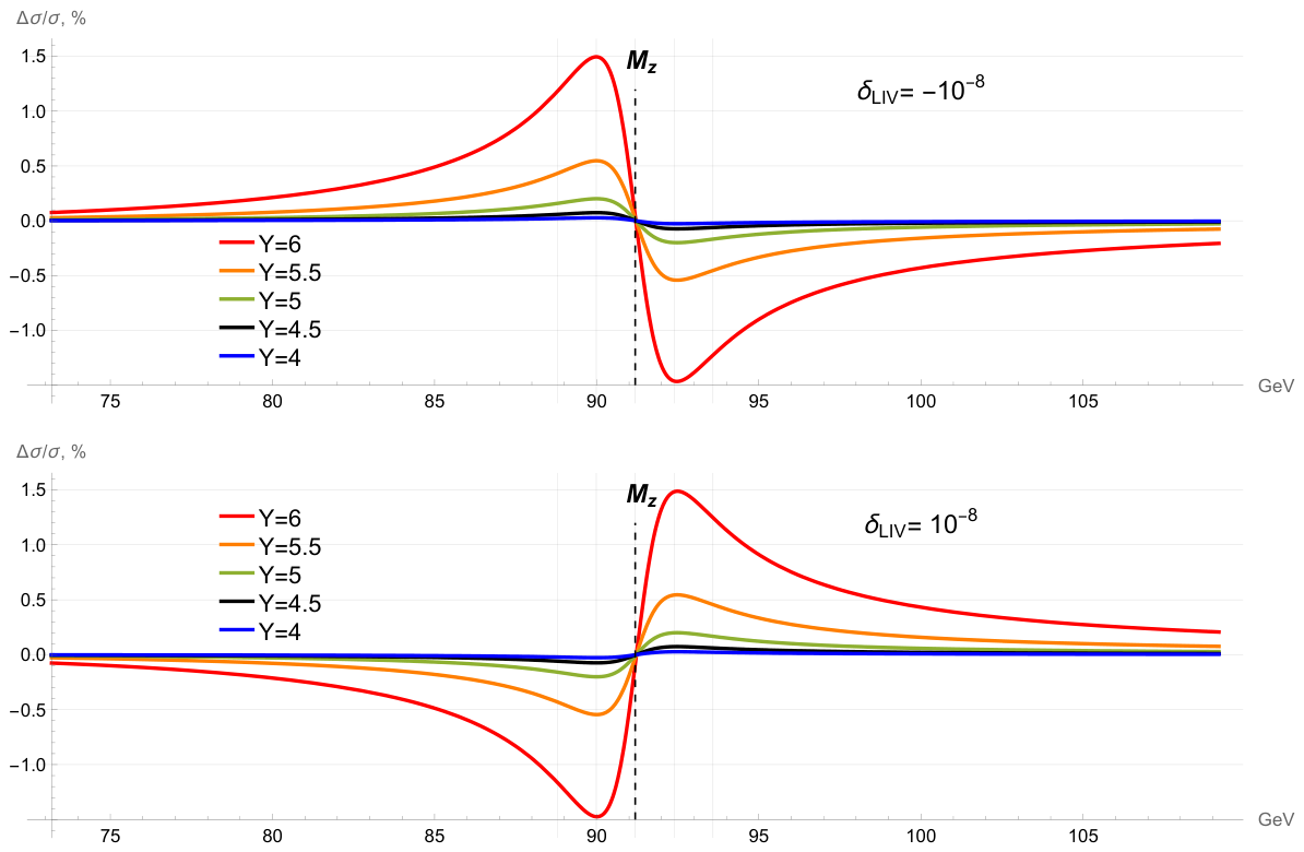
Let us first analyze timelike LIV as the simpler case study. To isolate the LIV contribution, we examine the relative difference between the LIV-modified parton-level cross-section (28) and its standard LI counterpart, evaluated for $\left|{\delta }_{\mathrm{LIV}}\right|={10}^{-8}$, as shown in Figure 1.

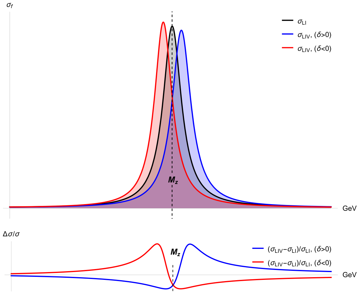
Although Figure 1 is constructed using the parton-level cross-section, the same qualitative behavior holds for the full proton-level differential cross section. The difference between the two arises solely from Lorentz-invariant factors associated with the parton distribution functions. The figure also demonstrates the role of the sign of ${\delta }_{LIV}$: the magnitude of the correction is nearly identical for both cases, but the signs differ.

The LIV effects reach their maximum deviation from the Lorentz-invariant case within the resonance region and diminish rapidly away from it. For the representative value $\left|{\delta }_{LIV}\right|={10}^{-8}$ used in the plot, the relative correction amounts to a few tenths of a percent at rapidity $Y=5$ and rises to approximately 1.5% at $Y=6$—a regime accessible at future high-energy colliders. Even smaller effects on the order of 0.2% can still be statistically significant given the precision of modern measurements. Although these deviations are too subtle to discern clearly on the scale of the printed figure, we provide an exaggerated version Figure 2 to better illustrate the structure of the LIV correction relative to the standard Lorentz-invariant parton-level cross-section.

As noted earlier, although the LIV contribution may become substantial at high rapidities, such events are relatively rare. In a typical experimental dataset, events from all rapidities are combined without separation. Consequently, the majority of the sample consists of low-rapidity events carrying a negligible LIV component. The small, perturbative nature of the LIV correction precludes large distortions of the overall lineshape, even more so if an analysis team fits this mixed dataset assuming purely Standard Model (Lorentz-invariant) physics. The fit primarily absorbs the effect through a systematic shift in the extracted resonance mass (and, to a lesser extent, in the effective width), as these parameters govern the position and overall profile of the peak, but at an unidentifiable level.

To quantify this behavior, we have computed the absolute shift $\Delta M_Z$ in the reconstructed Z-boson mass for various mixtures of LI and LIV events at different rapidities. The results are presented in

Table 1. Absolute mass shift $|\Delta M_Z|$ as a function of rapidity Y and the fractional composition of LI and LIV contributions in the data.

LI	100%	80%	60%	50%	40%	20%	0%
LIV	0%	20%	40%	50%	60%	80%	100%
Y = 0	0 eV	0.1 keV	0.2 keV	0.3 keV	0.3 keV	0.5 keV	0.6 keV
Y = 2	0 eV	1.3 keV	2.6 keV	3.2 keV	3.9 keV	5.2 keV	6.5 keV
Y = 4	0 eV	68 keV	136 keV	170 keV	204 keV	272 keV	340 keV
Y = 4.5	0 eV	185 keV	370 keV	462 keV	0.6 MeV	0.7 MeV	0.9 MeV
Y = 5	0 eV	0.5 MeV	1.0 MeV	1.3 MeV	1.5 MeV	2.0 MeV	2.5 MeV
Y = 6	0 eV	3.7 MeV	7.4 MeV	9.3 MeV	11.1 MeV	14.8 MeV	18.6 MeV

This table shows resonance mass shifts obtained when the ${\sigma }_{LIV}$ cross-section is reconstructed using a Standard Model fit. “LI” denotes the Lorentz-invariant cross-section, while “LIV” denotes the Lorentz-violating contribution. Cross-sections are assumed at the parton level according to formula (28), with photon contributions included though subdominant. The data is simplified to a mixture of LI and LIV events: low-rapidity events remain close to the Standard Model, while high-rapidity events exhibit detectable LIV effects as resonance mass shifts. The magnitude of the shift scales with the level of LIV contamination. The sign of ${\delta }_{LIV}$ leads to either overestimation (${\delta }_{LIV}>0$) or underestimation (${\delta }_{LIV}<0$) of the resonance mass, but differences remain within the displayed precision, so both cases are combined here. These resonance mass shifts arise within a standard analysis framework because an LI cross-section function is fitted to an LIV-distorted distribution. LIV contamination thus biases the fitted parameters of conventional methods. Here and everywhere below, the actual fitting was performed using Wolfram Mathematica’s NonlinearModelFit around the central values of 2.5 GeV for the decay rate and 91 GeV for the boson mass. The fit was performed in the mass interval $80\mathrm{GeV}<M<100\mathrm{GeV}$, with M and $\Gamma$ treated as floating parameters while the remaining input parameters were fixed. Synthetic data were first generated using the full distribution function with added random noise to simulate experimental variation. A nonlinear regression was then performed to fit these data to the LI distribution model to extract parameters $\Gamma$ and M, utilizing the NonlinearModelFit routine in Wolfram Mathematica.

.

The table confirms the trend discussed previously: at low rapidities the shift remains undetectable, while at high rapidities it becomes appreciable. For a realistic mixture of 90% LI and 10% LIV events at $Y=5$ (an experimentally accessible value), the induced mass shift is $\Delta M_Z\approx 0.25$ MeV. In contrast, when only pure LIV events at the same rapidity are considered, the shift increases to $\Delta M_Z\approx 2.5$ MeV. This value already exceeds the declared experimental uncertainty of 2.1 MeV reported by both the Tevatron and LHC collaborations. The effect is naturally more pronounced—and easier to detect—at even higher rapidities that are not yet available with present accelerators. With all that said, $Y=5$ is theoretically accessible but practically limited. The event numbers are much smaller, and various types of uncertainties increase. Detectors reliably measure Z boson events up to $\left|Y\right|\approx 3.5$ with high efficiency (>90% in central regions, $\left|\eta \right|<2.5$), but the efficiency decreases in forward regions ($\left|\eta \right|>2.5$). In addition, the accuracy of PDFs is lower for high-energy partons. Some of these problems can be partially mitigated in binned analyses, while others are difficult to address. It is difficult at this stage to quantify the uncertainty, but these are known issues [20,21]. Realistically, without binning, if a mixture of LIV events with $Y>4$ constitutes about $10\%$, we can expect an effect of the order $0.1$–$0.25$ MeV. If only events with $Y>4$ are lumped together, then the expected effects should lie in the range $0.34$–$2.5$ MeV.

For any fixed rapidity, the mass shift is well approximated by the simple analytic relation

$$\Delta M_z={\displaystyle \frac{{\delta }_{LIV}}{2}}{M}_Z{\cosh }^{2}Y$$

(35)

The table serves as a proxy that effectively mimics the impact of parton distribution functions in a simplified manner. Even within this approximation, the essential features of the LIV effect are clearly illustrated. More exact calculations incorporating realistic PDFs, next-to-leading-order QCD or electroweak corrections, or different treatments of the propagator pole (such as running-width or complex-mass schemes) would not change the qualitative behavior, nor could they be easily mistaken for an LIV signal—although they would provide a more quantitatively precise prediction.

In standard inclusive analyses, the limited fraction of high-rapidity events typically results in only marginal effects. However, when data at $Y\approx 4.5$ are analyzed in separate rapidity bins, the LIV signature becomes distinctly visible for $\left|{\delta }_{LIV}\right|={10}^{-8}$ and potentially even for $\left|{\delta }_{LIV}\right|={10}^{-9}$. Should LIV exist at this level, next-generation accelerators (where effects at $Y\ge 6$ grow highly pronounced) would likely observe it unambiguously. Nevertheless, the present analysis remains valuable for existing colliders: the predicted mass shifts lie at the edge of current measurement precision and enable new consistency checks by comparing results from machines operating at different center-of-mass energies, such as the Tevatron and the LHC.

3.2.2. Case of Spacelike LIV

We have already emphasized the importance of rapidity binning for LIV detection. Therefore, when discussing spacelike LIV in this subsection and lightlike LIV in the next, we will not revisit those points. Instead, we assume that Y-binning has been applied to the selected rapidities and focus on how the LIV signal should manifest.

The resonance value $M_r$ for spacelike LIV, according to (32), if we parametrize the LIV vector in the global reference frame as

$$n_0=0,\overrightarrow{n}=(\sin \alpha \cos \beta ,\sin \alpha \sin \beta ,\cos \alpha )$$

(36)

takes the form

$$\begin{array}{cc}\hfill M_r^2& \approx M_Z^2\left(1-{\delta }_{LIV}{\left(\overrightarrow{n}·\overrightarrow{r}\right)}^2{\sinh }^{2}Y\right)(1-{\Gamma }_{0SM}^2/4M_Z^2)\hfill \end{array}$$

(37)

$$\begin{array}{cc}\hfill \overrightarrow{n}·\overrightarrow{r}& =\sin \alpha \sin \lambda \cos (2\pi t/T-\beta )+\cos \alpha \cos \lambda \hfill \end{array}$$

(38)

and

$$\Delta M_z={\displaystyle \frac{{\delta }_{LIV}}{2}}{M}_Z{\sinh }^{2}Y{\left(\overrightarrow{n}·\overrightarrow{r}\right)}^2=\Delta M_{z,\mathrm{timelike}}{\tanh }^{2}Y{\left(\overrightarrow{n}·\overrightarrow{r}\right)}^2$$

(39)

$\Delta M_{z,\mathrm{timelike}}$ is shift corresponding to timelike violation for the same Y and ${\delta }_{LIV}$. For high rapidities ${\tanh }^{2}Y\approx 1$.

An interesting observation emerges: if $\overrightarrow{n}$ is parallel or antiparallel to Earth’s rotational axis, then

$$\Delta M_z\approx \Delta M_{z,\mathrm{timelike}}{\cos }^2\lambda$$

(40)

In this case, due to the the residual rotational symmetry in planes orthogonal to $\overrightarrow{n}$, the experimental signature appears isotropic, similar to the timelike violation scenario. However, for experiments with different orientations or locations, the magnitude of the LIV effect can vary. For example, ATLAS and CMS have approximately the same value of ${\cos }^2\lambda$ due to the LHC geometry. Their beam axes are nearly perpendicular to the Earth’s meridians, corresponding to $\lambda$ ≃ 90°, and are therefore suppressed. In contrast, when $\lambda$ coincides with CERN’s latitude, $\chi$ ≃ 46.2°, one finds ${\cos }^2\lambda \approx 0.48$, so that for the same ${\delta }_{\mathrm{LIV}}$, the effect is approximately half as large as in the timelike case.

Another simple case to analyze is when $\overrightarrow{n}$ is orthogonal to Earth’s rotational axis:

$$\begin{array}{cc}\hfill M_r^2& \approx M_Z^2\left(1-{\delta }_{LIV}{\sin }^2{\lambda \cos }^2(2\pi t/T-\beta ){\sinh }^{2}Y\right)(1-{\Gamma }_{0SM}^2/4M_Z^2)\hfill \end{array}$$

(41)

$$\begin{array}{cc}\hfill \Delta M_z& \approx \Delta M_{z,\mathrm{timelike}}{\sin }^2{\lambda \cos }^2(2\pi t/T-\beta )\hfill \end{array}$$

(42)

Here, for a given rapidity, the maximum LIV deviation occurs at $2\pi t/T-\beta =k\pi$ ($k\in \mathbb{Z}$). The maximum deviation is approximately ${\sin }^2\lambda$ times as large as in the timelike LIV case. If sidereal-time binning is not used in the data analysis, the observed resonance mass shift (for the same ${\delta }_{LIV}$ values considered earlier) is further suppressed by a factor of $1/2$, since ${\cos }^2$ is averaged over time. For $\left|Y\right|=5$, $\lambda =\chi$ ≃ 46.2°, and $|{\delta }_{\mathrm{LIV}}|={10}^{-8}$, we obtain $\Delta M_Z\approx 0.65\mathrm{MeV}$ without sidereal-time binning. For ATLAS and CMS, where $\lambda$ is close to 90°, one finds $\Delta M_Z\approx 1.3\mathrm{MeV}$. With sidereal-time binning and for selected rapidities, the direction of the LIV vector $\overrightarrow{n}$ can be inferred by identifying when $\Delta M_Z$ reaches its maximum.

Below we provide the table of $\Delta M_Z$ for different values of $\alpha$, without applying time binning, for the case $\left|Y\right|=5$ and $\left|{\delta }_{LIV}\right|={10}^{-8}$, for $\lambda$ ≈ 46.2°.

In

Table 2. Reconstructed mass shifts $\Delta M_z$ without time binning for spacelike LIV.

$\mathit{\alpha }$	0	$\mathit{\pi }/8$	$\mathit{\pi }/4$	$3\mathit{\pi }/8$	$\mathit{\pi }/2$	$5\mathit{\pi }/8$	$3\mathit{\pi }/4$	$7\mathit{\pi }/8$	$\mathit{\pi }$
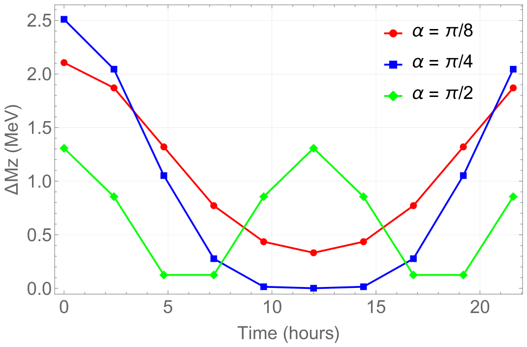
$\Delta M_z$ (MeV)	1.2	1.1	0.9	0.7	0.7	0.7	0.9	1.1	1.2

, our expectations are confirmed. The size of the LIV effect is mitigated due to the averaging factor from Earth’s rotation. However, when sidereal-time binning is applied, the situation changes. With sufficient statistics, sidereal modulation helps to identify the preferred direction through the peak value of the LIV effect, which can be as significant as in the timelike LIV case. See Figure 3.

3.2.3. Case of Lightlike LIV

The lightlike violation shares certain features with both timelike and spacelike violation, but also possesses distinct characteristics. If we parametrize the lightlike $n_{\mu }$ vector in the global reference frame, similar to (36), we write $n_{\mu }=(\pm 1,\overrightarrow{n})$. The sign in front of the time component affects only one specific case, which we will discuss later. What truly matters in this context is whether, in $n_{\mu }=(n_0,\overrightarrow{n})$, the time and space components have the same or opposite signs, not which component is individually positive or negative. For the moment, let us choose the positive sign for the time component and proceed with this choice.

The resonance value is then

$$\begin{array}{cc}\hfill M_r^2& \approx M_Z^2\left(1-{\delta }_{LIV}{(\cosh Y-\left(\overrightarrow{n}·\overrightarrow{r}\right)\sinh Y)}^2\right)(1-{\Gamma }_{0SM}^2/4M_Z^2)\hfill \end{array}$$

(43)

where $\overrightarrow{n}·\overrightarrow{r}$ is defined in (38). Since at high rapidities $\cosh Y\approx \pm \sinh Y$ for positive and negative Y, respectively, this simplifies to

$$M_r^2\approx M_Z^2\left(1-{\delta }_{LIV}{\cosh }^2{Y(1\mp \overrightarrow{n}·\overrightarrow{r})}^2\right)(1-{\Gamma }_{0SM}^2/4M_Z^2)$$

(44)

indicating that for positive Y, the LIV effect is partially cancelled, while for negative Y it is amplified by up to a factor of four, potentially yielding a stronger signal than in the timelike violation case.

Similarly to spacelike violation, there is a specific case worth attention and simpler to analyze. If $\overrightarrow{n}$ is parallel to Earth’s rotational axis, then the corresponding shift in the resonance mass is

$$\Delta M_z\approx \Delta M_{z,\mathrm{timelike}}{(1\mp \cos \lambda )}^2$$

with the minus sign corresponding to positive rapidity and the plus sign to negative rapidity. For $\lambda =\chi$, when the positive and negative rapidities are analyzed separately, the reconstructed mass shifts are

$$\begin{array}{cc}\hfill \mathrm{when}Y& >0,\Delta M_z\approx 0.1\Delta M_{z,\mathrm{timelike}}\hfill \end{array}$$

(45)

$$\begin{array}{cc}\hfill \mathrm{when}Y& <0,\Delta M_z\approx 3\Delta M_{z,\mathrm{timelike}}\hfill \end{array}$$

(46)

This indicates that the LIV effect is suppressed at current experiment energies for $Y>0$, but becomes approximately three times larger than the timelike LIV case for $Y<0$. For $\lambda$ ≃ 90°, which approximately corresponds to the ATLAS/CMS orientation, the mass shift satisfies $\Delta M_Z\approx \Delta M_{Z,\mathrm{timelike}}$. If $\overrightarrow{n}$ is antiparallel to the Earth’s rotational axis, the results for positive and negative rapidities are interchanged. The same interchange occurs if the sign of the time component is reversed, $n_{\mu }=(-1,\overrightarrow{n})$, or equivalently $n_{\mu }=(1,-\overrightarrow{n})$. This dependence on the sign of the rapidity, i.e., on the direction of the intermediate Z-boson three-momentum, is a distinctive feature of pure lightlike violations and does not arise in timelike or spacelike LIV.

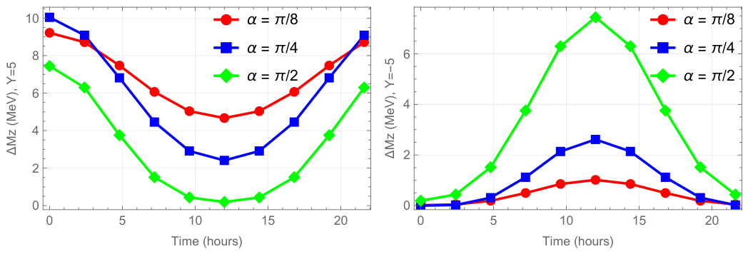
Below we provide a table of $\Delta M_Z$ values for a general lightlike violation, reconstructed without time binning. In addition, we graph how $\Delta M_Z$ changes when data is segregated by time to have side by side comparison.

As we see from

Table 3. Reconstructed mass shifts $\Delta M_z$ without time binning for lightlike LIV. $\left|Y\right|=5$, $|{\delta }_{\mathrm{LIV}}|={10}^{-8}$, $\lambda =\chi$.

$\mathit{\alpha }$	0	$\mathit{\pi }/8$	$2\mathit{\pi }/8$	$3\mathit{\pi }/8$	$4\mathit{\pi }/8$	$5\mathit{\pi }/8$	$6\mathit{\pi }/8$	$7\mathit{\pi }/8$	$\mathit{\pi }$
$\Delta M_Z$ (MeV), $Y=5$	7.2	6.8	5.9	4.6	3.2	1.9	1	0.4	0.2
$\Delta M_Z$ (MeV), $Y=-5$	0.2	0.4	1	1.9	3.2	4.6	5.9	6.8	7.2

and Figure 4, the average mass-shift value due to the Earth’s rotation is not significantly suppressed for certain special configurations of the LIV vector, the detector, and the Earth’s rotational axis. However, for other configurations, the effect becomes undetectable. Once sidereal modulations are studied, however, the LIV effect becomes unavoidable in all cases, whether at positive or negative rapidities.

4. Discussion and Conclusions

Our analysis focused primarily on the Z boson, whose narrow width and clean leptonic channels make it an ideal probe of LIV. The modified dispersion relation affects the resonance shape most strongly at high rapidities. Although the absolute magnitude of the LIV effect can be sizable, its impact is diluted in global fits, since only a small fraction of events populate the high-rapidity region. This motivates dedicated analyses that isolate high-rapidity bins and, in anisotropic scenarios, employ separate binning in sidereal time. Although practical limitations such as statistics may arise, the potential sensitivity justifies such targeted studies.

The behavior in the timelike, spacelike, and lightlike cases is qualitatively distinct. In particular, spacelike and lightlike configurations introduce anisotropy, which not only leads to sidereal modulation but also makes the signal dependent on the detector location and orientation. For example, if the spacelike LIV vector is aligned with the Earth’s rotational axis, experiments such as ATLAS or CMS would be insensitive to the effect, while differently oriented or located experiments could still observe it. The LIV effect is generally strongest in the lightlike case and weakest in the spacelike case.

When favorable geometric configurations allow for detection in anisotropic scenarios, the presence of LIV may be established even without sidereal binning. However, distinguishing it from the timelike case and identifying the preferred direction of the LIV vector requires measuring sidereal modulations.

An important caveat is that the Z boson is routinely used for calibration at hadron colliders. Whether this practice inadvertently biases against possible LIV effects remains an open question. Nonetheless, the Z boson remains a uniquely clean candidate for such searches.

The same reasoning extends naturally to the W boson. Recent tensions between Tevatron and LHC measurements of $M_W$, with discrepancies at the level of 65 MeV [22,23], are qualitatively consistent with LIV behavior for negative ${\delta }_{LIV}$. However, to fully explain this discrepancy, the corresponding $\delta$ parameter would need to be a few orders of magnitude larger than considered here. How justified such a difference between the weak bosons is depends on how closely LIV respects the weak symmetry. Phenomenologically, we can state that the photon and Z boson LIV parameters are correlated, as they are orthogonal mass states of the original $SU\left(2\right)$ and $U{\left(1\right)}_Y$ neutral gauge bosons, and for the photon LIV is practically zero. Thus, if $SU\left(2\right)$ is respected, then ${\delta }_Z={\delta }_W{\displaystyle \frac{\cos 2{\theta }_w}{{\cos }^2{\theta }_w}}\approx 0.7{\delta }_W$ [24,25]; if not, then there can be no correlation between them. While experimental systematics may ultimately explain the difference, the possibility of LIV contributing to such anomalies warrants serious consideration.

Taken together, the Z and W bosons highlight how collider observables provide a complementary window on LIV, distinct from astrophysical probes. Our study shows that LIV effects scale strongly with rapidity, can introduce sidereal modulations in anisotropic cases, and may lead to percent-level modifications of cross-sections for $\left|{\delta }_{LIV}\right|\sim {10}^{-8}$. These translate into effective shifts in fitted resonance masses that exceed current experimental uncertainties.

In outlook, collider studies of unstable bosons offer sensitivity to LIV at the ${10}^{-8}$ (may be even at ${10}^{-9}$) level, competitive with astrophysical bounds but in a sector inaccessible to astrophysical observations. Pursuing dedicated rapidity and sidereal-time analyses and extending the framework to W bosons could therefore open a new experimental window on fundamental physics beyond the Standard Model.

References

Kostelecky, A.; Russell, N. Data Tables for Lorentz and CPT Violation. Rev. Mod. Phys.2011, 83, 11. [Google Scholar] [CrossRef] [Scilit]
Takeda, M.; Hayashida, N.; Honda, K.; Inoue, N.; Kadota, K.; Kakimoto, F.; Kamata, K.; Kawaguchi, S.; Kawasaki, Y.; Kawasumi, N.; et al. Extension of the Cosmic-Ray Energy Spectrum beyond the Predicted Greisen-Zatsepin-Kuz’min Cutoff. Phys. Rev. Lett.1998, 81, 1163–1166. [Google Scholar] [CrossRef] [Scilit]
Takeda, M.; Hayashida, N.; Honda, K.; Inoue, N.; Kadota, K.; Kakimoto, F.; Kamata, K.; Kawaguchi, S.; Kawasaki, Y.; Kawasumi, N.; et al. Energy determination in the Akeno Giant Air Shower Array experiment. Astropart. Phys.2003, 19, 447–462. [Google Scholar] [CrossRef] [Scilit]
The Pierre Auger Collaboration. Features of the energy spectrum of cosmic rays above 2.5 ∗ 1018 eV using the Pierre Auger Observatory. Phys. Rev. Lett.2020, 125, 121106. [Google Scholar] [CrossRef] [Scilit]
The Pierre Auger Collaboration. Measurement of the cosmic-ray energy spectrum above 2.5 ∗ 1018 eV using the Pierre Auger Observatory. Phys. Rev. D2020, 102, 062005. [Google Scholar] [CrossRef] [Scilit]
The Pierre Auger Collaboration. The energy spectrum of cosmic rays beyond the turn-down around 1017 eV as measured with the surface detector of the Pierre Auger Observatory. Eur. Phys. J. C2021, 81, 966. [Google Scholar] [CrossRef] [Scilit]
Zatsepin, G.T.; Kuz’min, V.A. Upper limit of the spectrum of cosmic rays. JETP Lett.1966, 41, 78. [Google Scholar]
Chkareuli, J.L.; Kepuladze, Z.; Tatishvili, G. Spontaneous Lorentz Violation via QED with Non-Exact Gauge Invariance. Eur. Phys. J. C2008, 55, 309–316. [Google Scholar] [CrossRef] [Scilit]
Chkareuli, J.L.; Kepuladze, Z. Standard model with partial gauge invariance. Eur. Phys. J. C2012, 72, 1954. [Google Scholar] [CrossRef] [Scilit]
Moura, C.A.; Quintino, L.; Rossi-Torres, F. Analyzing the Time Spectrum of Supernova Neutrinos to Constrain Their Effective Mass or Lorentz Invariance Violation. Universe2023, 9, 259. [Google Scholar] [CrossRef] [Scilit]
Kepuladze, Z. Lorentz Violation: Loop-Induced Effects in QED and Observational Constraints. arXiv2025, arXiv:2504.15608. [Google Scholar] [CrossRef] [Scilit]
Jejelava, J.; Kepuladze, Z. Probing Lorentz Invariance Violation in Z Boson Mass Measurements at High-Energy Colliders. Phys. Rev. D2026, 113, 075011. [Google Scholar] [CrossRef] [Scilit]
Jejelava, J.; Kepuladze, Z. Probing Lorentz Invariance Violation at High-Energy Colliders via Intermediate Massive Boson Mass Measurements: Z Boson Example. In Proceedings of the 28th Workshop “What Comes Beyond the Standard Models”, Bled, Slovenia, 6–17 July 2025. [Google Scholar] [CrossRef] [Scilit]
CMS Collaboration. Searches for violation of Lorentz invariance in top quark pair production using dilepton events in 13 TeV proton-proton collisions. Phys. Lett. B2024, 857, 138979. [Google Scholar] [CrossRef] [Scilit]
Lunghi, E.; Sherrill, N.; Szczepaniak, A.; Vieira, A. Quark-sector Lorentz violation in Z-boson production. J. High Energy Phys.2024, 7, 167. [Google Scholar] [CrossRef] [Scilit]
Schael, S.; Barate, R.; Bruneliere, R.; Buskulic, D.; De, B.I.; Decamp, D.; Ghez, P.; Goy, C.; Jezequel, S.; Lees, J.P.; et al. Precision Electroweak Measurements on the Z Resonance. Phys. Rept.2006, 427, 257–454. [Google Scholar] [CrossRef] [Scilit]
Willenbrock, S. Mass and width of an unstable particle. Eur. Phys. J. Plus2024, 139, 523. [Google Scholar] [CrossRef] [Scilit]
Greiner, W.; Müller, B. Gauge Theory of Weak Interactions, 4th ed.; Springer: Berlin/Heidelberg, Germany, 2009. [Google Scholar]
CMS Collaboration. Measurements of differential Z boson production cross sections in proton-proton collisions at = 13 TeV. J. High Energy Phys.2019, 12, 61. [Google Scholar] [CrossRef] [Scilit]
LHCb Collaboration. Precision measurement of forward Z boson production in proton-proton collisions at = 13 TeV. J. High Energy Phys.2022, 7, 26. [Google Scholar] [CrossRef] [Scilit]
CDF Collaboration; Aaltonen, T.; Amerio, S.; Amidei, D.; Anastassov, A.; Annovi, A.; Antos, J.; Apollinari, G.; Appel, J.A.; Arisawa, T. High precision measurement of the W-boson mass with the CDF II detector. Science2022, 376, 170–176. [Google Scholar] [CrossRef] [Scilit]
CMS Collaboration. Measurement of the W Boson Mass in Proton-Proton Collisions at sqrts = 13 TeV, CMS-PAS-SMP-23-002. ATLAS Collaboration, Improved W Boson Mass Measurement Using 7 TeV Proton-Proton Collisions with the ATLAS Detector, ATLAS-CONF-2023-004, CERN, Geneva. 2023. Available online: https://cds.cern.ch/record/2853290 (accessed on 7 July 2026).
Colladay, D.; Noordmans, J.P.; Potting, R. CPT and Lorentz violation in the Photon and Z-boson sector. Symmetry2017, 9, 248. [Google Scholar] [CrossRef] [Scilit]
Lehnert, R. Constraining Lorentz Violation in Electroweak Physics. J. Phys. Conf. Ser.2018, 952, 012008. [Google Scholar] [CrossRef] [Scilit]
Figure 1.for the Drell–Yan process via neutral bosons. The plot shows the relative difference between (Lorentz-violating cross-section) and (Lorentz-invariant, i.e., Standard Model cross-section) at the parton level for . Plotting this difference highlights the structure of LIV. Although visually small, the effect is not exactly zero at the resonance point, as emphasized in Figure 2. The maximum deviation occurs about away from the true mass (). This should not be confused with the resonance mass shift , expected to be only a few MeV. The shift arises during standard fitting if the distorted LIV shape is not accounted for. The sign of determines whether the fitted mass is over- or underestimated relative to .
Figure 2.Highly exaggerated comparison of LIV and LI cross-sections for . This plot is for demonstrative purposes only. For the LHC data, the expected difference is limited to for the rapidity , rendering it practically indistinguishable by visual inspection alone.
Figure 3.Sidereal modulation of mass shift. This graph illustrates how the mass shift varies with sidereal time for three values of . The effect is largest when , reaching the level of the timelike violation. We set ; the angle does not affect the magnitude of the mass shift but shifts the phase of the sidereal modulation, moving its maximum from to . As in the table above, , , and ≃ 46.2°. The qualitative behavior remains the same for other values of , with only the relative amplitudes for different changing.
Figure 4.Sidereal modulation of mass shift. These graphs, similar to the spacelike LIV case, illustrate how the mass shift varies with sidereal time for three different values of at both positive and negative rapidities. The characteristic difference of the LIV effect is clearly visible in both the behavior and the amplitude between the two rapidity signs. As discussed earlier, the maximal effect can reach up to four times that of the timelike LIV contribution. In this example, , , and .