


Abstract
Climate change can impact various facets of a region’s fire regime, such as the frequency and timing of fire ignitions. This study examines the temporal trends of monthly fire counts in the Northwest and Northeast Regions of Ontario, Canada, between 1960 and 2023. Fires ignited by human activities or lightning are analyzed separately. The significance of historical trends is investigated using the Cochrane–Orcutt method, which identifies decreasing trends in the number of human-caused fires for several months, including May through July. A complementary trend analysis of total area burned is also conducted. The forecasting of future months’ fire counts is explored using a Negative Binomial Autoregressive (NB-AR) model suitable for count time series data with overdispersion. In the NB-AR model, the use of climate teleconnections at a range of temporal lags as predictors is investigated, and their predictive skill is quantified through cross-validation estimates of Mean Absolute Error on a testing dataset. Considered teleconnections include the El Niño-Southern Oscillation (ENSO), Pacific Decadal Oscillation (PDO), Arctic Oscillation (AO), North Atlantic Oscillation (NAO), and Atlantic Multidecadal Oscillation (AMO). The study finds the use of teleconnection predictors promising, with a notable benefit for forecasting human-caused fire counts but mixed results for forecasting lightning-caused fire counts.
1. Introduction
The structure and function of forests are influenced by fire, a natural phenomenon that is essential to the global environment [1]. Wildfires are caused by at least three factors: continuous fuels (vegetation), favorable weather, and an ignition source [2], with different ecosystems having different wildfire regimes [3]. Climate and weather variables such as wind, temperature, precipitation, and relative humidity are important determinants of the occurrence of fires and are the key components of Canada’s Fire Weather Index System [4]. For instance, fuel moisture is influenced by weather over short or extended periods of time, which directly impacts the ignition chance and potential hazard of wildfire. It is therefore natural that during fire seasons, weather is perhaps the best indicator of regional fire activity [5,6]. Of the mentioned weather variables, temperature is the most significant factor that influences the total annual activity of wildland fires, with warmer temperatures driving increased fire activity, although several factors of weather and climate similarly influence the growth of individual fires [7,8].
Fires have profound ecological impacts affecting ecosystems. Given these consequences, understanding changes in fire occurrence and behavior is important for effective management and mitigation. Indeed, recent studies have shown that shifts in fire regimes are occurring in response to a changing environment [9,10]. An increase in fire occurrence has been associated with drier and warmer conditions driven by climate change [11,12]. One way that climate change can impact fire occurrence is through relationships with climatic teleconnections [12]. Some sea surface temperature anomalies (SSTs) and climate teleconnections (TCs) relevant to North America include the Atlantic Multidecadal Oscillation (AMO), Arctic Oscillation (AO), North Atlantic Oscillation (NAO), El Niño-Southern Oscillation (ENSO), and Pacific Decadal Oscillation (PDO), which are known to influence weather on subcontinental to local scales [13].
Anomalies in the global pattern of SSTs and teleconnections during winter seasons are related to very wet and dry Canadian summers, which indirectly affect summer moisture availability and the occurrence of wildfires [14]. The AMO’s impacts occur primarily on the west coast and in the lower Great Lakes region of southern Ontario and central Quebec. It has a quasi-cycle of approximately 70 (50–90) years [15]. The AMO has two phases: warm and cold. Warmer SSTs circulate more moisture to tropical storms and hurricanes, which increases North Atlantic tropical cyclone activity [16]. The Great Lakes have warmer-than-normal surface air temperatures during the warm phase of the AMO [17], and the AMO is also linked to previous occurrences of significant droughts in the United States Midwest and Southwest, with droughts being more frequent or lasting longer when the AMO is warm [14,17].
Summertime temperature anomalies in the Northern Hemisphere are influenced by changes in the NAO and AO [18,19]. The PDO, interannual ENSO, and their interactions have a significant impact on the winter temperature and precipitation regimes [14,18,20,21]. Macias Fauria and Johnson [22] found a strong correlation between the PDO and the occurrence of large lightning-caused fires (≥200 ha) across Canadian and Alaskan forest regions. The fire dynamics were mostly antiphase, and the warm PDO regime improved the fire weather east of the Rocky Mountains and affected central Canada. Other studies [23,24] have also revealed that the warm phase of ENSO and the positive phase of PDO resulted in an increased burned area in western and northwestern Canada, with winter and spring PDO and the additive spring PDO/ENSO index having the most significant relationship. Furthermore, there is evidence that the frequency of large forest fires ignited during fire seasons is related to climate teleconnections such as the PDO and ENSO [19,23,24,25,26].
The operational fire season in Ontario, Canada, is legislatively defined as April 1 through October 31 [27], but the duration of the potential and observed fire seasons based on fire weather or ignitions vary year to year. Trend analyses have revealed that fire seasons in Ontario and other provinces in Canada are tending to start earlier and/or end later [28,29,30] raising the question of whether these changes reflect a true increase in the number of fires occurring in the early or late months of the fire season, or whether it is just a temporal shift in fire occurrence. Warmer temperatures lower the positions of the water table and fuel moisture, while increasing evapotranspiration, lightning activity, and lightning-caused ignitions, as well as the number of human-caused fires, which can prolong the fire season [10,31,32]. Even though Price and Rind [31] and Westerling et al. [10] primarily focused on the United States, their results are applicable to regions with similar climatic conditions, including parts of Canada, while Flannigan et al. [32] exclusively used Canadian data, providing direct evidence of climate-driven changes in fire activity in the region.
In the literature, historical fire records have been used to analyze trends in fire activity, with some studies focusing on human-caused fires, lightning-caused fires, or both. In Canada, approximately 50% of fires and 90% of the burned area are caused by lightning [29,30,33]. During extended periods of heightened fire risk when fuels are more flammable, human-caused fire ignitions are more common, extending the fire season [33]. Albert-Green et al. [29] examined trends in the start and end of the lightning-caused fire season in both Alberta and Ontario, focusing on the first Julian day each year when the estimated fire risk exceeds a probability threshold. In western Ontario, they found weak negative trends in the start date of the fire season but significant positive trends in the end date, concluding that there was a lengthening season. Specifically, the fire season ended 23, 22, and 21 days later over the 50-year period at the 1%, 5%, and 10% thresholds, respectively. Conversely, in eastern Ontario, the trends in start date were positive, implying that the season could be starting later in the year, but there was insufficient evidence to declare those trends significant. Meanwhile, trends in the end date for eastern Ontario were significant, but those trends were smaller than in the west, with the season ending approximately 2 weeks later at the 1% threshold over the 50 years of observed fire data.
Common trend analysis methods, such as the Mann–Kendall (MK) test [34,35] and the Theil–Sen (TS) slope estimator [36], have been used to investigate temporal trends in fire occurrence, focusing on the effects of climate change, to inform decisions on the level of intervention, planning, and policy adjustments or fire management agencies (e.g., [37,38,39,40,41]). The MK test evaluates the significance of monotonic trends in time series data, particularly in climatology and environmental analysis [42]. It is non-parametric, allowing for analysis without distributional assumptions, and can be applied to data over specific months, seasons, or decades. The TS slope estimator is also a non-parametric technique proposed by Theil [43] and modified by Sen [36] that can be used to quantify these trends. It is robust against outliers through its use of the median value of slopes calculated between all pairs of observed values. Jain et al. [37] analyzed the trends in fire season length and extreme fire weather in North America using the MK test and TS slope estimator. They found that the duration of the fire season was increasing in large areas of North America, especially in eastern Canada and the southwestern US. Ahmed and Hassan [39] studied trends in the number of forest fire occurrences, burned area, and seasonality of human- and lightning-caused fires in Alberta from 1959 to 2022, applying these analysis methods to examine patterns and magnitudes of these trends. They reported significant increases in the number of fires across nearly all natural subregions, particularly in both small (<200 ha) and large (≥200 ha) fire sizes, with the Alpine subregion being the only exception.
However, despite the wide use of MK, it may not always be the most appropriate choice of test. Positive autocorrelation in time series data increases the likelihood of detecting significant trends [44] and hence increases the probability of Type I Error (i.e., detecting a trend when there is none). To overcome this, methods such as the Cochrane–Orcutt (CO) method [45] and the trend-free pre-whitening Mann–Kendall test (TFPW-MK) [44] are used to improve the assessment of trend significance in serial correlated data. A modified form of the pre-whitening (PW) approach created by Kulkarni and Von Storch [46], the TFPW-MK addresses the inflation of Type I Error that can arise when autocorrelation is present. Later, Önöz and Bayazit [47] proposed a modified form of the TFPW-MK that aims to reduce its probability of rejecting a true null hypothesis. Conversely, the CO procedure is a parametric method for estimating linear regression model parameters when the model’s error terms follow an AR(1) process [45]. Rice and Jastram [48] used the CO method to adjust for serial correlation in the site-specific air temperature and stream-water temperature residuals. Using the Wilcoxon signed-ranked test, they evaluated whether the overall distribution of trend slopes from site-level regression indicated a significant regional trend.
Discovering significant trends in fire regime characteristics influenced by climate change further motivates the need for forecasting to better prepare and assist fire management authorities in the short term using traditional statistical methods and/or machine learning approaches. Count series are often described using Generalized Linear Models (GLMs), which can accommodate continuous or discrete observations and extend linear regression for Gaussian data to exponential family distributed data [49]. The generalized autoregressive moving average model (GARMA) is an adaptable method for modeling fire counts, combining the autoregressive moving average model (ARMA) and the GLM [50,51]. This hybrid approach allows for more efficient parameterization compared to pure autoregressive or pure moving average processes [52].
Popular GLMs for count data include Poisson Regression, Negative Binomial Regression, and Zero-Inflated Poisson Regression [53]. These models are commonly used for cross-sectional and longitudinal count data. When applied to time series data, extensions of these models can include autoregressive and/or moving average components to account for temporal dependence in the data. Podschwit and Cullen [54] employed predictive models of simultaneity that are structured using GLMs with a Poisson response and log link to predict the patterns and trends in simultaneous wildfire activity in the United States. For each region and definition, an initial set of 45 models consisting of all linear combinations of dryness indicators and lightning indicators was constructed using the relevant time series. The best model was selected by identifying the model with the maximum Akaike weights, which are calculated from Akaike information criterion (AIC) values and show how likely each model is to provide the best fit for the data. They also reported the 95% confidence set, which includes the top models whose combined Akaike weights add up to at least 95% [55]. Wotton, Martell, and Logan [56] modeled daily human-caused fire counts in Ontario using Poisson regression, relating fire occurrence to weather-derived fire indices and projecting future changes using General Circulation Models’ (GCM) climate variables.
Predictive time series models have been built to make use of several sources of data describing fire phenomena, including fire counts, burned area, and environmental predictors [57,58,59]. These studies commonly apply statistical methodology such as Auto Regressive Moving Average (ARMA), Poisson, or Negative Binomial time series models, and the use of information criteria like AIC to select the model that has a desired goodness-of-fit and complexity, leading to improved predictive accuracy. Shi et al. [58] forecasted forest fires using the stepwise regression and Autoregressive Integrated Moving Average (ARIMA) model. Their findings revealed a negative correlation between rainfall and forest fire incidence, whereas wind speed exhibited a positive correlation. The ARIMA model forecasts a cyclical trend in fires from 2022 to 2033, with considerable fluctuations in the number of fires, notably in 2027 and 2033. The projected affected area is anticipated to show a marked increase from 2028 onwards. Sasikala et al. [59] compared the performance of machine learning models LightGBM (Light Gradient Boosting Machine), LSTM (Long Short-Term Memory), and XGBoost in predicting forest fires. LightGBM was found to be the most accurate model, with an F1 score of 97%. It had low Mean Squared Error (MSE) and Mean Absolute Error (MAE) values, demonstrating its accuracy in forecasting wildfire incidence and intensity. LSTM, on the other hand, had an F1 score of 95%, demonstrating an optimal trade-off between precision and recall. It was also able to capture complex temporal patterns in wildfire data, making it ideal for applications requiring comprehensive temporal dynamics. XGBoost, with lower MAE and MSE, lagged in F1 score, indicating potential challenges in capturing complex temporal dynamics.
Negative Binomial Regression is a generalization of Poisson Regression that is used to model over-dispersed data [60]. The NB2 model, or quadratic negative binomial, is the most widely used [61]. A study by Marchal et al. [62] observed significant overdispersion in the fire data, leading to the use of the negative binomial distribution for parameter estimation. The results showed that fire frequency increased nonlinearly with increased aridity and more quickly in disturbed areas in Quebec. Road density exhibited the most significant impact on the frequency of human-induced fires, showing a positive correlation.
While the use of time series models such as the Negative Binomial Autoregressive (NB-AR) model accounts for overdispersion and temporal autocorrelation in count data, they often assume a linear relationship between the variable of interest and its predictors. However, environmental factors affecting fire occurrence are generally nonlinear. Several studies have used advanced statistical methods like the Generalized Additive Models (GAMs), which allow for nonlinear relationships and seasonal effects using smooth functions. In Canada, several studies have applied GAMs to model the causes of fire occurrence. For example, Woolford et al. [57] developed the Fire Occurrence Prediction (FOP) system for Ontario using logistic GAMs to model the probability of daily fire occurrence as a smooth function of weather, human activity, and spatial factors. The model captured the cyclic nature of fire occurrence across the fire season, showing how GAMs represent temporal changes. Chang et al. [63] compared logistic GAMs with several machine learning approaches in Alberta and found that well-tuned GAMs achieve comparable accuracy and have a greater interpretability, particularly in understanding seasonal patterns in human-caused fires. The results showed the values of GAMs for fire-occurrence modeling, where the relationships between human-caused fires and predictors such as temperature, precipitation, and drought indices are nonlinear over time.
This study aims to identify historical trends and build models to forecast future monthly fire ignition counts of human- and lightning-caused fires in the Northwest and Northeast Regions of Ontario, Canada. For our trend analyses, we choose to use the CO method due to its built-in ability to quantify trends, not just detect them like variants of the MK test which require the use of the TS estimator that can return slope estimates of zero in the presence of a sufficient number of ties (such as in the yearly counts for a month that frequently observes no ignitions). For forecasting, we employ an NB-AR model that makes use of climate teleconnections as predictors. Predictive skill is approximated by way of a cross-validation study, and models using teleconnections are compared against “Null” NB-AR models that only use observed counts and time of year as predictors. We will find that the use of teleconnections is promising, reducing the MAE of predictions on our testing data in three of our four considered combinations of cause (human or lightning) and location (northwest and northeast Ontario).
2. Materials and Methods
2.1. Data
For our analysis, we use a historical fire archive provided by the Ontario Ministry of Natural Resources (MNR). The MNR dataset includes variables for 89,339 individual fires ignited from 1960 to 2023, such as the start, report, and out dates, initial and final fire sizes, general ignition causes (e.g., lightning or various types of human activity), and location (longitude and latitude).
From this data, we begin by removing all fires that had prescribed burns as their cause of ignition, as they are not reflective of the natural fire season. Next, we elect to consider only fires ignited below 54° N, since fires were not regularly recorded in the far north until the 1990s, which would cause biases in our trend analyses. Given that our analyses involve grouping fires based on the month and year they were ignited, the fires missing their ignition dates were also removed.
Other potential sources of bias in Ontario are Municipal Protection Areas (MPAs), where local municipalities are responsible for managing and suppressing ignitions within their boundaries. Given that the MNR’s data describes fires that they managed or were reported to them, there can be an undercounting of fires in these areas if not all fires that were responded to by a municipality were reported. Information concerning current MPAs is available at Ontario GeoHub [64]. These agreements go back to the 1990s, which would represent a changepoint in the detection and reporting process. Further complicating this is the fact that not all agreements were initiated at the same time, and not all agreements remained in place permanently. Records on where and when these MPAs were enforced historically are not readily available, so to remove this potential aspect of bias altogether, we omit all fires that were ignited within Ontario’s municipal boundaries found in this dataset, regardless of what agreement is currently in place, apart from Pukaskwa National Park. A second dataset of municipal boundaries as of 1996 [65] was also considered to carve out any municipal areas not found in the first dataset.
A summary of how many fires are filtered from our dataset in each of the above steps is presented in Table 1. Fires are split by general ignition cause, with any source other than lightning being grouped together and considered as being human-caused. We also separate fires based on whether they were ignited within the Northwest Region (NWR) of Ontario or the combined Northeast and South Regions, henceforth simply referred to as the NER. Figure 1 illustrates the observed ignition locations of all fires in our dataset, with colors indicating their respective region or whether they were omitted. As would be expected, the incidences of lightning-caused fires are more widespread than human-caused fires, which naturally occur more frequently closer to human settlements, infrastructures, or assets of value. In total, our final filtered dataset contains 51,155 fires, of which 10,502 and 21,607 fires were ignited in the NWR by humans and lightning, respectively, and 9968 and 9078 fires were ignited in the NER by humans and lightning.
Table 1.
The number of human- and lightning-caused fires in our dataset after each filtering step. Fires are separated into the Northwest Region (NWR) and the combined Northeast Region (NER) and South Region (SOR). Fires are omitted if they were ignited by a prescribed burn (PB), if they were ignited above a latitude of 54° N, if they were missing their ignition date, and/or if they were ignited within a municipal boundary.
Figure 1.
Maps of fire ignition locations across Ontario from 1960 to 2023. Fires are separated based on ignition cause (human or lightning) and are colored based on whether they were ignited in the Northwest Region (NWR), Northeast Region (NER), or were omitted due to being above 54° N latitude or within a municipal boundary.
Climate teleconnection and sea surface temperature data for the years 1960–2023 were obtained from online resources hosted by the National Oceanic and Atmospheric Administration (NOAA). This data contains monthly anomalies of AMO, AO, NAO, ENSO (the 3.4 region), and PDO [66,67,68,69,70]. To naturally connect the NOAA data to our forecasting models, we consider fire frequency on the same monthly scale, calculated separately based on cause and region.
2.2. Trend Analysis Methodologies
For our trend analysis, we employ the Cochrane–Orcutt (CO) method, which controls serial correlation in time series data. Accompanying this, the Durbin–Watson (DW) test [71] is used to check for the existence of positive serial correlation in monthly counts across years (e.g., trends in July counts year-to-year). All analyses were implemented using the statistical software R [71]. Details on the CO method are briefly reviewed in Appendix A.
2.3. Negative Binomial Autoregressive Moving Average Model
In our forecasting of future months’ fire counts, we assume that the number of fires follows a negative binomial (NB) distribution. This decision was made after the Cameron and Trivedi Overdispersion Test, implemented via the dispersiontest() function in R’s AER package (ver. 1.2-15) [72], indicated that the data exhibited significant overdispersion with dispersion estimates of 34.45 for human-caused fires in the NER and 29.22 in the NWR, while lightning-caused fire counts had dispersion estimates of 193.68 in the NWR and 106.59 in the NER. These results confirm that the Poisson distribution would be inappropriate since the variance substantially exceeds the mean, with each test rejecting the null hypothesis of no overdispersion with p-values less than 10−5.
Let represent a count time series. We model the conditional mean of the count time series using a process denoted as , such that Here, represents all of the information available up to time . Unlike a Poisson distribution, the NB distribution allows for the conditional variance to be larger than the mean . We assume where the NB distribution is parametrized in terms of its mean with an additional dispersion parameter which accounts for variability in the data [73,74], given as
The conditional mean and variance of are then equal to
A linear model with a log link function is used to describe the relationship between expected monthly fire counts and our predictor variables and time series terms. This model takes the form
This expression includes the intercept , the past observed (AR) fire counts from k months ago with the coefficients the past expected (MA) fire counts from months ago with the coefficient , and the jth predictor variable having associated coefficient , where is its lag in months. In our study, we will consider predictor lags of up to 12 months, and our predictors will represent information such as the month, as well as lagged TC’s. These models were fit using the tsglm function from the tscount package (ver. 1.4.3) in R [74].
3. Results
3.1. Decadal Visualization of Fire Counts
We visualize the monthly fire count time series categorized by general causes and region for each decade in Figure 2. The figure shows the seasonal changes for both human- and lightning-caused fires in both regions. Fire occurrence generally increases during the summer months, particularly from May to August, and decreases during the fall and winter months.
Figure 2.
Monthly human- and lightning-caused fire counts by decade from 1960 to 2023 for both the Northwest (NWR) and Northeast (NER) Regions of Ontario.
Human-caused fires can be observed in any month, but they are most typical from April through October, peaking between May and August, with other months tending to have few or no ignitions most years. While the average numbers of human-caused fires can be similar across years, there is still some variation, which is immediately evident in years having one or more particularly bad months with notably higher counts (e.g., 1975–1977). In contrast, lightning-caused fires exhibit a tighter seasonal pattern, albeit with a higher inter-year variability. Lightning fires are restricted to fewer months per year, with fire activity rising sharply in June, reaching its peak in July, and then falling by August or September. With counts close to zero from November through April in every decade, lightning-caused fire activity is little to none outside of the summer. Contrasting the monthly frequencies observed in the NWR and NER, we find that the NWR is much more likely to observe a fire season with high counts and thus is naturally more variable.
3.2. Visualizing Historical Trends
Since we will consider our trend analysis for each month separately (e.g., to determine whether the number of fires in July each year is increasing, decreasing, or neither), we isolate each month’s counts for both human and lightning causes in Figure 3 (for human-caused fires in the NWR), as well as Figure A1, Figure A2 and Figure A3 in Appendix A.2 (for the rest). These figures clearly demonstrate the relative absence of human-caused fires in the winter months of December, January, and February, while we almost always have an absence of lightning-ignited fires over the wider interval from November through March (with fires occurring very rarely in October or April).
Figure 3.
Monthly counts of human-caused fires in the Northwest Region (NWR) of Ontario. Approximate linear trends are illustrated as black lines.
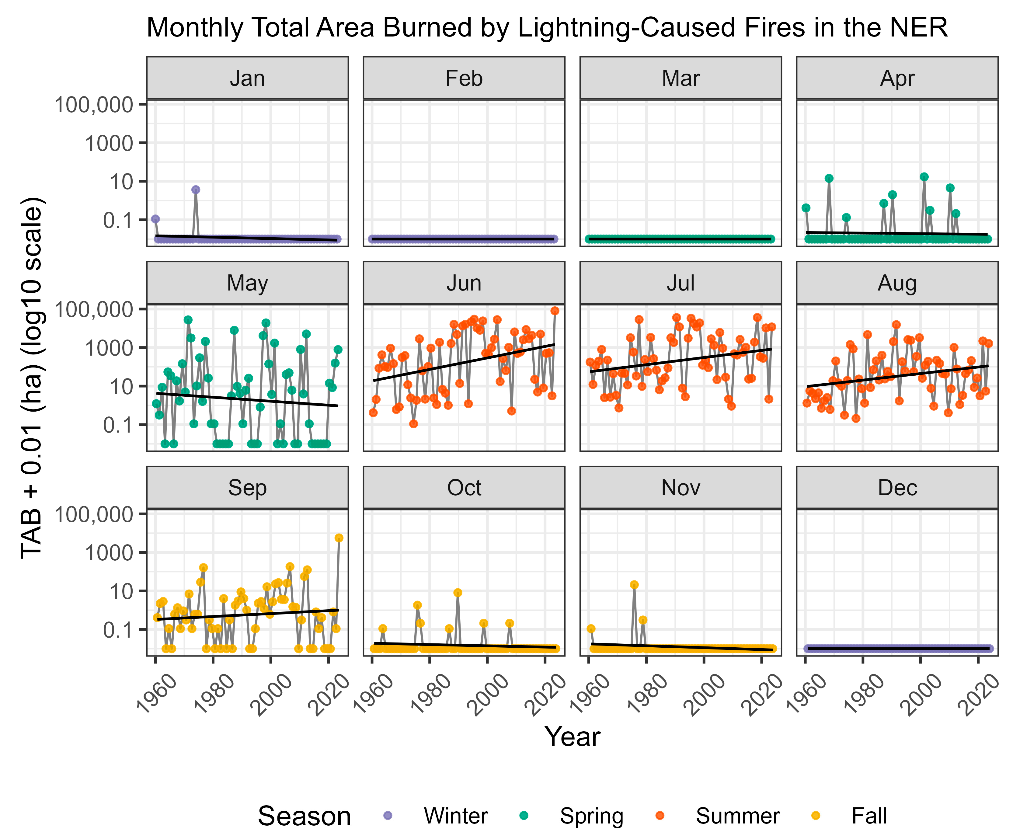
To accompany our analysis of monthly counts, we also consider the monthly total area burned (TAB) of both the ignition types in both regions. Figure 4 shows the TAB for human-caused fires in the NWR. Due to the wide range of observed values, we use a log10 scale to improve readability, as well as a small increase in the TAB of 0.01 ha (10% of the smallest positive observed fire size of 0.1 ha), so that months with zero TAB are not mapped to negative infinity. Note that this transformation and increase are used solely in these visualizations and not in any analysis. These agree with the count plots in Figure 3, with the winter months consistently having low TAB and approximately flat fitted trends, while the spring months (March–May) exhibit increasing variability and higher TAB values. TAB plots for human-caused fires in the NER, as well as lightning-caused fires in the NWR and NER, are included as Figure A4, Figure A5 and Figure A6 in Appendix A.2.
Figure 4.
Monthly total area burned (TAB) of human-caused fires in the Northwest Region (NWR) of Ontario. Approximate linear trends are illustrated as black lines.
The overall monotonic trend of the TAB and fire counts over the observed period is illustrated as black linear trend lines in each facet. Note that these are purely illustrative and are calculated during the plotting process, differing from estimates made by the CO method (especially for TAB, whose plots are on a log scale). Different months and causes have different visual distributions of points and fitted trend lines, with some panels exhibiting more obvious slopes, while others show comparatively flat trends. The late spring and summer months (June–August) account for the highest counts and TAB values overall, and the approximate trend lines also imply the possible existence of decreasing trends in counts and/or TAB from non-municipal human-caused fires ignited during the summer months in the NWR below 54° N. Our goal now becomes determining which of these trends are statistically significant.
3.3. Historical Trend Analysis
To begin our trend analysis, we examine the potential for autocorrelation in monthly fire counts from year to year using the DW test. Results indicate that fire counts for a given month are largely uncorrelated from one year to the next, with a few exceptions. The autocorrelation for human-caused fires in the NWR has a p-value below 0.05 in July (0.0276) and an approximate value of 0.2534. A positive autocorrelation suggests that years with high fire counts in July tend to follow each other (similarly for years with low counts). In the NER, human-caused fires also exhibited a significant autocorrelation value of 0.357 for August with a p-value of 0.0020. For lightning-caused fires in the NWR, June had a significant autocorrelation value of 0.3530 with a corresponding p-value of 0.0029, but no significant autocorrelations were found in the NER. While we do not conclude that there is substantial autocorrelation within monthly counts year-over-year, the few significant positive autocorrelations identified are in the important summer months. For this reason, we are motivated to use the CO method because of its ability to adjust for these autocorrelations and avoid an inflated rate of Type I Error. The results of applying the CO method to monthly counts are presented in Table 2, while some accompanying results for trends in TAB are in Table 3. Equivalent tests applied to annual total counts and TAB are also included, for both the working dataset and the datasets without filtering the municipal fires, to investigate the sensitivity of our results on the omission of those municipal fires.
Table 2.
Results of the Cochrane–Orcutt method investigating monotonic trends in the total counts of human- and lightning-caused fires per month, year-over-year, in both the Northwest and Northeast Regions (NWR and NER). Trends in the annual totals are also presented for the filtered dataset (Total 1) as well as the one including the municipal fires (Total 2). Statistically significant trends (p-value < 0.05) are emphasized using bold numbers.
Table 3.
Results of the Cochrane–Orcutt method investigating monotonic trends in the total area burned (TAB) of human- and lightning-caused fires per month, year-over-year, in both the Northwest and Northeast Regions (NWR and NER). Trends in the annual totals are also presented for the filtered dataset (Total 1) as well as one including the municipal fires (Total 2). Statistically significant trends (p-value < 0.05) are emphasized using bold numbers.
The results of the analysis in Table 2 identify some significant year-to-year monthly trends in monthly counts that are in alignment with Figure 3, Figure A1, Figure A2 and Figure A3. For lightning-caused fires, there are generally positive estimated trends during the summer, but they are not statistically significant. However, for human-caused fire counts, significant negative trends were observed in the summer months of June and July in the NWR, and May through July in the NER. In the NWR, significant negative trends are also observed for October and November, while there is a significant positive trend in March. Trends in annual totals are in alignment, with significant negative trends in human-caused fire counts and non-significant positive trends for lightning-caused fire counts. If we reintroduce municipal fires into this part of the analysis, we observe large changes in the human-caused fire count trends, with the trend approximately doubling in the NWR and increasing by a factor of six in the NER.
For trends in TAB presented in Table 3, most monthly trends were not statistically significant for either ignition type or region, apart from an increasing trend in TAB by lightning-caused fires in the NER in June of 193.8545 ha per year, with a p-value of 0.0414. All other months for lightning-caused fires in both regions exhibited no statistically significant trends, despite some large, estimated coefficients, particularly in the NWR during the summer months (e.g., 769.2752 ha/yr in July). In contrast to Table 2, while there are some negative trends in the TAB caused by human-ignited fires, these trends are not deemed statistically significant. Additionally, the estimated trend for May in the NER is positive, but similarly not significant. Annual total trends align with the monthly results, being negative for human-caused fire TAB in the NWR and positive in the NER (largely due to May), with both not significant. The estimated trend for annual TAB by lightning-caused fires in the NWR is large, but ultimately, we are unable to declare it significant due to the high level of variability in the underlying data. However, there is weak evidence in support of a moderately large increasing trend in the NER, having a p-value between 0.05 and 0.1, which is driven primarily by the observed trend in June. The impact of re-introducing the municipal fires is small on the annual total TAB trends of lightning-caused fires, as well as for human-caused fires in the NWR. The percentage change in magnitude for the positive trend in TAB by human-caused fires in the NER is larger, but this is largely a result of the original trend being relatively close to zero, in contrast to the others.
3.4. NB-AR Model Selection
We are interested in using an NB time series model to forecast future monthly fire counts. Models are fit separately for human- and lightning-caused fires within both regions, NWR and NER. Through our forecasting models, we aim to investigate the benefit of including one or more TCs as predictors (AMO, AO, ENSO, NAO, and/or PDO), both to improve model accuracy and to gain insight into whether these TCs have predictive skill at forecasting monthly fire counts in Ontario. Large-scale climate teleconnections, including the PDO, AO, AMO, and ENSO, are known to influence North American climate conditions. ENSO, for example, frequently peaks during boreal winter, and its downstream impacts on precipitation, drought, and fire–weather conditions can persist into the subsequent seasons [75,76,77,78,79,80]. These TCs naturally have temporal lags between the times of observing anomalies and when the influences of these anomalies are felt across different regions of North America, and the use of lagged predictors in the building of fire forecasting models is also supported by studies such as Dixon et al. [81], which have shown significant correlations between these indices and fire activity. We consider their inclusions at possible lags ranging from 1 to 12 months prior to the month we are forecasting for.
As observed in Figure 3, Figure A1, Figure A2 and Figure A3, there are certain months each year that rarely (if ever) observe fires from one or both sources, causing a strong deterministic seasonality that negatively impacted the model fits in our initial analyses. For instance, the inclusion of months like December and January in our models weakened their ability to detect a signal between the TCs and monthly fire counts, given that those months nearly always observed counts of 0 regardless of the lagged TC values. Accordingly, the decision is made to restrict our time series modeling to the months when fires tend to ignite, removing such months that had zero counts across most or all years. This represents different ranges of months for human- and lightning-caused fires based on their different seasonal ignition patterns. For human-caused fires, the modeling period included March through November, while for lightning-caused fires, we used April through October. Note that a limitation of this approach is that it assumes, in the human-caused models, for example, that the dependency between March and the previous year’s November is equivalent to the dependency between April and March. This discrepancy is minor at small lags, since months with small counts (February) are replaced by other months with small counts (November), but we are cautious of the impact of this choice at higher lags.
The dataset was split into a training period (1960–2010; 51 years) used for model fitting and a testing period (2011–2023; 13 years) for forecasting evaluation, relating to an approximate 80:20 split of our available data. All model selections were performed exclusively using the training period’s data. Prior to modeling, the autocorrelation structures in the raw fire counts are investigated using the autocorrelation function (ACF) and partial autocorrelation (PACF) plots, as seen in Figure 5. Both human- and lightning-caused fires exhibit a repeating correlation structure that is aligned with the lengths of their shortened years, nine months for human-caused fires and seven months for lightning-caused fires. Conversely, a cutoff in the significant lags in the PACF terms occurred at a lag of 9 months (with only one or two minorly significant terms at later lags in some cases). These results together indicate that the underlying structure is approximately that of an AR(9) framework, implying that our models do not have a need for any MA terms. Relative to the general model in Equation (4), we therefore drop all MA terms and include AR terms for up to lag 9. The simplified form our models take is therefore
where we have yet to define the predictors .
Figure 5.
Autocorrelation function (ACF) and partial autocorrelation function (PACF) plots of raw counts and residuals from the considered NB-AR models. Columns denote a combination of the fire cause (H for human, L for lightning) as well as the region (NWR or NER). Autocorrelations and partial autocorrelations that fall within the dashed red lines are not statistically significant.
From our fire counts’ ACF plots, we note that the repeating pattern is naturally seasonal in nature. We incorporate this seasonality into the models by introducing monthly indicator variables to adjust the means of the processes each month relative to a baseline. These indicators are defined as follows:
For human-caused fire models, the base case is the month of March, so we introduce indicator predictors for months 4 (April) through 11 (November). Similarly, for the lightning-caused fire models, April is the base case, and there are indicators for months 5 (May) through 10 (October). Henceforth, we refer to these seasonal models lacking any TC predictors as our “Null” models. In Figure 5, we can see that these Null models capture most of the underlying temporal dependencies, leaving us with residuals that are largely uncorrelated other than a few significant ACF and PACF spikes in some but not all models. Overall, the human-caused Null models appear to fit the data slightly better than the lightning-caused Null models.
To potentially improve the model fit beyond that of the Null models, we now consider a series of “TC” models that allow for the addition of teleconnections as linear predictors alongside the AR(9) structure and seasonal monthly indicators. Each of the five TC anomaly variables can either be absent or included with a lag of 1 to 12 months, resulting in 135 = 371,293 potential models for each of the four cause–region combinations. Each model is fit using just the training data ending in 2010 and its specific combination of lagged TCs. For each case, the model with the smallest AIC is selected. Hence, with the goal of prediction, we are prioritizing overall model fit, as measured by AIC, which can result in the inclusion of multiple predictors having non-statistically significant coefficients. If the primary goal were to make historical inferential claims and identify only significant terms, then an alternative iterative model selection approach would be more appropriate (e.g., backwards selection). A summary of the lag combinations of these selected TC models, their AICs, and their respective null models’ AICs (for reference) is summarized in Table 4.
Table 4.
Selected teleconnection (TC) models’ variable lags for human- and lightning-caused models for the Northwest Region (NWR) and Northeast Region (NER). Dashes indicate predictor variables omitted from the selected models. AIC values of the TC models are provided along with the corresponding AIC values of their respective Null models that are fit without any TC variables.
For the human-caused TC models, the improvement in AIC for the NWR is modest (3143.144 vs. 3160.406), while a larger improvement is found for the NER model (3055.775 vs. 3103.114). These models use five and four TC variables, respectively, and we observe a commonality in their dependence on 12-month lagged AMO. The lightning-caused TC models, both using four TC variables, experienced large or respectable improvements in AIC (2711.994 vs. 2874.305 for NWR; 2194.823 vs. 2246.242 for NER). ACF and PACF plots of the TC model residuals are presented in Figure 5. For HNWR (i.e., human-caused fire model for the NWR), there were no significant spikes in either plot, which remains the case. For the similarly named HNER and LNWR, some but not all significant PACF spikes now fall within the dashed lines, indicating that they are no longer statistically significant, and so the TC model better captures the temporal correlations in the data. Lastly, for LNER, the two significant spikes in both plots now fall within the dashed lines, which importantly includes the spikes at lag 1.
Our selected TC models’ coefficients and corresponding lower and upper confidence intervals are presented in Table 5. Any coefficient whose interval does not cover 0 is deemed statistically significant at a 5% significance level, so those terms are emphasized using bold font. From this table, we note that the only statistically significant AR term corresponds to the 1-month-lagged observations, while all but the latest months’ indicators are significant. The positive coefficients indicate that months with large counts are more likely to be followed by months with large counts, while the significant positive coefficients on most month terms relate to the increase in average fire occurrence in those months relative to their model’s base cases which observe only a few or no fires in a typical year (March for human-cause, April for lightning-caused). With respect to the TC variables themselves, we find that 12-month-lagged AMO anomalies are significant in the human NER model, but despite having a larger absolute magnitude than the other TC predictors’ coefficients, they just fail to be significant in the NWR model. However, we note that these 12-month-lagged AMO values do become significant in the NWR models for some alternative cutoffs (e.g., if we fit the model using data up through to the end of 2017 instead of 2010). For the lightning models, we find that a 7-month-lagged AO anomaly is significant for NER, while no TC terms come out as significant in the NWR model.
Table 5.
Estimated coefficients ( or ) and 95% confidence interval lower bounds (L.B.) and upper bounds (U.B.) for the selected NB-AR “TC” models for human- and lightning-caused monthly fire counts in Ontario’s Northwest Region (NWR) or Northeast Region (NER).
3.5. Investigating Predictive Skill Through Cross-Validation
The models described in Table 4 and Table 5 were fit using the training data that only goes to the end of 2010. To investigate how these models would perform at forecasting future values, we use the testing data for the years 2011–2023. We consider two forecasting scenarios: forecasting one month ahead of the present (“1-month-out” forecasts), or forecasting the summer months at the end of the first month of the operational fire season, April (“from April” forecasts). For the sake of these cross-validations, we consider the reasonable scenario where such a model would be updated with current data before making any forecast. So, while the chosen predictors do not vary between forecasting scenarios, the data used to fit the models gradually increase either one month at a time (for one-month-out forecasts) or one year at a time (for summer forecasts from April). We note that for all forecasts, for simplicity, accurate historical TC anomaly values are used, even if they would not be available in practice for some of the forecasts made from April. For example, the NWR TC model for human-caused fires relies on a two-month lagged ENSO anomaly, which would not be available in April when forecasting for August (since it would be June’s value). In practice, if forecasts at large temporal leads are desired, alternative models that only rely on larger lags can be considered for use in place of these TC models that absolutely minimize AIC, which should result in similar, but likely slightly worse, performance. This is not a concern for the one-month-out forecasts, however.
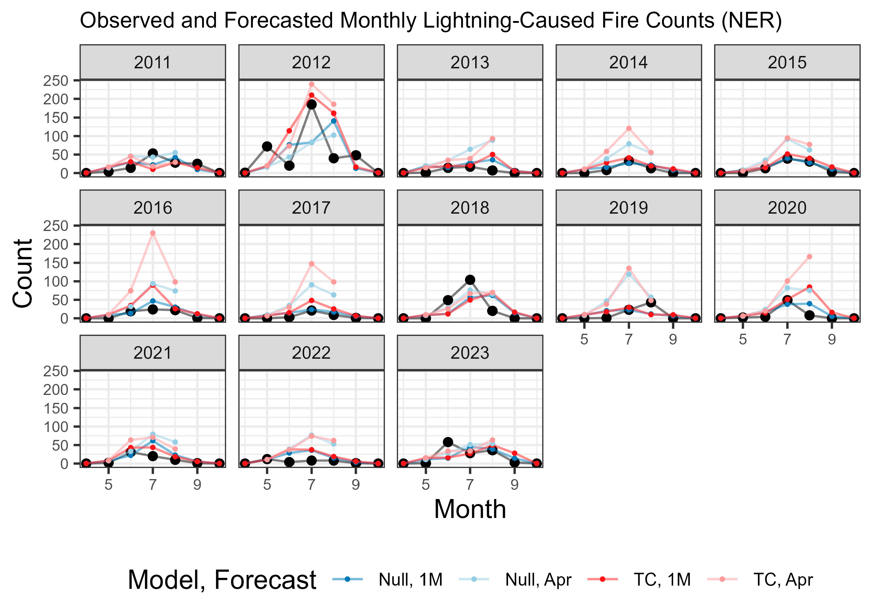
Forecasted values are compared against raw counts in Figure 6, Figure A7, Figure A8 and Figure A9 in Appendix A.3. As one would expect, the forecasts made further into the future more closely resemble the historical averages, while the one-month-out forecasts are able to more dynamically adapt as a fire season goes on. The precision of these forecasts is higher for the human-caused models, given that their largest forecasted means are generally smaller than those of the lightning-caused models, and as noted in Equation (3), the variance of the NB distribution is an increasing function of its mean. To quantitatively summarize and contrast the cross-validated forecasting accuracies, we consider the Mean Absolute Errors (MAEs) for the peak summer months (June, July, August), defined as the average absolute value of the difference between the forecasted mean count and the actual observed number of fires for a given month. Alongside the MAE values for the TC and Null models, we also consider the percent change in MAE relative to the Null models:
These MAE and percent change in MAE values are presented in Table 6. If a TC model were on average more accurate, then ; in this case, we observe a positive percent change equivalent to the percent reduction in MAE relative to the Null model. However, if a TC model performed worse, this percent change is negative, relating to the percent increase in MAE (i.e., for the lightning-caused NER models).
Figure 6.
NB-AR Null and TC model forecasts on the testing data of monthly human-caused ignitions from 2011 to 2023 in the Northwest Region (NWR) of Ontario. Historical counts are illustrated with black dots/lines. Forecasts are either one-month-out (“1M”) or simultaneously performed for the months of May through August from the end of April (“Apr”).
Table 6.
Mean Absolute Error (MAE) comparisons between TC and Null models for human- and lightning-caused fire count forecasts across the Northwest Region (NWR) and Northeast Region (NER) at 1-month-out and April forecasts. Positive percentage changes relate to improvements (lower error) by the TC model relative to the Null model. Considered months’ forecasts are June, July, and August between the years of 2011 and 2023.
For human-caused fire counts, the two TC models show a respectable reduction in average forecasting error relative to their respective Null models. The percent reduction in MAE for the rolling 1-month-out forecasts ranges between 13% and 18%, while larger percent reductions are evident in forecasts made multiple months out from April, with the highest improvement seen for the NER April forecast, where the TC model reduces the error by nearly a third compared to the Null model. However, for the lightning-caused fire counts, the average performances of the TC models are mixed. In the NER, the TC model slightly underperforms relative to its Null model, with MAE increasing by about 9.8% for 1-month forecasts and 17.2% for April forecasts. Comparatively, for the NWR, we observe similar improvements in the one-month-out forecasting accuracy as seen in the human models (16.7%), but a smaller gain in those made at the end of April (8.6%).
Comparing the magnitudes of the MAEs between the lightning and human models, we see a stark difference, with MAEs being larger when forecasting lightning fire counts. This is driven, in part, by some bad fire seasons such as 2021 in the NWR that observes some forecasting errors in the hundreds (underestimation in June and July, followed by an overcorrection in August). Furthermore, for the April forecasts, since most April months observe few to no lightning fires, the forecasts for the upcoming fire seasons use similar data each year, despite lightning counts having a higher natural variability, with differences in predictors primarily coming from previous year’s fires (which have a weaker relationship), and in the TC models, the lagged teleconnections. In the aggregate, there is less of a clear picture as to the predictive skill of TCs in the lightning-caused fire models, with higher variances in forecasting errors resulting in more uncertainty in the precision of our MAE values as estimates of the true difference in average forecasting error, but the mixed results that, in our opinion, suggest that it would be worth further investigation.
4. Discussion
Our time series analyses are divided into two main parts. First, we applied the Cochrane–Orcutt (CO) method to evaluate and test for historical trends in counts of human- and lightning-caused fires during different months in the Northwest and Northeast Regions (NWR and NER) of Ontario, Canada. Prior to running these tests, we used the Dubin–Watson (DW) test to assess temporal autocorrelations in monthly values across successive years. Significant positive autocorrelation was detected in some key summer months, justifying the need for the CO method to avoid inflated Type I Error probabilities.
The results of the CO method presented in Table 2 display significant negative trends in the number of human-caused fires in both the NWR and NER. This may be reflecting the effectiveness of fire prevention strategies targeting human-caused ignitions, such as increased public education and tighter land-use regulations implemented across Ontario in recent decades [56]. Our results are consistent with findings from other studies conducted in Canada, which have reported a decrease in human-caused fire occurrence due to enhanced fire management and public compliance with fire bans [29,30,57]. Some other factors that help reduce or avoid increases in the occurrence of human-caused fires in Ontario include FireSmart [82] and legislation such as the Modifying Industrial Operations Protocol (MIOP), which has been shown to be successful, relative to previous regulations, at avoiding increases in the probability of igniting fires from forest industry operations [83] while also helping reduce the amount that a fire ignited by forest industry operations grows after detection [84]. These negative trends contradict the forecasts of Wotton, Martell, and Logan [56] who predicted human-caused fires to increase, but as they remarked, such predictions are dependent on potential changes to land use, education, and government policy, which were not captured in their model. That said, we also detected an increasing, albeit weak, trend in the NWR for the month of March, which may be some evidence of the human-caused fire season being more active earlier in the year.
In contrast, counts of lightning-caused wildfires in the NWR and NER have no significant trends. This outcome of the CO method agrees with the visual trends (or lack thereof) from Figure A2 and Figure A3. An absence in decreasing trends relative to the human counts is not surprising, given that lightning ignitions are primarily driven by atmospheric conditions [30], so their frequencies are related to climate drivers rather than human regulations. Thus, prevention efforts such as education campaigns do not have a direct impact on their frequency. We do note that the single highest estimated trend, an increase of 1.0097 lightning-caused fires per year in the month of July, is in the NWR. The p-value of 0.2578, not being small enough to declare the trend significant, is a consequence of more natural variability in lightning-caused fire counts, making it more difficult to detect the signal from the noise. So, it may be the case that the number of lightning-caused ignitions is increasing in some months, but we would require more years of data to formally draw that conclusion.
To accompany these results and obtain a more complete picture of the impact of climate change in Ontario, the CO method was also used to investigate trends in the total area burned (TAB), as presented in Table 3. There were no significant trends in monthly TAB for human-caused fires, although the summer months still exhibited negative trends. The lack of significance, despite our evidence of decreasing counts, is likely due to higher relative variability in TAB values versus counts, while using the same number of data points in the tests. However, we do detect a significantly increasing trend in lightning-caused TAB for the NER in June. There are some even larger estimated trends in NWR, but the data are too noisy to declare them significant. Thus, although the statistical evidence is modest, we are still able to conclude that there has been some increase in the area burned by lightning-caused fires in Ontario.
As a quick sensitivity analysis, trends in annual total counts and TAB were investigated using our filtered dataset of 51,155 fires, as well as a larger one that did not omit municipal areas that contain information on 88,573 fires. The additional data results in larger annual count and TAB values, but no more observations are used in the CO method, since all values are aggregated yearly. The inclusion or exclusion of the municipal fires do not change any major conclusions, although there are notable changes in the estimated trends in annual total counts of human-caused fires, especially in the NER, where the negative trend increased by a factor of six, although this may be amplified somewhat from a negative bias stemming from underreporting as a consequence of Municipal Protection Areas (MPAs). That said, this trend experiencing the largest change is not unexpected, given its dependency on the subset of the data that experienced the greatest reduction because of the municipal area filter (36,119 to 9968). This motivates a possible reproduction of this or a similar study in the future, should historical MPA records be digitized and made available.
The second part of our analysis involved developing Negative Binomial Autoregressive (NB-AR) models to forecast future months’ counts of human- or lightning-caused fires in the NWR and NER. After determining that an AR(9) framework was reasonable for the base of the models (Figure 4), average seasonality was modeled using month indicator functions as defined in Equation (6), and teleconnections (TCs) were incorporated to possibly further improve model fit while enabling our side goal of an investigation into whether these variables exhibit predictive skill in counts of ignitions across Ontario.
Our model selection considered 135 = 371,293 candidate models for each cause–region combination that considered each of our five TC variables at lags between 1 and 12 months (or had them omitted entirely). The selection procedure was conducted on training data spanning years 1960 through 2010 and chose the respective models that minimized AIC, favoring overall goodness of fit versus individual coefficient significance. The optimal TC lags are presented in Table 4, while the coefficients and their 95% confidence intervals are found in Table 5. The only significant TC coefficients were for AMO at a 12-month lag in the human NER model, as well as AO at a 7-month lag in the lightning NER model. However, as noted earlier, AMO does become a significant predictor in the NWR when a different cutoff is used in the data, so further investigation into the connection between AMO and human-caused ignitions in Ontario may be warranted as future work.
The consistent inclusion of AMO at about a year’s lag that we found in optimal models supports its long-term influence on fire activity, potentially by affecting drought, temperature, and moisture that shape seasonal fire ignitions. However, the negative relationship between AMO and human-caused fire counts corresponds to fewer ignitions. While a positive AMO phase is generally associated with hotter and drier conditions in parts of Eastern Canada [17,85], increased awareness and institutional readiness during such periods may lead to enhanced prevention measures, education campaigns, and enforcement, thereby reducing the number of ignitions [29,30,57,86], even if the potential hazard of fires that ignite during those periods is higher. Physically, negative AMO phases are often associated with cooler conditions and, in many regions in eastern North America, neutral to higher precipitation and wetter soils [87]. While these conditions reduce climatic fire occurrence, human activity, land-use patterns, and institutional feedback can still influence the likelihood of human-caused fires. Conversely, although not statistically significant, the lagged AMO term in the lightning-caused NER model had a positive coefficient, which would align with the typical expectation that hotter and drier conditions can lead to an increase in lightning-caused ignitions. These findings highlight the indirect influence on AMO variability in fire occurrence from different sources, emphasizing the importance of considering both climate variability and socio-institutional controls in interpreting the observed trends.
The coefficient on lagged AO in the lightning-caused NER model was positive. Positive AO conditions are characterized by stronger winds and low sea-level pressures over the polar region, which leads to warmer and unstable atmospheric conditions over northeastern North America [88]. These conditions increase convective activity and increase lightning frequency, which can directly cause the likelihood of lightning-caused fires. Hence, a positive AO coefficient for the lightning-caused fires reflects a direct atmospheric ignition potential.
Other significant model coefficients include most of the seasonal month indicators as well as , the coefficient of (the previous month’s count). The other AR terms are not significant at the level 0.05 in the presence of the month indicators. Given that we trimmed and stitched our time series to remove months that deterministically observed counts of zero, caution would be warranted when considering the importance of higher-order lagged terms. However, our models’ emphasis on the impact of the AR(1) term over the others at higher lags mitigates the potential errors that could be incurred from this approach, reassuring us in the appropriateness of our final TC models.
The predictive skill of the TC models (with teleconnections) was compared against their respective Null models (without teleconnections) through a cross-validation study on the testing data between 2011 and 2023. Performance in the summer months of June through August was highlighted, and two types of forecasts were considered: rolling one-month-out forecasts, or the forecasting of the summer months all at once from the month of April. MAE values for the TC and Null models, as well as the relative percent change in MAE by a TC model versus its corresponding Null model, are presented in Table 6.
Our findings show that the use of teleconnections in predictive modeling in Ontario has promise. For both human-caused fire count models, there was a respectable decrease in MAE observed by the TC models, with one-month-out forecasts seeing a relative improvement of 13.8% (NWR) and 17.4% (NER), while forecasts made from April observed larger improvements of 21.2% (NWR) and 29.8% (NER). Conversely, the relative performances for the lightning models were mixed. In the NWR, we observed relative decreases in MAE of 16.7% (one-month-out) and 8.6% (from April), but MAE increased by 9.8% (one-month-out) and 17.2% (from April) for the NER.
With this in mind, we emphasize the relative differences in the MAE values themselves, which are much smaller for counts of human-caused fires than for those ignited by lightning. This follows at least partially from lightning counts during summer months having larger means (Figure 2). As mentioned in Equation (3), the variance of a negative binomial distribution, and hence the spread of values around its mean, increases with the mean. Accordingly, there is more uncertainty when predicting larger values, leading to larger absolute errors more often. A consequence of this is that the use of these cross-validated MAE values as estimates of the true expected absolute errors of these models has more uncertainty in the lightning-caused models than the human-caused models, given the same amount of data points (months) used in their fitting, which should be taken into consideration when interpreting their values and making a conclusion about whether the TCs help the forecasts or not (or by how much). Larger variance aside, it is also the case that since lightning ignitions are related to short-term convective weather processes, large-scale climate indices such as TCs may in fact have limited predictive skill. This would align with earlier studies that found a weak or inconsistent relationship between teleconnections and lightning-caused fire activity [30,89,90].
Another consideration for the lightning-caused models (Null or TC) is that the further-out forecasts are being made from April, which typically observes a count of zero or near-zero. As a result, the “from April” forecasts tend to be closer to historical averages if they regularly begin with a one-month-lagged value of 0 (the most important autoregressive term, according to Table 5). An argument could be made to instead delay a month and make lightning-ignited fire forecasts after May, which would likely reduce the MAEs of these forecasts to something closer to the one-month-out forecasts’ MAEs.
We close the Discussion by acknowledging a limitation in our study. Namely, the omission of fires ignited within known Municipal Protection Areas (MPAs) (Figure 1) as well as other municipal areas that may have been MPAs in the past. This decision avoided potential biases that could have been introduced into the trend analysis and forecasting due to changes in the reporting and recording of fire data. These potential biases may partially explain the large difference in the estimated trend for the total annual count of human-caused fires in the NER when omitting or including municipal fires (Table 2). However, it did have the undesirable result of removing a large amount of data and restricting our analyses to areas of land away from the wildland–urban interface (WUI), so our conclusions should be interpreted in terms of our official study region, that is, non-municipal areas of Ontario below 54° N. If a future study were interested in trends and forecasting in the WUI in Ontario, historical records on where and when the MPAs were in effect would be required to obtain unbiased results.
5. Conclusions
This study investigated historical trends and the forecasting of monthly counts of fires ignited by humans or lightning across the Northwest and Northeast Regions of Ontario, Canada. Trend analyses made use of the Cochrane–Orcutt method to detect significant trends in monthly fire counts, as well as the total area burned, while accounting for potential temporal autocorrelations year-over-year. The method revealed a statistically significant decreasing trend in human-caused fires for many summer months, likely reflecting the effectiveness of ongoing fire prevention efforts, public education, and regulatory measures. In contrast, lightning-caused fires showed non-significant trends for counts, but there was some evidence of an increase in the total area burned (primarily during June in the NER). That said, given the large, estimated trend in July fires ignited by lightning in the NWR, it is likely that the larger amount of variation in lightning-caused fires is making it more difficult to declare significant the trends in lightning-ignited fire counts, which could change if this study is repeated in the future with more data.
In the literature, there have been established connections between lagged teleconnections and climate variables related to wildland fire. In addition to investigating trends, our other goal was to investigate how well we can forecast these counts, in addition to determining which TC’s, if any, can assist in improving our Negative Binomial Autoregressive time series model’s predictive skill (and at what lags). Our results found that a remarkable improvement in prediction accuracy was obtained in the models of human-caused fire counts incorporating AMO at a 12-month lag, relative to the equivalent Null model fit without the use of any TC predictors. However, the impact of using TCs in modeling lightning-caused fire counts was mixed. Accordingly, large-scale teleconnections may not significantly improve prediction for lightning-caused fire activity in our study region. This might be because of features of lightning-caused ignitions, such as a heavy reliance on localized weather events (i.e., lightning storms). This finding is in line with previous studies, which have also discovered weak correlations between climate teleconnections and lightning-caused fire occurrence.
Future forecasting efforts should prioritize customized models for different ignition sources that consider seasonal timing and regional climate drivers, as the risk of wildfires continues to increase due to climate change. Seasonal fire forecasts in the Northwest and Northeast Regions of Ontario and elsewhere could be made more accurate by utilizing more high-resolution weather data, adding fuel moisture conditions, and investigating additional regional or local predictors. Using smoothed functions of teleconnections rather than assuming a true linear relationship is also another avenue to improve the fit of these models. Developing more advanced models incorporating these features is a possible direction of future work in this area. Furthermore, it would also be of interest to investigate predictive models of the total area burnt or the final size of individual fires to study and quantify relationships between the fire size and teleconnections.
Author Contributions
Conceptualization: K.G. and E.B.; methodology: E.B. and K.G.; software: K.G. and E.B.; validation: K.G. and E.B.; formal analysis: E.B. and K.G.; investigation: E.B.; resources: K.G.; data curation: K.G. and E.B.; writing—original draft preparation: E.B.; writing—review and editing: K.G. and E.B.; visualization: K.G. and E.B.; supervision: K.G.; project administration: K.G.; funding acquisition: K.G. All authors have read and agreed to the published version of the manuscript.
Funding
This work is supported in part by funds from the Natural Science and Engineering Research Council of Canada (NSERC) through its Discovery Grant program (RGPIN-2024-03841).
Data Availability Statement
The MNR datasets used for our analyses are copyright the King’s Printer for Ontario, as represented by the Ontario Ministry of Natural Resources, and were used under license. The Canadian National Fire Database, while partially incomplete, is derived in part from this data and is publicly available through the CWFIS Datamart hosted by Natural Resources Canada [91]. Other datasets used from the Ontario GeoHub and NOAA [63,64,65,66,67,68,69] are publicly available.
Acknowledgments
We thank the Ontario Ministry of Natural Resources for providing access to their data used in our study. We also thank D. Boychuk from the MNR for contributing some helpful advice during the early stages of this project.
Conflicts of Interest
The authors declare no conflicts of interest.
Appendix A
Appendix A.1. The Cochrane–Orcutt Method
The CO method is used to adjust an ordinary linear regression model to accommodate a first-order serial correlation in its errors. This occurs when the error terms in the model correlate with the error terms in the preceding observations, often due to temporal dependence in the data. Note that CO assumes that the error terms follow an AR(1) process, which may not be suitable for all types of data [45,92].
Consider a regression model,
where is the dependent variable observed at times , N, is the intercept, is a vector of regression coefficients, is a vector of predictor variables at time , and is the error term of the model at time Suppose that temporal autocorrelation is present among the model error terms, and the residuals can be represented using a first-order autoregressive term as
where is the temporal autocorrelation coefficient between pairs of observations with , and is an independent white noise at time The CO method proceeds to adjust for the autocorrelation by taking a generalized differencing of each term in Equation (A1). This transformation is given as
where we recognize that By defining the transformed variables
Equation (A3) simplifies to the regression model
which can be analyzed using ordinary linear regression to obtain an unbiased estimate of . For our trend analysis, it suffices to let the vector be the scalar , in which case the scalar can be interpreted as the average linear trend. The test was implemented using code from the orcutt package in R. However, it must be noted that it has since been archived and is no longer accessible for the current version of R.
Appendix A.2. Monthly Time Series Plots
Here, we present additional monthly time series figures for human-caused fires in the NER (Figure A1), as well as lightning-caused fires in the NWR (Figure A2) and NER (Figure A3). Equivalent plots for monthly total area burned (TAB) are presented in Figure A4, Figure A5 and Figure A6.
Figure A1.
Monthly counts of human-caused fires in the Northeast Region (NER) of Ontario. Approximate linear trends are illustrated as black lines.
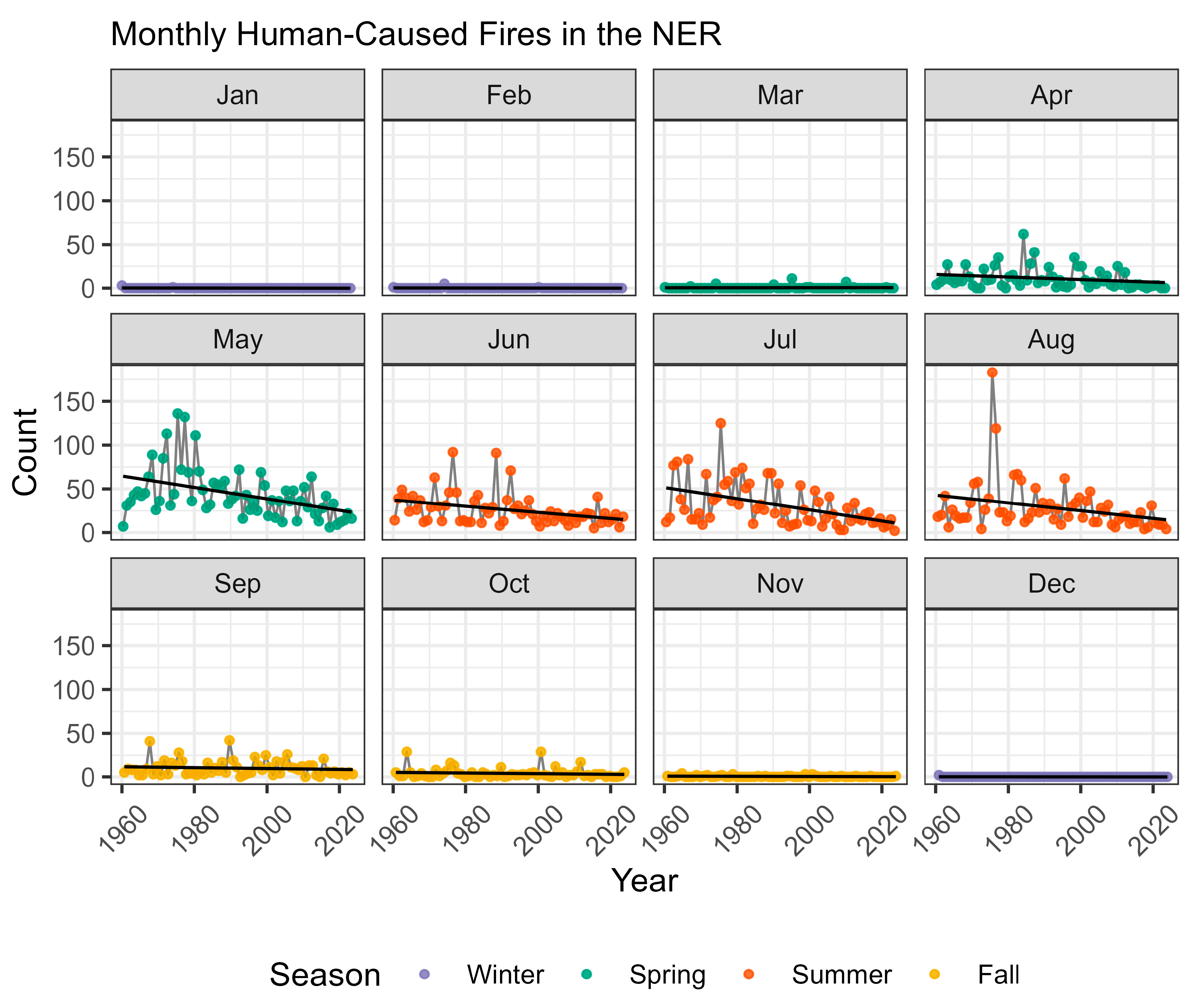
Figure A2.
Monthly counts of lightning-caused fires in the Northwest Region (NWR) of Ontario. Approximate linear trends are illustrated as black lines.
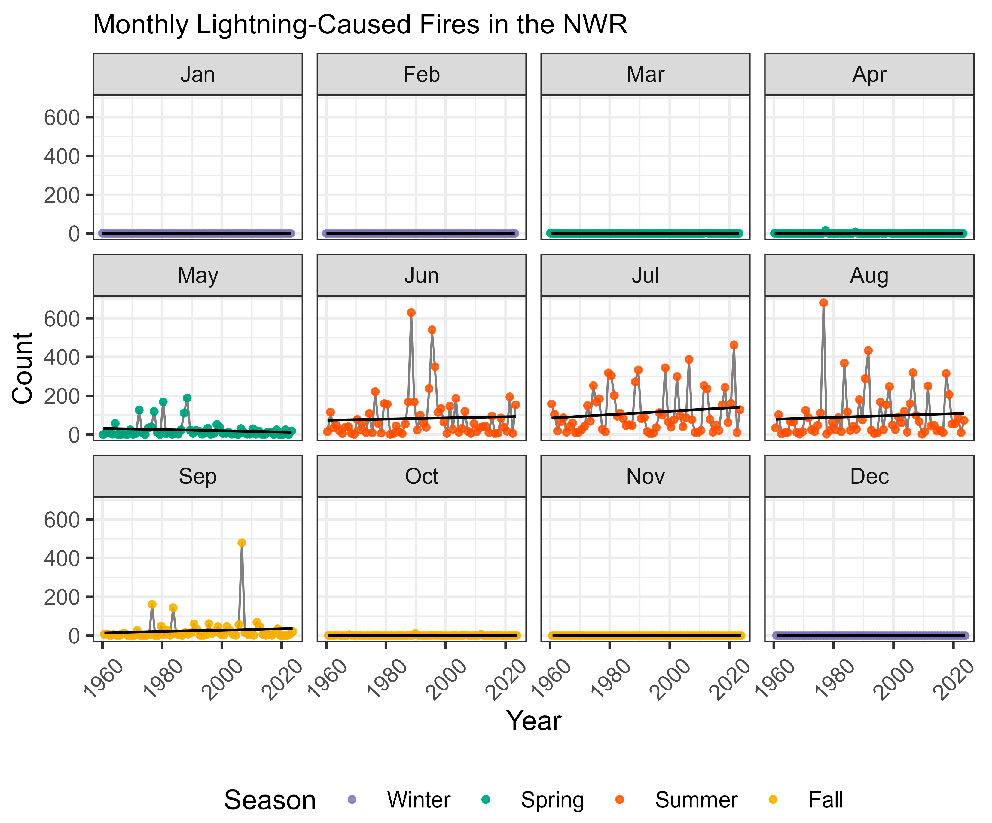
Figure A3.
Monthly counts of lightning-caused fires in the Northeast Region (NER) of Ontario. Approximate linear trends are illustrated as black lines.
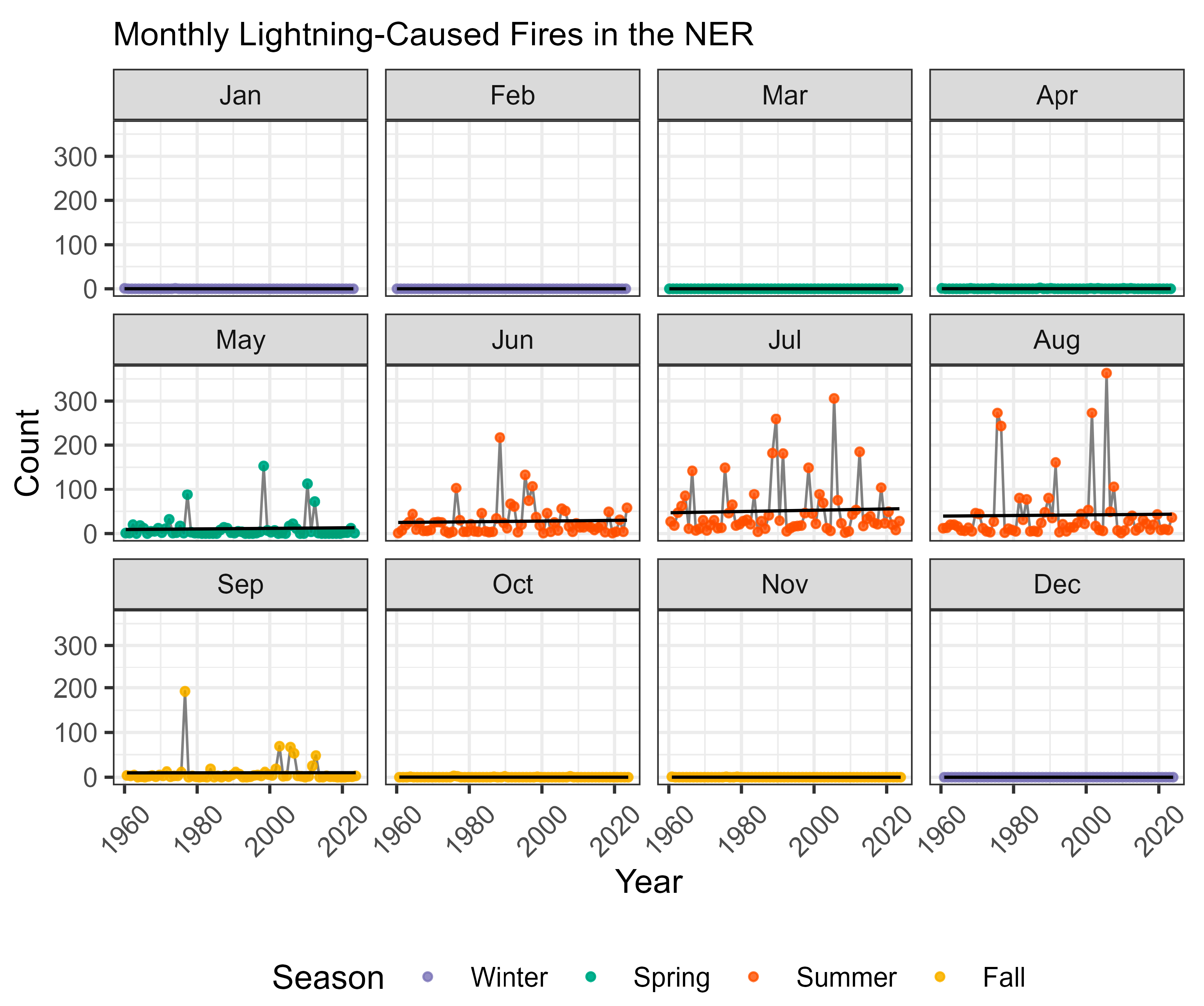
Figure A4.
Monthly total area burned of human-caused fires in the Northeast Region of Ontario. Approximate linear (monotonic) trends are illustrated as black lines.
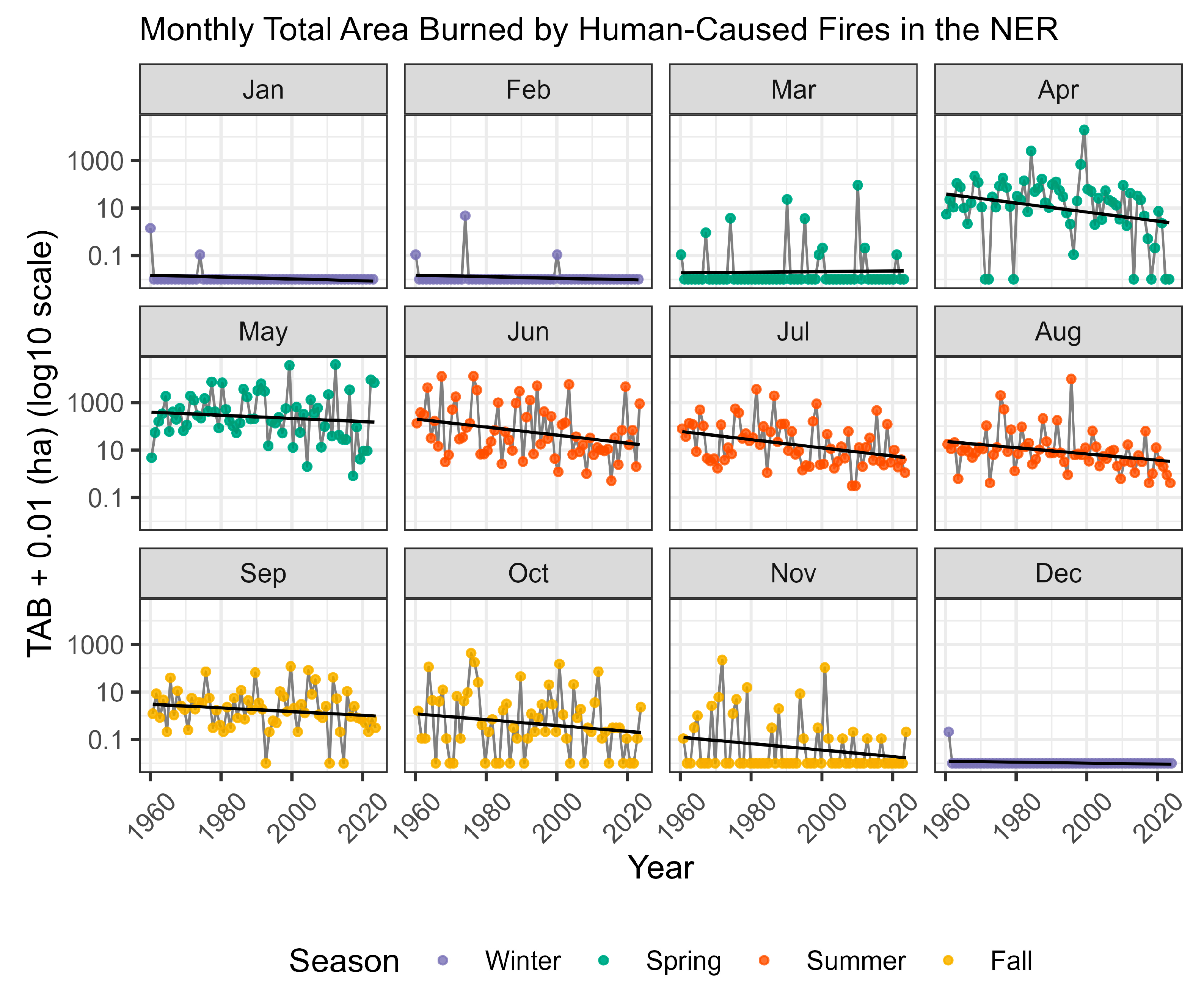
Figure A5.
Monthly total area burned of lightning-caused fires in the Northwest Region (NWR) of Ontario. Approximate linear trends are illustrated as black lines.
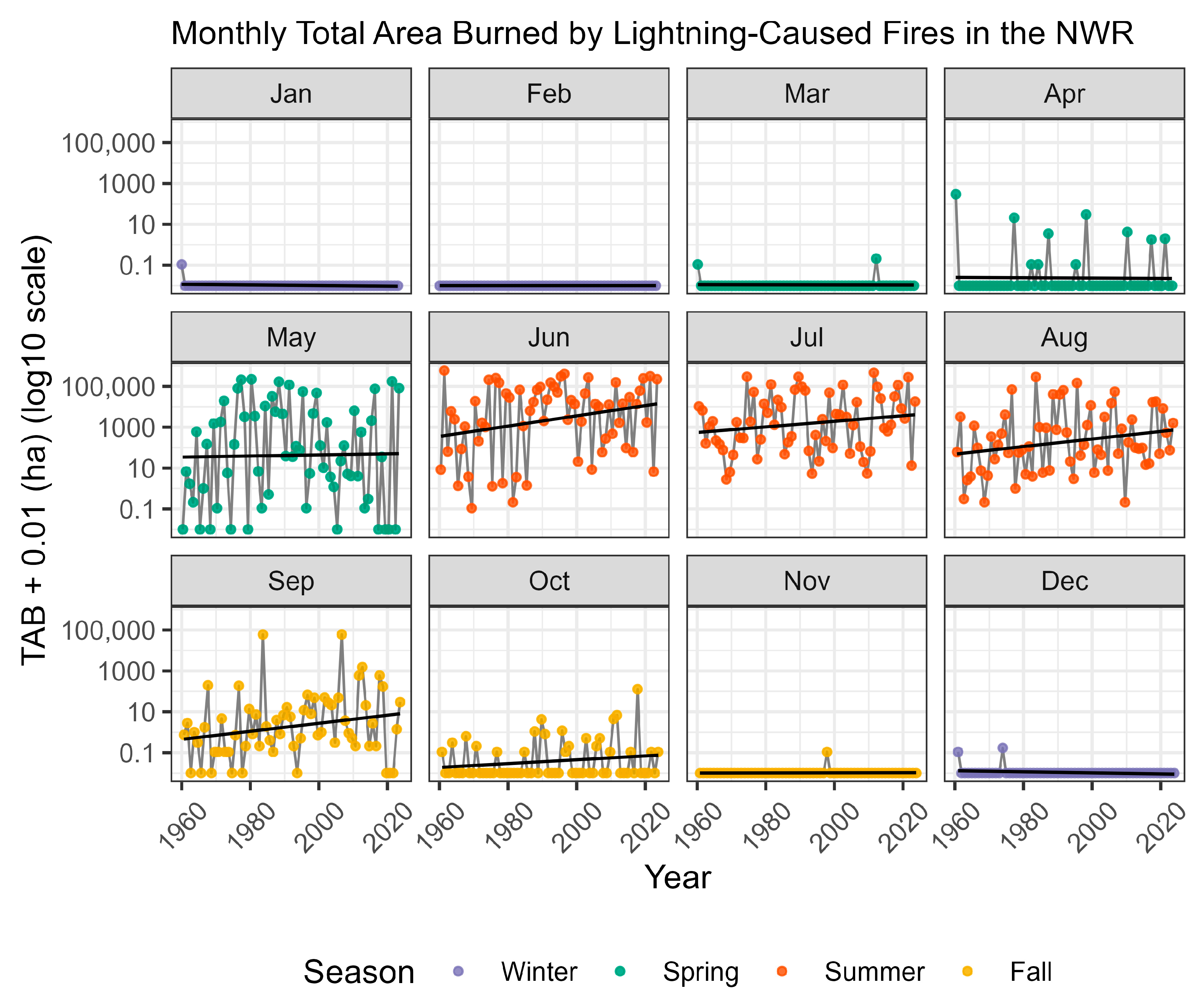
Figure A6.
Monthly total area burned of lightning-caused fires in the Northeast Region (NER) of Ontario. Approximate linear trends are illustrated as black lines.
Appendix A.3. Observed and Forecasted Monthly Fire Count Plots
Here, we present additional plots contrasting the observed counts and their forecasted values for the years 2011 through 2023 using our Null and TC NB-AR models. Human-caused fires in the NER are visualized in Figure A7, while lightning-caused fires in the NWR and NER are presented in Figure A8 and Figure A9, respectively.
Figure A7.
NB-AR Null and TC model forecasts on the testing data of monthly human-caused ignitions from 2011 to 2023 in the Northeast Region (NER) of Ontario. Historical counts are illustrated with black dots/lines. Forecasts are either one-month-out (“1M”) or simultaneously performed for the months of May through August from the end of April (“Apr”).
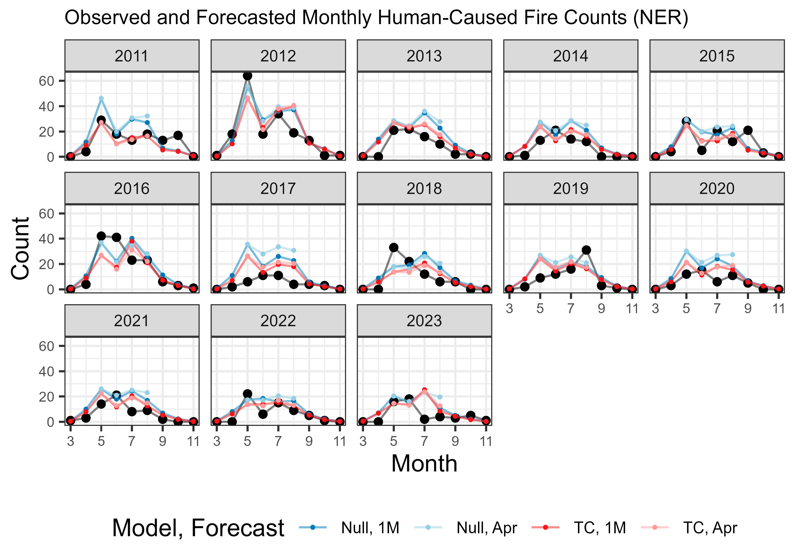
Figure A8.
NB-AR Null and TC model forecasts on the testing data of monthly lightning-caused ignitions from 2011 to 2023 in the Northwest Region (NWR) of Ontario. Historical counts are illustrated with black dots/lines. Forecasts are either one-month-out (“1M”) or simultaneously performed for the months of May through August from the end of April (“Apr”).
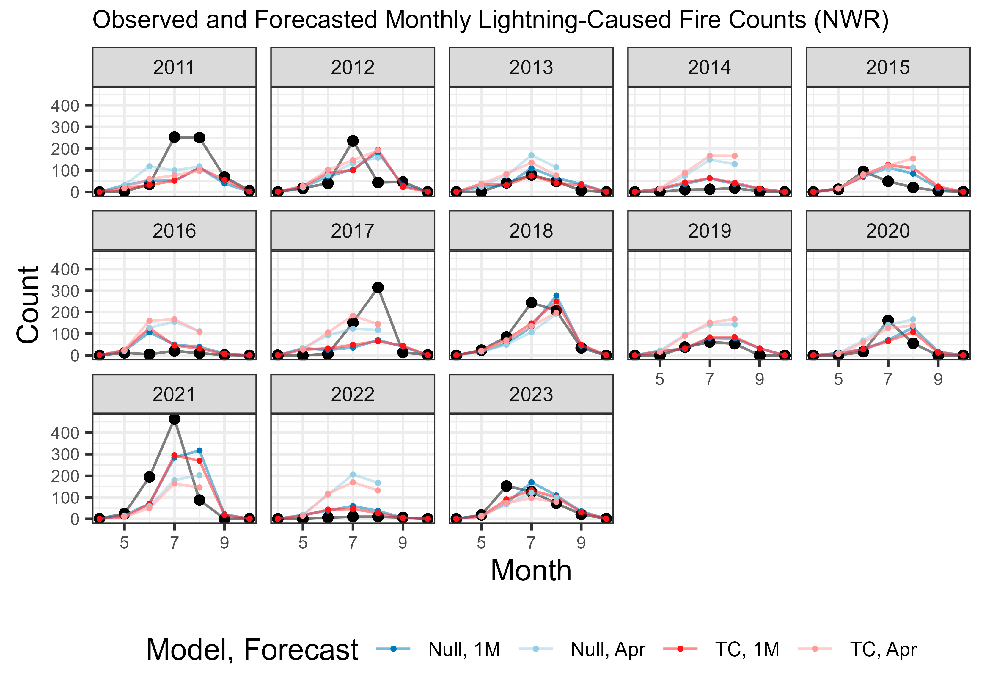
Figure A9.
NB-AR Null and TC model forecasts on the testing data of monthly lightning-caused ignitions from 2011 to 2023 in the Northeast Region (NER) of Ontario. Historical counts are illustrated with black dots/lines. Forecasts are either one-month-out (“1M”) or simultaneously performed for the months of May through August from the end of April (“Apr”).
References
- Weber, M.G.; Stocks, B.J. Forest Fires and Sustainability in the Boreal Forests of Canada. Ambio 1998, 27, 545–550. [Google Scholar]
- Pausas, J.G.; Keeley, J.E. Wildfires and Global Change. Front. Ecol. Environ. 2021, 19, 387–395. [Google Scholar] [CrossRef] [Scilit]
- Pausas, J.G.; Ribeiro, E. The Global Fire–Productivity Relationship. Glob. Ecol. Biogeogr. 2013, 22, 728–736. [Google Scholar] [CrossRef] [Scilit]
- van Wagner, C.E. Development and Structure of the Canadian Forest Fire Weather Index System; Canadian Forestry Service: Ottawa, ON, Canada, 1987; ISBN 0-662-15198-4. [Google Scholar]
- Abatzoglou, J.T.; Kolden, C.A. Relationships between Climate and Macroscale Area Burned in the Western United States. Int. J. Wildland Fire 2013, 22, 1003–1020. [Google Scholar] [CrossRef] [Scilit]
- Cary, G.J.; Keane, R.E.; Gardner, R.H.; Lavorel, S.; Flannigan, M.D.; Davies, I.D.; Li, C.; Lenihan, J.M.; Rupp, T.S.; Mouillot, F. Comparison of the Sensitivity of Landscape-Fire-Succession Models to Variation in Terrain, Fuel Pattern, Climate and Weather. Landsc. Ecol. 2006, 21, 121–137. [Google Scholar] [CrossRef] [Scilit]
- Flannigan, M.D.; Logan, K.A.; Amiro, B.D.; Skinner, W.R.; Stocks, B.J. Future Area Burned in Canada. Clim. Change 2005, 72, 1–16. [Google Scholar] [CrossRef] [Scilit]
- Flannigan, M.D.; Krawchuk, M.A.; de Groot, W.J.; Wotton, B.M.; Gowman, L.M. Implications of Changing Climate for Global Wildland Fire. Int. J. Wildland Fire 2009, 18, 483–507. [Google Scholar] [CrossRef] [Scilit]
- Piñol, J.; Terradas, J.; Lloret, F. Climate Warming, Wildfire Hazard, and Wildfire Occurrence in Coastal Eastern Spain. Clim. Change 1998, 38, 345–357. [Google Scholar] [CrossRef] [Scilit]
- Westerling, A.L.; Hidalgo, H.G.; Cayan, D.R.; Swetnam, T.W. Warming and Earlier Spring Increase Western US Forest Wildfire Activity. Science 2006, 313, 940–943. [Google Scholar] [CrossRef] [Scilit]
- Liu, Y.; Stanturf, J.; Goodrick, S. Trends in Global Wildfire Potential in a Changing Climate. For. Ecol. Manag. 2010, 259, 685–697. [Google Scholar] [CrossRef] [Scilit]
- Mariani, M.; Holz, A.; Veblen, T.T.; Williamson, G.; Fletcher, M.-S.; Bowman, D.M. Climate Change Amplifications of Climate-fire Teleconnections in the Southern Hemisphere. Geophys. Res. Lett. 2018, 45, 5071–5081. [Google Scholar] [CrossRef] [Scilit]
- Stenseth, N.C.; Mysterud, A.; Ottersen, G.; Hurrell, J.W.; Chan, K.-S.; Lima, M. Ecological Effects of Climate Fluctuations. Science 2002, 297, 1292–1296. [Google Scholar] [CrossRef] [Scilit]
- Shabbar, A.; Skinner, W. Summer Drought Patterns in Canada and the Relationship Toglobal Sea Surface Temperatures. J. Clim. 2004, 17, 2866–2880. [Google Scholar] [CrossRef] [Scilit]
- Ting, M.; Kushnir, Y.; Seager, R.; Li, C. Forced and Internal Twentieth-Century SST Trends in the North Atlantic. J. Clim. 2009, 22, 1469–1481. [Google Scholar] [CrossRef] [Scilit]
- Zhang, R.; Delworth, T.L. Impact of Atlantic Multidecadal Oscillations on India/Sahel Rainfall and Atlantic Hurricanes. Geophys. Res. Lett. 2006, 33. [Google Scholar] [CrossRef] [Scilit]
- Wang, J.; Kessler, J.; Bai, X.; Clites, A.; Lofgren, B.; Assuncao, A.; Bratton, J.; Chu, P.; Leshkevich, G. Decadal Variability of Great Lakes Ice Cover in Response to AMO and PDO, 1963–2017. J. Clim. 2018, 31, 7249–7268. [Google Scholar] [CrossRef] [Scilit]
- Shabbar, A.; Khandekar, M. The Impact of El Nino-Southern Oscillation on the Temperature Field over Canada: Research Note. Atmos.-Ocean 1996, 34, 401–416. [Google Scholar] [CrossRef] [Scilit]
- Macias Fauria, M.; Johnson, E.A. Large-scale Climatic Patterns Control Large Lightning Fire Occurrence in Canada and Alaska Forest Regions. J. Geophys. Res. Biogeosci. 2006, 111. [Google Scholar] [CrossRef] [Scilit]
- Shabbar, A.; Bonsal, B.; Khandekar, M. Canadian Precipitation Patterns Associated with the Southern Oscillation. J. Clim. 1997, 10, 3016–3027. [Google Scholar] [CrossRef] [Scilit]
- Shah, L.; Arnillas, C.A.; Arhonditsis, G.B. Characterizing Temporal Trends of Meteorological Extremes in Southern and Central Ontario, Canada. Weather Clim. Extrem. 2022, 35, 100411. [Google Scholar] [CrossRef] [Scilit]
- Macias Fauria, M.; Johnson, E.A. Climate and Wildfires in the North American Boreal Forest. Philos. Trans. R. Soc. B Biol. Sci. 2008, 363, 2315–2327. [Google Scholar] [CrossRef] [Scilit]
- Skinner, W.R.; Shabbar, A.; Flannigan, M.D.; Logan, K. Large Forest Fires in Canada and the Relationship to Global Sea Surface Temperatures. J. Geophys. Res. Atmos. 2006, 111. [Google Scholar] [CrossRef] [Scilit]
- Meyn, A.; Taylor, S.W.; Flannigan, M.D.; Thonicke, K.; Cramer, W. Relationship between Fire, Climate Oscillations, and Drought in British Columbia, Canada, 1920–2000. Glob. Change Biol. 2010, 16, 977–989. [Google Scholar] [CrossRef] [Scilit]
- Shabbar, A.; Skinner, W.; Flannigan, M.D. Prediction of Seasonal Forest Fire Severity in Canada from Large-Scale Climate Patterns. J. Appl. Meteorol. Climatol. 2011, 50, 785–799. [Google Scholar] [CrossRef] [Scilit]
- Tao, T. Climate Trends and Anomalies and Their Impact on Forest Fire Size and Frequency from 1986 to 2020 in Canada. Ph.D. Thesis, University of Alberta, Edmonton, AB, Canada, 2024. [Google Scholar]
- Government of Ontario (1990) Forest Fires Prevention Act. Revised Statutes of Ontario, C. F.24. Available online: https://www.ontario.ca/laws/statute/90f24 (accessed on 14 July 2025).
- Wotton, B.M.; Flannigan, M.D. Length of the Fire Season in a Changing Climate. For. Chron. 1993, 69, 187–192. [Google Scholar] [CrossRef] [Scilit]
- Albert-Green, A.; Dean, C.B.; Martell, D.L.; Woolford, D.G. A Methodology for Investigating Trends in Changes in the Timing of the Fire Season with Applications to Lightning-Caused Forest Fires in Alberta and Ontario, Canada. Can. J. For. Res. 2013, 43, 39–45. [Google Scholar] [CrossRef] [Scilit]
- Hanes, C.C.; Wang, X.; Jain, P.; Parisien, M.-A.; Little, J.M.; Flannigan, M.D. Fire-Regime Changes in Canada over the Last Half Century. Can. J. For. Res. 2019, 49, 256–269. [Google Scholar] [CrossRef] [Scilit]
- Price, C.; Rind, D. Possible Implications of Global Climate Change on Global Lightning Distributions and Frequencies. J. Geophys. Res. Atmos. 1994, 99, 10823–10831. [Google Scholar] [CrossRef] [Scilit]
- Flannigan, M.; Cantin, A.S.; De Groot, W.J.; Wotton, M.; Newbery, A.; Gowman, L.M. Global Wildland Fire Season Severity in the 21st Century. For. Ecol. Manag. 2013, 294, 54–61. [Google Scholar] [CrossRef] [Scilit]
- Coogan, S.C.; Robinne, F.-N.; Jain, P.; Flannigan, M.D. Scientists’ Warning on Wildfire—A Canadian Perspective. Can. J. For. Res. 2019, 49, 1015–1023. [Google Scholar] [CrossRef] [Scilit]
- Mann, H.B. Nonparametric Tests against Trend. Econom. J. Econom. Soc. 1945, 245–259. [Google Scholar] [CrossRef] [Scilit]
- Kendall, M.G. Rank Correlation Methods; Charles Griffin and Co: London, UK, 1948. [Google Scholar]
- Sen, P.K. Estimates of the Regression Coefficient Based on Kendall’s Tau. J. Am. Stat. Assoc. 1968, 63, 1379–1389. [Google Scholar] [CrossRef]
- Jain, P.; Wang, X.; Flannigan, M.D. Trend Analysis of Fire Season Length and Extreme Fire Weather in North America between 1979 and 2015. Int. J. Wildland Fire 2017, 26, 1009–1020. [Google Scholar] [CrossRef] [Scilit]
- Aftergood, O.S.; Flannigan, M.D. Identifying and Analyzing Spatial and Temporal Patterns of Lightning-Ignited Wildfires in Western Canada from 1981 to 2018. Can. J. For. Res. 2022, 52, 1399–1411. [Google Scholar] [CrossRef] [Scilit]
- Ahmed, M.R.; Hassan, Q.K. Occurrence, Area Burned, and Seasonality Trends of Forest Fires in the Natural Subregions of Alberta over 1959–2021. Fire 2023, 6, 96. [Google Scholar] [CrossRef] [Scilit]
- Ostertag, S.; Rice, M.; Qu, J.J. Investigating Spatiotemporal Trends of Large Wildfires in California (1950–2020). Adv. Cartogr. GIScience ICA 2023, 4, 16. [Google Scholar] [CrossRef] [Scilit]
- Dastour, H.; Ahmed, M.R.; Hassan, Q.K. Analysis of Forest Fire Patterns and Their Relationship with Climate Variables in Alberta’s Natural Subregions. Ecol. Inform. 2024, 80, 102531. [Google Scholar] [CrossRef] [Scilit]
- Power, S.; Delage, F.; Chung, C.; Kociuba, G.; Keay, K. Robust Twenty-First-Century Projections of El Niño and Related Precipitation Variability. Nature 2013, 502, 541–545. [Google Scholar] [CrossRef] [Scilit]
- Theil, H. A Rank-Invariant Method of Linear and Polynomial Regression Analysis. Indag. Math. 1950, 12, 173. [Google Scholar]
- Yue, S.; Pilon, P.; Phinney, B.; Cavadias, G. The Influence of Autocorrelation on the Ability to Detect Trend in Hydrological Series. Hydrol. Process. 2002, 16, 1807–1829. [Google Scholar] [CrossRef] [Scilit]
- Cochrane, D.; Orcutt, G.H. Application of Least Squares Regression to Relationships Containing Auto-Correlated Error Terms. J. Am. Stat. Assoc. 1949, 44, 32–61. [Google Scholar] [CrossRef] [Scilit]
- Kulkarni, A.; von Storch, H. Monte Carlo Experiments on the Effect of Serial Correlation on the Mann-Kendall Test of Trend. Meteorol. Z. 1995, 4, 82–85. [Google Scholar] [CrossRef] [Scilit]
- Önöz, B.; Bayazit, M. Block Bootstrap for Mann–Kendall Trend Test of Serially Dependent Data. Hydrol. Process. 2012, 26, 3552–3560. [Google Scholar] [CrossRef] [Scilit]
- Rice, K.C.; Jastram, J.D. Rising Air and Stream-Water Temperatures in Chesapeake Bay Region, USA. Clim. Change 2015, 128, 127–138. [Google Scholar] [CrossRef] [Scilit]
- Davis, R.A.; Fokianos, K.; Holan, S.H.; Joe, H.; Livsey, J.; Lund, R.; Pipiras, V.; Ravishanker, N. Count Time Series: A Methodological Review. J. Am. Stat. Assoc. 2021, 116, 1533–1547. [Google Scholar] [CrossRef] [Scilit]
- Benjamin, M.A.; Rigby, R.A.; Stasinopoulos, D.M. Generalized Autoregressive Moving Average Models. J. Am. Stat. Assoc. 2003, 98, 214–223. [Google Scholar] [CrossRef] [Scilit]
- Box, G.E.; Jenkins, G.M.; Reinsel, G.C.; Ljung, G.M. Time Series Analysis: Forecasting and Control; John Wiley & Sons: Hoboken, NJ, USA, 2015; ISBN 1-118-67492-8. [Google Scholar]
- McCullagh, P. Generalized Linear Models; Routledge: London, UK, 2019; ISBN 0-203-75373-9. [Google Scholar]
- Kasyoki Muoka, A.; Owino Ngesa, O.; Gichuhi Waititu, A. Statistical Models for Count Data. Sci. J. Appl. Math. Stat. 2016, 4, 256–262. [Google Scholar] [CrossRef] [Scilit]
- Podschwit, H.; Cullen, A. Patterns and Trends in Simultaneous Wildfire Activity in the United States from 1984 to 2015. Int. J. Wildland Fire 2020, 29, 1057–1071. [Google Scholar] [CrossRef] [Scilit]
- Symonds, M.R.; Moussalli, A. A Brief Guide to Model Selection, Multimodel Inference and Model Averaging in Behavioural Ecology Using Akaike’s Information Criterion. Behav. Ecol. Sociobiol. 2011, 65, 13–21. [Google Scholar] [CrossRef] [Scilit]
- Wotton, B.M.; Martell, D.L.; Logan, K.A. Climate Change and People-Caused Forest Fire Occurrence in Ontario. Clim. Change 2003, 60, 275–295. [Google Scholar] [CrossRef] [Scilit]
- Woolford, D.G.; Martell, D.L.; McFayden, C.B.; Evens, J.; Stacey, A.; Wotton, B.M.; Boychuk, D. The Development and Implementation of a Human-Caused Wildland Fire Occurrence Prediction System for the Province of Ontario, Canada. Can. J. For. Res. 2021, 51, 303–325. [Google Scholar] [CrossRef] [Scilit]
- Shi, Y.; Feng, C.; Yang, S. Predictive Modeling of Forest Fires in Yunnan Province: An Integration of ARIMA and Stepwise Regression Analysis. Appl. Sci. 2023, 14, 256. [Google Scholar] [CrossRef] [Scilit]
- Sasikala, D.; Theetchenya, S. A Comparative Exploration of Time Series Models for Wild Fire Prediction. In Proceedings of the 2024 Fourth International Conference on Advances in Electrical, Computing, Communication and Sustainable Technologies (ICAECT), Bhilai, India, 11–12 January 2024; pp. 1–5. [Google Scholar]
- Zeileis, A.; Kleiber, C.; Jackman, S. Regression Models for Count Data in R. J. Stat. Softw. 2008, 27, 1–25. [Google Scholar]
- Yıldırım, G.; Kaçıranlar, S.; Yıldırım, H. Poisson and Negative Binomial Regression Models for Zero-Inflated Data: An Experimental Study. Commun. Fac. Sci. Univ. Ank. Ser. A1 Math. Stat. 2022, 71, 601–615. [Google Scholar] [CrossRef] [Scilit]
- Marchal, J.; Cumming, S.G.; McIntire, E.J. Exploiting Poisson Additivity to Predict Fire Frequency from Maps of Fire Weather and Land Cover in Boreal Forests of Québec, Canada. Ecography 2017, 40, 200–209. [Google Scholar] [CrossRef] [Scilit]
- Chang, C.; Chang, Y.; Xiong, Z.; Ping, X.; Zhang, H.; Guo, M.; Hu, Y. Model Comparisons for Predicting Grassland Fire Occurrence Probability in Inner Mongolia Autonomous Region, China. Nat. Hazards Earth Syst. Sci. Discuss. 2022, 2022, 1–25. [Google Scholar]
- Ontario GeoHub (2025a) Fire Management Agreement Area. 2025. Available online: https://geohub.lio.gov.on.ca/datasets/fire-management-agreement-area/about (accessed on 17 September 2025).
- Ontario GeoHub (2025b) Municipal Boundaries as of 1996. 2025. Available online: https://geohub.lio.gov.on.ca/documents/08ce425de40b47508552133e29bdf695 (accessed on 17 September 2025).
- Atlantic Oscillation (2025) National Oceanic and Atmospheric Administration. Available online: https://www.ncei.noaa.gov/access/monitoring/products/ (accessed on 14 July 2025).
- North Atlantic Oscillation (2025) National Oceanic and Atmospheric Administration 2025. Available online: https://www.ncei.noaa.gov/access/monitoring/nao/ (accessed on 14 July 2025).
- Pacific Decadal Oscillation (2025) National Oceanic and Atmospheric Administration 2025. Available online: https://www.ncei.noaa.gov/access/monitoring/pdo/ (accessed on 14 July 2025).
- Niño Regions Sea Surface Temperatures (2025) National Oceanic and Atmospheric Administration 2025. Available online: https://www.ncei.noaa.gov/access/monitoring/enso/ (accessed on 14 July 2025).
- Atlantic Multidecadal Oscillation (2025) NOAA 2025. Available online: https://www.ncei.noaa.gov/ (accessed on 14 July 2025).
- Durbin, J.; Watson, G.S. Testing for Serial Correlation in Least Squares Regression. I. In Breakthroughs in Statistics: Methodology and Distribution; Springer: New York, NY, USA, 1992; pp. 237–259. [Google Scholar]
- Cameron, A.C.; Trivedi, P.K. Microeconometrics: Methods and Applications; Cambridge University Press: Cambridge, UK, 2005; ISBN 1-139-44486-7. [Google Scholar]
- Harris, T.; Hilbe, J.M.; Hardin, J.W. Modeling Count Data with Generalized Distributions. Stata J. 2014, 14, 562–579. [Google Scholar] [CrossRef] [Scilit]
- Liboschik, T.; Fokianos, K.; Fried, R. Tscount: An R Package for Analysis of Count Time Series Following Generalized Linear Models. J. Stat. Softw. 2017, 82, 1–51. [Google Scholar] [CrossRef] [Scilit]
- Santoso, A.; Mcphaden, M.J.; Cai, W. The Defining Characteristics of ENSO Extremes and the Strong 2015/2016 El Niño. Rev. Geophys. 2017, 55, 1079–1129. [Google Scholar] [CrossRef] [Scilit]
- Newman, M.; Alexander, M.A.; Ault, T.R.; Cobb, K.M.; Deser, C.; Di Lorenzo, E.; Mantua, N.J.; Miller, A.J.; Minobe, S.; Nakamura, H. The Pacific Decadal Oscillation, Revisited. J. Clim. 2016, 29, 4399–4427. [Google Scholar] [CrossRef] [Scilit]
- Oceanography, D.P. An Introduction, 6th ed.; Talley, L.D., Pickard, G.L., Emery, W.J., Swift, J.H., Eds.; Elsevier: Amsterdam, The Netherlands, 2011. [Google Scholar]
- Elias, S. Threats to the Arctic; Elsevier: Amsterdam, The Netherlands, 2021; ISBN 0-12-823229-3. [Google Scholar]
- Chartrand, J.; Pausata, F.S.R. Impacts of the North Atlantic Oscillation on Winter Precipitations and Storm Track Variability in Southeast Canada and Northeast US. Weather Clim. Dyn. Discuss. 2020, 2020, 1–24. [Google Scholar]
- Abiy, A.Z.; Melesse, A.M.; Seyoum, W.M.; Abtew, W. Drought and Climate Teleconnection and Drought Monitoring. In Extreme Hydrology and Climate Variability; Elsevier: Amsterdam, The Netherlands, 2019; pp. 275–295. [Google Scholar]
- Dixon, P.G.; Goodrich, G.B.; Cooke, W.H. Using Teleconnections to Predict Wildfires in Mississippi. Mon. Weather Rev. 2008, 136, 2804–2811. [Google Scholar] [CrossRef] [Scilit]
- Be FireSmart|Ontario.Ca. Available online: http://www.ontario.ca/page/firesmart (accessed on 11 January 2026).
- Granville, K.; Woolford, D.G.; Dean, C.B.; McFayden, C.B. A Case-Crossover Study of the Impact of the Modifying Industrial Operations Protocol on the Frequency of Industrial Forestry-Caused Wildland Fires in Ontario, Canada. J. Agric. Biol. Environ. Stat. 2023, 28, 219–242. [Google Scholar] [CrossRef] [Scilit]
- Granville, K.; Cao, S.Y.; Woolford, D.G.; McFayden, C.B. Quantile Regression Analysis of the Modifying Industrial Operations Protocol’s Impact on Forestry Fire Incremental Growth. For. Sci. 2023, 69, 538–550. [Google Scholar] [CrossRef] [Scilit]
- Song, K.; Zhan, R.; Wang, Y.; Zhao, J.; Tao, L. Influence of the Atlantic Multidecadal Oscillation on the Rapid Intensification Magnitude of Tropical Cyclones over the Western North Pacific. J. Clim. 2024, 37, 689–703. [Google Scholar] [CrossRef] [Scilit]
- Rogers, B.M.; Balch, J.K.; Goetz, S.J.; Lehmann, C.E.; Turetsky, M. Focus on Changing Fire Regimes: Interactions with Climate, Ecosystems, and Society. Environ. Res. Lett. 2020, 15, 030201. [Google Scholar] [CrossRef] [Scilit]
- Pacific and Atlantic Ocean Influences on Multidecadal Drought Frequency in the United States. Available online: https://www.pnas.org/doi/10.1073/pnas.0306738101 (accessed on 11 January 2026).
- Thompson, D.W.J.; Wallace, J.M. Annular Modes in the Extratropical Circulation. Part I: Month-to-Month Variability. J. Clim. 2000, 13, 1000–1016. [Google Scholar] [CrossRef] [Scilit]
- Woolford, D.G.; Dean, C.B.; Martell, D.L.; Cao, J.; Wotton, B.M. Lightning-caused Forest Fire Risk in Northwestern Ontario, Canada, Is Increasing and Associated with Anomalies in Fire Weather. Environmetrics 2014, 25, 406–416. [Google Scholar] [CrossRef] [Scilit]
- Salkova, S. Impact of Climate Change on Area Burned by Large, Lightning-Caused Forest Fires in Northwestern Ontario. Master’s Thesis, York University, Toronto, ON, Canada, 2016. [Google Scholar]
- CWFIS Datamart. Natural Resources Canada 2026. Available online: https://cwfis.cfs.nrcan.gc.ca/datamart (accessed on 15 January 2026).
- Abdulhafedh, A. How to detect and remove temporal autocorrelation in vehicular crash data. J. Transp. Technol. 2017, 7, 133. [Google Scholar] [CrossRef]
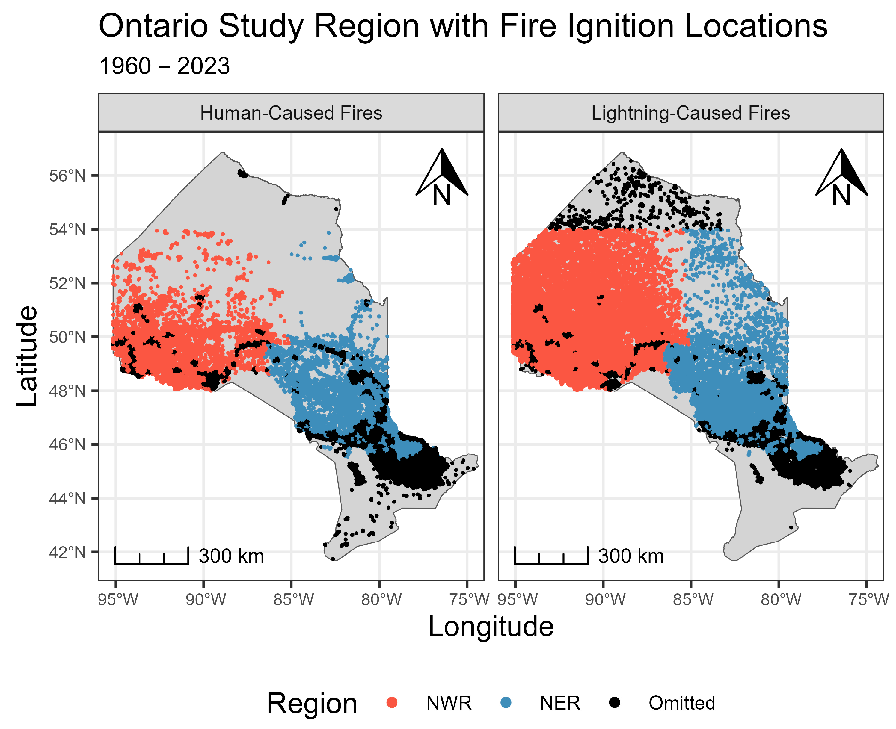
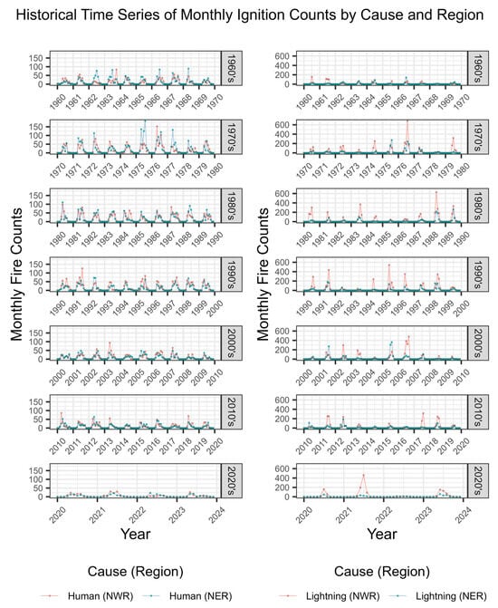
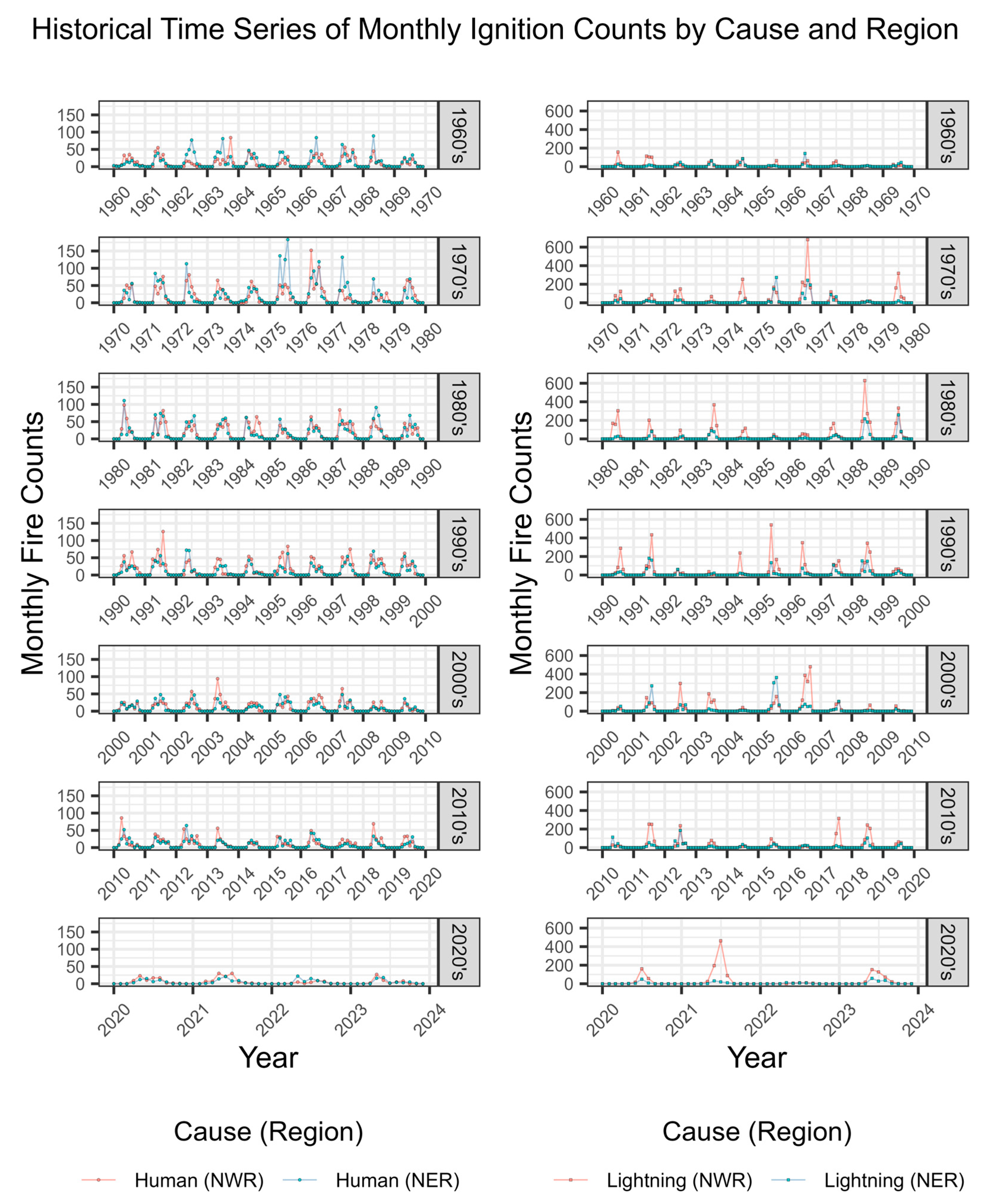
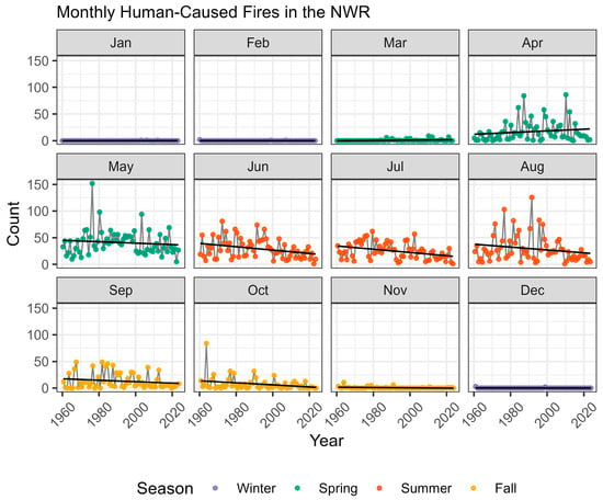
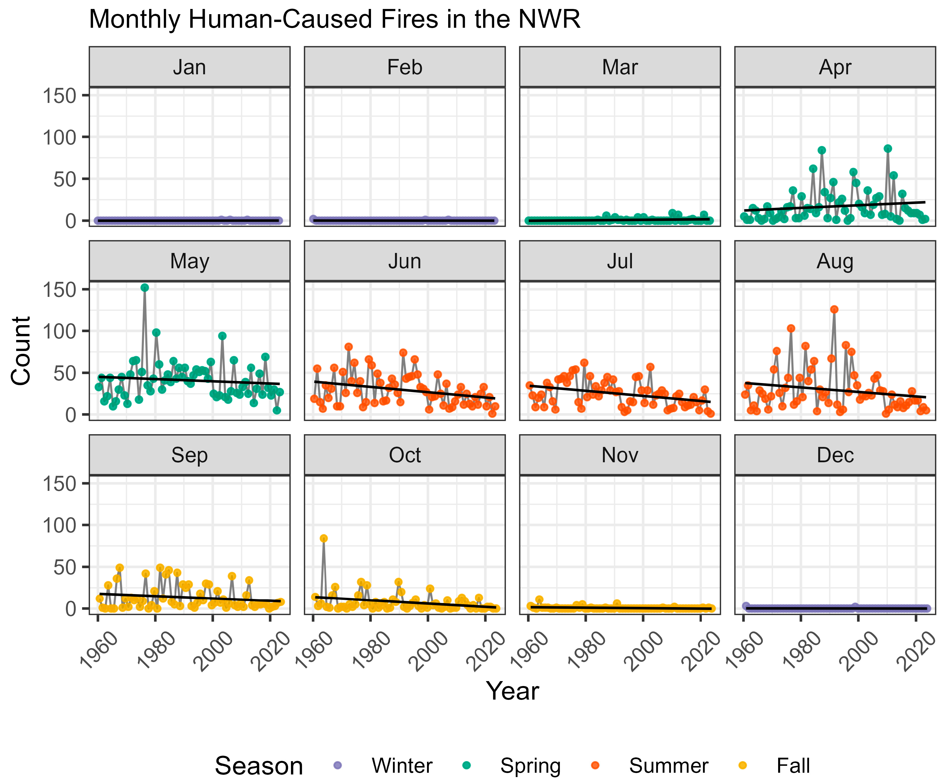
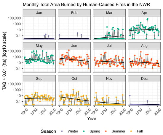
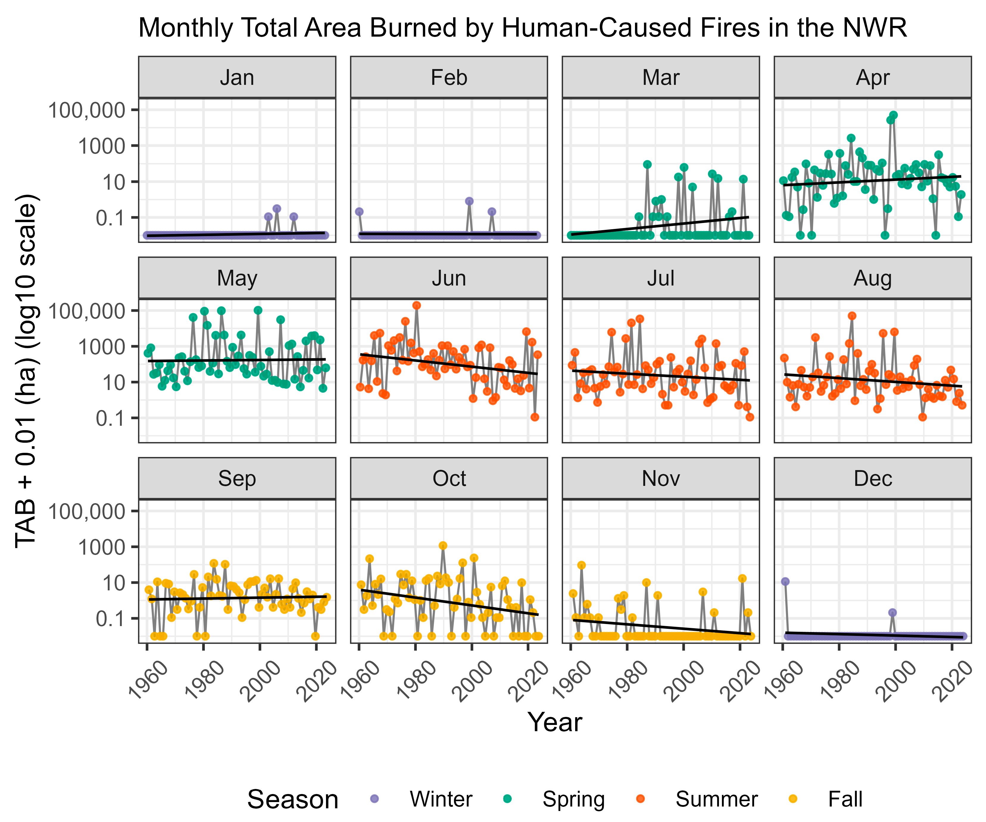
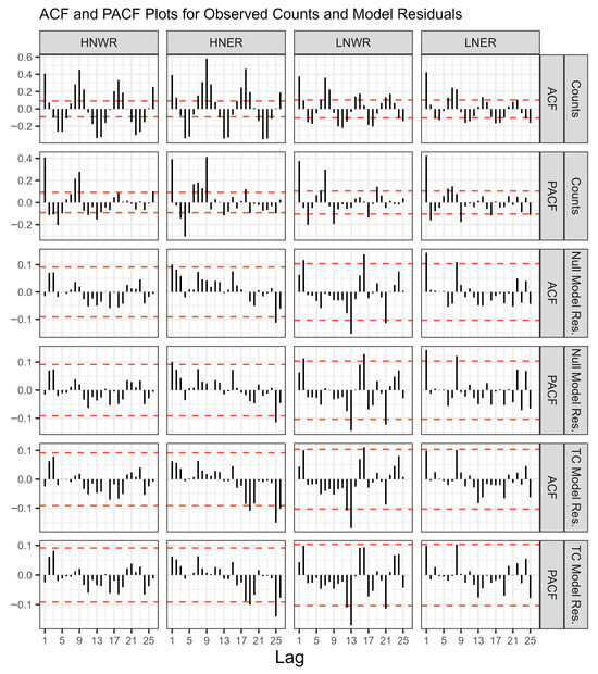
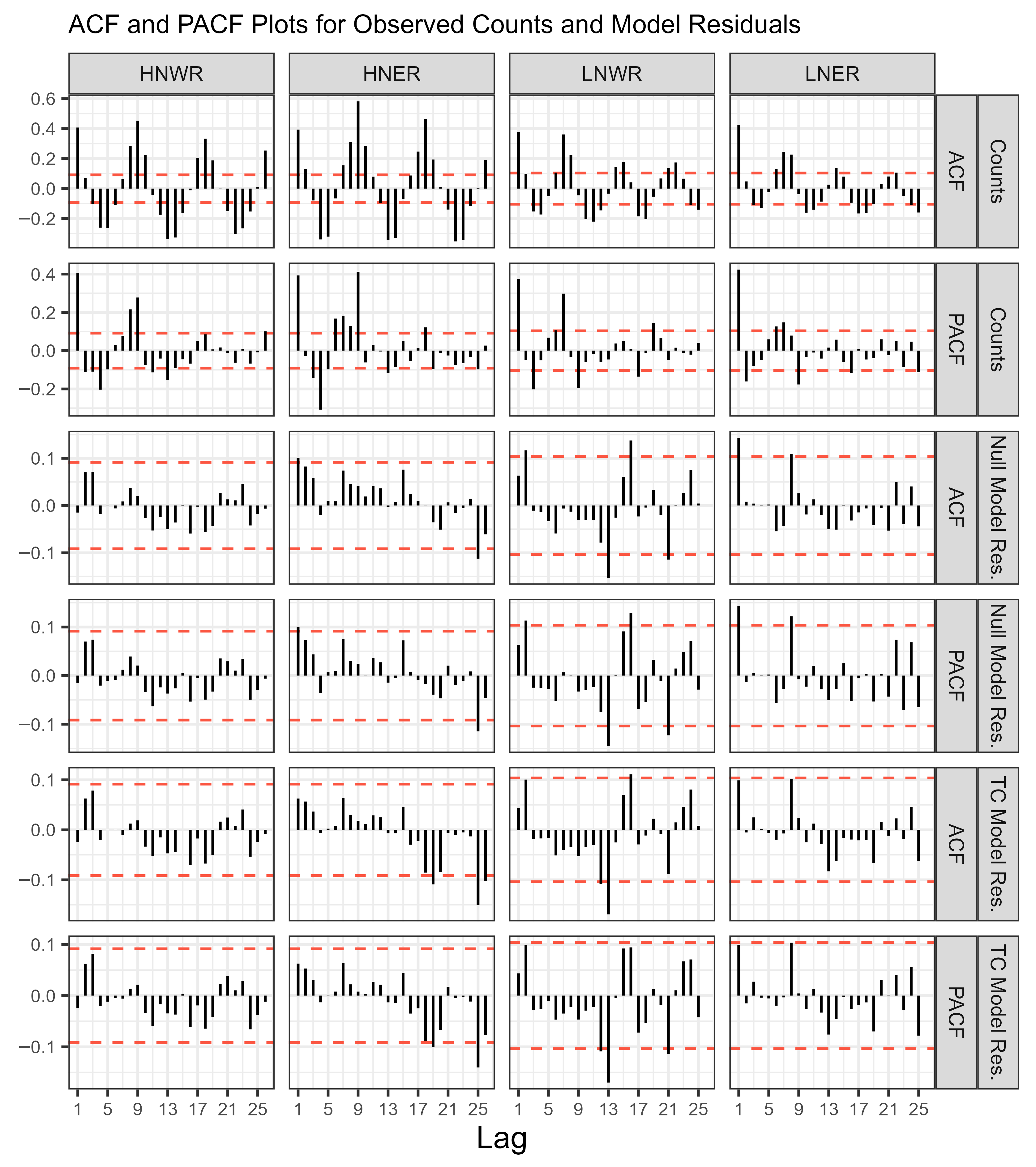
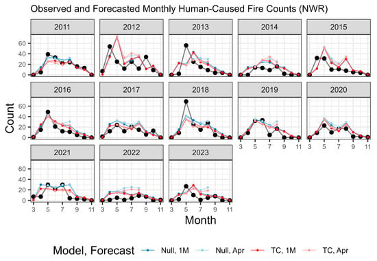
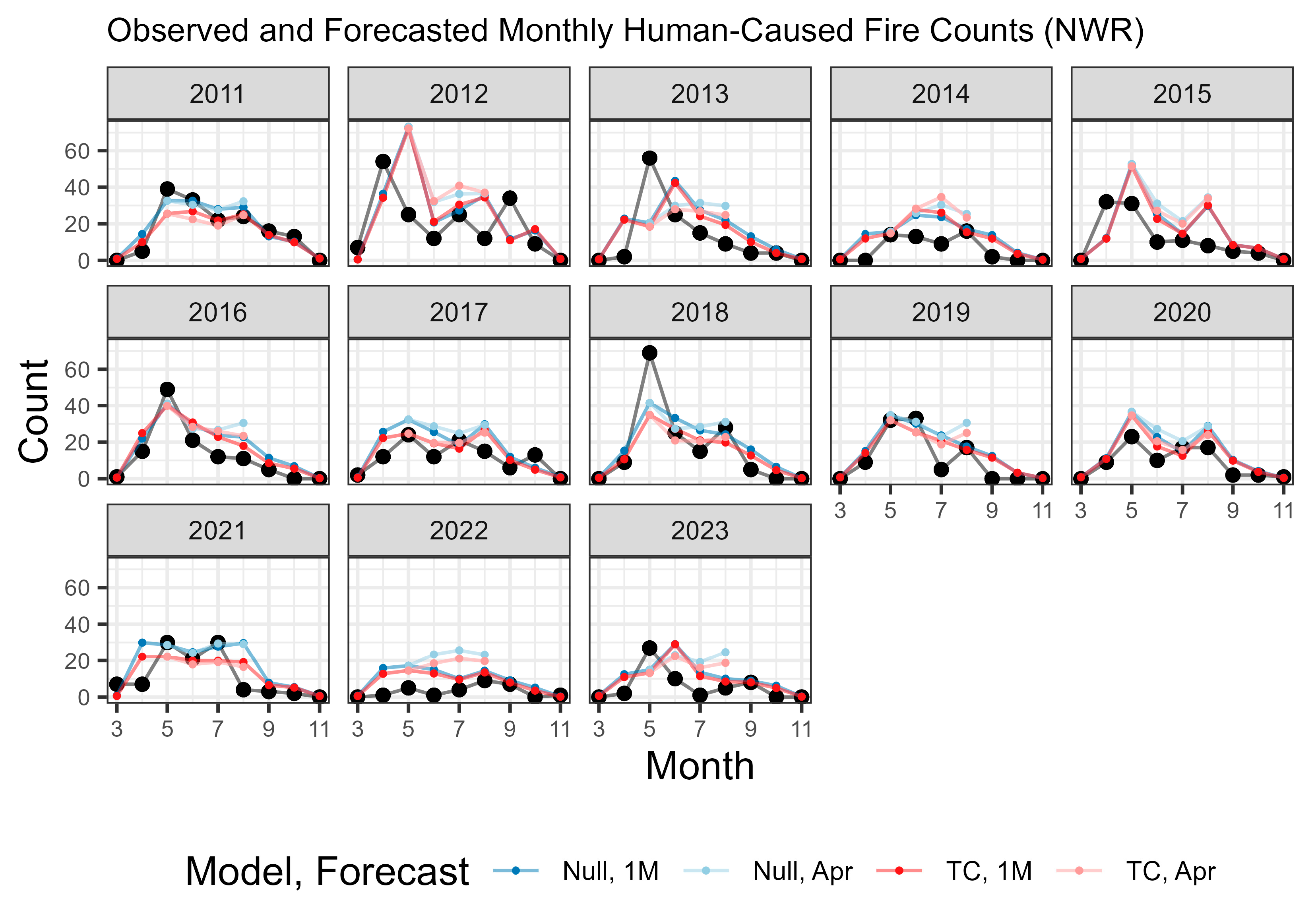

Disclaimer/Publisher’s Note: The statements, opinions and data contained in all publications are solely those of the individual author(s) and contributor(s) and not of MDPI and/or the editor(s). MDPI and/or the editor(s) disclaim responsibility for any injury to people or property resulting from any ideas, methods, instructions or products referred to in the content. |
© 2026 by the authors. Licensee MDPI, Basel, Switzerland. This article is an open access article distributed under the terms and conditions of the Creative Commons Attribution (CC BY) license.