Author Contributions
Conceptualization, X.L.; Data curation, X.L.; Formal analysis, T.H.; Investigation, L.S.; Methodology, M.Z.; Project administration, L.S.; Resources, J.L.; Software, S.Z.; Supervision, T.H.; Validation, S.S.; Visualization, S.S.; Writing—original draft, M.Z.; Writing—review and editing, X.L. All authors have read and agreed to the published version of the manuscript.
Figure 1.
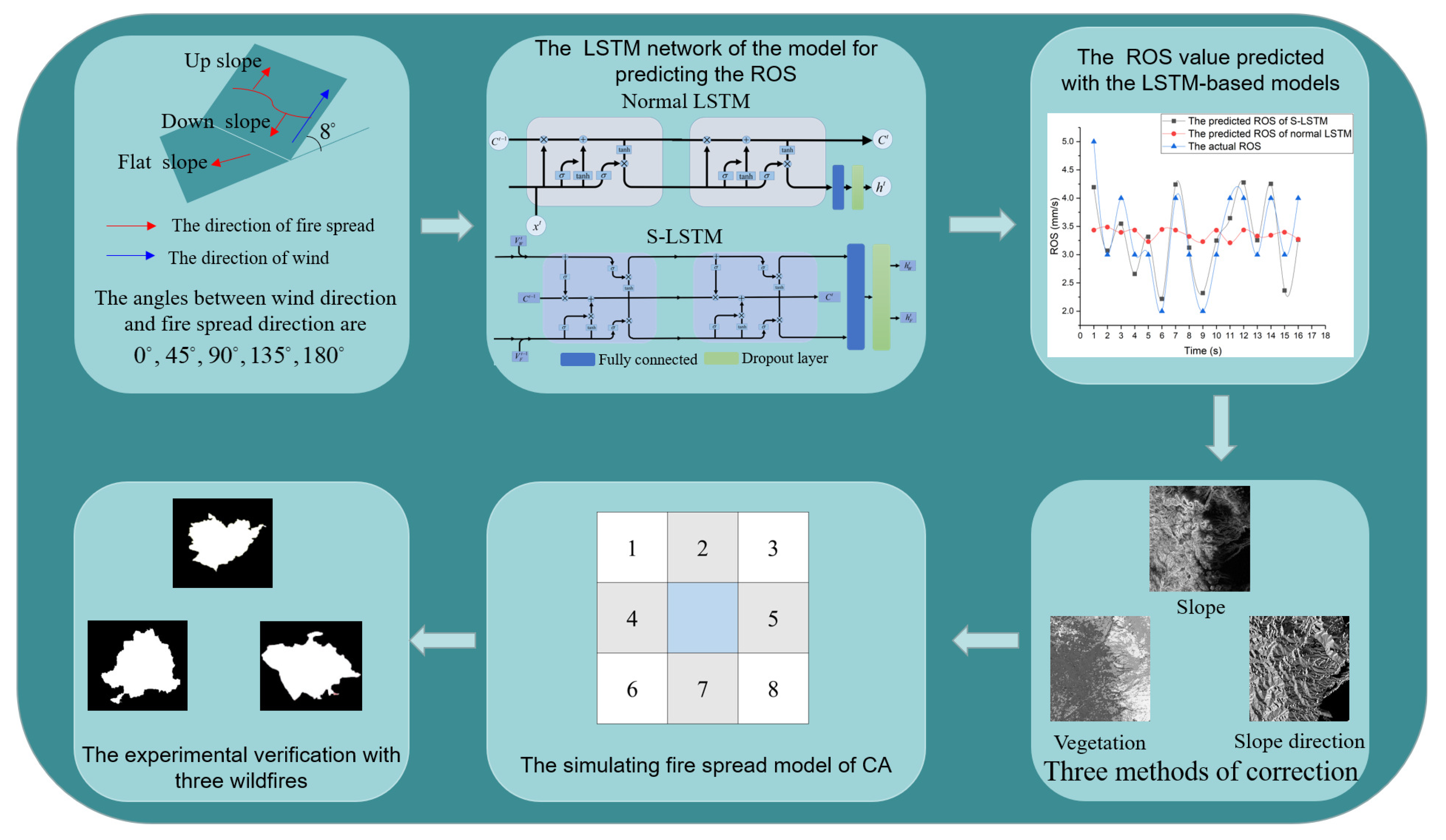
Flowchart for simulating forest fire spread based on CA with LSTM. Firstly, a fire spread rate model is designed and trained. Secondly, three kinds of fire rate correction methods are designed based on slope, slope direction, and vegetation, respectively. Finally, the model is verified with three wildfires, and the simulation result outperforms other models in the state of the art.
Figure 1.
Flowchart for simulating forest fire spread based on CA with LSTM. Firstly, a fire spread rate model is designed and trained. Secondly, three kinds of fire rate correction methods are designed based on slope, slope direction, and vegetation, respectively. Finally, the model is verified with three wildfires, and the simulation result outperforms other models in the state of the art.
Figure 2.
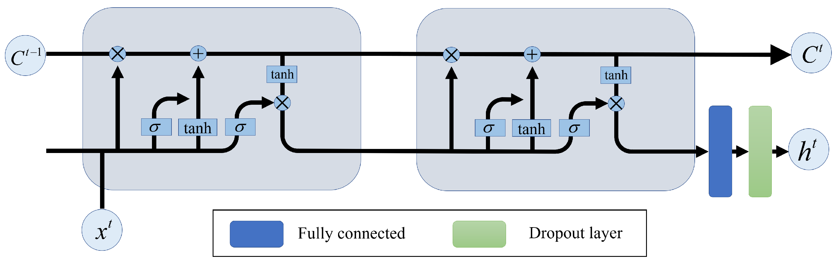
The LSTM cell structure. and are both one-dimensional matrices composed of wind speed and the ROS.
Figure 2.
The LSTM cell structure. and are both one-dimensional matrices composed of wind speed and the ROS.
Figure 3.
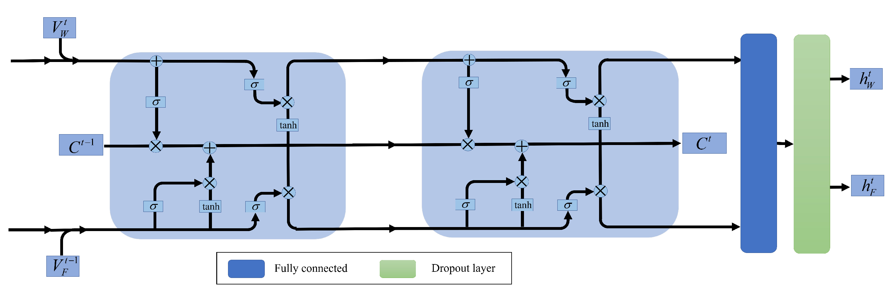
The S-LSTM cell structure. The ROS () and wind speed () as input to the S-LSTM model, respectively.
Figure 3.
The S-LSTM cell structure. The ROS () and wind speed () as input to the S-LSTM model, respectively.
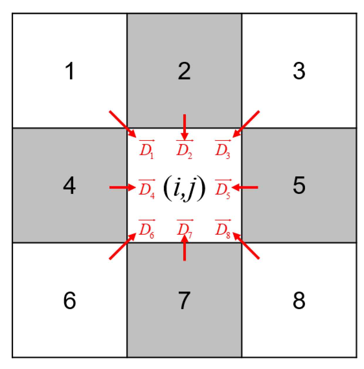
Figure 4.
Moore-neighbourhood type of two-dimensional CA. The cells of 2, 4, 5, and 7 are adjacent cells. The cells of 1, 3, 6, and 8 are sub-adjacent cells. denotes the direction from the i-th cell to the central cell.
Figure 4.
Moore-neighbourhood type of two-dimensional CA. The cells of 2, 4, 5, and 7 are adjacent cells. The cells of 1, 3, 6, and 8 are sub-adjacent cells. denotes the direction from the i-th cell to the central cell.
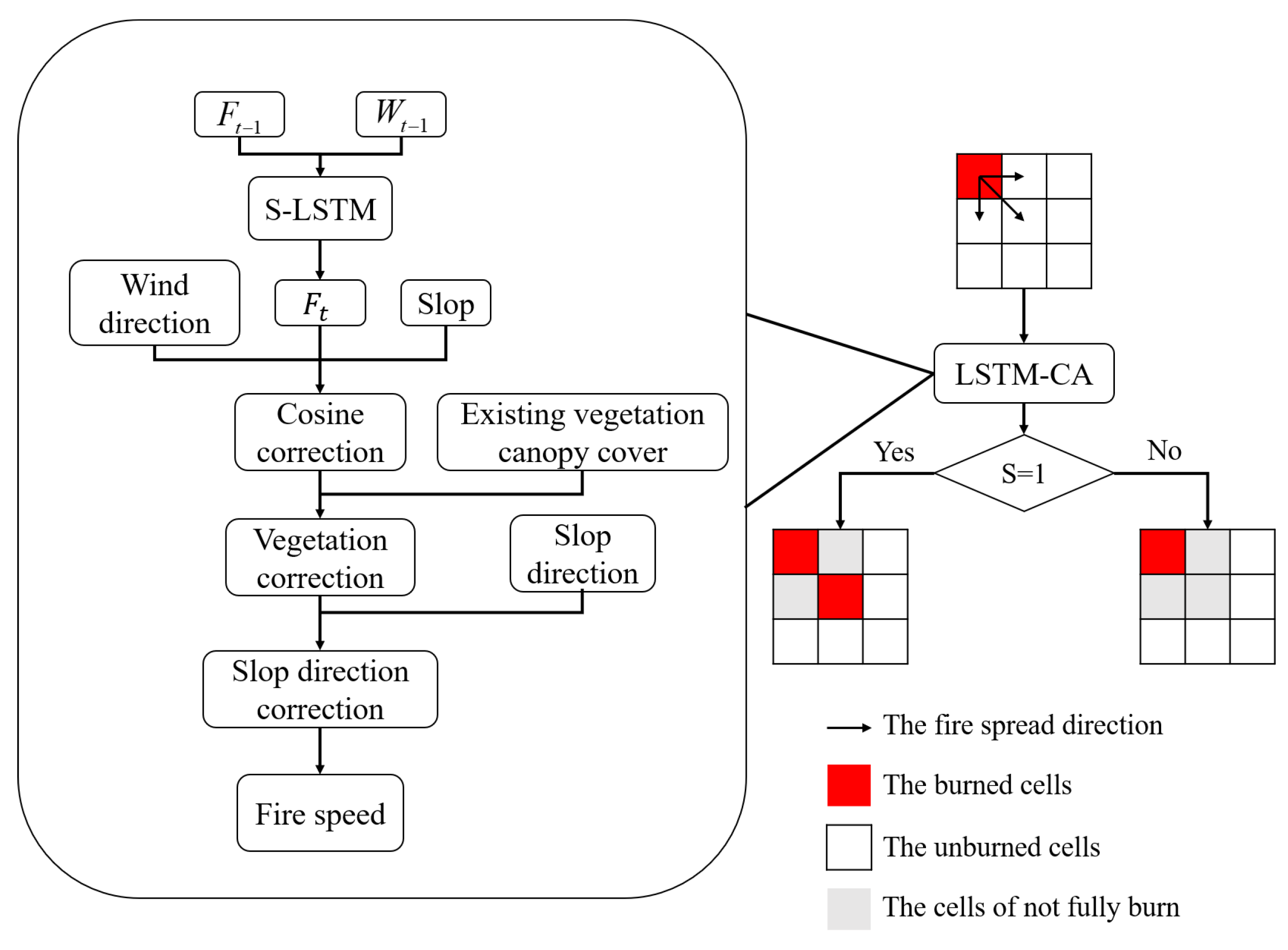
Figure 5.
The framework of the LSTM-CA model.
Figure 5.
The framework of the LSTM-CA model.
Figure 6.
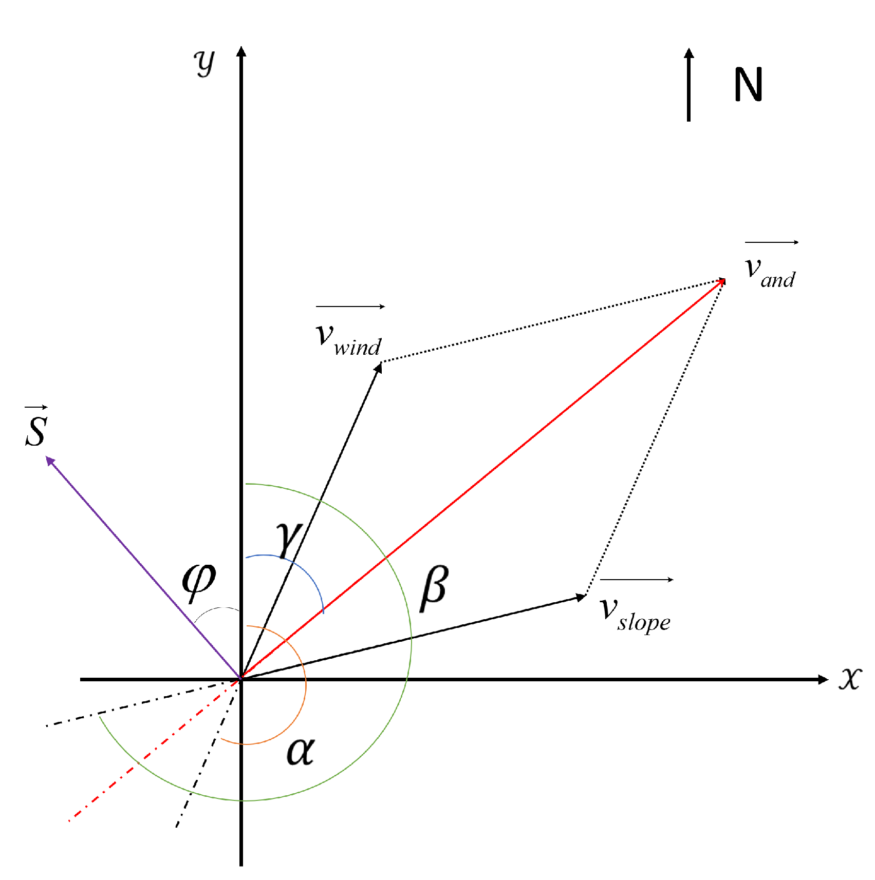
Wind direction and slope vector diagram. is the angle of wind direction, is the angle of slope direction, is the angle of main direction, and is the angle between the spread direction and the positive direction of the y-axis.
Figure 6.
Wind direction and slope vector diagram. is the angle of wind direction, is the angle of slope direction, is the angle of main direction, and is the angle between the spread direction and the positive direction of the y-axis.
Figure 7.
Example of fire spreading from the eight directional cells to the central cell. The adjacent cells spread to the central cell in a rectangle, and the sub-adjacent cells spread to the central cell in a quarter circle.
Figure 7.
Example of fire spreading from the eight directional cells to the central cell. The adjacent cells spread to the central cell in a rectangle, and the sub-adjacent cells spread to the central cell in a quarter circle.
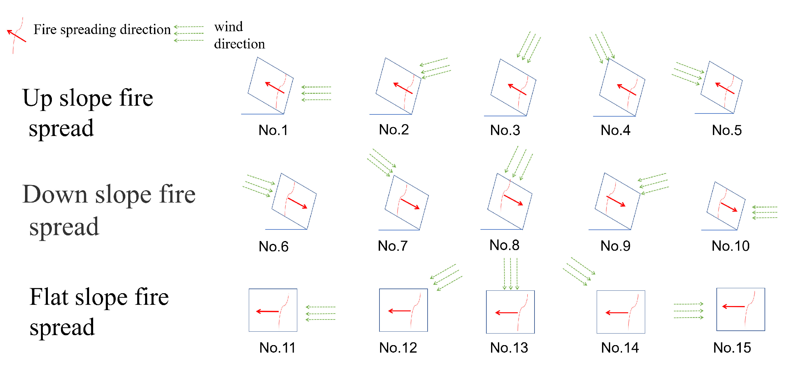
Figure 8.
Fifteen kinds of fire spread experiments. Three types of slope. Five kinds angle between fire spread direction and wind direction. From left to right, the angle between the wind direction and fire spread direction is 0, 45, 90, 135, and 180.
Figure 8.
Fifteen kinds of fire spread experiments. Three types of slope. Five kinds angle between fire spread direction and wind direction. From left to right, the angle between the wind direction and fire spread direction is 0, 45, 90, 135, and 180.
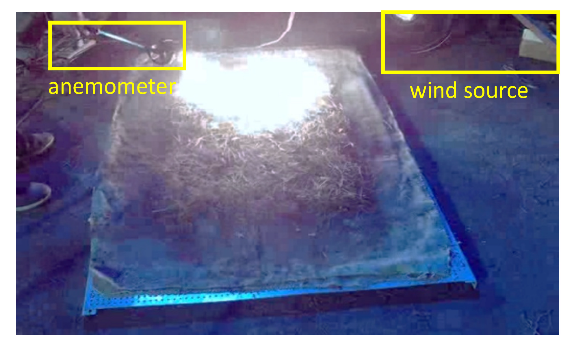
Figure 9.
Burning experiment configuration. The picture shows a hand-held anemometer in the upper-left corner and a wind source in the upper-right corner.
Figure 9.
Burning experiment configuration. The picture shows a hand-held anemometer in the upper-left corner and a wind source in the upper-right corner.
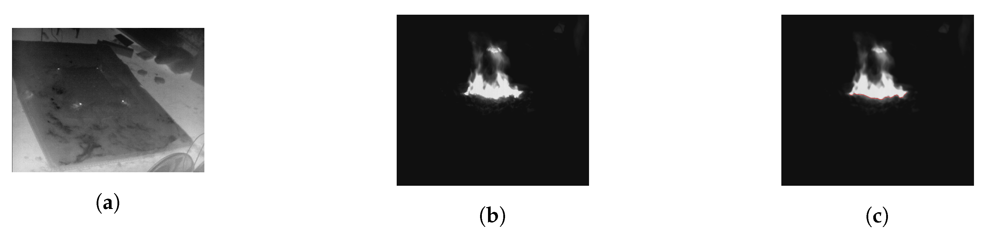
Figure 10.
The extraction process of the infrared image fire line. (a) is an infrared image with four calibration points, (b) is the image after perspective transformation, and (c) is the infrared image with the fire line.
Figure 10.
The extraction process of the infrared image fire line. (a) is an infrared image with four calibration points, (b) is the image after perspective transformation, and (c) is the infrared image with the fire line.
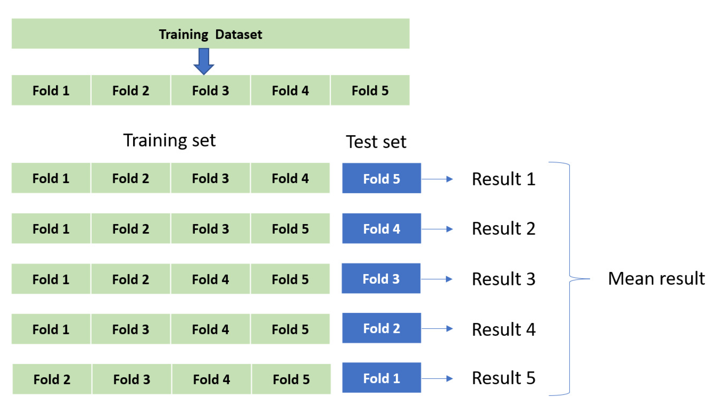
Figure 11.
Five-Fold cross Validation method. A total of 4/5 of the training data are used to train the model, 1/5 of the data are used for prediction, and the errors of the five prediction are averaged.
Figure 11.
Five-Fold cross Validation method. A total of 4/5 of the training data are used to train the model, 1/5 of the data are used for prediction, and the errors of the five prediction are averaged.
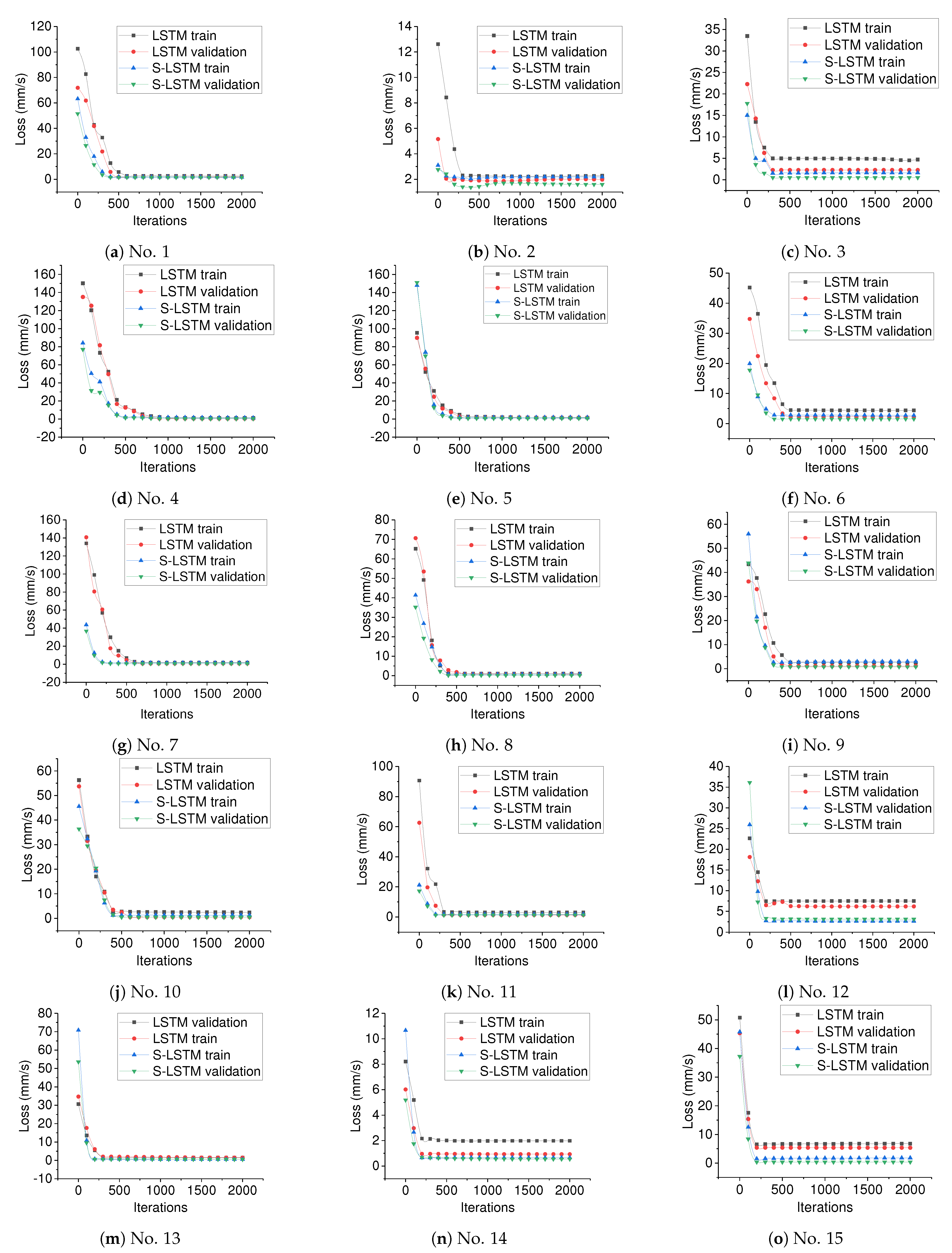
Figure 12.
The train loss and validation loss for both the normal LSTM and S-LSTM based on the dataset collected with the 15 kinds of configurations shown in
Table 2. The subfigures (
a–
o) are related to the data slots of No. (1–15) in
Table 2, respectively.
Figure 12.
The train loss and validation loss for both the normal LSTM and S-LSTM based on the dataset collected with the 15 kinds of configurations shown in
Table 2. The subfigures (
a–
o) are related to the data slots of No. (1–15) in
Table 2, respectively.
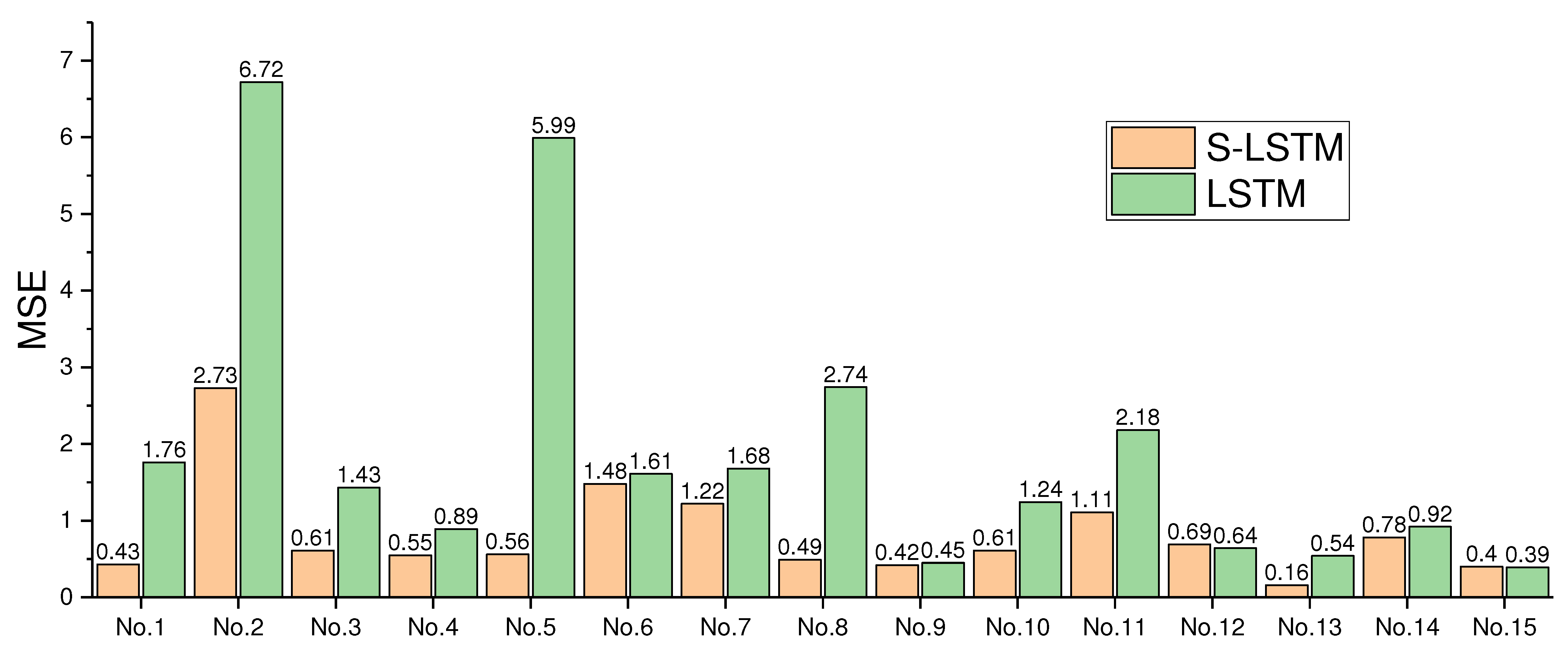
Figure 13.
The MSE of predicting the fire spread rate for both the normal LSTM and the S-LSTM based on the dataset collected with the 15 kinds of configurations shown in
Table 2. The histograms No. 1–15 are related to he data slots of No. (1–15) in
Table 2, respectively.
Figure 13.
The MSE of predicting the fire spread rate for both the normal LSTM and the S-LSTM based on the dataset collected with the 15 kinds of configurations shown in
Table 2. The histograms No. 1–15 are related to he data slots of No. (1–15) in
Table 2, respectively.
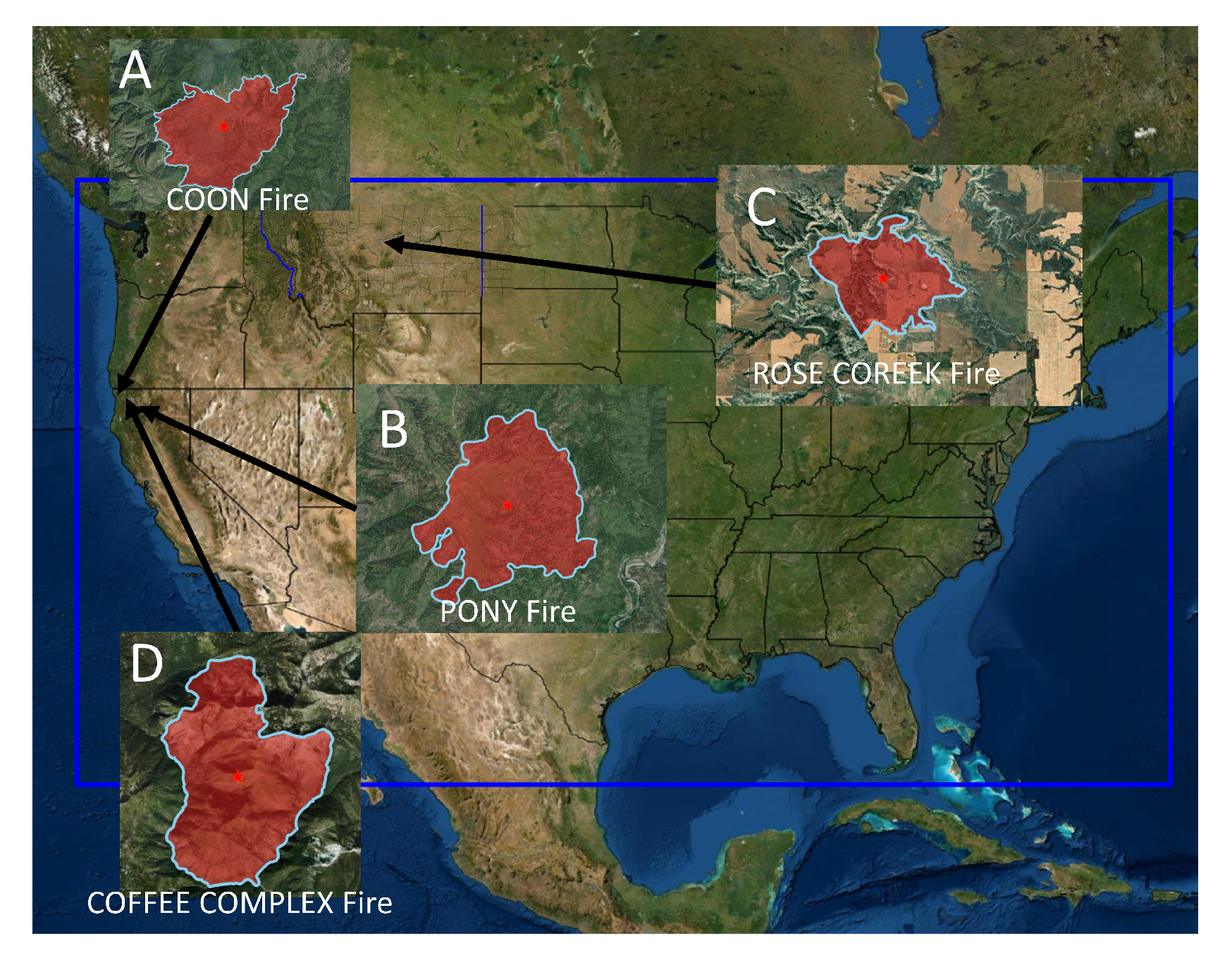
Figure 14.
The four wildfires that happend in the United States (the red stars show the starting point of each fire).
Figure 14.
The four wildfires that happend in the United States (the red stars show the starting point of each fire).
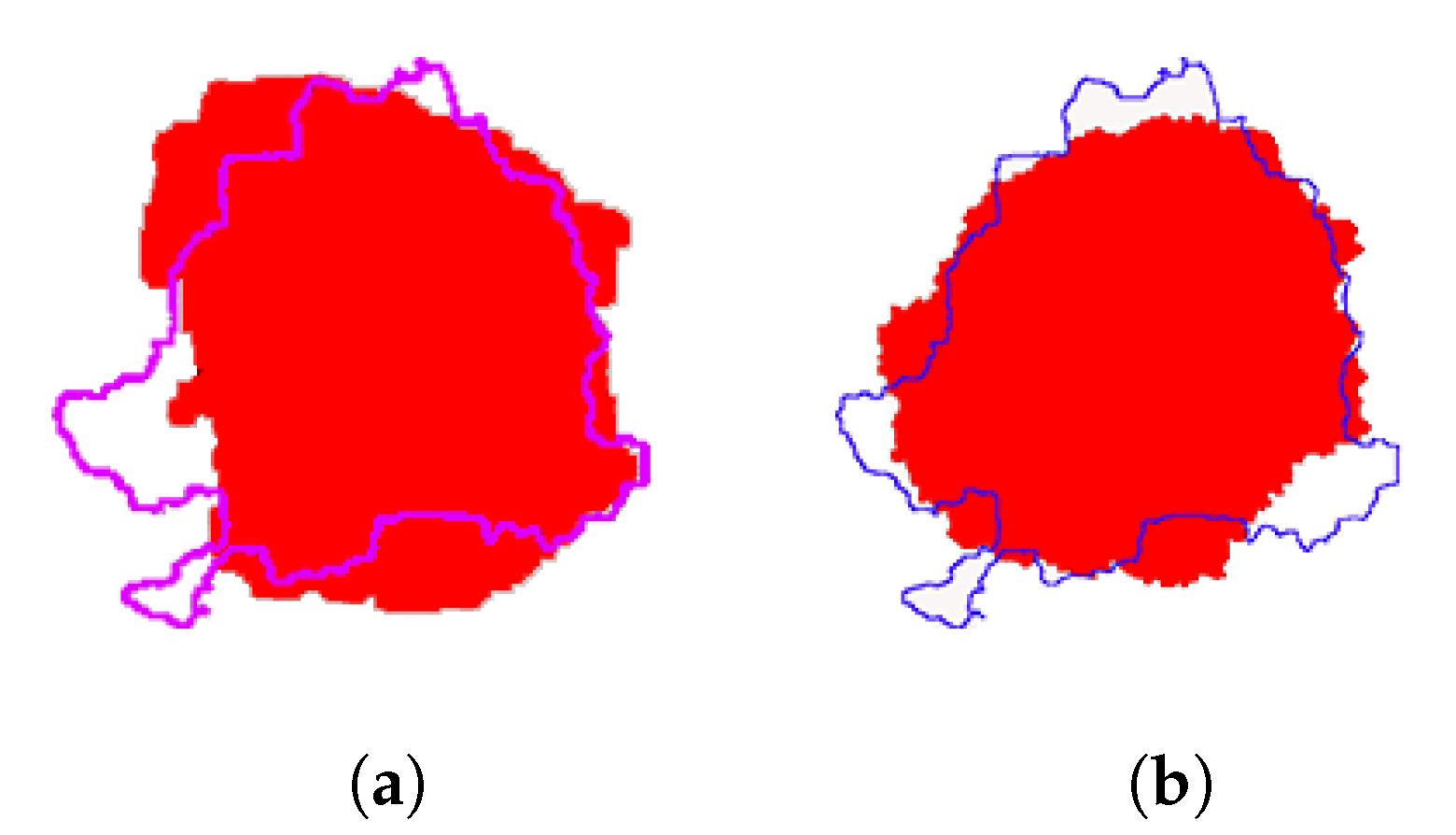
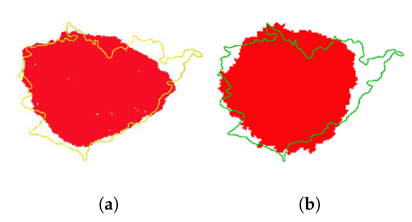
Figure 15.
The prediction and real burned region of COON wildfire. (a) The comparison of burned regions between LSTM-CA prediction and reality. (b) The comparison of burned regions between ELM-CA prediction and reality.
Figure 15.
The prediction and real burned region of COON wildfire. (a) The comparison of burned regions between LSTM-CA prediction and reality. (b) The comparison of burned regions between ELM-CA prediction and reality.
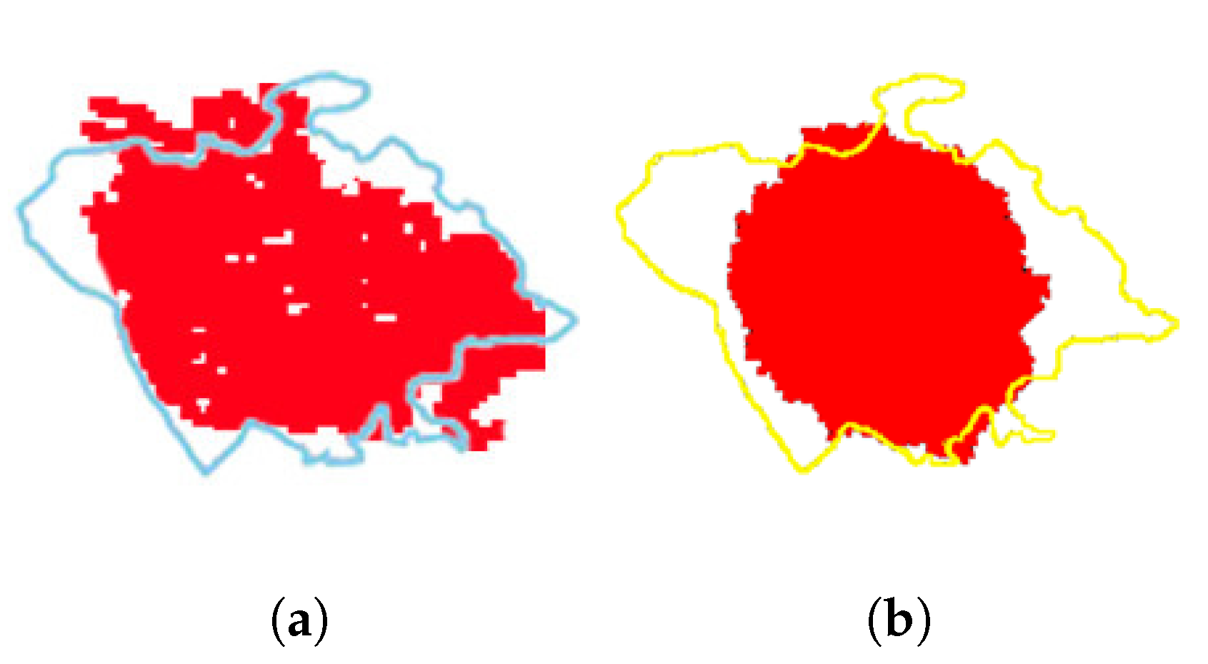
Figure 16.
The prediction and real burned region of PONY wildfire. (a) The comparison of burned regions between LSTM-CA prediction and reality. (b) The comparison of burned regions between ELM-CA prediction and reality.
Figure 16.
The prediction and real burned region of PONY wildfire. (a) The comparison of burned regions between LSTM-CA prediction and reality. (b) The comparison of burned regions between ELM-CA prediction and reality.
Figure 17.
The predicted and real burned regions of ROSE COREAK wildfire. (a) The comparison of burned regions between LSTM-CA prediction and reality. (b) The comparison of burned regions between ELM-CA prediction and reality.
Figure 17.
The predicted and real burned regions of ROSE COREAK wildfire. (a) The comparison of burned regions between LSTM-CA prediction and reality. (b) The comparison of burned regions between ELM-CA prediction and reality.
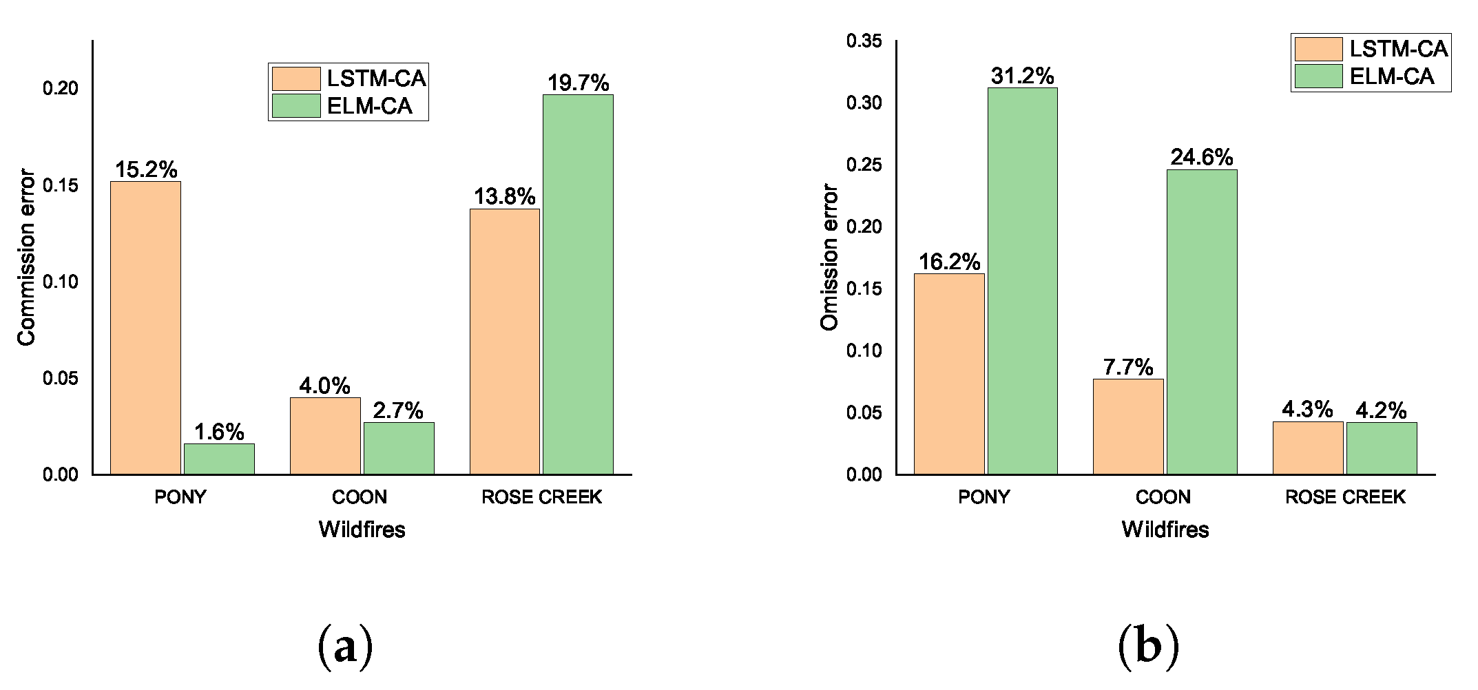
Figure 18.
The commission error and omission error for three wildfires simulated by models LSTM-CA and ELM-CA. (a) represents the commission error simulated by the two models. (b) represents the omission error simulated by the two models.
Figure 18.
The commission error and omission error for three wildfires simulated by models LSTM-CA and ELM-CA. (a) represents the commission error simulated by the two models. (b) represents the omission error simulated by the two models.
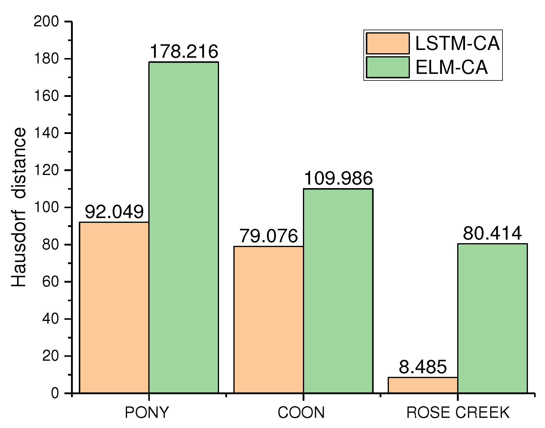
Figure 19.
Comparison of Hausdorff distance between simulated and actual results of the two models.
Figure 19.
Comparison of Hausdorff distance between simulated and actual results of the two models.
Table 1.
Unit vectors formed by adjacent cell and central cell.
Table 1.
Unit vectors formed by adjacent cell and central cell.
| The Spread of Vector | Mathematical Expression | Angle |
|---|
| [, ] | = 135° |
| [, ] | |
| [, ] | |
| [, ] | |
| [, ] | |
| [, ] | |
| [, ] | |
| [, ] | |
Table 2.
Fifteen kinds of fire spread test parameters. Three types of slope and five kinds angle between fire spread direction and wind direction.
Table 2.
Fifteen kinds of fire spread test parameters. Three types of slope and five kinds angle between fire spread direction and wind direction.
| NO. | Surface Area (m) | Slope | Angle between Wind Direction and Fire Spread Direction |
|---|
| 1 | 0.6 × 0.8 | Up slope/8° | 0° |
| 2 | 0.6 × 0.8 | Up slope/8° | 45° |
| 3 | 0.6 × 0.8 | Up slope/8° | 90° |
| 4 | 0.6 × 0.8 | Up slope/8° | 135° |
| 5 | 0.6 × 0.8 | Up slope/8° | 180° |
| 6 | 0.6 × 0.8 | Down slope/8° | 0° |
| 7 | 0.6 × 0.8 | Down slope/8° | 45° |
| 8 | 0.6 × 0.8 | Down slope/8° | 90° |
| 9 | 0.6 × 0.8 | Down slope/8° | 135° |
| 10 | 0.6 × 0.8 | Down slope/8° | 180° |
| 11 | 0.6 × 0.8 | Flat slope/0° | 0° |
| 12 | 0.6 × 0.8 | Flat slope/0° | 45° |
| 13 | 0.6 × 0.8 | Flat slope/0° | 90° |
| 14 | 0.6 × 0.8 | Flat slope/0° | 135° |
| 15 | 0.6 × 0.8 | Flat slope/0° | 180° |
Table 3.
The hyperparameters for training the LSTM-based model (S-LSTM).
Table 3.
The hyperparameters for training the LSTM-based model (S-LSTM).
| LSTM Layers | Learning Rate | Units | Batch Size | Time Step | Iterations |
|---|
| 2 | 0.001 | 10 | 15 | 5 | 1200 |
Table 4.
The confusion matrix values of simulation results of the LSTM-CA model for three wildfires.
Table 4.
The confusion matrix values of simulation results of the LSTM-CA model for three wildfires.
| | True Positive (TP) | False Positive (FP) | False Negative (FN) | True Negative (TN) |
|---|
| PONY | 28.5% | 5.1%f | 5.5% | 60.9% |
| COON | 24.0% | 1.0% | 2.0% | 73.0% |
| ROSE CREEK | 31.2% | 5.0% | 1.4% | 62.4% |
Table 5.
The confusion matrix values of simulation results of the ELM-CA model for three wildfires.
Table 5.
The confusion matrix values of simulation results of the ELM-CA model for three wildfires.
| | True Positive (TP) | False Positive (FP) | False Negative (FN) | True Negative (TN) |
|---|
| PONY | 37.7% | 0.6% | 17.1% | 44.6% |
| COON | 25.2% | 0.7% | 8.2% | 65.9% |
| ROSE CREEK | 29.3% | 7.2% | 1.3% | 62.2% |
Table 6.
The KAPPA coefficient of the LSTM-CA model’s simulation results of three wildfires.
Table 6.
The KAPPA coefficient of the LSTM-CA model’s simulation results of three wildfires.
| | PONY | COON | ROSE CREEK |
|---|
| 0.89 | 0.97 | 0.94 |
| 0.55 | 0.62 | 0.55 |
| K | 0.76 | 0.92 | 0.86 |
Table 7.
The KAPPA coefficient of the ELM-CA model’s simulation results of three wildfires.
Table 7.
The KAPPA coefficient of the ELM-CA model’s simulation results of three wildfires.
| | PONY | COON | ROSE CREEK |
|---|
| 0.82 | 0.91 | 0.92 |
| 0.49 | 0.58 | 0.55 |
| K | 0.65 | 0.79 | 0.81 |


 ,
, 


