A Theoretical Study of the Ionization States and Electrical Conductivity of Tantalum Plasma

Abstract

Tantalum is extensively used in inertial confinement fusion research for targets in radiation transport experiments, hohlraums in magnetized fusion experiments, and lining foams for hohlraums to suppress wall motions. To comprehend the physical processes associated with these applications, detailed information regarding the ionization composition and electrical conductivity of tantalum plasma across a wide range of densities and temperatures is essential. In this study, we calculate the densities of ionization species and the electrical conductivity of partially ionized, nonideal tantalum plasma based on a simplified theoretical model that accounts for high ionization states up to the atomic number of the element and the lowering of ionization energies. A comparison of the ionization compositions between tantalum and copper plasmas highlights the significant role of ionization energies in determining species populations. Additionally, the average electron–neutral momentum transfer cross-section significantly influences the electrical conductivity calculations, and calibration with experimental measurements offers a method for estimating this atomic parameter. The impact of electrical conductivity in the intermediate-density range on the laser absorption coefficient is discussed using the Drude model.

1. Introduction

Tantalum (Ta) plays a crucial role in various applications, particularly in inertial confinement fusion (ICF). For instance, in magnetized ICF experiments, high electrical resistivity of the hohlraum is required to facilitate rapid magnetic field diffusion. It has been shown that a gold–tantalum alloy with approximately 80% Ta exhibits a maximum electrical resistivity of over 300 $\mathsf{\mu }\mathsf{\Omega }$·cm, roughly 150 times larger than that of pure gold [1], making Ta an attractive doping material for hohlraums. Additionally, tantalum oxide aerogels serve as significant target materials for radiation transport experiments due to their high-Z elements and low densities [2], where the ionization composition of Ta plasma affects both the yield and transport properties of X-ray. Tantalum oxide foams have also been utilized as lining materials for ICF hohlraums in indirect-driven experiments to mitigate wall motions [3,4] or to suppress stimulated Brillouin scattering [5].

To understand the physical processes related to the various applications of tantalum in ICF, a thorough investigation of the ionization states and electrical conductivity of tantalum plasma is essential. The ionization composition of Ta plasmas reveals the proportions of different charge states, which influence atomic processes such as electron–ion and electron–neutral collisions, excitation, ionization, and radiation. Furthermore, it significantly affects the electrical conductivity of Ta plasma, which in turn impacts physical processes like magnetic field diffusion and laser energy deposition.

Despite the critical importance of tantalum plasma in ICF applications, systematic investigations into its thermophysical and electrical properties remain notably scarce. Zhernokletov et al. [6] measured the pressure and density of tantalum along release isentropes at densities exceeding the critical density. Miljacic et al. [7] utilized first-principles methods to investigate the equation of state of Ta for solid, liquid, and gaseous phases. DeSilva and Vunni [8] measured the electrical conductivity of Ta plasma through wire explosion experiments within a density range of approximately 0.1 g/cm³ to several g/cm³. Apfelbaum [9] conducted a theoretical study on the pressure, internal energy, and electrical conductivity of Ta plasma, employing generalized chemical models and the relaxation time approximation. However, the model imposed an artificial constraint limiting ion charge states to Z≤ +3, potentially introducing non-negligible errors. While their work reported the average ionization state of Ta plasma at 13,000 K and the electrical conductivity at specific internal energy levels, the critical aspect of detailed ionization state distributions, particularly the population fractions of different charge states, was not rigorously addressed.

In this study, we conducted detailed calculations of the charge species in tantalum plasmas, including higher ionization states. By employing a more accurate representation of the Coulomb logarithm in the nonideal regime, we also calculated the electrical conductivity of Ta plasmas. We discussed the effects of the average electron–neutral momentum transfer cross section on electrical conductivity in the intermediate-density region. Considering foam-related application scenarios, we examined the influence of electrical conductivity on the laser absorption coefficient using the Drude model.

2. Methods

2.1. Ionized Species

In a plasma, the degree of ionization is a crucial parameter that depends on temperature and the balance between ionization and recombination processes. Harris et al. [10] introduced the free-energy minimization method (FEMM) to determine the distribution of species that minimizes the total Gibbs free energy of the system. This method is particularly effective in multi-temperature plasmas, where different species may possess varying temperatures. By minimizing the free energy, one can ascertain the equilibrium composition of the plasma, including the concentrations of various ionization states of the atoms and molecules present.

In practice, the FEMM can yield a system of minimization equations akin to the Saha equations (hereafter referred to as the nonideal Saha equations). However, it is essential to account for the lowering of ionization energies, specifically

$${\displaystyle \frac{n_{i+1}{n}_e}{n_i}}=2{\displaystyle \frac{Q_{i+1}}{Q_i}}{\left({\displaystyle \frac{2\pi m_e{k}_{B}T}{h^2}}\right)}^{3/2}·exp\left(-{\displaystyle \frac{I_i-\Delta I_i}{k_{B}T}}\right),$$

(1)

where $(n_i,n_e)$ are the number densities of the ith ionized species and electrons, and $(Q_i,I_i,\Delta I_i)$ are the partition function, ionization energy, and lowering of the ionization energy of the ith ionization level, respectively. Physical constants $(m_e,k_B,h)$ represent the electron mass and Boltzmann and Planck constants, respectively.

In principle, the total internal partition function $Q_i$ can be calculated as follows [11]:

$$Q_i=\sum _{n=1}^{\infty }{g}_{i,n}exp\left(-{\displaystyle \frac{E_{i,n}}{k_{B}T}}\right),$$

(2)

where $E_{i,n}$ is the nth excitation energy of species i and $g_{i,n}$ is the corresponding statistical weight. In practice, the summation is necessarily limited to a maximum level of $n=n^{*}$ with a termination energy of $E_{n^{*}}$. The selection of the termination energy $E_{n^{*}}$ is arbitrary. For instance, in Ref. [11], it is assumed that $E_{n^{*}}\le I_i-\Delta I_i$, resulting in the partition function being a function of both temperature T and density $\rho$. However, in this study, the effects of electronic excited states are neglected, and the partition functions are approximated by the statistical weights of the ground states, i.e., $Q_i\approx g_{i,0}$.

The lowering of ionization energies $\Delta I_i$ is determined through a revised approach introduced in Ref. [12] and is expressed as follows:

$$\Delta I_i={\displaystyle \frac{(i+1)e^2}{4\pi {\epsilon }_0{R}_i}},$$

(3)

where e is the electron charge, ${\epsilon }_0$ is the permittivity of vacuum, and $R_i$ is some characteristic radius. The characteristic radius $R_i$ varies according to different models. For example, in the Debye model [13] for low-density and weakly nonideal plasmas $R_i={\lambda }_D$, where ${\lambda }_D$ is the Debye length. On the other hand, in the ion-sphere model [14] for high-density and strong nonideal plasmas $R_i=2a_i/3$, where $a_i$ is the ion-sphere radius.

For moderate-density and nonideal plasmas, several models have been proposed to interpolate between the Debye model and the ion-sphere model. One of the most prevalent approaches [12] is to connect these two models by defining $R_i$ as follows:

$$R_i=\sqrt{{\lambda }_D^2+{\left({\displaystyle \frac{2}{3}}{a}_i\right)}^2}.$$

(4)

Furthermore, various methods for calculating $a_i$ have been introduced. For instance, Ecker and Kröll [15] assumed that all ions possess identical ion-sphere radii and defined $a_i$ as follows:

$$a_i={\left({\displaystyle \frac{3}{4\pi n_H(1+{\alpha }_e)}}\right)}^{1/3},$$

(5)

where $n_H={\sum }_i{n}_i$ is the number density of heavy particles and ${\alpha }_e$ is the average ionization state of the plasma. Alternatively, Stewart and Pyatt Jr. [16] considered the free electrons within the cell and adopted the following formula:

$$a_i={\left({\displaystyle \frac{3i}{4\pi n_e}}\right)}^{1/3}.$$

(6)

However, this method assigns a volume of zero to neutrals and does not result in a decrease in their ionization energies. Zaghloul [12] posited that the ion-cell volume is proportional to the number of inhabitants within the cell and derived the following expression:

$$a_i={\left({\displaystyle \frac{3(i+1)}{4\pi n_H(1+{\alpha }_e)}}\right)}^{1/3}.$$

(7)

Inthis method, ions with different charge states acquire varying radii, and the cell volumes for neutral species are also properly accounted for.

2.2. Nonideal Saha Equations

The system of nonideal Saha equations is solved in conjunction with the following conservation laws of mass and charge:

$$\begin{array}{ccc}\hfill \rho & =& \sum _i{m}_{\mathrm{atom}}{n}_i,\hfill \end{array}$$

(8)

$$\begin{array}{ccc}\hfill {\alpha }_e& =& {\displaystyle \frac{n_e}{{\sum }_i{n}_i}},\hfill \end{array}$$

(9)

where $\rho$ is the average mass density of the plasma and $m_{\mathrm{atom}}$ is the atomic mass of ions. The contribution of electrons to atomic mass is often neglected, and ions with different charge states are assumed to have the same atomic mass. Atomic parameters are from the databases provided by the National Institute of Standards and Technology (NIST) [17].

The numerical algorithm used to solve the nonideal Saha equations is similar to the one proposed by Trayner and Glowacki [18]. The set of Equation (1) is first rewritten in the following form:

$${\displaystyle \frac{n_{i+1}}{n_i}}={\displaystyle \frac{1+{\alpha }_e}{{\alpha }_e}}{\displaystyle \frac{2Q_{i+1}}{Q_i}}{\left({\displaystyle \frac{2\pi m_e{k}_{B}T}{h^2}}\right)}^{3/2}·exp\left(-{\displaystyle \frac{I_i-\Delta I_i}{k_{B}T}}\right).$$

(10)

Definingthe right-hand side of the above equation as $L_{i+1}$ yields the following recurrence relation for ${\alpha }_i$ (with the exception of ${\alpha }_0$):

$${\alpha }_i={\alpha }_{i-1}{L}_i,$$

(11)

where ${\alpha }_i\equiv n_i/n_H$. This gives

$${\alpha }_i=\left(\prod _{j=1}^i{L}_j\right){\alpha }_0,$$

(12)

and ${\alpha }_0$ can be determined by

$${\alpha }_0=1-\left[\sum _{i=1}^n\left(\prod _{j=1}^i{L}_j\right)\right]{\alpha }_0\Rightarrow {\alpha }_0={\displaystyle \frac{1}{1+\left[{\sum }_{i=1}^n\left({\prod }_{j=1}^i{L}_j\right)\right]}}.$$

(13)

Inthis procedure, for a given value of ${\alpha }_e$, we first calculate $L_i$s in order to obtain ${\alpha }_0$ from Equation (13). Notice that excluding electronic excitation states means $Q_i\approx g_{i,0}$, while including excitation states means that additional calculations of $Q_i$s according to Equation (2) are required. With ${\alpha }_0$ obtained, ${\alpha }_i$ can be readily calculated from Equation (12), which in turn yields a new value of ${\alpha }_e^{\prime }$ that is generally different from ${\alpha }_e$. By solving the equation of ${\alpha }_e-{\alpha }_e^{\prime }=0$, we obtain the converged value of ${\alpha }_e$ along with the converged set of ${\alpha }_i$. For 10,000 ≤ T ≤ 50,000 K and 10⁻⁵ ≤$\rho$ ≤ 10¹ g/cm⁻³, the function $\Delta {\alpha }_e\equiv {\alpha }_e-{\alpha }_e^{\prime }$ is monotonically increasing, with $\Delta {\alpha }_e<0$ at ${\alpha }_e={10}^{-12}$ and $\Delta {\alpha }_e>0$ at ${\alpha }_e=Z_{\mathrm{atom}}$ ($Z_{\mathrm{atom}}$ is the atomic number). Therefore, a bisection algorithm is applied to obtain a linear and safe convergence of ${\alpha }_e$.

2.3. Electrical Conductivity

A linear mixture rule for additive effective collision frequencies, which yields exact values at the limiting boundaries, can be formulated as described in Ref. [19]:

$${\displaystyle \frac{1}{\sigma }}={\displaystyle \frac{1}{{\sigma }_{ei}}}+{\displaystyle \frac{1}{{\sigma }_{en}}},$$

(14)

where ${\sigma }_{ei}$ and ${\sigma }_{en}$ are the electrical conductivities associated with the electron–ion and electron–neutral collisions, respectively. The electron–neutral conductivity is simply expressed as follows [12]:

$${\sigma }_{en}=\sqrt{{\displaystyle \frac{\pi }{8m_e{k}_{B}T}}}{\displaystyle \frac{{\alpha }_e{e}^2}{{\alpha }_0{\overline{Q}}_{en}}},$$

(15)

where ${\overline{Q}}_{en}$ is the average electron–neutral momentum transfer cross-section [20,21]. In the following calculations, ${\overline{Q}}_{en}$≈ 1.5 × 10⁻¹⁸ m² for copper is adopted [12] (see Section 3.1), while for tantalum ${\overline{Q}}_{en}$ is set to 1.5 × 10⁻¹⁸, 1.5 × 10⁻¹⁹, and 1.5 × 10⁻²⁰ m² in order to discuss its effects on electrical conductivity calculations (see Section 3.4).

The electron–ion conductivity can be expressed using the Spitzer-Härm formula [22] for fully ionized plasma, taking into account electron–electron collisions:

$${\sigma }_{ei}={\displaystyle \frac{T^{3/2}}{38{\alpha }_e}}{\displaystyle \frac{{\gamma }_e\left({\alpha }_e\right)}{ln\mathsf{\Lambda }}},$$

(16)

where $ln\mathsf{\Lambda }$ is the Coulomb logarithm representing the classical collision cross-section integral for electrons’ interaction with ions of charge ${\alpha }_e$ and can be expressed as follows:

$$\mathsf{\Lambda }\approx \left(2.4287{\mathsf{\Lambda }}_B\right){\left[1+{\left({\displaystyle \frac{{\overline{a}}_i}{2.4287{\mathsf{\Lambda }}_B{\overline{b}}_0}}\right)}^4\right]}^{1/4},$$

(17)

where $({\overline{a}}_i,{\overline{b}}_0)$ represent the average ion-sphere radius and impact parameter [23]. The quantum mechanical parameter ${\mathsf{\Lambda }}_B\equiv {\lambda }_D/{\lambda }_0$, where ${\lambda }_D$ is the Debye length and ${\lambda }_0=\hslash /\sqrt{2M_r{k}_{B}T}$ is the average electron thermal wavelength ($M_r$ is the reduced mass of the interacting particles). This expression reduces to the Born approximation with the Debye potential case at low density and to the ion-sphere case at high density, and has been applied for various elements such as Cu [12], W [20], etc.

The factor ${\gamma }_e\left({\alpha }_e\right)$ accounts for the electron–electron scattering and reads as follows [12]:

$${\gamma }_e\left(x\right)={\displaystyle \frac{3\pi }{32}}\left(1+{\displaystyle \frac{153x^2+509x}{64x^2+345x+288}}\right).$$

(18)

3. Results and Discussion

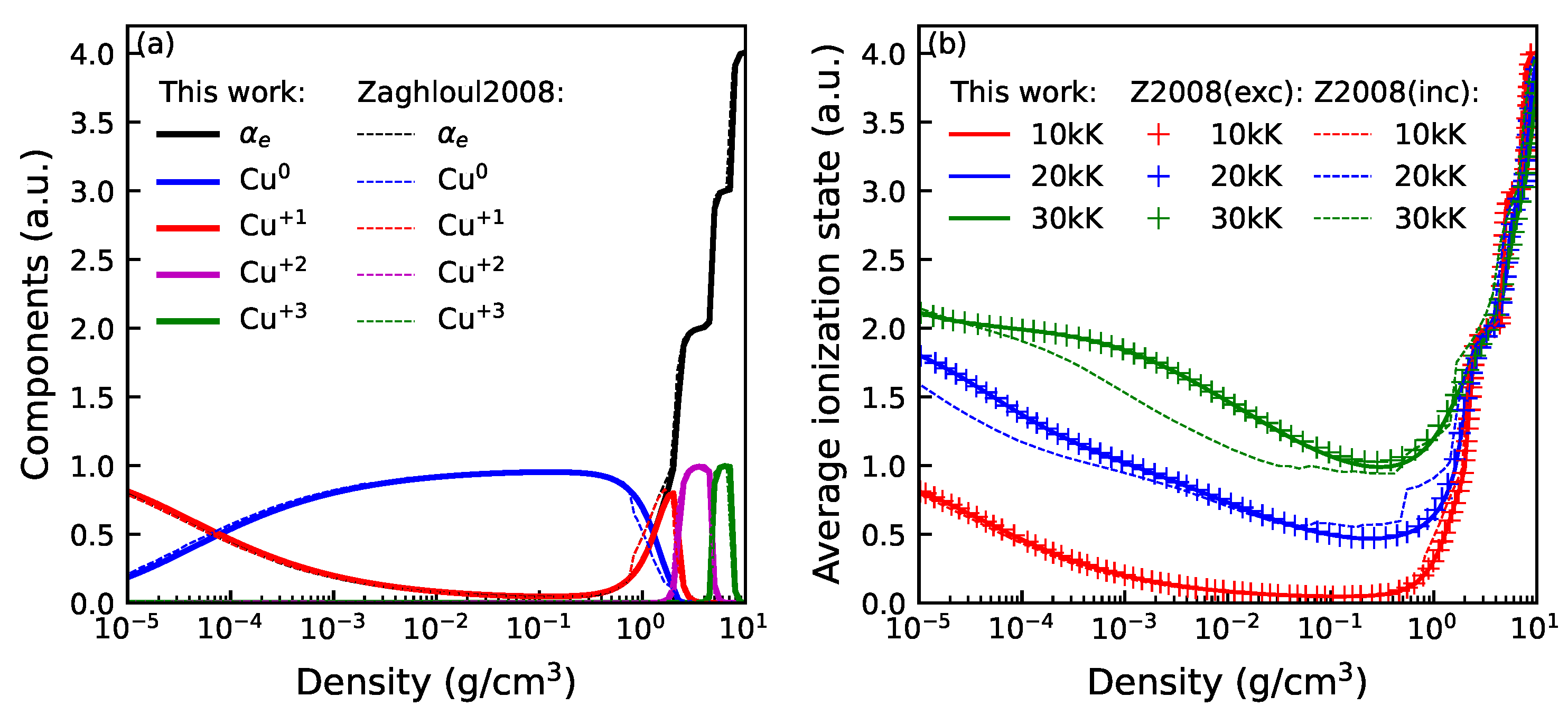
3.1. Validation of Saha Equation Solver

In principle, it is best to justify the application of the model to Ta by comparisons with experimental measurements. In reality, however, research on tantalum has been relatively scarce. To the best of our knowledge, the only available experimental data of electrical conductivity for Ta are those reported by DeSilva and Vunni [8], which will be discussed in Section 3.4. Additionally, there has not been any reported measurement on the ionization states of a Ta plasma. In lieu of experimental data, we argue that the validation of the model for Ta can be justified by its wide applicability to a variety of elements. For example, it has been utilized to study low-Z plasmas such as aluminium [24], medium-Z plasmas such as iron, nickel [25], and copper [12], and high-Z plasmas such as tungsten [20]. In all these studies, the model has achieved either qualitative or quantitative agreement with experimental data, indicating its applicability within a wide range of Z. Therefore, we believe that applying the model for Ta is reasonable.

To validate the nonideal Saha equation solver utilized in this study, the detailed compositions of copper (Cu) plasma at T = 10,000 K have been calculated as functions of density, as shown in Figure 1a. In our calculations, ionization states up to $i=Z_{\mathrm{Cu}}$ are considered. It is found that for most densities the abundance of the ith state ($i>3$) is orders of magnitude lower than that of the first three ones, so we only plot states up to Cu⁺³ for clarity. Excellent agreement has been achieved between the results of this study and those of Ref. [12], except for certain minor discrepancies within 0.5 < $\rho$ < 1 g/cm³. Namely, ${\alpha }_0$ and ${\alpha }_1$ from Ref. [12] exhibit a more abrupt decrease and increase, respectively. In contrast, the variations in both ${\alpha }_0$ and ${\alpha }_1$ obtained in this study with respect to density are more gradual. Similar trends are also observed at T = 20,000 and 30,000 K across broader density ranges.

Such discrepancies arise from the exclusion of electronic excitation states in the partition function calculations [12]. However, the introduced errors in ${\alpha }_i$s are generally less than ∼10%, and remain less than ∼50% even under high-temperature conditions. In Figure 1b, we also explicitly compare ${\alpha }_e$s with and without electronic excitation states at T = 10,000, 20,000, and 30,000 K. It is clear that even at 30,000 K the errors between ${\alpha }_e$s are still less than ∼30%. Therefore, the overall trends and interpretations of the results will not be qualitatively altered. These effects also manifest in the electrical conductivity, as discussed in the following section.

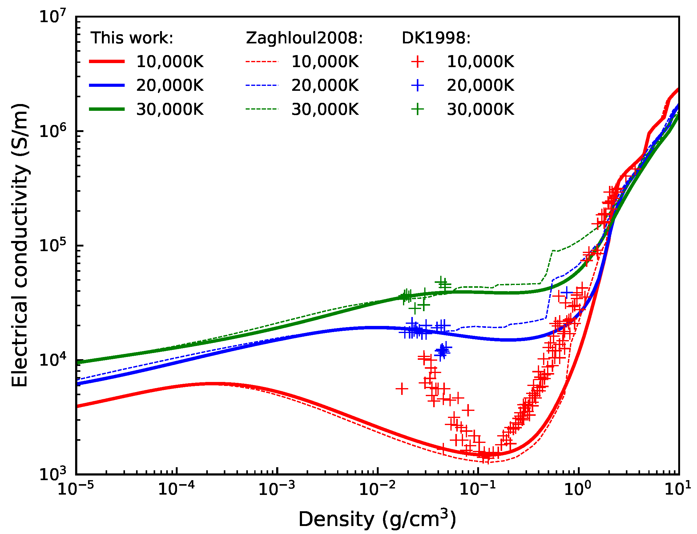
3.2. Validation of Electrical Conductivity Calculation

To validate the electrical conductivity model employed in this study, the isotherms of $\sigma (\rho ;T)$ for Cu plasma at T = 10,000, 20,000, and 30,000 K are calculated, as shown in Figure 2. Good agreement with the results of Zaghloul [12] confirms the overall accuracy of the model. Discrepancies primarily occur within 0.1 < $\rho$ < 2 g/cm³, and are more pronounced at elevated temperatures of 20,000 K and 30,000 K. At these moderate densities, the predominant contribution to the total electrical conductivity arises from the electron–neutral collision term ${\sigma }_{en}$, which is inversely proportional to ${\alpha }_0$ according to Equation (15). As discussed in Section 3.1, the abrupt decrease in ${\alpha }_0$ due to the inclusion of electronic excitation states leads to an increase in ${\sigma }_{en}$ as well as $\sigma$. However, the discrepancies in $\sigma$ remain in a relatively narrow density range, and the overall applicability of the model is not affected.

The results of the model are further compared with the experimental data of DeSilva and Katsourous [26] (see plus symbols in Figure 2). At T = 10,000 K and 0.02 ≲ $\rho$ ≲ 2 g/cm³, both theoretical and experimental results exhibit qualitatively similar trends, with a minimum value of approximately ${10}^3$ S/m at $\rho$≈ 0.1∼0.2 g/cm³. However, the calculations significantly underestimate $\sigma$ by several times for $\rho$ < 0.1 g/cm³. At T = 20,000 and 30,000 K, there is good agreement between the experimental and theoretical results for 0.02 g/cm³ < $\rho$ < 0.05 g/cm³, except for a slight overestimation of $\sigma$ at $T=20,000$ K and $\rho$ ≈ 0.05 g/cm ³. Compared to other methods, the model of this study has obtained better agreement with experimental data than the Burgess model [27]. It is worth noting that the modified Lee–More (MLM) model [21] can provide even better results. In fact, our model follows the same accurate treatment of electron–neutral collisions as MLM, but lacks the smooth blend between Saha and Thomas–Fermi ionization equilibriums adopted in MLM. Furthermore, the accuracy of the calculations could be enhanced with more precise atomic parameters.

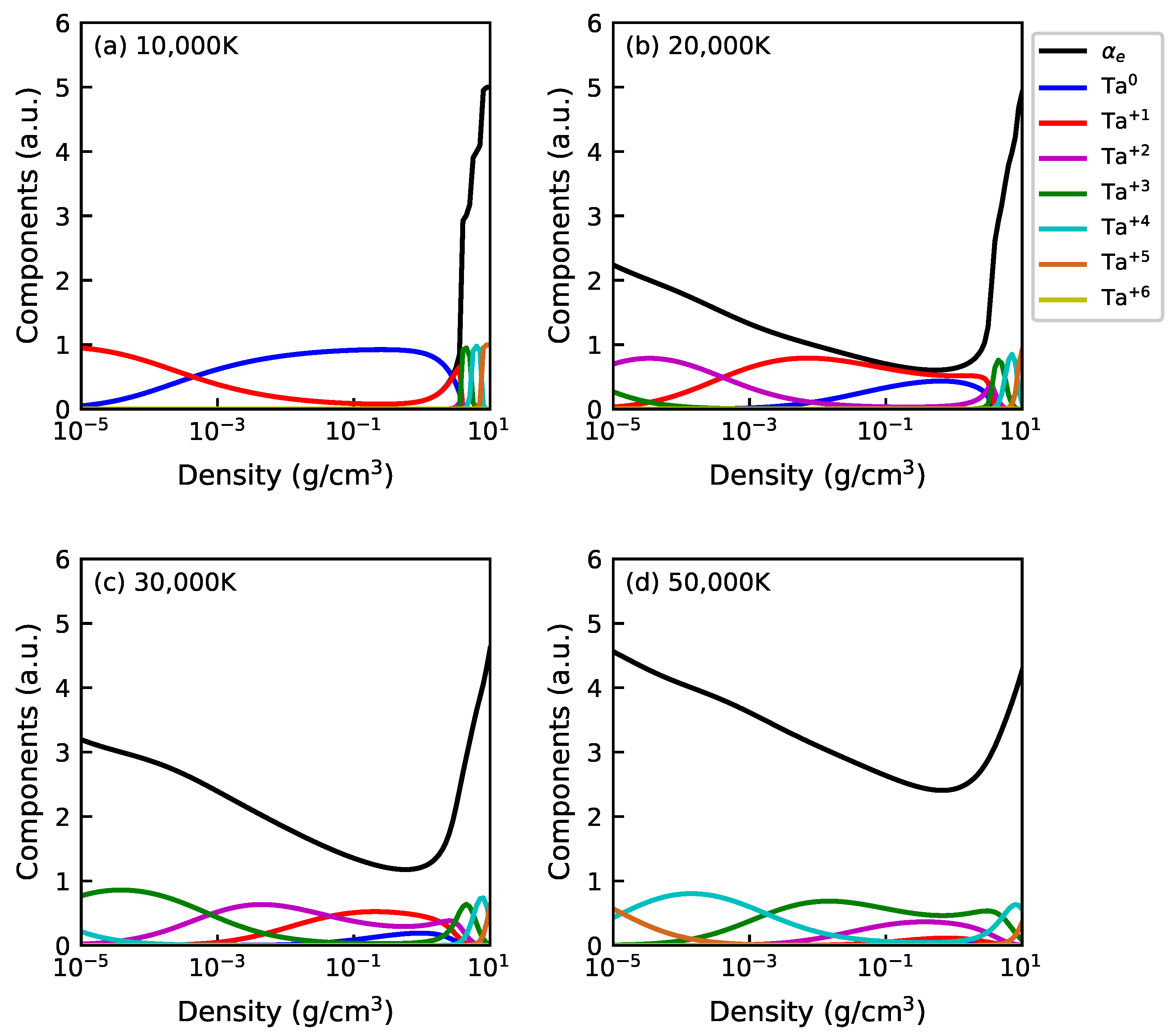
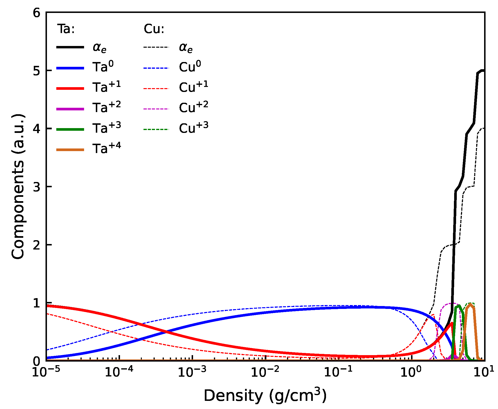
3.3. Ionization States of Tantalum Plasmas

After validating our theoretical model and numerical algorithm, we proceed to calculate the detailed composition of tantalum plasma as a function of density at various temperatures, specifically T = 10,000 K, 20,000 K, 30,000 K, and 50,000 K, as illustrated in Figure 3. Ionization states up to $i=Z_{\mathrm{Ta}}$ are included in our calculations. Similar to the case of Cu, the abundance of the ith state (i > 6) is negligible, and only the first six ionization states are plotted for clarity. Several characteristics of the detailed composition of Ta plasma are observed. Firstly, the average ionization states ${\alpha }_e$s exhibit a minimum value in the vicinity of $\rho$∼1 g/cm³. At low densities, such as $\rho$ = 10⁻⁵ g/cm³, ${\alpha }_e$ shows a roughly linear dependence on temperature T, increasing from 1 at 10,000 K to approximately 4.5 at 50,000 K. In contrast, at high densities near 10 g/cm³, ${\alpha }_e$ remains around 5 and is insensitive to temperature increase. This feature can be attributed to variations in ionization compositions. At high densities, higher ionization states dominate due to the reduction in ionization energies, even at lower temperatures. In particular, the Ta⁺³ to Ta⁺⁵ species constitute the majority of the ionization composition at T = 10,000∼50,000 K. Consequently, the average ionization state remains relatively stable with respect to temperature changes. On the other hand, the ionization composition at low densities undergoes significant changes as T increases. Specifically, the Ta⁺¹ species dominates at 10,000 K, followed by the Ta⁺² species at 20,000 K, and so forth. This successive increase in the charge state of the dominant species results in a linear temperature dependence of ${\alpha }_e$.

Secondly, it is intriguing to compare the average ionization states and detailed ionization compositions of tantalum and copper plasmas at identical densities and temperatures to evaluate the effects of elemental species, as shown in Figure 4. It is noteworthy that the different ionization states of the two elements exhibit remarkably similar compositional behaviors. In particular, the Ta⁺¹ and Cu⁺¹, Ta⁺³ and Cu⁺², and Ta⁺⁴ and Cu⁺³ species demonstrate qualitatively similar density-dependent relationships. These similarities among the various ionization states of different elements can be attributed to the comparable ionization energies of the corresponding states. The ionization energies of Cu⁰, Cu⁺¹, and Cu⁺² are 7.73 eV, 20.29 eV, and 36.84 eV, respectively. Similarly, the ionization energies of Ta⁰, Ta⁺², and Ta⁺³ are 7.55 eV, 23.1 eV, and 35.0 eV, respectively. The ionization energies of these two elements are closely aligned, resulting in the similar ionization compositions observed.

3.4. Electrical Conductivity of Tantalum Plasmas

As demonstrated in Equation (14), both electron–ion and electron–neutral collisions contribute to electrical conductivity. In low-density regions, the plasma is in a state of complete thermal ionization due to minimal recombination. Consequently, electron–ion collisions make the primary contribution to electrical conductivity, resulting in an approximately linear dependence of $\sigma$ on $ln\rho$ (see Figure 5). In high-density regions, the average ionization state of the plasma increases significantly due to pressure ionization, and electron–ion collisions continue to dominate in the calculations of electrical conductivity.

In intermediate-density regions, the effects of thermal ionization and recombination compete with one another. At low temperatures, the thermal ionization effect can be suppressed by the recombination process, resulting in a significantly low average ionization state (see Figure 3). In this scenario, electrical conductivity is primarily determined by electron–neutral collisions. On the other hand, at sufficiently high temperatures the recombination process may not be strong enough to counteract the thermal ionization effect, so the average ionization state decreases mildly and remains at a relatively high level. In this case, the contribution of electron–neutral collisions is not necessarily greater than that of electron–ion collisions.

Another crucial parameter in electrical conductivity calculation is the electron–neutral momentum transfer cross-section. As indicated in Equation (15), ${\sigma }_{en}$ is inversely proportional to ${\overline{Q}}_{en}$. Typically, in the intermediate-density region and at relatively low temperatures where electron–neutral collisions are significant, ${\sigma }_{en}$ is smaller than ${\sigma }_{ei}$. According to Equation (14), $\sigma$ tends to approximate the smaller value within $({\sigma }_{en},{\sigma }_{ei})$. Consequently, the effects of electron–neutral collisions become evident (see Figure 5). However, if under certain conditions ${\overline{Q}}_{en}$ becomes excessively small, the resulting ${\sigma }_{en}$ can be large. If ${\sigma }_{en}$∼${\sigma }_{ei}$, the aforementioned intermediate-density effect can be significantly diminished.

To illustrate the effect of ${\overline{Q}}_{en}$, the isotherms of the calculated electrical conductivity of tantalum plasma $\sigma (\rho ;T)$ with varying values of ${\overline{Q}}_{en}$ are presented in Figure 6. For instance, at T = 10,000 K and ${\overline{Q}}_{en}$ = 1.5 × 10⁻²⁰ m², the intermediate-density range is relatively narrow, spanning from approximately 0.1 g/cm³ to 4 g/cm³. The reduction in electrical conductivity due to electron–neutral collisions is merely a factor of 2 to 3. A comparison with Figure 5 suggests that within this density range, both ${\sigma }_{en}$ and ${\sigma }_{ei}$ significantly contribute to these characteristics. As ${\overline{Q}}_{en}$ increases to 1.5 × 10⁻¹⁸ m², the range of intermediate density broadens, and the reduction in electrical conductivity can exceed an order of magnitude.

In Figure 6, we present the experimental measurements conducted by DeSilva and Vunni [8] (gray open squares). Since they measured internal energy rather than temperature for each data point, establishing a direct connection between these data points and the isotherms is not straightforward; thus, a specific equation-of-state model is required. However, it is reasonable to assert that the temperatures corresponding to these data points fall within the range of 10,000 K to 50,000 K (see, for example, Ref. [9]). Consequently, adjusting the value of ${\overline{Q}}_{en}$ to ensure that the experimental data points are entirely encompassed within the calculated isotherms can serve as a method for estimating the average electron–neutral momentum transfer cross-section.

It has also been observed that for densities around 10 mg/cm³ and sufficiently small values of ${\overline{Q}}_{en}$, the temperature dependence of electrical conductivity can exhibit non-monotonic behavior. As illustrated in Figure 7, for ${\overline{Q}}_{en}$ = 1.5 × 10⁻²⁰ m², the electrical conductivity decreases as the temperature rises from 10,000 K to 20,000 K, and then increases with further temperature increases. In contrast, for larger values of ${\overline{Q}}_{en}$, electrical conductivity $\sigma$ increases monotonically with temperature T.

Recently, it has been proposed that under-critical foams can be utilized in ICF [28]. One significant application of foam materials involves lining the walls of the hohlraum with a low-density tantalum oxide foam to mitigate the detrimental effects of inward wall motion within the hohlraum [4]. Although the density of the lining foam is typically controlled to remain under-critical to ensure the penetration of the incident laser beam, the absorption of laser energy by the foam plasma has not yet been evaluated. Once the electrical conductivity is calculated, the absorption of laser energy can be assessed using the Drude model [29]:

$$n_r^2-n_i^2=1-{\sigma }_0{\displaystyle \frac{\nu }{{\epsilon }_0({\omega }^2+{\nu }^2)}},2n_r{n}_i={\sigma }_0{\displaystyle \frac{{\nu }^2}{{\epsilon }_0\omega ({\omega }^2+{\nu }^2)}},\alpha =2{\displaystyle \frac{\omega }{c}}{n}_i,$$

(19)

where ${\sigma }_0$ is the direct current (DC) electrical conductivity, and $n_r$ and $n_i$ represent the real and imaginary components of the complex index of refraction, respectively. $\omega$ denotes the laser frequency, c is the speed of light, $\alpha$ is the absorption coefficient, and $\nu =1/\tau$ with $\tau$ is the electron relaxation time. The typical density of foam ranges from approximately 10 to 100 mg/cm³, placing it within the intermediate-density region discussed earlier. In this region, the electron relaxation time can be approximated as described in Ref. [30]:

$${\displaystyle \frac{1}{\tau }}\approx {\displaystyle \frac{1}{{\tau }_{en}}}=n_0{v}_e{\overline{Q}}_{en},$$

(20)

where $n_0$ represents the neutral density and $v_e$ denotes the electron thermal velocity. For 10 ≲ $\rho$ ≲ 100 mg/cm³ and for an NIF laser wavelength of 351 nm [31], the electrical conductivity of Ta is approximately 10³ S/m, in contrast to its value at normal density, which exceeds 10⁵ S/m. As a result, the absorption coefficient $\alpha$ can be reduced by about two orders of magnitude. Therefore, laser absorption in the under-critical tantalum foam plasma is weak, rendering its effect on laser energy deposition into the hahlraum negligible.

4. Conclusions

This study utilizes a theoretical model to calculate the ionization states and electrical conductivity of tantalum plasma. The calculated average ionization state of tantalum plasma exhibits a minimum value at a density of 1 g/cm³. At low densities, the ionization state increases linearly with temperature, while at high densities it remains relatively stable due to pressure ionization effects. The ionization compositions of tantalum and copper plasmas display similar trends at corresponding ionization states, which can be attributed to their comparable ionization energies.

The electrical conductivity of tantalum plasma is significantly influenced by electron–neutral collisions in the intermediate-density region. The conductivity demonstrates a non-monotonic temperature dependence at low densities and small electron–neutral momentum transfer cross-sections. Calibration with experimental data indicates that the average electron–neutral momentum transfer cross-section can be estimated to enhance the accuracy of conductivity calculations. For under-critical tantalum foam plasmas, the electrical conductivity is low (approximately 10³ S/m), resulting in weak laser absorption. This suggests that laser energy deposition in hohlraums lined with tantalum oxide foam is negligible, thereby validating its use in ICF applications.

References

1. Bayu-Aji, L.B.; Engwall, A.M.; Bae, J.H.; Baker, A.A.; Beckham, J.L.; Shin, S.J.; Lepro Chavez, X.; McCall, S.K.; Moody, J.D.; Kucheyev, S.O. Sputtered Au-Ta films with tunable electrical resistivity. J. Phys. D Appl. Phys. 2021, 54, 075303. [Google Scholar] [CrossRef]
2. Frederick, C.A.; Forsman, A.C.; Hund, J.F.; Eddinger, S.A. Fabrication of Ta2O5 aerogel targets for radiation transport experiments using thin film fabrication and laser processing. Fusion Sci. Technol. 2009, 55, 499–504. [Google Scholar] [CrossRef]
3. Baker, A.A.; Engwall, A.M.; Bayu-Aji, L.B.; Bae, J.H.; Shin, S.J.; Moody, J.D.; Kucheyev, S.O. Tantalum suboxide films with tunable composition and electrical resistivity deposited by reactive magnetron sputtering. Coatings 2022, 12, 917. [Google Scholar] [CrossRef]
4. Bhandarkar, S.; Baumann, T.; Alfonso, N.; Thomas, C.; Baker, K.; Moore, A.; Larson, C.; Bennett, D.; Sain, J.; Nikroo, A. Fabrication of low-density foam liners in hohlraums for NIF targets. Fusion Sci. Technol. 2018, 73, 194–209. [Google Scholar] [CrossRef]
5. Berger, R.L.; Arrighi, W.; Chapman, T.; Dimits, A.; Banks, J.W.; Brunner, S. The competing effects of wave amplitude and collisions on multi-ion species suppression of stimulated Brillouin scattering in inertial confinement fusion hohlraums. Phys. Plasmas 2023, 30, 042715. [Google Scholar] [CrossRef]
6. Zhernokletov, M.V.; Simakov, G.V.; Sutulov, Y.N.; Trunin, R.F. Expansion isentropes of aluminum, iron, molybdenum, lead, and tantalum. High Temp. 1995, 33, 40–43. [Google Scholar]
7. Miljacic, L.; Demers, S.; Hong, Q.J.; van de Walle, A. Equation of state of solid, liquid and gaseous tantalum from first principles. Calphad 2015, 51, 133–143. [Google Scholar] [CrossRef]
8. DeSilva, A.W.; Vunni, G.B. Electrical conductivity of dense Al, Ti, Fe, Cu, Mo, Ta, and W plasmas. Phys. Rev. E 2011, 83, 037402. [Google Scholar] [CrossRef]
9. Apfelbaum, E.M. The pressure, internal energy, and conductivity of tantalum plasma. Contrib. Plasma Phys. 2017, 57, 479–485. [Google Scholar] [CrossRef]
10. Harris, G.M.; Roberts, J.E.; Trulio, J.G. Equilibrium properties of a partially ionized plasma. Phys. Rev. 1960, 119, 1832–1841. [Google Scholar] [CrossRef]
11. Zaghloul, M.R. Reduced formulation and efficient algorithm for the determination of equilibrium composition and partition functions of ideal and nonideal complex plasma mixtures. Phys. Rev. E 2004, 69, 026702. [Google Scholar] [CrossRef]
12. Zaghloul, M.R. A simple theoretical approach to calculate the electrical conductivity of nonideal copper plasma. Phys. Plasmas 2008, 15, 042705. [Google Scholar] [CrossRef]
13. Wang, W.Z.; Rong, M.Z.; Yan, J.D.; Murphy, A.B.; Spencer, J.W. Thermophysical properties of nitrogen plasmas under thermal equilibrium and non-equilibrium conditions. Phys. Plasmas 2011, 18, 113502. [Google Scholar] [CrossRef]
14. Das, M. Transition energies and polarizabilities of hydrogen like ions in plasma. Phys. Plasmas 2012, 19, 092707. [Google Scholar] [CrossRef]
15. Ecker, G.; Kröll, W. Lowering of the ionization energy for a plasma in thermodynamic equilibrium. Phys. Fluids 1963, 6, 62–69. [Google Scholar] [CrossRef]
16. Stewart, J.C.; Pyatt, K.D., Jr. Lowering of ionization potentials in plasmas. Astrophys. J. 1966, 144, 1203–1211. [Google Scholar] [CrossRef]
17. Kramida, A.; Ralchenko, Y.; Reader, J.; Team, N.A. NIST Atomic Spectra Database. 2024. Available online: https://physics.nist.gov/asd (accessed on 10 April 2025).
18. Trayner, C.; Glowacki, M.H. A new technique for the solution of the Saha equation. J. Sci. Comput. 1995, 10, 139–149. [Google Scholar] [CrossRef]
19. Kim, D.K.; Kim, I. Calculation of ionization balance and electrical conductivity in nonideal aluminum plasma. Phys. Rev. E 2003, 68, 056410. [Google Scholar] [CrossRef]
20. Fu, Z.; Jia, L.; Sun, X.; Chen, Q. Electrical conductivity of warm dense tungsten. High Eenergy Density Phys. 2013, 9, 781–786. [Google Scholar] [CrossRef]
21. Desjarlais, M.P. Practical improvements to the Lee-More conductivity near the metal-insulator transition. Contrib. Plasma Phys. 2001, 41, 267–270. [Google Scholar] [CrossRef]
22. Spitzer, L., Jr.; Härm, R. Transport phenomena in a completely ionized gas. Phys. Rev. 1953, 89, 977–981. [Google Scholar] [CrossRef]
23. Zollweg, R.J.; Liebermann, R.W. Electrical conductivity of nonideal plasmas. J. Appl. Phys. 1987, 62, 3621–3627. [Google Scholar] [CrossRef]
24. Zaghloul, M.R. On the calculation of the electrical conductivity of hot dense nonideal plasmas. Plasma Phys. Rep. 2020, 46, 574–586. [Google Scholar] [CrossRef]
25. Kim, D.K.; Kim, I. Electrical conductivities of nonideal iron and nickel plasmas. Contrib. Plasma Phys. 2007, 47, 173–176. [Google Scholar] [CrossRef]
26. DeSilva, A.W.; Katsourous, J.D. Electrical conductivity of dense copper and aluminum plasmas. Phys. Rev. E 1998, 57, 5945–5951. [Google Scholar] [CrossRef]
27. Kim, K.; Jang, S. System modeling and simulation of flyer acceleration and explosive detonation in exploding foil initiator. AIP Adv. 2023, 13, 065329. [Google Scholar] [CrossRef]
28. Limpouch, J.; Tikhonchuk, V.; Renner, O.; Agarwal, S.; Burian, T.; Cervenka, J.; Dostal, J.; Dudzak, R.; Ettel, D.; Gintrand, A.; et al. Laser interaction with undercritical foams of different spatial structures. Matter Radiat. Extrem. 2025, 10, 017402. [Google Scholar] [CrossRef]
29. Wu, B.; Shin, Y.C. Absorption coefficient of aluminum near the critical point and the consequences on high-power nanosecond laser ablation. Appl. Phys. Lett. 2006, 89, 111902. [Google Scholar] [CrossRef]
30. Lee, Y.T.; More, R.M. An electron conductivity model for dense plasmas. Phys. Fluids 1984, 27, 1273–1286. [Google Scholar] [CrossRef]
31. Spaeth, M.L.; Manes, K.R.; Kalantar, D.H.; Miller, P.E.; Heebner, J.E.; Bliss, E.S.; Spec, D.R.; Parham, T.G.; Whitman, P.K.; Wegner, P.J.; et al. Description of the NIF laser. Fusion Sci. Technol. 2016, 69, 25–145. [Google Scholar] [CrossRef]
Figure 1. (a) Average ionization state and detailed plasma composition for copper plasma at various densities at a temperature of 10,000 K (solid curves). For comparison, the results from Zaghloul [12] (dashed curves) are also presented. (b) Isotherms of the average ionization states of copper plasma at temperatures of 10,000 K (red solid), 20,000 K (blue solid), and 30,000 K (green solid). For reference, the results from Ref. [12], which exclude (plus symbols) and include (dashed curves) electronically excited states, are also shown.
Plasma 08 00016 g001
Figure 2. Isotherms of the calculated electrical conductivity of copper in this study (solid bold curves) at temperatures of 10,000 K (red), 20,000 K (blue), and 30,000 K (green). For comparison, the theoretical results from Zaghloul [12] (dashed thin curves) and the experimental measurements by DeSilva and Katsourous [26] (plus symbols) are also presented.
Plasma 08 00016 g002
Figure 3. Average ionization states and detailed ionization compositions of tantalum plasma at different densities at (a) 10,000 K, (b) 20,000 K, (c) 30,000 K, and (d) 50,000 K.
Plasma 08 00016 g003
Figure 4. Comparison of the average ionization states and detailed ionization compositions of Ta (solid curves) and Cu (dashed curves) plasmas at different densities at 10,000 K.
Plasma 08 00016 g004
Figure 5. Isotherm of electrical conductivity associated with electron–neutral collisions σ e n for Ta plasma at 10,000 K, calculated using various average electron–neutral momentum transfer cross-sections (solid bold curves). For comparison, the isotherm of σ e n for Cu plasma (black solid thin curve) as well as the isotherms of electrical conductivity related to electron–ion collisions σ e i for both Ta (red dashed curve) and Cu (black dashed curve) are also included.
Plasma 08 00016 g005
Figure 6. Isotherms of the calculated electrical conductivity of Ta as a function of density and temperature, with varying average electron–neutral momentum transfer cross-sections: (a) Q ¯ e n = 1.5 × 10⁻²⁰ m2, (b) Q ¯ e n = 1.5 × 10⁻¹⁹ m2, and (c) Q ¯ e n = 1.5 × 10⁻¹⁸ m2. For reference, the experimental measurements by DeSilva and Vunni [8] (gray open squares) are also included. Notice that the conductivity was measured as a function of relative internal energy rather than temperature, and the estimated temperatures were approximately between 20,000 K and 30,000 K [8,9].
Plasma 08 00016 g006
Figure 7. Electrical conductivity of tantalum plasma as a function of temperature, at a density of 1 mg/cm3, calculated using various values of the average electron–neutral momentum transfer cross-section.
Plasma 08 00016 g007
Disclaimer/Publisher’s Note: The statements, opinions and data contained in all publications are solely those of the individual author(s) and contributor(s) and not of MDPI and/or the editor(s). MDPI and/or the editor(s) disclaim responsibility for any injury to people or property resulting from any ideas, methods, instructions or products referred to in the content.