Thermoresponsive Effects in Droplet Size Distribution, Chemical Composition, and Antibacterial Effectivity in a Palmarosa (Cymbopogon martini) O/W Nanoemulsion

Abstract

The design of emulsions at the nanoscale is a significant application of nanotechnology. For spherical droplets and a given volume of dispersed phase, the nanometre size of droplets inversely increases the total area, $A={\displaystyle \frac{3V}{r}}$, allowing greater contact with organic and inorganic materials during application. In topical applications, not only is cell contact increased, but also permeability in the cell membrane. Nanoemulsions typically achieve kinetic stability rather than thermodynamic stability, so their commercial application requires reasonable resistance to flocculation and coalescence, which can be affected by temperature changes. Therefore, their thermoresponsive characterisation becomes relevant. In this work, we analyse this response in an O/W nanoemulsion of Palmarosa for antibacterial purposes that has already shown stability for one year at controlled room temperature. We now study hysteresis processes and the behaviour of the statistical distribution in droplet size by Dynamic Light Scattering, obtaining remarkable stability under temperature changes up to 50 °C. This includes a maintained chemical composition observed using Fourier Transform Infrared Spectroscopy and the preservation of antibacterial properties analysed through optical density tests on cultures and the Spread-Plate technique for bacteria colony counting. We obtain practically closed hysteresis curves for some tracers of droplet size distributions through controlled thermal cycles between 10 °C and 50 °C, exhibiting a non-linear behaviour in their distribution. In general, the results show notable physical, chemical, and antibacterial stability, suitable for commercial applications.

1. Introduction

As technology advances, nanoscale products have emerged as a novel approach that provides new and enhanced properties to materials. Nanoscale products have garnered interest because of their higher surface-to-volume ratio, which increases the likelihood that the material will come into contact with various substances. Nanoemulsions (NEs) exemplify how size reduction can enhance the effects of the materials that they comprise [1]. In recent years, the application of NEs has increased significantly in fields such as pharmaceutical, food, agriculture, cosmetics, and materials industries, due to the potential advantages they offer over conventional emulsions [2,3,4]. They have been used to improve the appearance, stability, controlled release, and bioavailability of various products [2]. NEs consist of two immiscible phases, with a dispersed phase stabilised in a continuous phase by an emulsifier.

Emulsified systems have various applications in the chemical industries. Composed of immiscible substances that tend to separate over time, they are commonly stabilised using emulsifiers to delay phase separation. The application of essential oils (EOs) in an emulsified form has been envisaged as a simple and economical means to limit the effects of pathogens (bacteria and fungi) in different forms [5,6,7]. EOs are a mixture of volatile compounds extracted from different parts of aromatic plants by distillation [8,9]. Despite the presence of 20 to 60 bioactive compounds in EOs, only two or three in higher concentrations are responsible for the characteristic properties of EOs [10].

Whether in foods or applied topically to the skin, preventive effects have been observed against the proliferation of these pathogens. For example, EOs of Cymbopogon martini (commonly known as Palmarosa) have been extensively studied due to their antimicrobial properties against microorganisms and their wide application in the cosmetic, food, and pharmaceutical industries [8,10,11,12,13]. Geraniol is the main monoterpene compound present in Palmarosa EO, which exhibits antimicrobial properties. Its lipophilicity allows it to permeabilise cell membranes, causing functional and structural damage to the cell [14]. However, when oil-in-water (O/W) emulsions have microsized droplets, the effect of antibacterial components in the EOs is markedly reduced, particularly because of their difficult access to the EOs through the pathogens’ cell membranes. In addition, these emulsions generally have limited lifespans as a result of separation of their components by coalescence or flocculation.

An advisable solution is to achieve droplet sizes in the continuous phase at the nanoscale, either by spontaneous or induced means. Droplets of this scale are usually less susceptible to phenomena such as coalescence and flocculation, maintaining thermodynamic or kinetic stability for longer periods [15,16,17]. Furthermore, the application of these compounds on the nanoscale increases the permeability of the cell membrane [18,19]. In particular, the improved bioavailability of certain substances with organic tissues or even cells, through an increased contact area, has substantial applicability and value. In contemporary classification, an NE is an emulsion with droplets at the nanoscale induced by applying energy, commonly achieving high kinetic stability in droplet size rather than thermodynamic stability [16,20]. In recent years, interest has grown in the manufacture and improvement of NEs due to their efficacy, transport, and the bioavailability of their dispersed phase compared to conventional emulsions at the microscale [2]. When induced methods are necessary, the kinetic stability can still be extended by a surfactant that creates a pronounced relative minimum in free energy by reducing interfacial stress [21,22]. This stability is still susceptible to temperature fluctuations, which should be considered for commercial applications because their ability to interact with cell membranes and deposit substances efficiently is due to the predominant droplet size (around 1–100 nm). Although their induced fabrication methods require a large amount of energy [21,23,24,25], there are controlled methods such as ultrasound that do not require a large amount of energy and can reduce overheating in EO, preventing loss of antibacterial properties by altering their characteristic chemical components when properly controlled [26,27]. However, temperature fluctuations present in commercial applications could introduce similar effects, altering not only the chemical composition but also the initial characterisation of the droplet size, thus doubly reducing its effectiveness.

This work analyses some thermoresponsive effects on a demonstrated kinetically stable O/W NE based on Palmarosa EO [28]. Commercialisation requires ensuring that these NEs have sufficient durability, thereby preserving the properties for which they were originally developed, thus achieving enhanced effects for manufacturing purposes. In particular, we are interested in hysteresis, a phenomenon in which a material retains some of its properties in the absence of the original stimulus that generated it, triggered by a cyclical change in one or more of its parameters or additional properties. In this sense, we can speak of hysteresis cycles in the droplet size distributions of emulsions, for example, due to variations in their temperature depending on the thermal history of the system when an emulsion is subjected to heating and cooling cycles. This is due to variations in surface tension, viscosity of the continuous medium, or redistribution of the surfactant. These changes are not always reversible, which generates an open cycle. Thus, when an emulsion is heated, the droplets can coalesce and increase in size, but when cooled, they will not necessarily return to their original size due to the formation of more stable structures. This phenomenon is important in industrial or commercial applications where emulsion stability is crucial because of its nanoscale properties. Understanding how temperature affects the droplet size distribution can help design more efficient processes and more stable products.

Thus, the effect of temperature changes on the kinematic equilibrium can become a limitation since heating promotes coalescence and flocculation, potentially leading to hysteresis cycles. This phenomenon is not always irreversible around the point of kinematic equilibrium. It is therefore important to delimit the thermoresponsive effect on the droplet size of the NE and its polydispersity. It is also crucial to quantify the impact of temperature fluctuations on the preservation of antibacterial properties in the associated EO chemical components. This research aimed to analyse the thermal response in the polydispersity of a Palmarosa (Cymbopogon martini) NE with an EO concentration of 5%, which was previously reported to have a stable droplet size over a period of one year [28].

Palmarosa oil was selected among other EOs due to its antimicrobial effects and affordability [8,10,11,12,13,29]. The NE being considered has shown kinematic stability in its droplet size for as long as one year, without special storage conditions other than darkness at room temperature [28]. It has also exhibited enhanced antibacterial properties because of its nanoscale droplet size. In the current research, the NE is exposed to mild temperature changes, thus tracking such a stability phenomenon under extended thermoresponsivity tests. Furthermore, it is desired to observe whether a hysteresis phenomenon is present in the NE through heating and cooling processes, their quantitative extent, and how it possibly affects the chemical composition and potentially its antibacterial features. In this sense, the interest in improving its stability and avoiding the effects of flocculation and coalescence is important, particularly to address thermoresponsivity effects in extreme conditions of daily use, such as topical application, by reproducing the typical handling in commercial uses.

The organisation of this work is as follows. Section 2 outlines the Materials and Methods. The Section 3 presents the main outcomes for the physical response under temperature changes, particularly those related to droplet size distribution fluctuations and hysteresis. Section 4 reports a comparative analysis of the chemical composition of NE between the initial and final stages of the previous physical thermoresponsive tests. Section 5 discusses the preserved antibacterial properties using the Spread-Plate (SP) diffusion method and measuring the optical density (OD) of biological cultures (measured as absorbance in the current work). Conclusions are included in the Section 6.

2. Materials and Methods

This section presents the Materials and Methods to compare the droplet size distribution, chemical composition, and antibacterial features before and after thermoresponsive tests. Dynamic Light Scattering (DLS) was used as a central method to track the droplet size distribution through heating and cooling cycles. A comparative preserved antibacterial effectiveness against some Gram-positive and Gram-negative bacteria was investigated between NEs exposed and not exposed to heating–cooling cycles, together with a follow-up of some relevant chemical components. The complete dataset for this research is public [30]. Thus, the particular objectives of the research were the following:

(1)

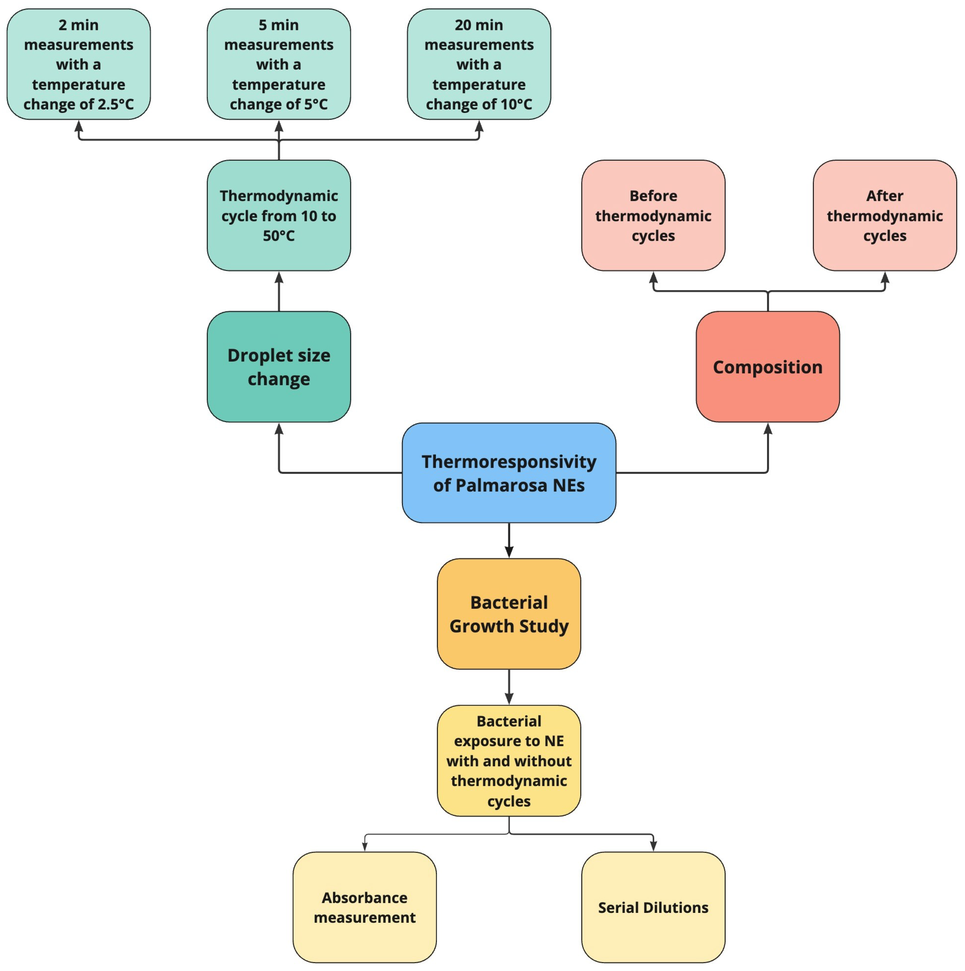
Analyse the thermoresponsive droplet size behaviour for a stable one-year 5% O/W NE of Palmarosa under heating and cooling cycles ranging from 10 °C to 50 °C.

(2)

Determine whether, under thermal cycles, there exists a hysteresis process for the characteristic and average diameters in the droplet size distribution.

(3)

Compare whether an NE exposed to repeated thermal cycles of heating and cooling in the range of 10 °C to 50 °C exhibits changes in its chemical composition.

(4)

Compare whether an NE exposed to repeated thermal cycles of heating and cooling in the range of 10 °C to 50 °C has altered antibacterial effectiveness.

2.1. Materials

2.1.1. Essential Oils, Surfactant, and Continuous Phase

For this study, a cosmetic-grade Cymbopogon martini EO with a CAS number of 8014-19-5 was obtained from a local supplier (Droguería Cosmopolita in Mexico City, Mexico). Distilled water was used as the continuous phase. Among several possible surfactants, Eumulgin was chosen because it is a safe substance for human use with a daily maximum exposure of 9 mg according to the FDA [31]. Both distilled water and cosmetic grade Eumulgin (CAS 61788-85-0) were purchased from CTR Scientific (Mexico City, Mexico), a national supplier of laboratory equipment and chemical reagents.

2.1.2. Bacterial Strains

To ensure the efficacy of the NEs as antibacterial agents even after thermal cycles, we performed a kinetic bacterial growth study. Four different bacterial strains of high medical and pharmaceutical interest were selected to evaluate their response when exposed to the NEs. Bacillus subtilis and Staphylococcus aureus were chosen as two representative and relevant Gram-positive bacteria, while Escherichia coli and Salmonella spp. were chosen as Gram-negative bacteria. These bacteria are of relevance to clinical studies because of their adverse effects on the body and their recent development of bacterial resistance to different types of antibiotics. The samples were obtained as clinical isolates from the Autonomous University of Nuevo Leon (Monterrey, Mexico). For these tests, nutrient broth acquired from Becton-Dickinson Bioxon (Puebla, Mexico) and sodium chloride acquired from Macron Biotech LLP (Uttar Pradesh, India) were also used.

2.2. Methods

Following the NE preparation, the methods are presented in terms of our main research lines previously declared: thermoresponsive tracking of droplet size distribution, comparative chemical composition, and compared antibacterial effectiveness of NE under thermal cycles. These tests are synthetically presented in Figure 1, which also contains the analysis methods depicted below.

2.2.1. Nanoemulsion Preparation

Initial Preparation of the Emulsion

An initial emulsion was first prepared with 5% (w/w) EO by adding 13% (w/w) of hydrogenated Eumulgin castor oil in a 20 mL Corning tube. After premixing, distilled water (82%) was added to heat the mixture at 45 °C for five minutes. Then, using a Vortex-Genie 2 (Scientific Industries Inc., Bohemia, NY, USA), homogenisation was achieved, obtaining a milky white emulsion. With that process, nanoscale droplets were not spontaneously obtained, only an emulsion with a characteristic droplet size of 90 nm, which was tracked by DLS for two days [28].

Ultrasonication Method

Ultrasonication is the high-energy method that consumes the least amount of energy and surfactants for the formation of NEs. Furthermore, it allows greater control over the applied energy density [21,23,26]. Thus, this method was used to develop the NE of Cymbopogon martini (hereafter referred to as Palmarosa) previously reported [28]. As a previous analysis showed, a highly kinetically stable NE was obtained (applying sound waves greater than 20 kHz), reducing the droplet size in the initial NE.

This process was carried out using a Hielscher UP4000St (Teltow, Germany) ultrasonic processor (400 W, 24 kHz) that transformed the initial emulsion into a translucent colloid, considering an amplitude of 70% for one minute. The emulsion was placed in an ice bath (≈10–15 °C), thus preventing NE overheating and also EO degradation. Finally, NE was stored in test tubes with screw caps at 25 °C and in darkness (inside a laboratory facility with controlled temperature variations of ±5 °C). The component proportions reported above were reached after some previous studies to obtain a stable emulsion at the NE stage.

2.2.2. Composition Characterisation

The chemical composition was obtained using Fourier Transform Infrared (FTIR) spectroscopy with a Shimadzu IR Affinity-1S system (Kyoto, Japan) coupled with Attenuated Total Reflectance (ATR). The test was performed on the components, Eumulgin, distilled water, EO, and, of course, the prepared NE. In each case, samples of ∼50 μL were used. The comparison of spectra allowed us to verify the presence of certain functional groups. For this test, two samples of the NE were analysed: one of the original NE and the other that was already exposed to the heating–cooling cycles in this study (performed for the DLS analysis).

2.3. Droplet Size Thermoresponsivity and Hysteresis

2.3.1. Dynamic Light Scattering and Thermoresponsivity Tests

DLS measurements were performed to determine the droplet size distribution of the NE under consideration (using a DLS Zetasizer Advance Ultra system from Malvern Instruments, Worcestershire, UK). The tests examined distributions on the basis of the number of droplets with a specific droplet size exposed to temperature variations. The equipment can perform tests by stabilising the average temperature of the sample, so that with this function, the tests were carried out by varying the temperature in the range of 10–50 °C, obtaining the distribution at every 2.5 °C in a cycle, first ascending the temperature from 10 to 50 °C and then descending again to 10 °C. Three different tests with temperature steps of 2.5, 5, and 10 °C were considered (although the last two tests were only compared at the common temperatures for simplicity). In each test, once the temperature was reached, waiting times of 2, 5, and 20 min were used before the DLS measurement to obtain the droplet size distribution and then the distribution spectrum. Additionally, in each case, three repetitions of each experiment were performed to average the results and reduce stochastic errors due to other possible factors of variability in the thermoresponsivity of the droplet size distributions.

2.3.2. Polydispersity

The Polydispersity Index (PDI) represents the heterogeneity of droplet sizes in the NE. There are several definitions for this index. In this work, we used the PDI as related to the Schulze–Hardy rule [32,33,34], PDI = $\sigma /\mu$, calculated from the central and dispersion measures of the statistical distribution of the droplet size provided by the DLS equipment. Thus, a lower PDI value suggests a more homogeneous distribution of sizes, while a higher value suggests heterogeneity. The initial droplet size distribution exhibited medium consistent uniformity with diameters approximately ranging between 5 and 30 nm as reported directly in [28].

2.3.3. Hysteresis Analysis

The phenomenon of hysteresis within the droplet size distribution in an NE, particularly in response to temperature fluctuations, is a remarkable phenomenon that has implications in industrial applications such as pharmaceuticals, food, and cosmetics. Here, droplet size distributions may not return to their original shape after a cycle of heating and cooling. The stability of NEs is affected by the increase in temperature, leading to an increase in molecular motion and droplet interactions, giving rise to mechanisms such as maturation, flocculation, and Ostwald coalescence [35], contributing to their destabilisation and differentiating the heating phase from the cooling phase [36].

During such a cycle, smaller droplets shrink, and larger droplets grow due to differences in chemical potential, posing a challenge to maintain a constant droplet size during a temperature change, complicating the relationship between droplet size distribution and hysteresis behaviour over this inhomogeneous system. How do these dynamics affect the overall response of the system? Unfortunately, models may not adequately capture these complexities. Thus, understanding hysteresis poses significant challenges because of differential behaviour in droplet size, together influenced by other additional factors, such as surfactant dynamics and viscosity variation, leading to distinctive changes in emulsion characteristics [35,36,37]. In any case, the presence of surfactants stabilises NEs by reducing the interfacial tension and modulating the hysterical response.

Despite its importance, the study of hysteresis in NEs introduces controversy because its understanding includes the precise modelling of droplet dynamics related to the surfactant effects, together with its experimental validation. However, mastering this will improve the reliability of its applications, such as transdermal drug delivery or some industrial processes such as inkjet printing [35]. In the current research, following the methodology depicted in the previous subsection, we tracked the droplet size distributions and their respective statistical characteristics (mean diameter, modal diameter, i.e., the characteristic diameter in one-peaked distributions, standard deviation, and polydispersity) during a temperature cycle to map those changes under the different dynamical scenarios considered.

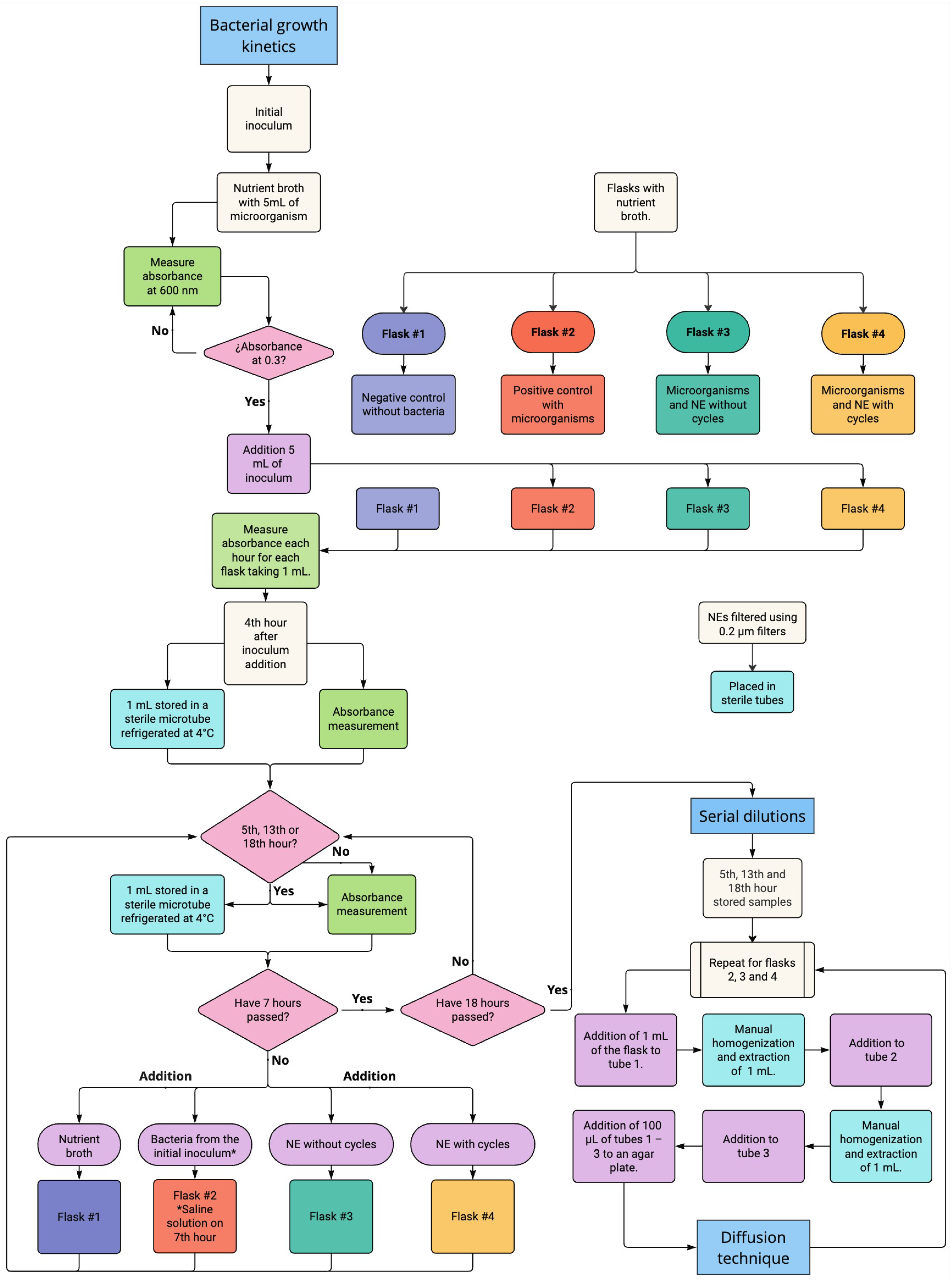
2.4. Bacterial Growth Kinetics and Serial Dilutions

2.4.1. Method of Optical Density Measurement During Growing

To determine the comparative efficacy of the NE before and after thermal cycles, a comparative kinematic growth test of bacteria was performed by measuring the relative absorbance using the OD concept [38,39]. The change in OD can be helpful for a qualitative determination of the efficacy of an NE compared to the kinetic growth of the microorganism without treatment. The kinetics were performed for more than an hour, and samples were taken at the 5th, 13th, and 18th hours of the experiment. Furthermore, serial dilutions were performed to approximate Colony-Forming Units (CFUs) using the SP technique, thus quantitatively determining the number of bacteria per millilitre of sample when exposed to NEs [40,41].

For the evaluation of the kinematic growth of the bacterial strains, the OD was measured using a Genesys 10S UV-Vis Spectrophotometer from Thermo Fisher Scientific (Waltham, MA, USA). The different bacterial strains were placed in 50 mL of nutrient broth. All bacterial strains used were placed under constant shaking at 80 rpm and 37 °C using the benchtop Shaking Incubator 222DS equipment, Labnet International, Inc. (Cary, NC, USA). Samples of 1 mL of these bacteria were taken at different times to apply the SP method and determine how many bacteria were still growing before and after the addition of NE. Each threefold sample was diluted in 9 mL of saline solution tubes at a concentration of 0.8% prepared using sodium chloride and distilled water to determine CFUs. From each dilution, 100 µL was taken and placed on the nutrient agar plate to then apply the SP diffusion technique.

The bacterial growth of the four bacterial strains was performed to evaluate the antibacterial efficacy of the NEs. The experiment was carried out over 18 h, measuring the OD of the samples each hour as a parameter of bacterial growth. The inoculum of each of the four bacteria (E. coli, S. aureus, B. subtilis, Salmonella spp.) was made in 50 mL of nutritive broth flasks by adding 5 mL of microorganisms to each. The inoculum was used until the OD reached a value of 0.3, considering the nutrient broth without bacteria as a blank.

During the inoculation stage, for each microorganism, four 50 mL flasks of nutrient broth were used for the different tests performed. The first flask consisted of the negative control, containing only nutrient broth to monitor any possible contamination during the experiment; no more was added to this flask during the experiment. For the rest of the flasks, 5 mL of inoculum, with an OD of 0.3 measured at 600 nm, was added at the beginning of the experiment. All flasks were placed in the incubator at 37 °C and 80 rpm during the 18 h of the experiment, measuring the OD of the samples each hour. At the fifth, sixth, seventh, thirteenth and eighteenth hours, 1 mL was taken for storage, and 1 mL was used for the measurement of OD from each sample.

In the fifth and sixth hours, in the positive control flask, 2 mL of inoculum was added after the 2 mL extraction to maintain the flask at 50 mL. In the seventh hour, 2 mL of sterile NaCl solution at 0.8% was added to this sample, thus compensating for the optical transparency of the NEs instead of adding the inoculum. In the third and fourth flasks, 2 mL of NE was added from the fifth to the seventh hour, applying an NE without thermal cycles to the third flask and with thermal cycles to the fourth. After the seventh hour, nothing else was added, and the microorganisms were allowed to grow under incubator conditions, taking OD measurements each hour and storage samples only at the 13th and 18th hours.

2.4.2. Method of Spread Plate in Serial Dilutions

Using 1 mL of storage samples for each hour, dilutions were performed in 9 mL saline solution tubes to determine the CFUs through serial dilutions and the nutritive agar SP diffusion technique. Three dilutions were conducted by taking 1 mL of the direct sample and adding it to 9 mL of saline solution in dilution 1 (1:10), then taking 1 mL of dilution 1 to 9 mL of dilution 2 (1:100), and finally taking 1 mL of dilution 2 and adding it to 9 mL of tube dilution 3 (1:1000). From each tube (dilutions 1, 2, and 3), 100 μL was placed on nutritive agar plates, applying the SP technique to nutrient broth agar plates. This procedure was performed to determine the number of colonies present in each sample and to approximate the living microorganisms taken at specific moments of the experiment.

This method allowed us to determine the number of colonies as shown in (1) by averaging the observed bacteria, considering the proportion of the dilution and the number of colonies present on the plate as follows:

$$\begin{array}{c}\hfill CFU={\displaystyle \frac{1}{n}}\sum _{i=1}^n{C}_i\times {10}^i\end{array}$$

(1)

where i the consecutive number of each dilution, n the total number of dilutions performed, and $C_i$ the number of colonies in each dilution.

3. Effect of Temperature on Physical Properties

In this section, the results for the physical changes in Palmarosa NE are presented, particularly those outcomes concerning the thermoresponsive behaviour of the droplet size distribution during heating–cooling cycles. According to Figure 1, DLS was used as the primary technique to determine the changes in droplet size over time. It was possible to observe transitional states of the stabilisation of the NE at different temperatures.

Table 1. Initial characterisation obtained for the one-year-old Palmarosa NE.

EO	Time	Max. (nm)	$\mathit{\mu }$ (nm)	$\mathit{\sigma }$ (nm)	PDI	Range	$\mathit{\zeta }$ (mV)
Palmarosa	1 year	8.82	9.94	3.00	0.30	15.717	−1.11

reports some initial characterisation values for our one-year-old NE [28], prior to the subsequent thermoresponsivity tests. As in our previous report, the range corresponds to the main width region containing $99\%$ of the droplets.

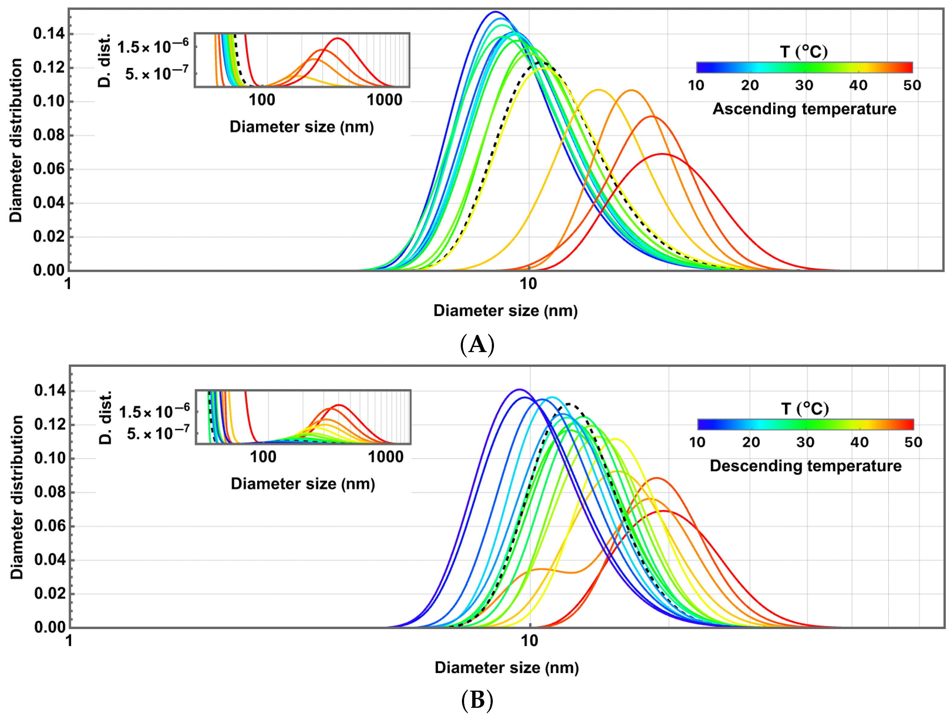
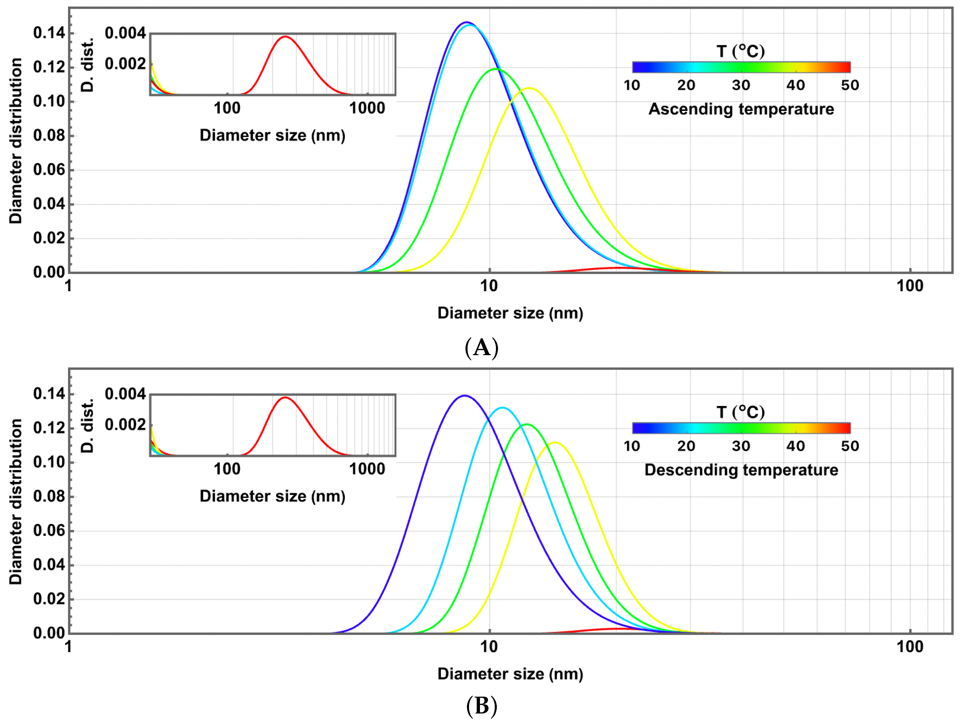
3.1. Initial Thermoresponsive Droplet Size Analysis

Stability is a crucial property that is expected in emulsions. Moreover, the most current agreement on the classification of microemulsions (MEs) and NEs regards not only their droplet size characteristics but also their type of stability, thermodynamic or kinetic [17,35,42], respectively. In NEs, this property indicates whether the system will remain characterised by a droplet-size nanoscale for an extended period or whether it will transition into a conventional emulsion, thereby losing the properties potentiated by this scale. This situation is relevant if the NE requires long storage periods before its final application. Previous DLS-based droplet size analysis showed that Palmarosa NE with 5% essential oil had a very stable average size. With an initial characteristic diameter of 11.4 nm and a PDI of 0.226, these values evolved one year later to 9.94 nm and 0.300 while the NE was kept at a reasonably constant room temperature and stored in darkness.

3.2. Thermoresponsivity and Fast Changes in Temperature

To track the behaviour of the NE droplet size at different temperatures, it was initially stabilised at a temperature of 10 °C. Subsequently, heating cycles were established up to a limit of 50 °C, returning to the initial temperature, thus setting a heating–cooling cycle. The DLS equipment was programmed to heat the sample, reach a target temperature, and then perform measurements of the droplet size distribution (after a waiting time for stabilisation). In this process, the measurement for the distribution mode by the number of droplets was selected. However, structural changes in the droplet size of NEs are not instantaneous processes. Once an average temperature established by the DLS instrument has been reached, the coalescence and flocculation processes continue, because we are working with a non-homogeneous system. For this reason, three methodologies were established to precisely observe this process.

In the first methodology, the DLS equipment reached a detailed series of temperatures 10, 12.5, 15, …, 50 °C spaced out every 2.5 °C and then waited two minutes for stabilisation before making the distribution measurement, while maintaining each temperature fixed. At the end of the measurement, the machine heated the sample again to the next temperature and waited again for two minutes before taking the next measurement. This procedure continued by increasing the temperature until the temperature of 50 °C was reached, letting two minutes pass, and measuring again before starting the cooling cycle. Then, it continued to decrease the temperature by 2.5 °C at each step, again requiring a waiting period of two minutes. The entire cycle ended with the sample cooled to 10 °C, waiting two minutes for each measurement, and taking the last measurement.

Although DLS equipment typically increases or decreases the temperature at a rate of approximately 2.5 °C per minute, the waiting period at a constant temperature was introduced prior to each measurement in all methodological cases. This waiting time enabled the observation of a detected underlying recovery phenomenon. Three identical independent repetitions of this experiment were performed; then the distribution data were averaged to reduce any variability due to other fluctuation factors. This average is reported at each temperature in the following analysis.

Figure 2 shows the corresponding heating and cooling cycles, indicating the temperatures in colour in agreement with the included colour scale in the upper right. The horizontal axis shows the diameters of the droplet distribution on a logarithmic scale, whereas the vertical axis indicates the value of the normalised distribution for each diameter. The upper inset reveals a small bimodal distribution appearing between 100 and 1000 nm. It should be noted how extensive this distribution is by virtue of the logarithmic scale, despite its much lower height on the vertical axis.

The different phenomena that occurred are remarkable. First, as expected during the heating cycle (Figure 2A), at higher temperatures, the coalescence of the droplets increases, moving the maximum of the distribution to the right, towards a greater number of droplets of larger diameter. However, this phenomenon is not necessarily linear, occasionally exhibiting some setbacks at that maximum. The process appears to be accelerated around 40 °C, making the secondary peak of the distribution much more noticeable, as illustrated in the inset. For the cooling cycle (Figure 2B), a much slower and more gradual re-establishment is observed. In both cases, the body temperature of 37.5 °C is highlighted with a black dotted line. Note that for a temperature of 45 °C, a trimodal distribution appears, preserving the far distribution between 100 and 1000 nm. Note also a slight shift to the right of the distribution at 10 °C during the cooling cycle relative to the initial one during the heating cycle.

Because nanoemulsions typically exhibit kinetic rather than thermodynamic stability, temperature changes can induce irreversible alterations such as flocculation and coalescence. The hysteresis analysis indicated that, in general, no strictly irreversible phenomena occurred since the heating and cooling cycles did not follow identical paths. Nonetheless, a delayed recovery process was observed in which the nanoemulsion gradually returned to its original droplet size distribution. This behaviour is of particular industrial relevance to maintain the stability of the product.

3.3. Dynamical Thermoresponsivity Under Maintained Changes in Temperature

From the previous analysis, we inferred that each heating and cooling process within the NE, even achieving a stable temperature, involved a series of internal processes that were not immediate in the distribution of droplets associated with coalescence. Therefore, in our analysis, we devised a couple of additional methodologies to analyse the thermoresponsive process in a more comprehensive way. For the second and third approximations, the heating and cooling cycle was repeated at intervals of 10 °C, that is, $10,20,\dots ,50 °\mathrm{C}$ for heating and cooling. However, in these cases, the waiting period for the measurement at fixed temperature was extended to five and twenty minutes, respectively. Each of these approaches sought to better approximate the equilibrium states with constant temperature but still within broader heating and cooling cycles. Similarly to Figure 2 previously described and presented, Figure 3 and Figure 4 present the results of these complementary analyses. In each case, as before, two panels were prepared, one for heating and one for cooling.

Thus, Figure 3A shows the distributions obtained with 5 min of waiting at the temperatures depicted in colour, as before. The dynamic process is observed to be more uniform as the temperature increases, but it accelerates at higher temperatures. Notice how the secondary peak is now visible on the scale presented in the inset only for 50 °C, despite existing at lower temperatures (secondary peaks at other temperatures still exist, but on a much smaller and negligible scale). This behaviour shows a closer approximation to a state of equilibrium after 5 min at a stable temperature. Figure 3B shows a similar and more uniform behaviour when returning, with a configuration very similar to the initial one at 10 °C. Although the position of the maximum in the distribution is now much more similar to that observed in Figure 2A,B, it is possible to see a decrease in its height, suggesting that the secondary peak prevails in the final stage (although negligible in the upper inset of Figure 3B). The behaviour of the NE at 50 °C stands out, where the original distribution has practically disappeared, while the substitute distribution between 100 and 1000 nm dominates.

Finally, for the case with waiting times of 20 min, we observe some additional aspects in Figure 4A,B, for the heating and cooling stages, respectively. During warming (Figure 4A), for temperatures of $10,20,$ and $30 °\mathrm{C}$, we observe similar distributions, showing that in this range the NE had the ability to adapt to the increase in temperature while remaining stable. However, a thermodynamic change is seen in the distribution with droplets larger than around 100 nm (not appreciable in the inset at the scale shown). For temperatures of 40 and 50 °C, the original distribution gives rise to trimodal distributions with droplets smaller than the initial characteristic diameter of 10 nm and at extinction, generating an additional distribution that shifts to the zone of 100 nm (see inset) and a lower tertiary distribution between 100 and 1000 nm. This process, closer to thermal equilibrium at each fixed temperature, illustrates how some smaller droplets are highly stable and practically resistant to temperature changes below 40 °C. As the temperature increases, larger droplets begin to agglomerate and coalesce, which can give rise to distributions with different characteristic diameters. During cooling (Figure 4B), the system returns more slowly and evenly almost to its initial configuration, but with a small increase in its characteristic diameter of nearly 2 nm.

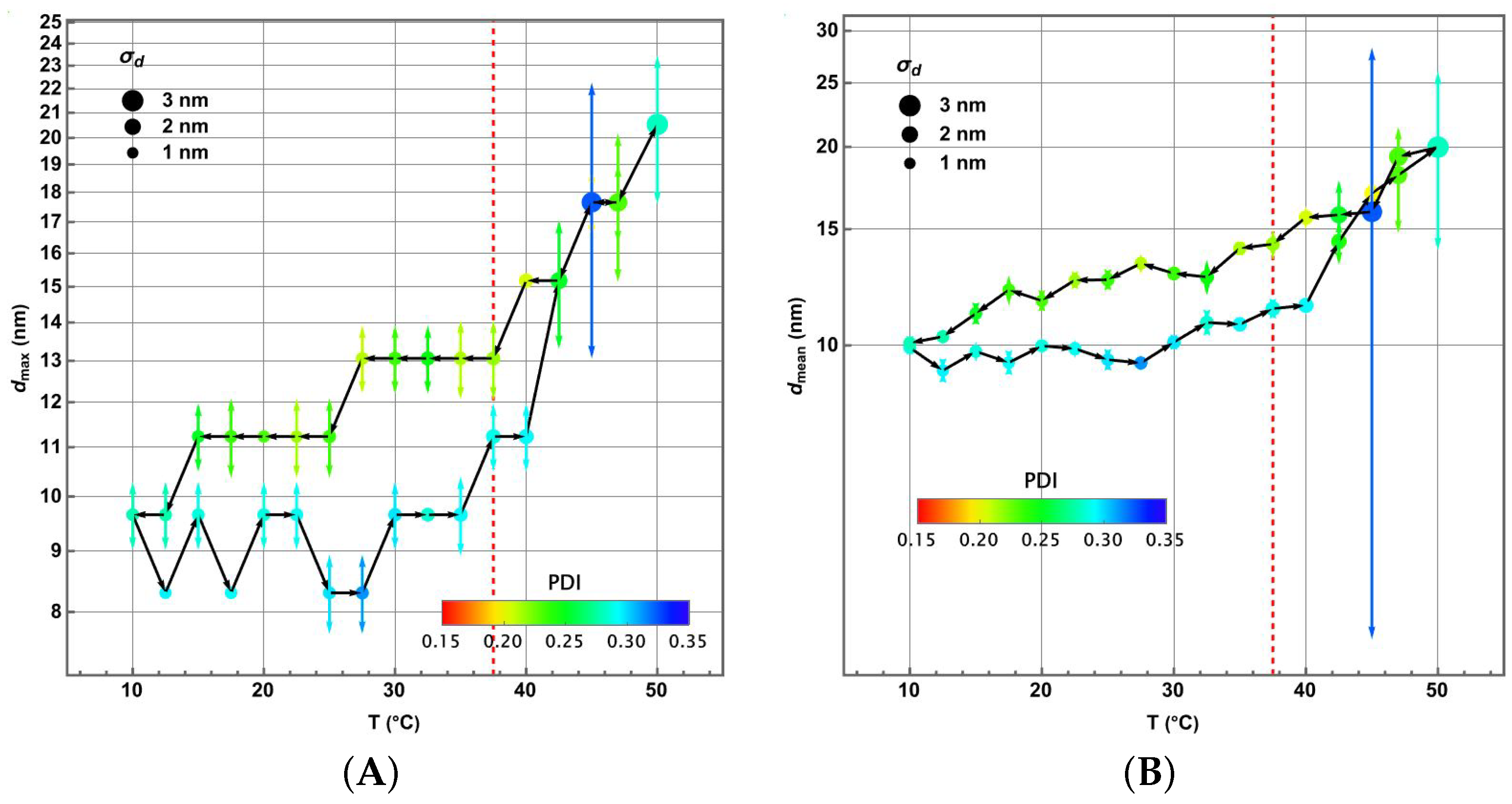
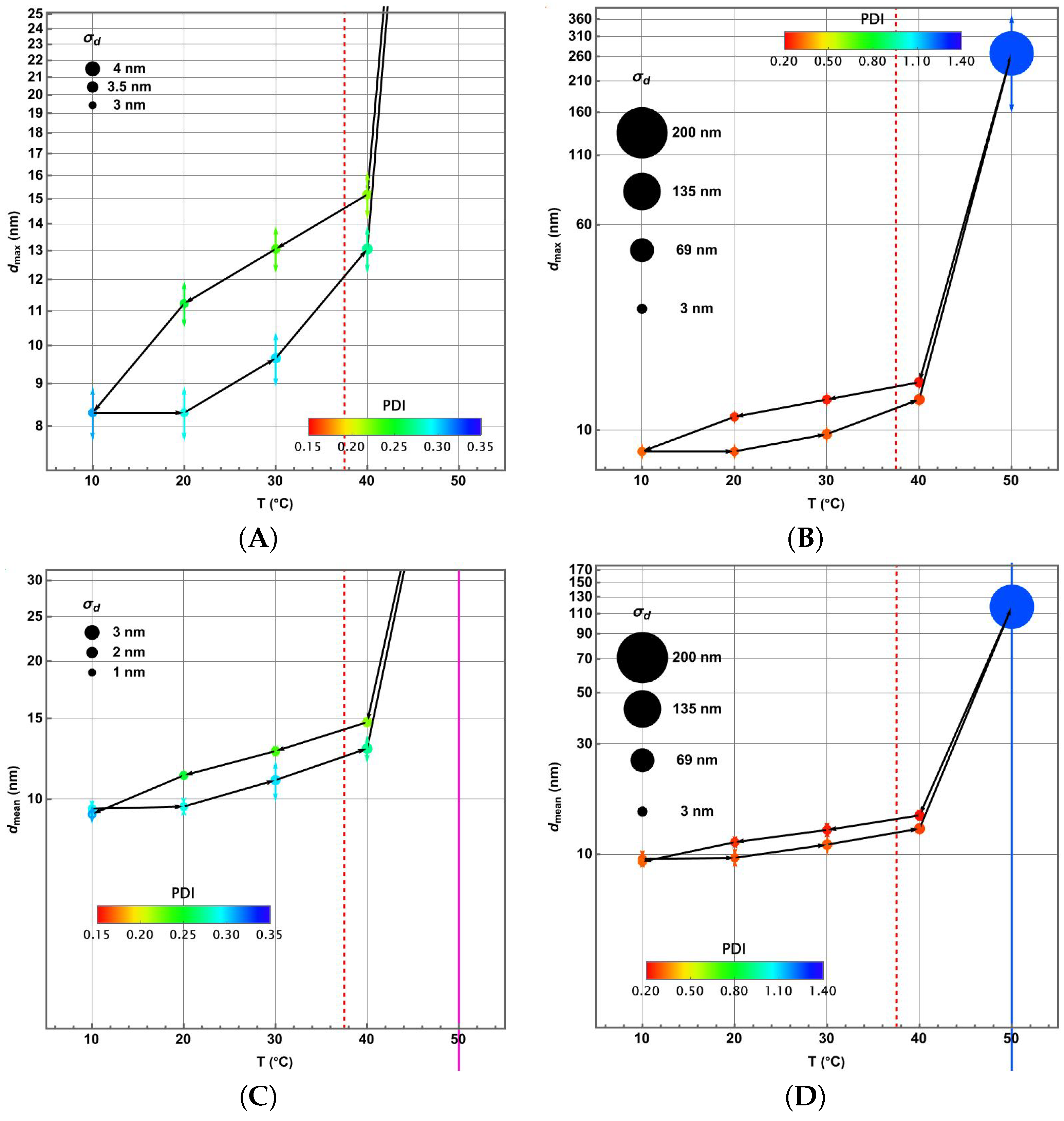
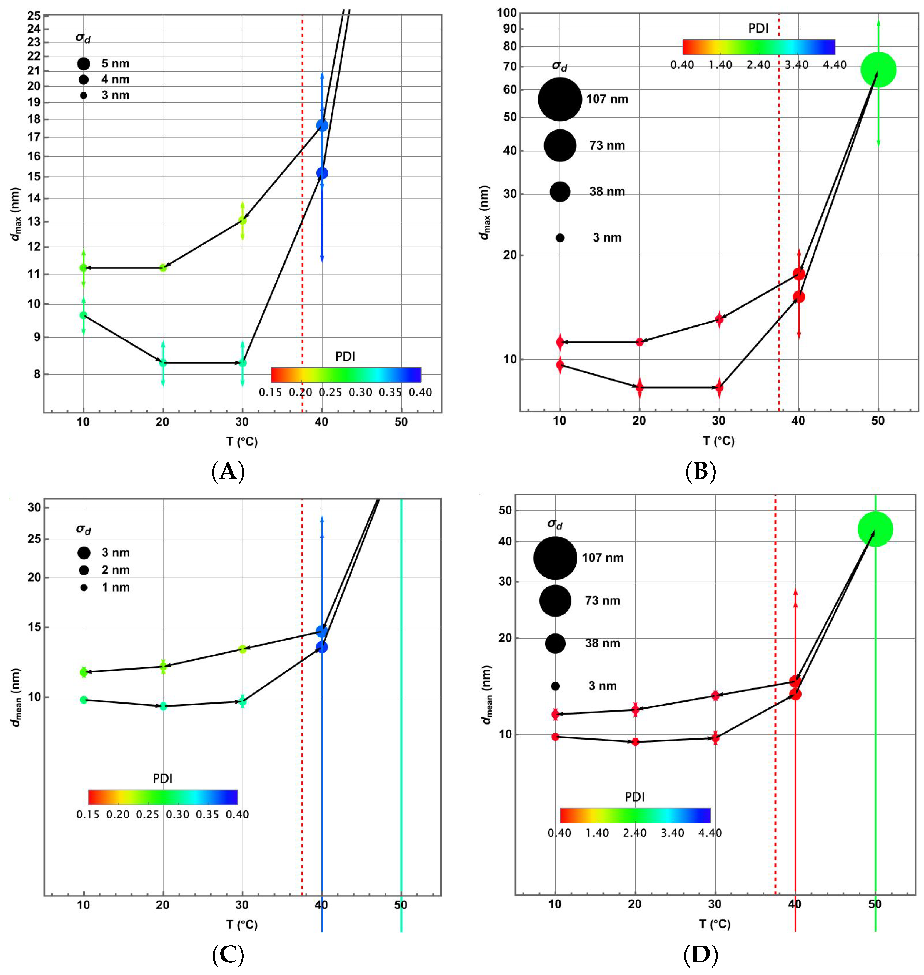
3.4. Piecewise Hysteresis Diagrams for Droplet Sizes

In this section, we analyse the thermoresponsive effects during the previous heating–cooling cycles from a general perspective by examining the behaviour of the characteristic diameter and the mean diameter of the distribution at each temperature and waiting time to obtain the distribution measurement. The errors reported in the characteristic and mean diameters refer to one standard deviation obtained by performing each three- fold experiment.

For the 2 min waiting time before measurement, the evolution data during the heating and cooling cycle are represented in Figure 5A,B for the characteristic diameter (in nm), $d_{max}$ (peak of distribution), and the mean radius, $d_{mean}$, respectively, as a function of temperature, T (horizontal axis, in °C). Both graphs report the margin of error obtained from the triplicate repetition of the experiment as vertical error bars. Additionally, the PDI is reported in colour, according to the bar included as an inset. The size of the reported point refers to the standard deviation of the average distribution (of the three experiments) at each temperature, according to the scale included in the form of black circles.

In Figure 5A, a non-linear evolution is evident with setbacks in the characteristic diameter $d_{max}$. These setbacks seem real because they are still observed within the margin of error obtained. As noted in the analysis of the previous section, only temperatures above 37.5 °C seem to show a clear coalescence dynamic within the NE. Notable errors are observed for temperatures closer to 50 °C, where repeatability is not faithfully reached in the three experiments. Despite this, the cooling period again shows a very stable behaviour that exactly closes the cycle with great consistency. The red dotted line marks the body temperature of 37.5 °C, which is useful to discuss the topical use of NE. Except for the highest temperatures, the standard deviation of the distribution is reasonably stable. The increase in PDI and the errors in $d_{max}$ on average around 45 °C are particularly notable. A similar but much smoother behaviour is observed for the average diameter $d_{mean}$ (Figure 5B), but with smaller setbacks that nevertheless, in this case, remain within the experimental error zone. Note how in both characterisation parameters, there is unpredictable behaviour at temperatures close to 50 °C. Despite the hysteresis cycle whereby the heating and cooling periods do not undergo the same behaviour, there is an imperceptible change for both representative diameters at the end of the cycle at 10 °C. We can also note that distributions at low temperatures show a right chirality observed at room temperature in [28], generating $d_{max}<d_{mean}$. However, this behaviour seems to be lost for higher temperatures (although the level of error at these temperatures does not allow us to conclusively assert it).

For the heating–cooling cycle with 5 min of waiting before the droplet size dispersion measurement, Figure 6 presents the corresponding results of Figure 3. In this case, the characteristic diameter is reported for convenience in Figure 6A,B, showing, respectively, a partial view at low temperatures and the global view afterwards. Similarly, Figure 6C,D show the mean diameters in a similar way. Note that each panel includes a different scale to report the PDI. Although fewer temperatures are reported, we observe a smoothing in the process, primarily because of the extended waiting time. Notice how, for $d_{mean}$, the process becomes similar to that of $d_{max}$. The variation in PDI is stable and reduced with respect to the previous case. The average diameter at the end of the process has increased slightly from its initial value. Again, a large dispersion is observed for the temperature of 50 °C, as well as a remarkable variability in the experiments that leads to higher errors, mainly due to the multimodality of the distribution reported by the DLS equipment. The stable behaviour above body temperature ($40>37.5 °\mathrm{C}$) is appreciable.

Like the previous figure, Figure 7 shows the case for 20 min of waiting. Figure 7B,D show the same plots, but with a larger vertical representation of the scale. Some differences are notable, for example, a reduction and increase in the characteristic diameter $d_{max}$ due to the longer stabilisation time (Figure 7A,B). This behaviour is not observable in the mean diameter $d_{mean}$, which shows a smoother behaviour now than in the previous cases (Figure 7C,D).

Finally, a hysteresis process appears clearer, with a slight increase in both parameters. Again, although the NE shows remarkable stability behaviour when returning to low temperatures, a more complex process prevails at the highest temperature studied (50 °C) but even more consistent in experimental repetitions than in the case with waiting times of 5 min. For a complementary analysis, the detailed source data for Figure 5, Figure 6 and Figure 7 can be consulted in

Table A1. Summarised NE parameters (maximum or characteristic diameter, mean diameter, distribution standard deviation, and PDI) present through each thermoresponsivity test, at 2, 5, and 20 min of waiting before performing the droplet size distribution measurement. The errors reported for the diameters correspond to those arising from the three-fold test for each waiting time.

Measure	Time (min)	Ascending Temperature T (°C)					Descending Temperature T (°C)
		10	20	30	40	50	40	30	20	10
Max. (nm)	2	9.65 ± 0.64	9.65 ± 0.64	9.65 ± 0.64	11.20 ± 0.74	20.50 ± 2.93	15.20 ± 0.00	13.10 ± 0.86	11.20 ± 0.00	9.65 ± 0.64
	5	8.30 ± 0.64	8.30 ± 0.64	9.65 ± 0.74	13.10 ± 0.86	267.00 ± 109.00	15.20 ± 1.00	13.10 ± 0.86	11.20 ± 0.74	8.30 ± 0.64
	20	9.65 ± 0.64	8.30 ± 0.64	8.30 ± 0.64	15.20 ± 3.79	68.70 ± 27.90	17.70 ± 3.35	13.10 ± 0.86	11.20 ± 0.00	11.20 ± 0.74
$\mu$ (nm)	2	9.92 ± 0.22	9.99 ± 0.28	10.10 ± 0.19	11.50 ± 0.37	20.00 ± 6.05	15.60 ± 0.62	12.90 ± 0.43	11.70 ± 0.10	10.10 ± 0.21
	5	9.53 ± 0.04	9.64 ± 0.01	11.00 ± 1.17	12.90 ± 0.96	118.00 ± 16,500.00	14.70 ± 0.45	12.70 ± 0.23	11.30 ± 0.35	9.27 ± 0.48
	20	9.85 ± 0.30	9.48 ± 0.32	9.76 ± 0.03	13.40 ± 13.00	43.80 ± 1730.00	14.60 ± 14.20	13.20 ± 0.24	11.90 ± 0.02	11.60 ± 0.13
$\sigma$ (nm)	2	2.84	2.87	3.01	3.38	5.62	3.21	3.02	2.71	2.81
	5	2.78	2.78	3.29	3.52	148.00	3.23	2.97	2.87	2.87
	20	2.89	2.90	2.98	5.02	107.00	5.33	3.07	2.88	2.93
PDI	2	0.29	0.29	0.30	0.29	0.28	0.21	0.23	0.23	0.28
	5	0.29	0.29	0.30	0.27	1.26	0.22	0.23	0.25	0.31
	20	0.29	0.31	0.31	0.38	2.45	0.36	0.23	0.24	0.25

.

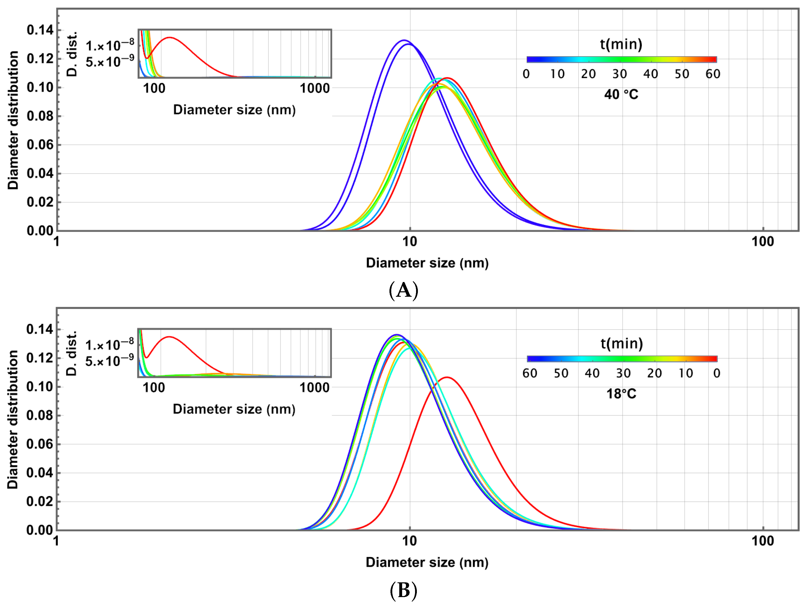
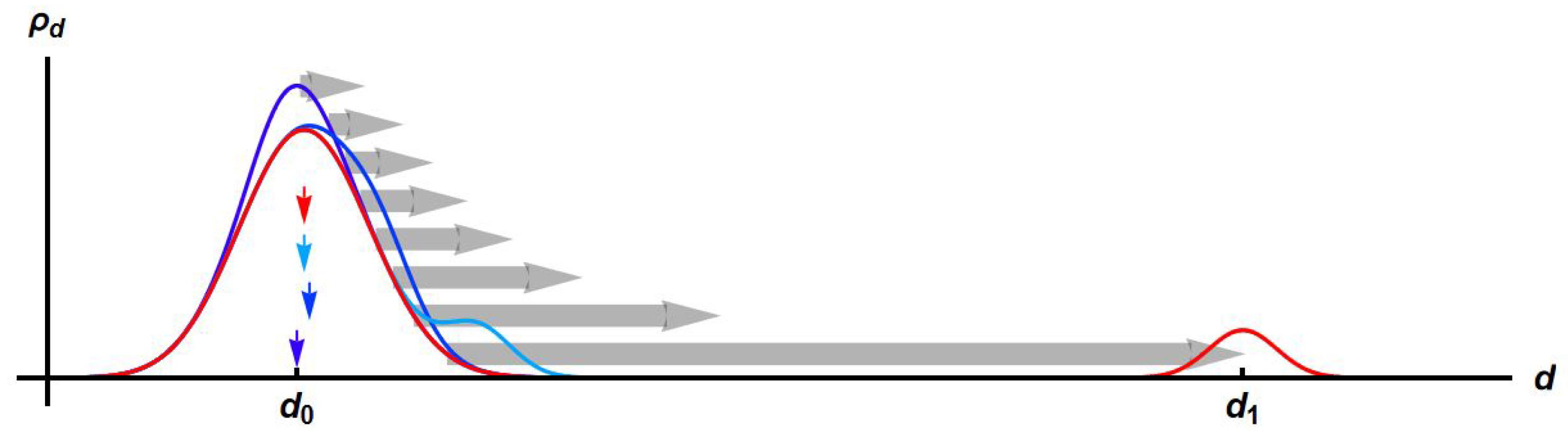
3.5. Dynamical Process Observed on Droplet Sizes Under a Maintained Raising or Lowering of Temperature

In previous analyses, it was observed that NE had high stability in the face of temperature changes, particularly for moderate temperature changes below 40 °C. However, the NE underwent a gradual fluctuation process in which the larger diameter particles seemed to change faster with a more noticeable coalescence process. This non-uniform change in all droplets generated an appreciable change in droplet size distribution. However, we previously followed a gradual heating and cooling process despite measurement pauses at constant temperature before continuing the permanent thermodynamic process to form a complete cycle. The most widespread heating pauses suggested reaching an apparent state of equilibrium that gave rise to metastable distributions that, however, changed again with a new change in temperature.

In the next test, we extended the stabilisation period until we reached an appreciable equilibrium in the distribution with the goal of achieving three final temperatures, 30 °C, 40 °C, and 50 °C, in a single step departing from laboratory temperature (18 °C). It reproduced a more typical heating and cooling process for a commercial nanoemulsion. Finally, the cooling cycle was repeated at the starting temperature. In that case, several measurements of the droplet size distribution were taken every 2.5 min, although for the sake of clarity during the comparison, only those separated by periods of 10 min are reported. In each case, the experiment was performed three times to take the average distribution at each time. Figure 8, Figure 9 and Figure 10 present these results.

Figure 8A shows the rapid heating from 18 to 30 °C by the DLS equipment in the first minute and the maintenance of the latter temperature until an observable equilibrium in the droplet size distribution is reached. Thus, the initial distribution at 18 °C is shown and one minute after the first measurement at 30 °C, followed by measurements made at minutes 11, 21, …, 61 min. Each measurement time is illustrated with a different colour according to the included scale. The fast fluctuation from 18 °C to 30 °C shows a sharp change in the characteristic diameter (first two graphs in blue, with peaks at about 8.82 and 11.78 nm). Even so, in that case, the NE exhibits great stability and notably an oscillation in the characteristic diameter after it reaches slightly higher values, maintaining a final characteristic diameter of approximately 10.33 nm (red, minute 61), greater than the initial diameter of 8.82 nm (blue, minute 0). This final distribution is achieved at the cost of the appearance of a bimodal distribution with a maximum close to 1000 nm (see the inset). This second maximum ends up being much lower than the first but leaving evidence of it, while the primary peak returns to a slightly lower value after its intermediate maximum increase. It should be noted that this secondary peak moves towards much larger diameters until it stabilises, but its apparently much smaller size is due to the logarithmic scale used. Once equilibrium is reached (red, minute 61), the sample is cooled by the DLS equipment in one minute to 18 °C again (see Figure 8B). In this case, the fluctuations in the distribution turn out to be much more uniform, although a sudden reduction is also observed first, exhibiting oscillations until reaching the final distribution (blue, minute 61) with a characteristic diameter at the beginning of the experiment, 10.22 nm, similar to that at the end of the cycle at 30 °C.

Subsequently, the NE was heated to 40 °C following the methodology described above. In that case, the DLS instrument reached this temperature again in the first minute and the spectrum barely underwent a minimal displacement, increasing the droplet size over the initial 8.82 nm, as can be seen in Figure 9A. However, 10 min later, the distribution had moved noticeably and remained almost unchanged until its stabilisation 60 min later, reaching a characteristic diameter of 17.12 nm (red, minute 61). A bimodal distribution was achieved with a secondary peak above 100 nm (see inset). When the equipment cooled the sample back to 18 °C (see Figure 9B), this process occurred again within one minute, and the NE rapidly returned almost to its original position and stabilised almost again 60 min after cooling with a characteristic diameter of 9.14 nm (blue, minute 61). At that stage, no secondary distribution was practically appreciable compared to the scale of the one that appeared at the end of the warming cycle (see inset).

The last cycle considered was 50 °C following the previous steps. Figure 10A shows the process of going from 18 °C to 50 °C in the first minute (first two graphs in blue) with a rapid increase in characteristic diameter from 8.82 to 16.27 nm (red, minute 61). The distribution maintained at a constant temperature of 50 °C fluctuates until it stabilises after 60 min in an approximately bimodal distribution (see the inset) with a primary peak at 17.12 nm. Note the deformation of the distribution around 40 min due to coalescence dynamics. The secondary peak shows a gradual dynamic until it stabilises around 300–400 nm as part of a very wide distribution. Figure 10B shows the cooling of the sample from 50 °C to 18 °C in the first minute, again resulting in a sudden reduction in the characteristic diameter to 11.78 nm and then a stabilisation showing nearby oscillations until the characteristic diameter is located at 11.20 nm (red, minute 61). There, a wide secondary distribution prevails around 300–400 nm.

3.6. Some Remarks About Polydispersity Through the Heating and Cooling Cycles

Some considerations for polydispersity should still be discussed. Although this is a composite measure in terms defined for this study, $\mathrm{PDI}={\displaystyle \frac{\sigma }{\mu }}$, this quantity still helps to identify the trajectories in the hysteresis cycle. As can be seen in Figure 5A,B, Figure 6A,C and Figure 7A,C, there is a clear differentiation between the heating cycle and the cooling cycle in terms of PDI, which is notably higher for the former. This quantitatively illustrates the behaviour previously observed; in the heating phase, the droplet size average increases more slowly than do the respective dispersions, generating an increase in the PDI. This aspect becomes relevant for commercial applications because the droplet size distribution at the nanoscale could be efficiently recovered by cooling NEs. Instead, during cooling, despite the fact that the NE goes through similar standard deviations, the average droplet size decreases more rapidly than during heating, resulting in lower PDIs than in the initial cycle. This behaviour characterises both periods of the thermal cycle, although there is almost perfect agreement between its beginning and end. However, for temperatures between 40 °C and 50 °C (see Figure 6B,D and Figure 7B,D, being aware of the change in scale for the PDI), there is erratic behaviour in this phenomenon, with notorious variations in the results of the experimental repetitions, which, as already mentioned, can have multiple explanations, from greater disorder in the system to a lack of precision in obtaining the distributions by the DLS method.

3.7. Statistical Analysis of Meaningful Differences in Physical Parameters Characterising Droplet Size Distributions

Datasets for Figure 5, Figure 6 and Figure 7 are reported in Table A1 in Appendix A. We can compare each of the physical parameters $\mathrm{Max}.,\mu ,\sigma$ and PDI characterising droplet size distributions under two different treatments, waiting times (2, 5, 20 min) and temperature (10, 20, …, 40, 50, 40, …, 10 °C). In fact, using a two-factor ANOVA test, together with Tukey’s method for pairwise comparisons as a post-test [43], we found meaningful statistical differences through each different treatment. See the details in Appendix E.

Using a significance level of $\alpha =0.01$, the two-factor ANOVA test did not find significant statistical differences among treatments for any physical parameter, with the exception of $\sigma$ as a function of temperature (p-value became $p=0.009<\alpha$), thus denoting a sensible change in droplet size dispersion during heating–cooling cycles. Consistently, the Tukey post-test only detected some meaningful differences for some temperatures, not for waiting times. This is interesting because the observed changes were not sufficiently meaningful in statistical terms, highlighting the stability of the NE under thermoresponsive factors.

In the Tukey post-test (see Appendix E, the first group of differences appeared for $\mu$ (there were no significant differences for the characteristic diameter $\mathrm{Max}.$) at 50 °C compared to 10, 20, and 30 °C during the heating cycle, as well as between 50 °C and the final temperature 10 °C at the end of the cooling cycle. This clearly shows the different behaviour for the highest temperature, 50 °C. For $\sigma$, the detected paired differences corresponded to the highest temperature 50 °C and each of the other temperatures in the heating–cooling cycle, just confirming the previous finding of the ANOVA test. Significant differences for PDI appeared between that for 50 °C and all other cooling temperatures, highlighting the rapid recovery of the droplet size distribution by cooling.

3.8. Discussion: Droplet Size Thermoresponsivity

The first part of our study analysed the thermoresponsive behaviour of an NE that had shown high stability for one year at room temperature [28]. There, controlled changes and, in particular, the heating and cooling cycles showed some of its physical properties. Thus, in the face of relatively rapid gradual temperature changes (Figure 2), a moderate shift in the droplet size distribution was observed, which was primarily reversible but still with a small irreversible hysteresis effect. A closer quasi-static analysis showed that the NE still remained in a state of enduring thermodynamic disequilibrium, despite reaching an average temperature reported by the DLS equipment during the heating or cooling process (Figure 3 and Figure 4). Once a critical temperature was exceeded (in our study around 40 °C), bimodal distributions arose, which nevertheless seemed to be re-established during the cooling cycle. Thus, the more the NE was allowed to stabilise, the more the quasi-stable distributions showed a recovery toward the original distribution, but only if this critical temperature was not exceeded. If this was exceeded, there were global changes in the distribution that nevertheless largely disappeared when it was cooled again.

However, the heating and cooling cycles exhibited hysteresis with a very close coincidence with the initial droplet size distribution (Figure 5, Figure 6 and Figure 7). The differential behaviour between the characteristic diameter, $d_{max}$, and the mean diameter, $d_{mean}$, showed that the above process affected droplets of different sizes differently. The quasi-static behaviour revealed a minimal hysteresis effect, where the distribution did not return to its original state, generating small groups of much larger droplets due to coalescence or flocculation processes. Given the almost exact return to the initial condition, it is possible that flocculation dominated the process, allowing the droplets to separate upon return to low temperatures, although some larger droplets were temporarily maintained.

The transition processes between only two temperatures showed this behaviour more clearly. Thermodynamic equilibrium was not reached when the DLS system estimated an average temperature in the sample but much later, when the distribution reached a metastable state. This process was highly resilient to moderate temperature changes.

A technical aspect cannot be overlooked. DLS equipment uses light-intensity scattering to estimate the particle size in the NE. This estimation assumes the sphericity of the droplets to interpret light-intensity scattering spectra, so the dynamics of the droplet size is certainly inappropriate [44]. The ongoing flocculation and coalescence processes can falsify the results in large droplet distributions, which these instruments interpret as individual droplets and not as flocs or groups of particles under melting [45]. Therefore, in general, tiny errors in measurements of the width of the distributions by backscattering on these machines should be taken with caution, since they can be amplified when transformed into number or volume distributions [46]. In addition, repeated measurements on DLS equipment often introduce certain variability depending on preparation; this was the reason why we performed tests in triplicate to better assess the result in the distribution [47].

In addition to the imprecision and care of the measurements made by DLS equipment, details must be added within the process outside the equilibrium where the timescales for droplet rupture do not refer to instantaneous processes, so measurements with longer waiting times generally provide better precision of the NE behaviour [48]. However, in comparison, high stability under heating in O/W NEs has been observed in other studies [49], particularly in analyses of programmed temperature ramps such as those carried out here [50]. There is also evidence that heat-destabilised NEs can be restored or rejuvenated by raising them to an ideal temperature for a certain period [51].

The results of this study show that the smaller droplets in the distributions are highly stable, while the larger ones are more susceptible to the processes of coalescence and flocculation, although they exhibit high reversibility. Figure 11 illustrates a schematic simulation of this process in which those areas of the distribution of the larger droplets move more rapidly to the right toward larger diameters. The grey arrows show how large droplets can coalesce more easily. This process is characterised by a gradual appearance of a bimodal (or multimodal, not illustrated) distribution that produces oscillatory behaviour in the characteristic droplet size (see corresponding vertical arrows indicating this characteristic diameter in the dynamics of the distribution) due to the redistribution of the number of droplets for each diameter.

4. Comparative Chemical Composition

As previously commented on and depicted in Figure 1, the composition of NEs and their respective raw materials was studied using FTIR coupled with ATR for their components and interactions. After the elaboration of the NE, it was initially characterised to determine its chemical composition. It involved EO, raw components such as water and Eumulgin, and the proper NE in its fabrication. A new final analysis was performed at the end of the thermoresponsive tests. Each sample used here was exposed at least 18 times to thermal cycles of heating and cooling between 10 and 50 °C during the previous thermoresponsive tests already presented. Thus, we evaluated any possible chemical composition changes in the NE after the heating and cooling cycles.

As a verification test, the composition analysis was tracked looking for the preservation of the main components in the NE, those particularly relevant for their antibacterial and antifungal characteristics. Thus, FTIR analyses were performed on the sample and its raw materials. Figure 12 shows the results in both stages. The plot includes the spectrum for the Palmarosa essential oil (red), Eumulgin surfactant (orange), initial NE upon fabrication (blue), and final NE after thermoresponsive tests (green) in agreement with the upper legend for a direct comparison between them.

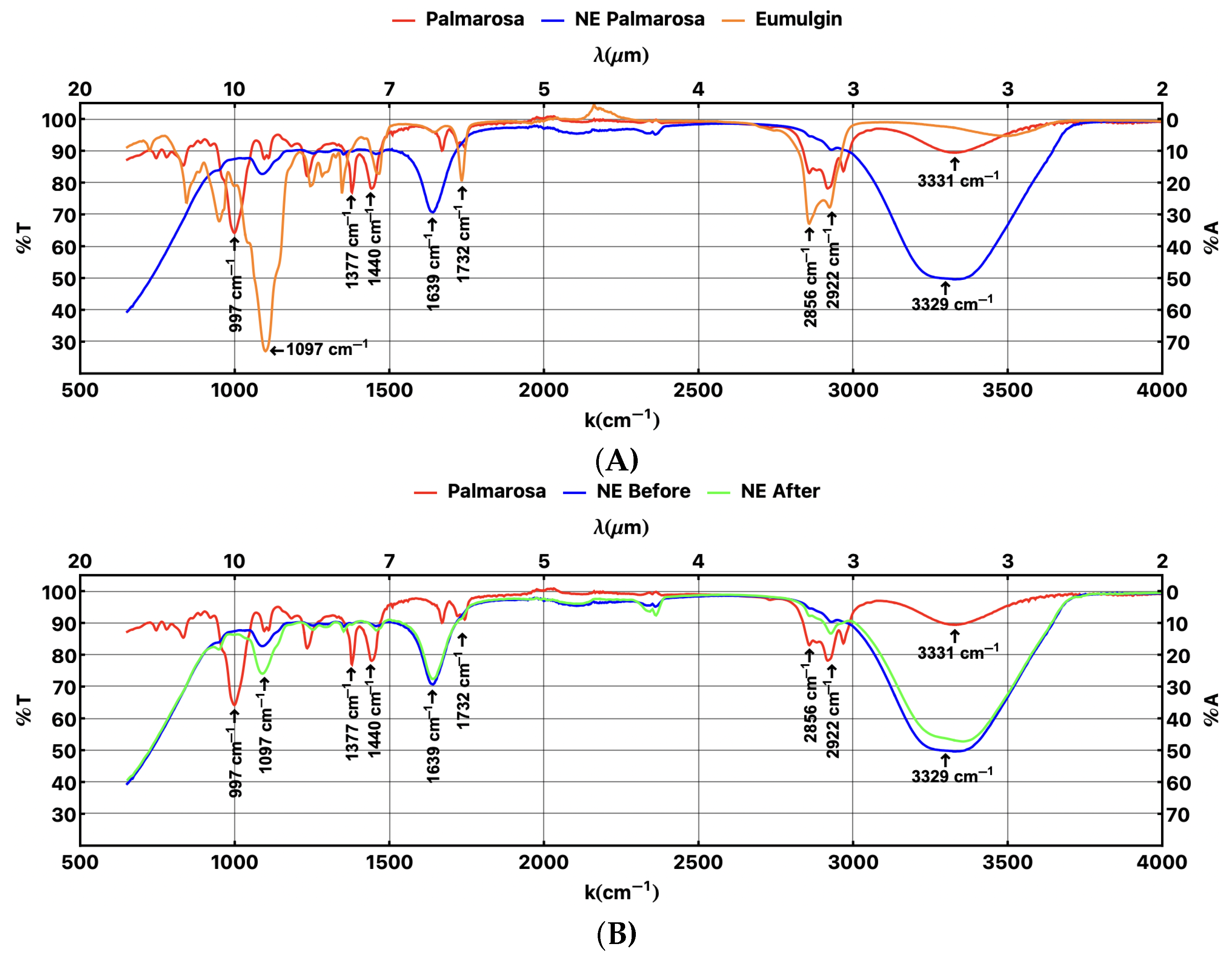
4.1. Initial Composition Analysis

In the plots, the lower and upper horizontal axes show the wavenumber (k) and the wavelength ($\lambda$), respectively, to facilitate the interpretation of the spectrum. The left vertical axis reports the transmittance (%T) and the right vertical, the absorption. Each plot indicates some relevant wavenumbers that reveal certain chemical groups in the NE composition. Analysing the raw materials observed in Figure 12A, the Eumulgin spectrum (orange) was included, showing a band at 2922 ${\mathrm{cm}}^{-1}$ corresponding to the stretching of O-H of the carboxylic acid. Also, around 1732 ${\mathrm{cm}}^{-1}$, a stretching C=O vibration is produced in the acid group. At 1097 ${\mathrm{cm}}^{-1}$, a noticeable band corresponds to the C-O stretching that coincides with the carboxylic acid of Eumulgin. Two characteristic bands at 1639 ${\mathrm{cm}}^{-1}$ and 3329 ${\mathrm{cm}}^{-1}$ correspond to the water spectrum, widely reported in the literature [28].

However, the obtained Palmarosa EO spectrum is in agreement with other studies, such as those published by FAO and [52], which analysed the main compound of Palmarosa, geraniol. One of the main bands observed in this spectrum can be found at 3331 ${\mathrm{cm}}^{-1}$, corresponding to the stretching of the O-H of the alcoholic group present in the molecule. Alkane and alkene vibrations can be found in the range of 3000–2800 ${\mathrm{cm}}^{-1}$. In particular, a stretching of 1639 ${\mathrm{cm}}^{-1}$ C=C is observed. Another relevant band found in the spectrum has a wavenumber of 997 ${\mathrm{cm}}^{-1}$, associated with the C-O stretching of the alcohol group.

It can be observed that the NE spectrum differs from that of both EO and Eumulgin as a result of the overall composition. Because the continuous phase has a higher proportion than the rest of the components, it resembles the distilled water spectrum with some slight differences. The main broadband observed around 3129 ${\mathrm{cm}}^{-1}$ is associated with the O-H bond present in both EO and distilled water. At 1639 ${\mathrm{cm}}^{-1}$, there is the C=O stretching that can be found at similar wavenumbers, both in the surfactant and the Palmarosa EO. The band mostly corresponds to the continuous phase; however, interactions between components may have caused a shift in the observed bands of the NE. Another band can be seen at 1097 ${\mathrm{cm}}^{-1}$, which corresponds to the surfactant and increases in absorption as a higher concentration of surfactant is added, a phenomenon seen in [52].

4.2. Effect of Thermal Cycles on Composition of NEs

Figure 12B shows the changes in the composition of the NE before and after thermal cycles. This was useful to determine to what degree the composition changed after several thermal cycles. One of the main differences between both spectra can be seen in the band at 3129 ${\mathrm{cm}}^{-1}$, presenting a slight shift towards higher wavenumbers and reduced absorption. The bands at 1377 and 1440 ${\mathrm{cm}}^{-1}$ begin to appear visible in the spectrum after the heating and cooling cycles, as well as the band at 1097 ${\mathrm{cm}}^{-1}$, which presents a lower transmittance. The appearance of these bands is attributed to water loss as a result of heating during thermal cycles. These particular bands correspond to the dispersed phase and the surfactant, as a result of the change in the water–surfactant and water–EO ratios.

In [28], we compared the spectra with those of another study in which an NE of 6% was obtained. The spectra were very similar, even though the surfactants used for the NEs differed. Palmarosa EO showed a higher similarity to the geraniol spectrum than other main compounds present in EO. The use of EO in the nanoemulsified system grants it its antimicrobial properties. The lipophilicity of this compound allows the NE to interact with specific sites and affect microorganisms. One mechanism of bacterial inhibition can be the disruption of the cell wall that varies between microorganisms. Previously, we analysed the effect on Gram-positive and Gram-negative bacteria where some relevant differences were found [28]. In this study, we also studied both types of microorganisms and the effect of NE on their inhibition.

4.3. Discussion: Comparative Composition Spectrum

Composition plays an important role in the formation of NEs and their bacterial inhibitory properties. Since most essential oils are composed of volatile compounds, exposure to higher temperatures could compromise the properties of NEs. In the present study, after the thermal cycles, there was a considerable reduction in the band at 3129 ${\mathrm{cm}}^{-1}$. This was attributed to water loss within the NE because one of the main bands of water was observed at this wavenumber. Although water was not directly exposed to its boiling temperature, some molecules could still evaporate during the process. During that experiment, each sample of NE was exposed to 18 thermal cycles, each contributing to the loss of water within the system, as observed using FTIR. In addition, as secondary evidence, bands corresponding to the surfactant and essential oil also had a higher intensity. By comparing our NE with another NE with geraniol at 6% reported in [21,52], both spectra coincided even after thermal cycles. However, because there were no significant changes in the composition and droplet size after the thermal cycles, it is expected that the antibacterial properties of the EO owing to the droplet size be preserved.

5. Preservation of Antibacterial Features

In this section, we report the compared antibacterial effects of the NE before and after thermal cycles. The tests were performed on four bacteria as previously discussed, two Gram-positive and two Gram-negative ones. The first test measured the OD of several treatments in inocula to detect bacterial growth. The second used serial dilutions in search of colonies.

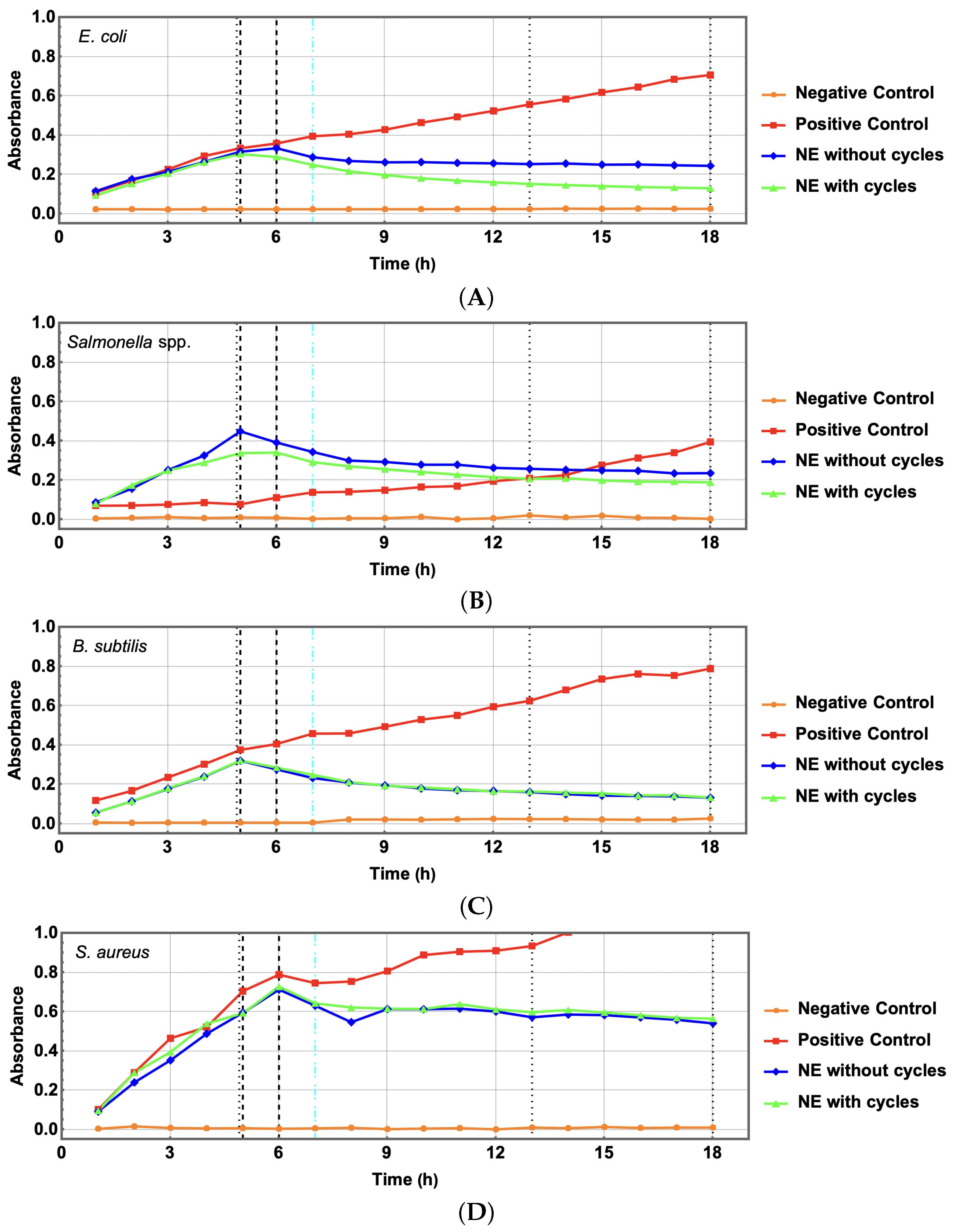
5.1. Comparative Antibacterial Effectiveness: Bacterial Growth Kinetics

The panels of Figure 13 summarise the complete study of bacterial kinetics considering OD at different hours of the experiment for (A) E. coli, (B) Salmonella spp., (C) B. subtilis, and (D) S. aureus (processed data corresponding to these figures are reported in Appendix C) in

Table A2. OD for Gram-negative bacteria: E. coli and Salmonella spp. for A, B, C, and D samples.

Bacteria	E. coli					Salmonella spp.
Hour	A	B	C	D		A	B	C	D
1	0.023	0.109	0.115	0.093		0.005	0.070	0.087	0.080
2	0.023	0.169	0.176	0.152		0.008	0.071	0.157	0.174
3	0.022	0.226	0.214	0.205		0.012	0.076	0.252	0.250
4	0.023	0.294	0.264	0.262		0.007	0.086	0.326	0.289
5	0.023	0.334	0.316	0.304		0.010	0.077	0.449	0.338
6	0.023	0.358	0.334	0.289		0.009	0.111	0.392	0.341
7	0.023	0.395	0.288	0.249		0.003	0.138	0.344	0.292
8	0.023	0.405	0.269	0.216		0.006	0.141	0.300	0.271
9	0.023	0.428	0.262	0.197		0.006	0.149	0.293	0.256
10	0.023	0.464	0.263	0.181		0.013	0.165	0.279	0.242
11	0.024	0.493	0.259	0.169		0.001	0.170	0.279	0.228
12	0.024	0.524	0.257	0.160		0.006	0.195	0.263	0.216
13	0.024	0.557	0.253	0.152		0.021	0.210	0.258	0.207
14	0.026	0.584	0.256	0.146		0.010	0.226	0.253	0.210
15	0.025	0.618	0.250	0.141		0.019	0.277	0.250	0.199
16	0.026	0.645	0.251	0.136		0.009	0.313	0.248	0.193
17	0.025	0.685	0.247	0.133		0.008	0.340	0.235	0.192
18	0.025	0.707	0.244	0.130		0.003	0.395	0.236	0.189

and

Table A3. OD for Gram-positive bacteria: B. subtilis and S. aureus for A, B, C, and D samples.

Bacteria	B. subtilis					S. aureus
Hour	A	B	C	D		A	B	C	D
1	0.007	0.119	0.057	0.057		0.004	0.102	0.092	0.096
2	0.005	0.168	0.115	0.115		0.016	0.290	0.240	0.289
3	0.006	0.235	0.178	0.180		0.008	0.465	0.353	0.395
4	0.006	0.302	0.239	0.241		0.006	0.522	0.488	0.539
5	0.006	0.375	0.320	0.321		0.007	0.705	0.595	0.593
6	0.006	0.405	0.276	0.285		0.004	0.789	0.713	0.728
7	0.006	0.458	0.232	0.248		0.006	0.746	0.631	0.643
8	0.022	0.459	0.209	0.212		0.009	0.754	0.547	0.622
9	0.022	0.493	0.194	0.193		0.002	0.807	0.614	0.616
10	0.021	0.529	0.180	0.184		0.005	0.889	0.613	0.614
11	0.023	0.551	0.171	0.175		0.007	0.906	0.616	0.639
12	0.025	0.595	0.167	0.166		0.001	0.911	0.601	0.612
13	0.024	0.625	0.162	0.165		0.010	0.935	0.572	0.598
14	0.024	0.680	0.151	0.159		0.007	1.005	0.586	0.609
15	0.022	0.736	0.144	0.155		0.013	1.050	0.583	0.596
16	0.021	0.762	0.142	0.145		0.008	1.090	0.571	0.582
17	0.021	0.754	0.140	0.145		0.010	1.104	0.559	0.569
18	0.027	0.789	0.133	0.134		0.010	1.165	0.541	0.565

. The negative control (orange line) corresponded to the nutrient broth as a cross-contamination control and to determine the influence of the pure nutrient broth on the OD of the samples. The positive control (red plot), which contained bacteria in nutrient broth, was used as a parameter to determine the proper growth of bacteria. The NE without cycles (blue line) was used to compare the efficacy of the NE with another NE with the same composition and concentration of EO that had been exposed to thermal cycles (green line). The black dashed lines correspond to the moments of addition of bacteria in the positive control and NE in the test flasks. In particular, the cyan dashed line indicates the precise moment when a saline solution was added to the positive control instead of the bacteria in order to compare it with the effect of the NE’s transparency. Finally, the observed dotted lines correspond to the specific times at which the samples were taken for the serial dilution tests.

In the case of Gram-negative bacteria (see Figure 13A), E. coli showed similar growth in all mediums until the fifth hour (when NEs were added), having an absorbance close to 0.3. The OD of the positive control continued to grow with time. In contrast, for both NEs, the OD increased until the NEs were added. After the addition of both NEs, the OD decreased, which can have two possible explanations. The first is related to the optical transparency of the NE, which, by its addition, reduced the overall turbidity of the system, thus modifying the OD measurement. However, the most predominant effect was the antibacterial properties of the NE that completely inhibited bacterial growth, as demonstrated by the CFU discussed below. The study of bacterial kinetics of Salmonella spp. (see Figure 13B) had a similar result as E. coli with the complete inhibition of bacteria. Before the addition of the NEs, the samples presented a considerably different OD of 0.449 in the sample without cycles and 0.338 for the sample corresponding to the NE with cycles. Despite these differences, both samples showed a reduction in absorbance caused by the effect of NEs on the microorganism.

The Gram-positive bacteria B. subtilis had results comparable to those previously observed in Gram-negative bacteria (see Figure 13C). The bacteria reached an absorbance of 0.3 before the incorporation of the NEs at the fifth hour. Both NE samples showed a progressive decay in the OD of the sample. This reduction after exposure to NE also indicated the effectiveness of the NEs against B. subtilis. It is relevant to mention that, as can be observed in Table A2 and Table A3 for B. subtilis, no increase in OD was observed after the addition of the NEs (C and D) starting from the sixth hour and decaying as time passed. This behaviour was consistent among these samples except for the S. aureus sample C, where the sample had a slight increase in its OD in the ninth hour and then started to decrease over time until the end of the experiment.

In fact, S. aureus exhibited a different behaviour from other microorganisms (see Figure 13D). The OD showed that S. aureus grew faster than the rest of the microorganisms analysed in the present study, reaching absorbances greater than 1.0 for the positive control and up to 0.7 for the other samples. Although an inhibitory effect was less prominent, it was attributed to different factors produced by the application of the NEs. As a result of the fast growth of the microorganism, proportional to the measured OD (almost twice that observed in the other microorganisms), a higher number of microorganisms were present in the sample.

We must consider that compared to the rest of the bacteria analysed in the present study, S. aureus presents a smaller size [53], which represents a higher concentration of bacteria in comparison. In fact, S. aureus has a size between 0.5 to 1 μm, compared with 2 to 6 μm long and a diameter of approximately 1 μm for B. subtilis, 1 to 2 μm long and about 0.5 μm in diameter for E. coli, and 2 to 5 μm long for Salmonella spp. [54,55,56,57]. Thus, both the OD and size of the bacteria imply a higher proportion of bacteria, which may have required a higher dose of NE for its complete inhibition. Another possible cause of a lower inhibitory effect is theorised to be the S. aureus’s morphology [58]. The bacteria previously studied present a bacillus morphology, whereas S. aureus has been reported to have a spherical morphology that aggregates in the form of grape-shaped clusters [53]. This particular bacterial arrangement may interfere with the permeability of the NEs.

5.2. Statistical Analysis of Meaningful Differences in OD for NE Treatments

The dataset for growth kinetics presented in Figure 13 is reported in Table A2 and Table A3 in Appendix C. Although differences between positive and negative controls with respect to NE treatments became evident, the differences between those two last different treatments were more subtle. Thus, we performed a two-factor ANOVA test followed by a Tukey post-test to detect meaningful differences between treatments using the NEs with or without thermal cycles, together with differences between hours during the experiment (after the sixth hour, when NEs were added for the first time). Thus, for the analysis, we considered the columns for samples C and D for hours 7 to 18 in Table A2 and Table A3. See the details in Appendix E.

The ANOVA test with a significance level of $\alpha =0.01$ showed significant differences between NEs and kinetic times for the four bacteria (in all cases, p-value was always lower than $\alpha$). For E. coli, Tukey’s post-test showed that the main differences were between the sixth hour and the remaining hours after the ninth. For Salmonella spp. and B. subtilis, the Tukey test detected meaningful differences throughout all consecutive hours, indicating a real antibacterial impact on kinetics but still differences between NEs with and without cycles. Tukey’s post-test for S. aureus set the differences mainly between the sixth hour and the subsequent ones, as graphically observed in Figure 13D.

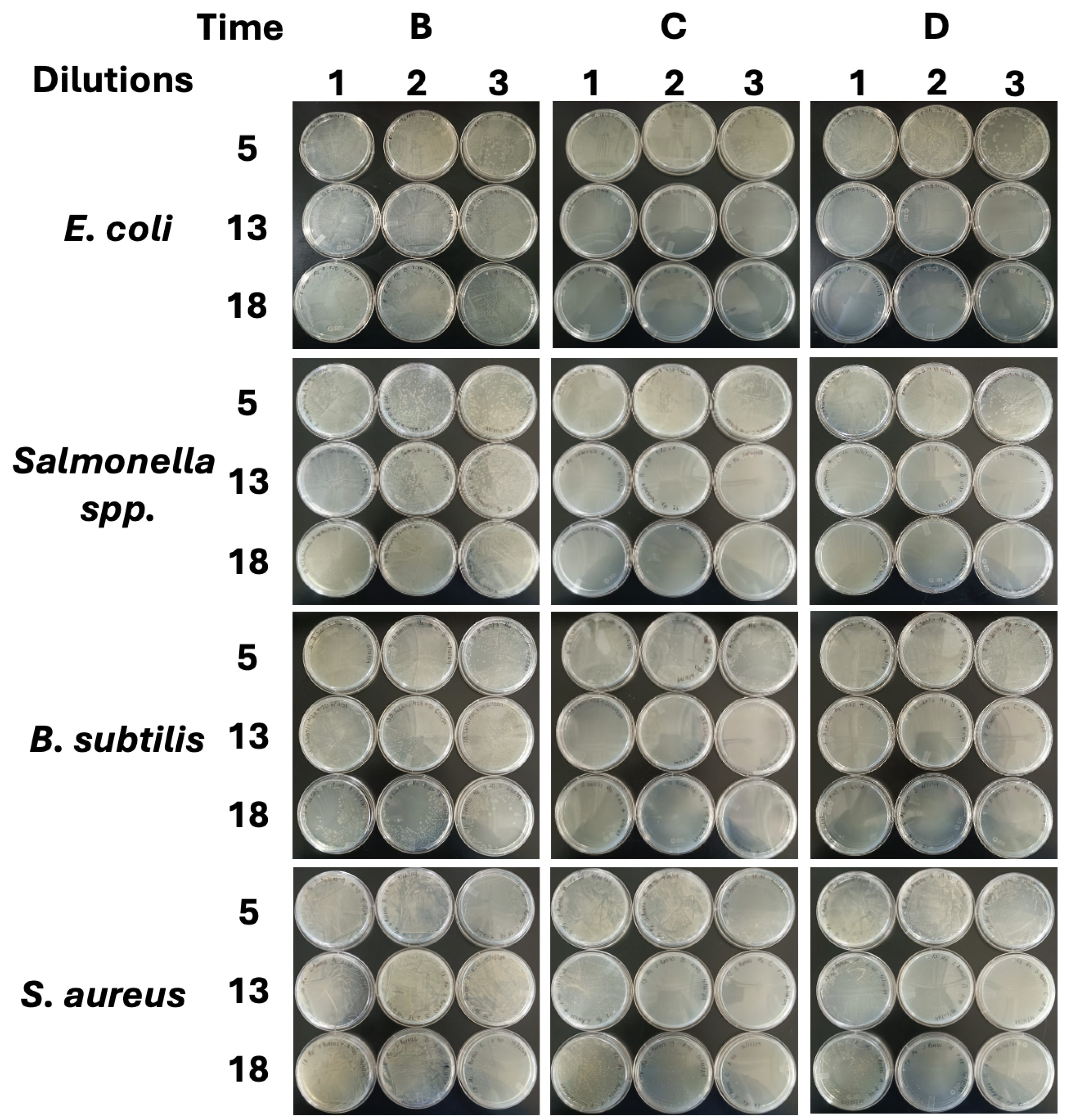
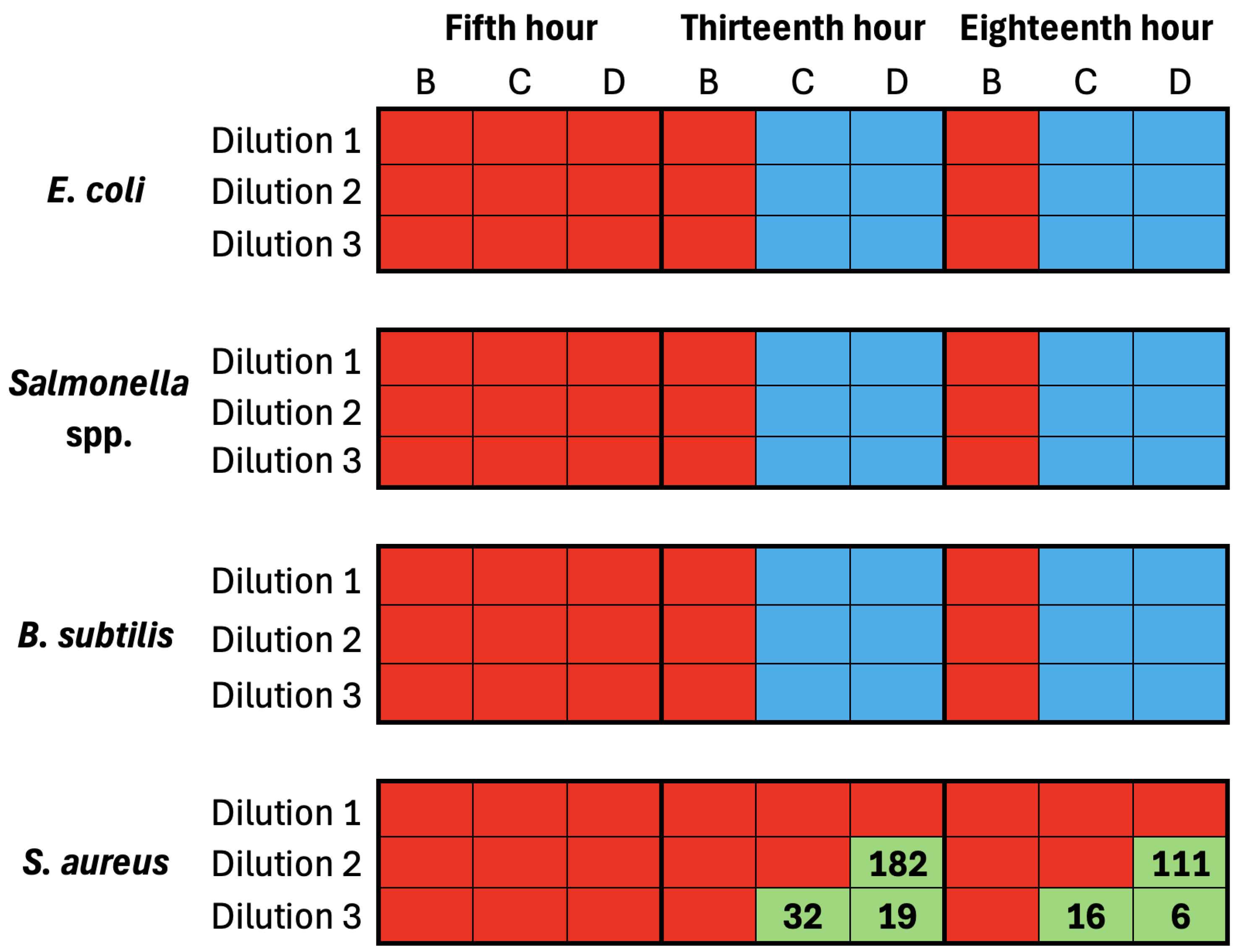
5.3. Comparative Antibacterial Effectiveness: Bacterial Colonies’ Counting

During the kinetic analysis of the bacterial growth, some samples were taken to perform serial dilutions and apply the diffusion technique. This technique was used to quantify the remaining bacteria after the addition of the NEs with the serial dilutions through the CFUs. Figure 14 summarises the results of diffusion in the Petri dish with the nutrient agar obtained for the different microorganisms. The dilutions were performed three times at a concentration of 1:10 while B, C, and D correspond to the positive control, the NE without heating–cooling cycles, and the NE with those cycles, respectively. The red squares correspond to samples with uncountable colonies, the green squares represent visible colonies with their respective count, and the blue squares correspond to plates where no CFUs grew. As expected, in each bacterium, every hour, the positive control (B) showed an uncountable number of colonies. In these cases, more dilutions would be required to determine the approximate CFUs present in the samples. In the thirteenth and eighteenth hour, the NEs had a complete inhibitory effect for E. coli, Salmonella spp., and B. subtilis even at low dilutions of the main samples, where a higher concentration of bacteria was expected, but as seen in Figure 14, there were no colonies present on the agar plate.

Although the NE had an inhibitory effect on S. aureus, it was not as high as for the rest of the microorganisms. The samples showed countable bacterial colonies in the second and third dilutions. Dilution 2 presented 182 and 111 colonies in the thirteenth and eighteenth hour in the NE with cycles. Likewise, dilution 3 presented 32 and 16 colonies for the NE without thermal cycles and 19 and 6 colonies in the NE with cycles. From the colonies counted on the agar plates, it was possible to approximate the number of bacteria present within the analysed sample per millilitre using (1) with $n=3$. In the analysis, only countable colony dilutions were considered, while others were considered outliers. Performing the corresponding calculations, the estimated value in the 13th hour was 32,000 CFU/mL, while for the 18th hour it was reduced to 16,000 CFU/mL for the NE without thermal cycles. However, in the case of the NE with cycles, approximately 18,600 CFU/mL were present in the 13th hour and 8550 CFU/mL for the 18th hour on average.

5.4. Discussion: Conserved Antibacterial Features

In antibacterial assays, we proved the efficacy of the NE even when exposed to thermal cycles. This was associated with the size stability of the NE droplets after these cycles. Furthermore, the NE was exposed to 37 °C during the kinetic growth study, a temperature at which the NE did not present considerable changes in its distribution, as demonstrated in the hysteresis analysis of NE. The size of the droplets played a key role in enhancing the antimicrobial activity of EO due to the increase in the surface area-to-volume ratio and therefore in the interactions between the NE and microorganisms [21]. Both NEs (before and after thermal cycles) showed bacterial inhibition against all bacterial strains, with the complete inhibition of E. coli, Salmonella spp., and B. subtilis. In particular, in S. aureus, there was no complete inhibition of the bacteria present in the nutrient broth, since its concentration at the fifth hour was considerably higher than that in the rest of the microorganisms. Although the bacteria were not completely inhibited, their concentration even at low dilutions implied a good inhibitory effect. There are many factors that are attributed to that difference in effectiveness. Although Gram-positive and Gram-negative classify bacteria into two main groups related to their cell wall, the morphology of microorganisms also plays an important role in their interactions. In particular, S. aureus is a coccus with a spherical shape of smaller size than E. coli, Salmonella spp. and B. subtilis instead present a bacilli shape. E. coli with sizes between 1 and 2 µm long and approximately 0.5 µm in diameter has been reported. Salmonellae have been reported with sizes ranging from 2 to 5 µm long and 0.5 to 1.5 µm in diameter. B. subtilis has been reported with a size of 2 to 6 µm long and a diameter of approximately 1 µm, while S. aureus has a size between 0.5 and 1 µm [54,55,56,57]. The smaller size of S. aureus could imply a higher surface area-to-volume ratio; however, this microorganism tends to form grape-type clusters, reducing the interaction of bacteria with the NE in general. The NE may have a greater inhibitory effect on the cells of the external bacteria of the cluster while reducing its efficacy for the internal bacteria.

6. Conclusions

In this particular study, we investigated an NE whose physical stability and antibacterial efficacy had previously been documented over a 1-year period. This time, its behaviour was analysed under a wider range of temperature variations to evaluate its potential commercial application in terms of the preservation of physical, chemical, and antibacterial properties. The results indicated a broadly stable physical behaviour within thermal cycles ranging from 10 °C to 50 °C, where nearly closed hysteresis cycles were observed, although differentiated during the heating and cooling phases. The parameters studied included the characteristic droplet size and the average size. Both processes exhibited non-linear and heterogeneous behaviour across different droplet sizes, suggesting greater alterations for larger droplets and increased stability for smaller droplets.

An observed phenomenon was that, although the average temperature of the sample remained constant, there were sustained dynamic processes internally that rearranged the droplet sizes in a differentiated manner, tending towards equilibrium in distribution over periods estimated at one hour. At the end of the cycles, an almost perfect return to the original distribution was observed, with minimal flocculation or clustering within the NE. This clustering appeared to occur at temperatures exceeding 40 °C, resulting in minimal distributions of larger droplets, which, given the operational limits of the DLS equipment, suggest this behaviour rather than flocculation or coalescence. Moreover, the chemical composition of the NE subjected repeatedly to these thermal cycles exhibited minimal variations, thus preserving its essential composition, particularly in volatile compounds thought to be responsible for its antibacterial properties, along with limited water evaporation. Consequently, the observed changes were not significant, indicating a low impact of the thermal cycles.

Furthermore, compared to the previous study, the antibacterial analysis was extended to compare its efficacy against two Gram-positive and two Gram-negative bacteria, in addition to more stringent antibacterial tests. All results demonstrated a preserved effect between the original NEs and those subjected to thermal cycling. The antibacterial efficacy, although observed, was reduced for Staphylococcus aureus but was not significantly affected by exposure to thermal cycles in the NE. Considering its environmentally friendly formulation and the safety of its components, the NE could serve as a viable alternative for addressing a variety of issues as a result of its inherent properties. These findings offer substantial confirmation of the stability of the NE, potentially paving the way for its application in multiple industries. For example, it may be used in sensing devices that require notable stability to temperature fluctuations or even as a comprehensive antimicrobial agent.

References

1. Mason, G.; Wilking, J.; Meleson, K.; Chang, C.; Graves, S. Nanoemulsions: Formation, structure, and physical properties. J. Phys. Condens. Matter 2006, 18, R635. [Google Scholar] [CrossRef]
2. Ozogul, Y.; Karsli, G.T.; Durmuş, M.; Yazgan, H.; Oztop, H.M.; McClements, D.J.; Ozogul, F. Recent developments in industrial applications of nanoemulsions. Adv. Colloid Interface Sci. 2022, 304, 102685. [Google Scholar] [CrossRef]
3. Weisany, W.; Yousefi, S.; Tahir, N.A.-R.; Golestanehzadeh, N.; McClements, D.J.; Adhikari, B.; Ghasemlou, M. Targeted delivery and controlled released of essential oils using nanoencapsulation: A review. Adv. Colloid Interface Sci. 2022, 303, 102655. [Google Scholar] [CrossRef]
4. Wang, Y.; Ai, C.; Wang, H.; Chen, C.; Teng, H.; Xiao, J.; Chen, L. Emulsion and its application in the food field: An update review. eFood 2023, 4, e102. [Google Scholar] [CrossRef]
5. Krishnamoorthy, R.; Athinarayanan, J.; Periasamy, V.S.; Adisa, A.R.; Al-Shuniaber, M.A.; Gassem, M.A.; Alshatwi, A.A. Antimicrobial activity of nanoemulsion on drug-resistant bacterial pathogens. Microb. Pathog. 2018, 120, 85–96. [Google Scholar] [CrossRef]
6. Dey, D.; Chowdhury, S.; Sen, R. Insight into recent advances on nanotechnology-mediated removal of antibiotic resistant bacteria and genes. J. Water Process. Eng. 2023, 52, 103535. [Google Scholar] [CrossRef]
7. Mba, I.E.; Nweze, E.I. Nanoparticles as therapeutic options for treating multidrug-resistant bacteria: Research progress, challenges, and prospects. World J. Microbiol. Biotechnol. 2021, 37, 108. [Google Scholar] [CrossRef]
8. Nazzaro, F.; Fratianni, F.; Martino, L.D.; Coppola, R.; Feo, V.D. Effect of Essential Oils on Pathogenic Bacteria. Pharmaceuticals 2013, 6, 1451–1474. [Google Scholar] [CrossRef]
9. Rodrigue, K.C.T.; Djouhou, M.C.; Koudoro, Y.A.; Dahouenon-Ahoussi, E.; Avlessi, F.; Koko, C.; Sohounhloue, D.; Simal-Gandara, J. Essential oils as natural antioxidants for the control of food preservation. Food Chem. Adv. 2023, 2, 100312. [Google Scholar] [CrossRef]
10. Santamarta, S.; Aldavero, A.C.; Ángeles Rojo, M. Antibacterial Properties of Cymbopogon martinii Essential Oil Against Bacillus subtillis Food Industry Pathogen. Proceedings 2020, 66, 1. [Google Scholar] [CrossRef]
11. Castro, J.C.; Pante, G.C.; de Souza, D.S.; Pires, T.Y.; Miyoshi, J.H.; Garcia, F.P.; Nakamura, C.V.; Mulati, A.C.N.; Mossini, S.A.G.; Junior, M.M.; et al. Molecular inclusion of Cymbopogon martinii essential oil with β-cyclodextrin as a strategy to stabilize and increase its bioactivity. Food Hydrocoll. Health 2022, 2, 100066. [Google Scholar] [CrossRef]
12. Wei, S.M.; Zhao, X.; Yu, J.; Yin, S.J.; Liu, M.J.; Bo, R.N.; Li, J.G. Characterization of tea tree oil nanoemulsion and its acute and subchronic toxicity. Regul. Toxicol. Pharmacol. 2021, 124, 104999. [Google Scholar] [CrossRef]
13. Qi, J.; Gong, M.; Zhang, R.; Song, Y.; Liu, Q.; Zhou, H.; Wang, J.; Mei, Y. Evaluation of the antibacterial effect of tea tree oil on Enterococcus faecalis and biofilm in vitro. J. Ethnopharmacol. 2021, 281, 114566. [Google Scholar] [CrossRef] [PubMed]
14. Lira, M.H.P.D.; de Andrade Júnior, F.P.; Moraes, G.F.Q.; da Silva Macena, G.; de Oliveira Pereira, F.; Lima, I.O. Antimicrobial activity of geraniol: An integrative review. J. Essent. Oil Res. 2020, 32, 187–197. [Google Scholar] [CrossRef]
15. Aljabri, N.M.; Shi, N.; Cavazos, A. Nanoemulsion: An emerging technology for oilfield applications between limitations and potentials. J. Pet. Sci. Eng. 2022, 208, 109306. [Google Scholar] [CrossRef]
16. McClements, D.J. Advances in edible nanoemulsions: Digestion, bioavailability, and potential toxicity. Prog. Lipid Res. 2021, 81, 101081. [Google Scholar] [CrossRef]
17. Czerniel, J.; Gostyńska, A.; Jańczak, J.; Stawny, M. A critical review of the novelties in the development of intravenous nanoemulsions. Eur. J. Pharm. Biopharm. 2023, 191, 36–56. [Google Scholar] [CrossRef]
18. Cox, S.D.; Mann, C.M.; Markham, J.L.; Gustafson, J.E.; Warmington, J.R.; Wyllie, S.G. Determining the Antimicrobial Actions of Tea Tree Oil. Mol. J. Synth. Chem. Nat. Prod. Chem. 2001, 6, 87. [Google Scholar] [CrossRef]
19. Maurya, A.; Singh, V.K.; Das, S.; Prasad, J.; Kedia, A.; Upadhyay, N.; Dubey, N.K.; Dwivedy, A.K. Essential Oil Nanoemulsion as Eco-Friendly and Safe Preservative: Bioefficacy Against Microbial Food Deterioration and Toxin Secretion, Mode of Action, and Future Opportunities. Front. Microbiol. 2021, 12, 751062. [Google Scholar] [CrossRef]
20. Gupta, S.; Chavhan, S.; Sawant, K.K. Self-nanoemulsifying drug delivery system for adefovir dipivoxil: Design, characterization, in vitro and ex vivo evaluation. Colloids Surfaces Physicochem. Eng. Asp. 2011, 392, 145–155. [Google Scholar] [CrossRef]
21. Mushtaq, A.; Wani, S.M.; Malik, A.R.; Gull, A.; Ramniwas, S.; Nayik, G.A.; Ercisli, S.; Marc, R.A.; Ullah, R.; Bari, A. Recent insights into Nanoemulsions: Their preparation, properties and applications. Food Chem. X 2023, 18, 100684. [Google Scholar] [CrossRef]
22. Ashaolu, T.J. Nanoemulsions for health, food, and cosmetics: A review. Environ. Chem. Lett. 2021, 19, 3381–3395. [Google Scholar] [CrossRef] [PubMed]
23. Sneha, K.; Kumar, A. Nanoemulsions: Techniques for the preparation and the recent advances in their food applications. Innov. Food Sci. Emerg. Technol. 2022, 76, 102914. [Google Scholar] [CrossRef]
24. Choi, S.J.; McClements, D.J. Nanoemulsions as delivery systems for lipophilic nutraceuticals: Strategies for improving their formulation, stability, functionality and bioavailability. Food Sci. Biotechnol. 2020, 29, 149–168. [Google Scholar] [CrossRef] [PubMed]
25. Gauthier, G.; Capron, I. Pickering nanoemulsions: An overview of manufacturing processes, formulations, and applications. JCIS Open 2021, 4, 100036. [Google Scholar] [CrossRef]
26. Jafari, S.; McClements, D. Nanoemulsions: Formulation, Applications, and Characterization; Elsevier Science: Amsterdam, The Netherlands, 2018. [Google Scholar]
27. Kumar, M.; Bishnoi, R.S.; Shukla, A.K.; Jain, C.P. Techniques for Formulation of Nanoemulsion Drug Delivery System: A Review. Prev. Nutr. Food Sci. 2019, 24, 225–234. [Google Scholar] [CrossRef]
28. Sánchez-Gaitán, E.; González-López, V.; Delgado, F. Polydispersity and composition stability in a long-term follow-up of palmarosa (Cymbopogon martini) and tea tree (Melaleuca alternifolia) O/W nanoemulsions for antibacterial use. Colloids Interfaces 2025, 9, 5. [Google Scholar] [CrossRef]
29. Carson, C.F.; Hammer, K.A.; Riley, T.V. Melaleuca alternifolia (Tea Tree) Oil: A Review of Antimicrobial and Other Medicinal Properties. Clin. Microbiol. Rev. 2006, 19, 50. [Google Scholar] [CrossRef]
30. Sanchez-Gaitan, E.J.; Rivero-Aranda, R.; Gonzalez-Lopez, V.; Delgado, F. Thermoresponsive test for a O/W Palmarosa Nanoemulsion: Dropletsize DLS, chemical composition FTIR and antibacterial test. Mendeley Data 2025. [Google Scholar] [CrossRef]
31. FDA Center for Drug Evaluation and Research. Inactive Ingredient Search for Approved Drug Products; U.S. Food & Drug Administration: Silver Spring, MD, USA, 2023.
32. Trefalt, G.; Szilágyi, I.; Borkovec, M. Schulze-Hardy rule revisited. Colloid Polym. Sci. 2020, 298, 961–967. [Google Scholar] [CrossRef]
33. Schulze, H. Schwefelarsen in wässriger Lösung. J. Prakt. Chem. 1882, 25, 431–452. [Google Scholar] [CrossRef]
34. Hardy, W.B.; Neville, F.H. A preliminary investigation of the conditions which determine the stability of irreversible hydrosols. Proc. R. Soc. Lond. 1900, 66, 110–125. [Google Scholar] [CrossRef]
35. Gupta, A.; Eral, H.B.; Hatton, T.A.; Doyle, P.S. Nanoemulsions: Formation, properties and applications. Soft Matter 2016, 12, 2826–2841. [Google Scholar] [CrossRef] [PubMed]
36. Yi, L.; Wang, C.; van Vuren, T.; Lohse, D.; Risso, F.; Toschi, F.; Sun, C. Physical mechanisms for droplet size and effective viscosity asymmetries in turbulent emulsions. J. Fluid Mech. 2022, 951. [Google Scholar] [CrossRef]
37. Gupta, A.; Eral, H.B.; Hatton, T.A.; Doyle, P.S. Controlling and predicting droplet size of nanoemulsions: Scaling relations with experimental validation. Soft Matter 2016, 12, 1452–1458. [Google Scholar] [CrossRef]
38. Beal, J.; Farny, N.G.; Haddock-Angelli, T.; Selvarajah, V.; Baldwin, G.S.; Buckley-Taylor, R.; Gershater, M.; Kiga, D.; Marken, J.; Sanchania, V.; et al. Robust estimation of bacterial cell count from optical density. Commun. Biol. 2020, 3, 512. [Google Scholar] [CrossRef]
39. Mira, P.; Yeh, P.; Hall, B.G. Estimating microbial population data from optical density. PLoS ONE 2022, 17, e0276040. [Google Scholar] [CrossRef]
40. Reynolds, J. Serial Dilution Protocols. Am. Soc. Microbiol. 2005, 2005, 1–7. [Google Scholar]
41. Sanders, E.R. Aseptic Laboratory Techniques: Plating Methods. J. Vis. Exp. 2012, 63, e3064. [Google Scholar] [CrossRef]
42. Kumar, N.; Verma, A.; Mandal, A. Formation, characteristics and oil industry applications of nanoemulsions: A review. J. Pet. Sci. Eng. 2021, 206, 109042. [Google Scholar] [CrossRef]
43. Tukey, J.W. Comparing Individual Means in the Analysis of Variance. Biometrics 1949, 5, 99–114. [Google Scholar] [CrossRef]
44. Scarlett, B. (Ed.) Spectroscopy. In Particle Characterization: Light Scattering Methods; Springer: Dordrecht, The Netherlands, 2002; pp. 223–288. [Google Scholar] [CrossRef]
45. Ross Hallett, F. Scattering and Particle Sizing Applications. In Encyclopedia of Spectroscopy and Spectrometry, 2nd ed.; Lindon, J.C., Ed.; Academic Press: Oxford, UK, 1999; pp. 2488–2494. [Google Scholar] [CrossRef]
46. Malvern Instruments Ltd. Zetasizer Nano User Manual; Malvern Instruments Ltd.: Worcestershire, UK, 2013. [Google Scholar]
47. Goddeeris, C.; Cuppo, F.; Reynaers, H.; Bouwman, W.; Van den Mooter, G. Light scattering measurements on microemulsions: Estimation of droplet sizes. Int. J. Pharm. 2006, 312, 187–195. [Google Scholar] [CrossRef]
48. Gupta, A.; Narsimhan, V.; Hatton, T.A.; Doyle, P.S. Kinetics of the Change in Droplet Size During Nanoemulsion Formation. Langmuir 2016, 32, 11551–11559. [Google Scholar] [CrossRef]
49. Peng, F.; Ke, Y.; Lu, S.; Zhao, Y.; Hu, X.; Deng, Q. Anion amphiphilic random copolymers and their performance as stabilizers for O/W nanoemulsions. RSC Adv. 2019, 9, 14692–14700. [Google Scholar] [CrossRef] [PubMed]
50. Oliveira, A.E.; Duarte, J.L.; Cruz, R.A.; da Conceição, E.C.; Carvalho, J.C.; Fernandes, C.P. Utilization of dynamic light scattering to evaluate Pterodon emarginatus oleoresin-based nanoemulsion formation by non-heating and solvent-free method. Rev. Bras. Farmacogn. 2017, 27, 401–406. [Google Scholar] [CrossRef]
51. Ee, S.L.; Duan, X.; Liew, J.; Nguyen, Q.D. Droplet size and stability of nano-emulsions produced by the temperature phase inversion method. Chem. Eng. J. 2008, 140, 626–631. [Google Scholar] [CrossRef]
52. Marinković, J.; Bošković, M.; Tasić, G.; Vasilijević, B.; Marković, D.; Marković, T.; Nikolić, B. Cymbopogon martinii essential oil nanoemulsions: Physico-chemical characterization, antibacterial and antibiofilm potential against Enterococcus faecalis. Ind. Crop. Prod. 2022, 187, 115478. [Google Scholar] [CrossRef]
53. Zhou, S.; Rao, Y.; Li, J.; Huang, Q.; Rao, X. Staphylococcus aureus small-colony variants: Formation, infection, and treatment. Microbiol. Res. 2022, 260, 127040. [Google Scholar] [CrossRef]
54. Baron, S. Medical Microbiology, 4th ed.; University of Texas Medical Branch at Galveston: Galveston, TX, USA, 1996. [Google Scholar]
55. Errington, J.; van der Aart, L.T. Microbe Profile: Bacillus subtilis: Model organism for cellular development, and industrial workhorse. Microbiology 2020, 166, 425–427. [Google Scholar] [CrossRef]
56. Riley, M. Size Limits of Very Small Microorganisms: Proceedings of a Workshop; National Academies Press: Washington, DC, USA, 1999. [Google Scholar]
57. Drepper, F.; Biernat, J.; Kaniyappan, S.; Meyer, H.E.; Mandelkow, E.M.; Warscheid, B.; Mandelkow, E. A Combinatorial Native MS and LC-MS/MS Approach Reveals High Intrinsic Phosphorylation of Human Tau but Minimal Levels of Other Key Modifications. J. Biol. Chem. 2020, 295, 18213–18225. [Google Scholar] [CrossRef]
58. Parastan, R.; Kargar, M.; Solhjoo, K.; Kafilzadeh, F. Staphylococcus aureus biofilms: Structures, antibiotic resistance, inhibition, and vaccines. Gene Rep. 2020, 20, 100739. [Google Scholar] [CrossRef]
Figure 1. Tests integrated in this research to analyse the thermoresponsive effect of the NE together with the associated methods.
Colloids 09 00047 g001
Figure 2. Droplet size distributions in a log-scale (horizontal axis in nm ) obtained for a series of temperatures 10.0 , 12.5 , 15.0 , , 50.0   ° C in agreement with the colour bar at the top (blue, the coldest, and red, the hottest). Measurements were obtained every two minutes with (A) ascending, and (B) descending temperatures. The nearest body temperature (37.5 °C) is highlighted with a dashed black line. The inset on the left reveals emergent distributions for larger droplet sizes.
Colloids 09 00047 g002
Figure 3. Droplet size distributions in a log-scale (horizontal axis in nm ) obtained for a series of temperatures 10 , 20 , , 50   ° C in agreement with the colour bar at the top (blue, the coldest, and red, the hottest). Measurements were obtained every five minutes with (A) ascending, and (B) descending temperatures. The inset on the left reveals emergent distributions for larger droplet sizes.
Colloids 09 00047 g003
Figure 4. Droplet size distributions in a log-scale (horizontal axis in nm ) obtained for a series of temperatures 10 , 20 , , 50   ° C in agreement with the bar colour at the top (blue, the coldest, and red, the hottest). Measurements were obtained every twenty minutes with (A) ascending, and (B) descending temperatures. The inset on the left reveals emergent distributions for larger droplet sizes.
Colloids 09 00047 g004
Figure 5. Thermal cycle of heating and cooling for a 2 min waiting time before measurement (Figure 2). The horizontal axis reports the temperature and vertical one the (A) maximum diameter distribution, d m a x (peak), and (B) mean diameter, d m e a n , both including error bars for the three-fold experiment. PDI = σ / μ is reported in colour in agreement with the bar at the top. Droplet size dispersion σ d is reported by the dot size barely in agreement with the legend in the upper-left scale. The red dashed line marks the body temperature, 37.5°C.
Colloids 09 00047 g005
Figure 6. Corresponding thermal cycle of heating and cooling for 5 min of waiting. Vertical axis reports (A,B) the maximum diameter distribution, d m a x , and (C,D) the mean diameter, d m e a n . Each paired plot first shows a closer view at lower temperatures and then a complete view, respectively. Previous elements from Figure 5 were preserved.
Colloids 09 00047 g006
Figure 7. Corresponding thermal cycle of heating and cooling for 20 min of waiting. Vertical axis reports (A,B) the maximum diameter distribution, d m a x , and (C,D) the mean diameter, d m e a n . Each paired plot first shows a closer view at lower temperatures and then a complete view, respectively. Previous elements from Figure 5 were preserved.
Colloids 09 00047 g007
Figure 8. Droplet size distributions in a log-scale (horizontal axis in nm ) during stabilisation at constant temperature after (A) raising the temperature from 18 °C (lab temperature) to 30 °C, and after (B) lowering the temperature back to 18 °C. Measurements performed at 0 , 1 , 11 , 21 , , 61 min (temperature transition reached in the first minute) in agreement with the bar colour. The inset on the left reveals emergent distributions for larger droplet sizes.
Colloids 09 00047 g008
Figure 9. Droplet size distributions in a log-scale (horizontal axis in nm ) during stabilisation at constant temperature after (A) raising the temperature from 18 °C (lab temperature) to 40 °C, and after (B) lowering the temperature back to 18 °C. Measurements performed at 0 , 1 , 11 , 21 , , 61 min (temperature transition reached in the first minute) in agreement with the bar colour. The inset on the left reveals emergent distributions for larger droplet sizes.
Colloids 09 00047 g009
Figure 10. Droplet size distributions in a log-scale (horizontal axis in nm ) during stabilisation at constant temperature after (A) raising the temperature from 18 °C (lab temperature) to 50 °C, and after (B) lowering the temperature back to 18 °C. Measurements performed at 0 , 1 , 11 , , 61 min (temperature transition reached in the first minute) in agreement with the bar colour. The inset on the left reveals emergent distributions for larger droplet sizes.
Colloids 09 00047 g010
Figure 11. Graphic representation for the droplet size distribution dynamics as a function of heating. Blue distributions correspond to the initial and red ones to the final distributions at the equilibrium. Additional modes appear during the process. Note the natural oscillations in the main peak (vertical arrows in respective colours).
Colloids 09 00047 g011
Figure 12. FTIR of the main bands present in (A) the raw materials and the NE before the thermoresponsive cycles and (B) comparison of the NE before and after the thermoresponsive cycles to evaluate changes in the composition of the original NE.
Colloids 09 00047 g012
Figure 13. Time-dependent growth kinetics of bacterial strains reported through OD (reported as the relative absorbance) for (A) E. coli, (B) Salmonella spp., (C) B. subtilis, and (D) S. aureus, considering a negative control (nutrient broth, orange), a positive control (nutrient and microorganisms, red), NE without thermal cycles in nutrient and microorganisms (blue), and NE with thermal cycles nutrient and microorganisms (green). They include the addition of inocula and NEs (black dashed line), addition of a saline solution and NEs (cyan dashed line), and samples’ storage for the serial dilutions (black dotted lines).
Colloids 09 00047 g013
Figure 14. Bacterial growth observations over time at the fifth, thirteenth, and eighteenth hours where the red sections correspond to uncountable plates, blue sections correspond to the absence of microorganisms caused by the NEs, and green sections correspond to countable bacterial colonies with their respective count.
Colloids 09 00047 g014