1. Introduction
Bubble Visualisation Techniques
Bubbles ranging from (1 µm–1000 µm) in size are termed microbubbles. Although the actual definition of a microbubble depends on its application, for the purposes of this study, the aforementioned definition holds [
1]. Bubbles have been visualised for over half a millennia with Newton’s observation of bubble formation with a pair of lenses, whilst the Berthelot tube method has long been known as a way to observe cavitation in liquids [
2]. Reynolds discovered bubble formation by cavitation via the process of boiling [
3]. Bubble visualisation is easier for fine bubbles or for sparse microbubbles generated by either energy intensive or low throughput methods. Single bubbles can be simply studied via a microscope or a lens. Characterising cloud bubble dynamics is more problematic. Common practice is to use optical imaging coupled with the volume fraction of the bubble by juxtaposing a control image (bubble-free) over the bubble cloud image, followed by using pixel data and a Hough transform to determine the void fraction. However, this does not necessarily provide any more information about the bubble size distribution (BSD). Therefore, optical methods were developed with algorithms relying on variety of techniques to estimate bubble sizes [
4,
5,
6,
7,
8,
9,
10,
11]. Interests in bubble cloud dynamics are largely focused on marine engineering and oceanic sciences. This is due to the high cost of producing microbubbles, thereby opposing the use of microbubbles for industrial purposes.
Fluidic oscillation offers substantial reduction in energy costs for generating microbubbles with concomitant increase of throughput [
12]. The Tesař–Zimmerman fluidic oscillator [
13]—a modified version of the feedback loop type oscillator—made it possible to use microbubbles economically for industrial applications with several applications explored for lab-scale [
14] and large-scale industrial purposes. Several T-Junction devices [
15,
16] and sonication [
17], amongst other techniques can now be used for generating a cloud of microbubbles with a wide size distribution. With the advent of such techniques, the methods for visualisation have simultaneously shifted from direct measurement using a microscope to indirect techniques for higher accuracy through the exploitation of properties exhibited by bubbles. The BSD depend on the methods used for obtaining the bubble size and the statistical analyses that accompany these methods. Methods used for inferring BSD include four-point optical probe [
18,
19,
20,
21], capacitance probes [
22], electrical conductivity [
23], video imaging [
24,
25,
26,
27], acoustical backscatter [
28], acoustic resonator [
29], acoustic pulse propagation sensor [
29], laser diffraction [
30], acoustic attenuation [
31,
32,
33], University of Capetown Technique (UCT) bubble size sampler [
34] and laser attenuation [
35].
Several comparison studies have been performed on bubble visualization, such as [
5], as well as work on resolving optical and acoustic methods [
29,
36,
37] in order to merge the understanding of these techniques and try to obtain a better understanding of these visualisation systems. However, comparison studies for cloud bubble dynamics with an emphasis on detecting smaller bubbles have not been performed, nor studied in detail.
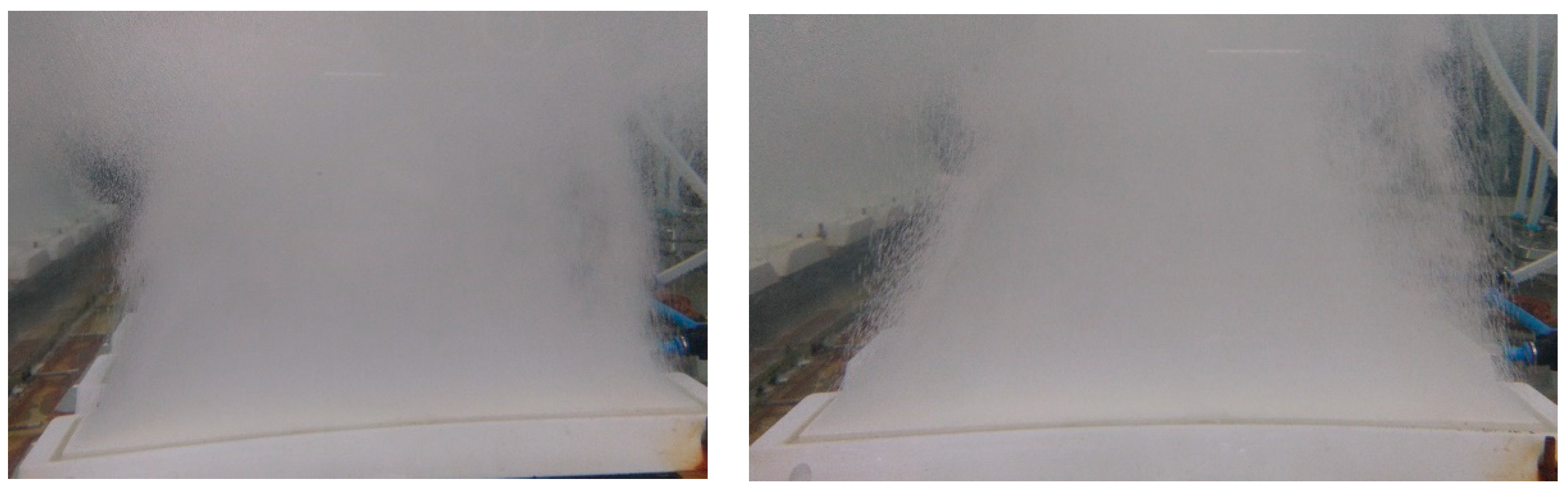
Additionally, visual inspection, as can be seen in
Figure 1, show that for microbubble clouds, visual inferences cannot be made and size distributions need to be carefully obtained and analysed.
Statistical analyses performed on the sizing by each method skews the size distribution and therefore the final average bubble size obtained could be quite different depending on the actual statistical analysis applied. A comparison study is performed for three classes of bubble sizing techniques, including optical, laser diffraction, and acoustic. Specifically, Dynaflow’s Acoustic Bubble Spectrometer (ABS), Malvern Instruments’ SprayTec, and high-speed photography (Photron FastCam S3). Each method offers its own advantages and disadvantages depending on the actual method of estimating the bubble size population.
We test the hypothesis that for measuring a bubble cloud, an acoustic method is likely the method most representative of the cloud. There is a possibility that larger bubbles obscure the smaller bubbles in the cloud for the other methods. The other methods require a small sampling window/volume to garner the cloud information, which may also hamper their performance.
This section discusses the distinct advantages offered by the different visualisation methods and other capabilities.
2. Optical Methods
This is a direct form of measurement and visualisation, as well as the simplest method since it is a quick and easy way to infer the BSD.
High-Speed Photography
Optical methods usually involve a monochromatic light source and require the liquid to be transparent to light. The greater the contrast between the bubble and the background, the more robust it is for automated image analysis. High-speed photography is commonly used due to its ease of use. Most high-speed cameras have the ability to capture more than 500 frames per second (fps).
The bubble generator is placed in the centre with the light source and the camera placed opposite each other in order to obtain the best contrast for the bubbles. Automated image analysis is made easier if there is a good contrast between the background and the bubbles. The camera need not be able to capture more than 2000 fps to obtain a BSD. The simplicity of the system is one of its key advantages and significantly reduces the costs of the system. Automated image analysis is possible by simple algorithms by using any suitable programming language viz. Octave, ImageJ, MATLAB, Mathematica, and LabView.
Image analysis can also be performed manually. It can, therefore, provide bubble sizes without the need of computing power (albeit a cumbersome approach). Although this technique is convenient for single bubbles, cloud bubble dynamics present their own drawbacks. Automated image analysis cannot be reliably used for overlapping bubbles, noncircular bubbles, and near-wall bubbles (the bubbles also need to be in a single plane). Depending on the angle used, the bubble size obtained is significantly different. A long working focal length lens could be used (to ensure wall effects are minimised) but makes the process more expensive and cumbersome.
This problem can be solved by using multiple cameras at the three focal planes but results in the need to develop a way to accrue synchronised information from the three cameras and then collate the information together in order to obtain a bubble spectrum. Bubbles at the wall, partial bubbles, noncircular (spherical for the 3D system) are not detected by automated image analysis. These features makes the task tedious and cumbersome, while introducing inference errors.
Different lenses are required for a particular size range. They cannot be used simultaneously unless another camera is used. A comprehensive BSD is therefore difficult to obtain, so only a certain size range is observed at a given time. Once the appropriate lens has been chosen and the camera focused, it cannot detect the other bubble size ranges and cannot differentiate between the particles and bubbles if they are too small. Multiple lenses increase the cost of the system, the number of measurements, and the required analyses and comparisons.
A number of additional analyses can be made using a high-speed camera. If the camera has a high frame rate, such as the Photron FastCam S3, the rise velocity of the bubble can be measured as well as bubble formation dynamics, growth dynamics, conjunction and coalescence. Adil et al. [
38] presents image analysis techniques for the rise velocity of a system with an ordinary camera.
3. Acoustic Methods
Acoustic methods have been used for bubble sizing for almost half a century. Excellent reviews on bubble sizing using acoustic methods have been compiled [
39]. Bubble acoustic responses include backscatter, attenuation, resonance and sound speed modulations in the medium [
32]. This is made possible as a result of the substantial effect that a bubble has on the propagation of acoustic waves.
A significant advance to demonstrate acoustic determination of the bubble sizes for bubble clouds was made in 1989 [
40].
The relationship between complex sound speed in a bubbly medium (c
m), and bubble free sound speed (c
0), is defined by
a is the bubble radius(m),
f is the insonant frequency (Hz),
fR is the natural frequency of the bubble of size
a, n(
a) is the bubble density function and
δ is bubble damping magnitude.
This relationship by itself can be used for obtaining bubble size. However, there is a loss in fidelity, which is why other methods have been adopted for development. This along with the relation:
where
u(f) is speed and phase speed (
v(f)) is given by:
And attenuation constant α is given by:
This combination provides the bubble with a resonant frequency at which to oscillate. According to the solution of the Rayleigh–Plesset equation, the linear response of the bubble under continuous insonation and its nonlinear response, along with oscillation, is a property that is observed only for bubbles (not particles). These properties make this method favoured due to its specificity.
Also, in the Rayleigh region, the insonation frequency is dependent on the sixth power of the radius thereby making it a highly specific method.
Several authors [
41,
42,
43,
44,
45,
46,
47,
48,
49,
50,
51] have used hydrophones to infer bubble size, deploying these different properties in order to obtain BSD for coated (polymeric shells/protein shells, liposomes) and uncoated (clear interface) bubbles.
The drawback comes in the form of the complicated inversion observed due to the inverse of the ill posed Fredholm integral [
52], which results in an enlarged effect on the solution from small measurement errors.
Acoustic Bubble Spectrometry (ABS) by Dynaflow
Acoustic bubble spectrometry (ABS), used in this study is based on an assumption known as the resonant bubble approximation (RBA). The system and the algorithm used for the bubble size measurement is described well by [
53].
The main development made by Dynaflow is the algorithm based on constrained minimisation. A hydrophone is a microphone that can be used underwater. As sound travels much faster in water and attenuates slower than with air as the medium, the design of the hydrophone has to be modified accordingly by matching its acoustic impedance in water [
3]. An equiresponsive hydrophone pair is used in this system with one utilised for generation and the other for the detection.
Microbubbles oscillate linearly upon ultrasonic insonation. If the mechanical index of the insonation ultrasound is high enough, the oscillations become nonlinear, increasing the specificity, hence more effective for sizing. The acoustic pressure has to be increased to be able to cause a nonlinear response and a compression or expansion, which results in the emissions of nonlinear signals and their respective harmonics of the transmitted signal. This also causes the acoustic impedance of the bubble to change with respect to water, improving the signal. This can be thought of as a contrast enhancing effect of the coating on a coated medical microbubble.
Initially the two hydrophones are placed opposite each other with the bubble generator placed in the centre. The transmitter insonates starting from a specific frequency and performs a frequency sweep. This signal may or may not be amplified depending on the conditions. Whilst the receiver amplifies the signal, the data obtained is then inverted by bespoke software provided by the company. A zero calibration reading is taken (P0 - analogous to any spectroscopic method). The production of bubbles causes a change in pressure when the bubble cloud is insonated. This change is recorded by the transducers and compared to the zero calibration reading.
The ABS (
Figure 2) provides continuous, real time bubble size distribution that are extremely specific to bubbles. Using an optimised octophonic system (four pairs of hydrophones), a comprehensive size distribution, between 10 µm and 2 mm. Void fractions of down to 3 × 10
−3 [
53], can be measured and verified whilst conducting this study.
Skewed results are obtained if bubbles stick to the surface of the hydrophones. Since the hydrophones need to be submerged in the liquid, even small imperfections act as large centres for bubble coalescence. Therefore, the hydrophones need to be regularly wiped and cleaned using water [
54].
The distinct advantage of acoustic spectrometry over laser diffraction and optical methods is that bubbles in liquids are more transparent to acoustic waves than to light waves [
36].
ABS can also be used to measure the sound speed of the medium and therefore determine the viscosity or density of the medium.
4. Photonic Methods
Photonic methods are most commonly used in particle sizing aside from optical imaging. Photonic methods are incredibly effective in terms of accuracy and range of the size distributions for small samples. The accuracy of photonic methods reduces for bubbles relative to particles not only due to the immanent property of the bubble but also due to total internal reflection that occurs upon illumination (presuming particles are opaque). Bubble opacity is not high so that the diaphanous behaviour exhibited by the bubbles affects the laser diffraction and scattering. Particles and bubbles interact with light (and sound) in three ways: absorption, emission and scattering. Assuming that the particles are spherical, the intensity of the scatter is measured and the BSD is inferred using Mie theory (assuming a noninteracting bubble cloud population). The scatter is dependent on the size of the particles, whilst the intensity is dependent on the number of particles. A bubble can be thought of as a dielectric sphere. An air filled bubble, with water as a medium, fits into this category. Mie theory describes diffraction, refraction and reflection (internal and external). Diffraction cannot tell the difference between a particle and bubble since it is independent of particle properties. Conversely, refraction and reflection are dependent on the type of particle and its refractive index. The refractive index, however, is fairly difficult to measure effectively. When light passes through a particle with an angle of incidence = 0⁰, there is no change to the incident light. However, at all the other angles the three effects can be observed depending on the angle of incidence. Total internal reflection is observed for incident angles above the critical angle. Several devices used for particle sizing using photonic methods have been reviewed [
30].
Malvern SprayTec
According to Malvern Instruments, SprayTec uses dynamic light scattering (DLS) as a principle, and has a range with the 300 mm lens) between 0.1–900 µm (D
x(50): 0.5–600µm). The system measures droplet size distributions and requires the angular intensity of light scattered from a spray to be measured as it passes through a laser beam (based on transmittance and scattering). This scattering pattern is first recorded and then analysed using Fraunhofer and Mie scattering to yield a size distribution. Complete resolution of the size dispersion has been obtained through optimisation as well as using a patented multiple scattering algorithm ensuring up to 98% obscuration [
55].
Figure 3 shows a schematic of the SprayTec system. Two lasers, with collimating optics, are placed opposite each other with the test cell placed in the centre so that a small area of interest is measured. This was a modification made to the original setup as the usual method for measurement is spraying it in the space between the two lasers. The receiving lens adjusts itself—a self-correcting calibration system for alignment, which is critical for this measurement technique, and accounts for major errors and inconsistencies. This has been taken into account by the manufacturer by incorporating a separate collimator and an auto alignment feature embedded.
The modification made here is to use a glass cell for bubble measurement while using a macro provided by Malvern Instruments to account for changes in refractive index.
Bubbles are droplets with the phases inverted. Therefore, the SprayTec can be used for bubble size measurements especially for obtaining high density BSD [
13,
56].
Cloud bubble sizing might be a difficult phenomenon for laser diffraction techniques since the bubbles diffract far more than a particle with possibility of total internal reflection in a bubble. Since this principle depends on light diffraction and not a property exhibited specifically by bubbles alone, it cannot differentiate between bubble or particle. It is also affected by the diffractions caused by bubbles and particles in its vicinity and therefore some bubbles might be ‘hidden’. Photonic methods depend on the liquid being transparent to the wavelength of light but need not be transparent in the visible region. This gives an advantage to the photo-acoustic methods over optical methods.
Arguably, there are fewer assumptions to be made for photonic methods, compared to acoustic methods for function inversion (a laser is essentially a monochromatic point source whereas the insonation frequency is not as monodisperse). However, it is the inversion of the same ill-posed Fredholm integral that makes this problem difficult [
57].
One of the simplest theories used in particle sizing through laser diffraction is the Fraunhofer approximation. This model predicts the scattering pattern that is created when a solid, opaque disc of a known size is passed through a laser beam. This means that it is imperative that the transmission of light through the particle is assumed to be zero. For a bubble, that never happens. This model is satisfactory for large particles (over 50-μm diameter) but it does not describe the scattering exactly. The Fraunhofer approximation is no longer used due to the assumptions, which do not necessarily hold true for particles. However, they do hold true for bubbles.
The particle is much larger than the wavelength of light employed. ISO 13320:2009 defines this as being greater than 40 times the wavelength of incident light (i.e., 25 μm when a He-Ne laser is used). The other approximation is that all sizes of particle scatter with equal efficiencies. That is not true, since bubbles scatter more than particles and a bubble is not opaque.
It is for the above reasons that Mie theory is utilised; all the particles are spherical. For bubbles smaller than 1 mm, this approximation holds and is also used for the RBA assumption used in the ABS.
However, refractive indices for the material, medium and the absorption part of the refractive index must be known or estimated. These can be estimated for most substances and for bubbles—a comparatively a simpler prospect. Work has been conducted to demonstrate that laser diffraction is not very effective for obtaining cloud BSD [
5]. Statistical methods need to be discussed since they are used in conjunction with any indirect forms of bubble size measurement.
5. Statistical Analyses
Size distributions are expressed in terms of number averages (simple average based on the number of bubbles) and void fraction averages (based on the volume occupied by the bubbles).
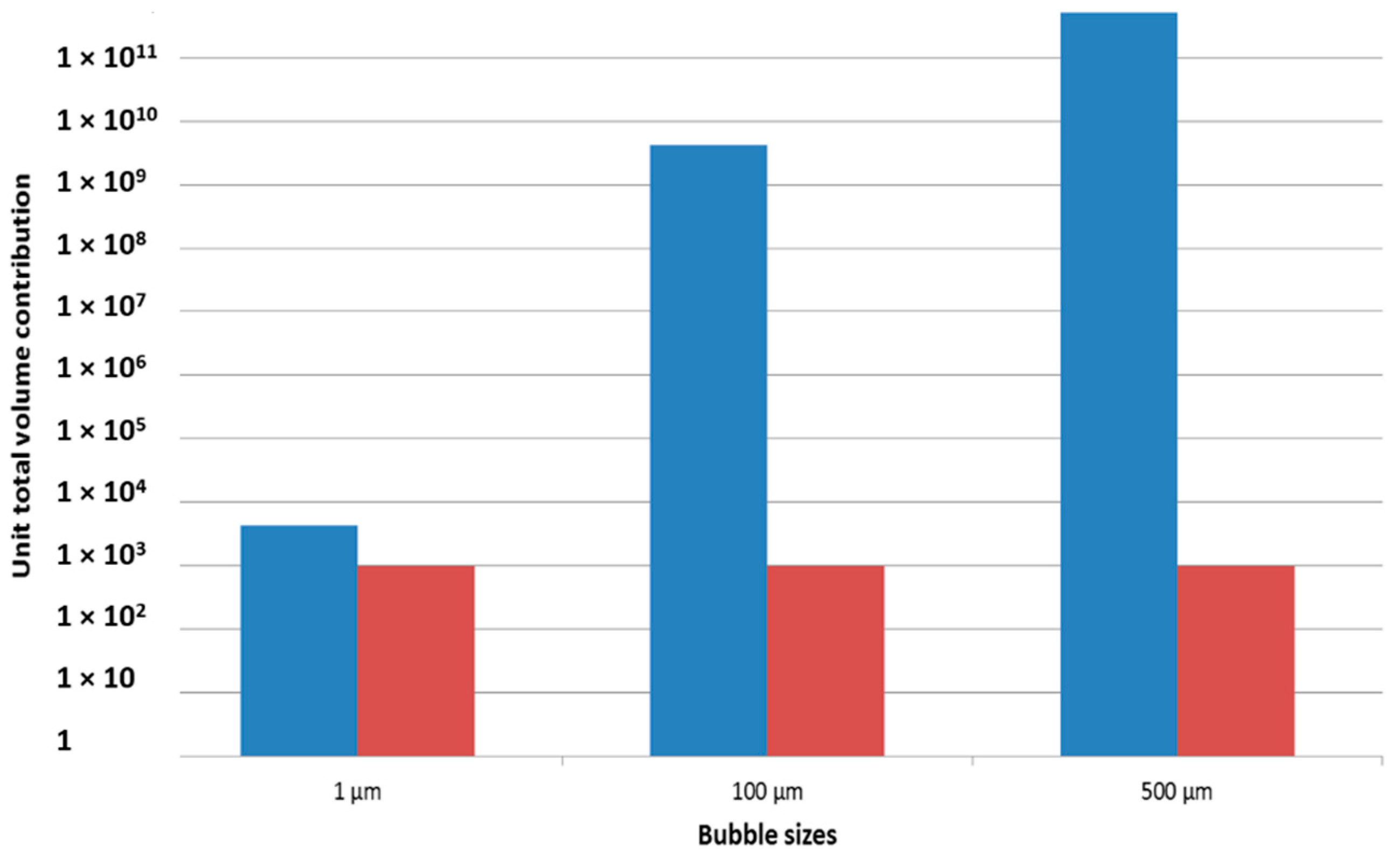
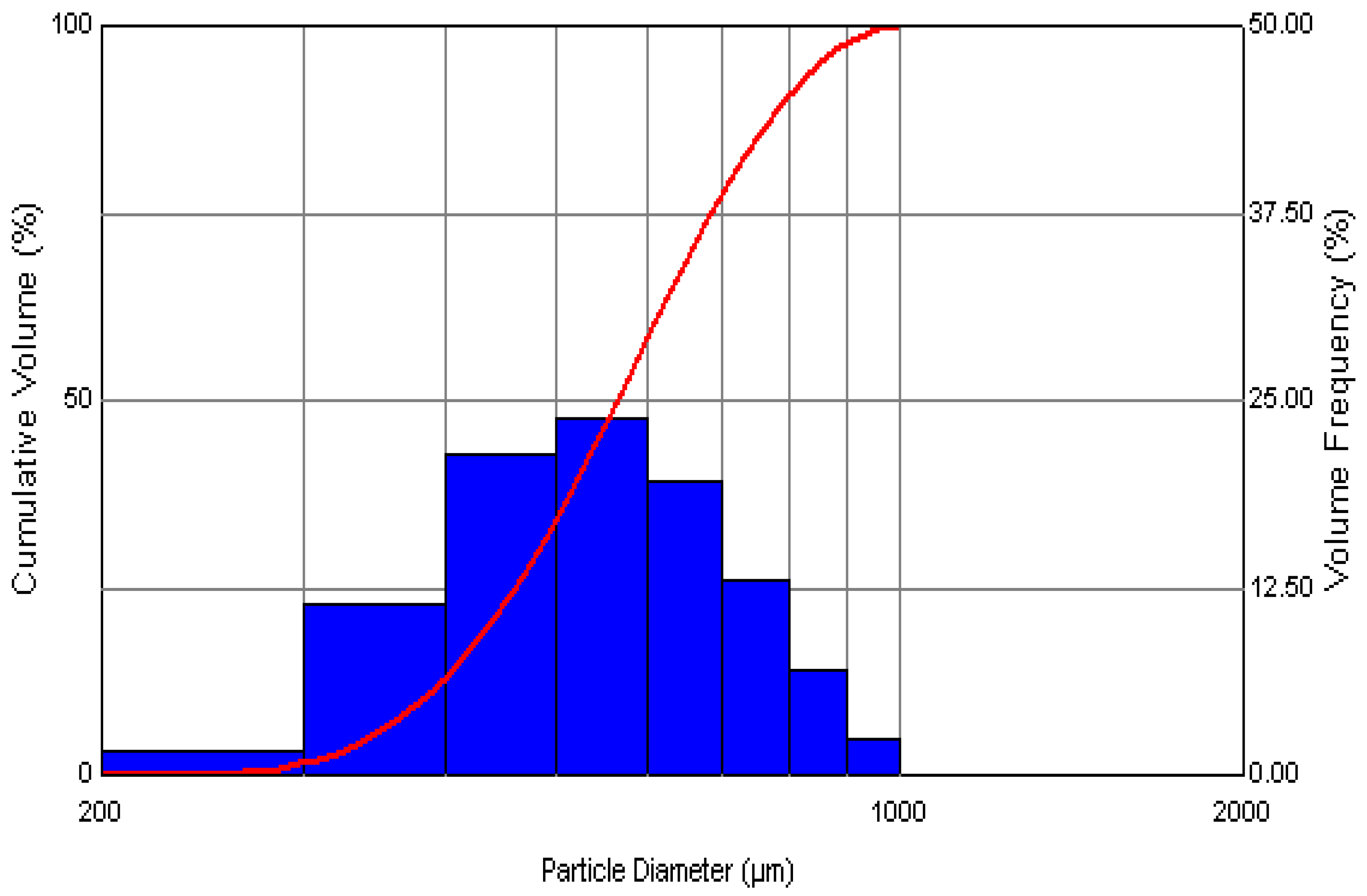
In particle sizing, and bubble sizing by extension, there are several methods to represent the BSD. In the work presented herein, there are quite a few larger bubbles in the steady flow condition compared to the oscillatory flow condition. However, with regard to the bigger bubbles, more are produced by the steady flow, with a significant contribution to the BSD due to the effect of the volume on the average sizes. The volume of a larger bubble has a much higher weighting than the smaller bubble on gas throughput. Therefore, a bubble of 1 mm size has a 1000 times greater impact in terms of volumetric flowrate than a 100 µm bubble. This means that a thousand 100 µm bubbles would need to be produced to have the same volume as that of a single 1 mm bubble resulting in a skewed BSD due to this. Consider 1000 bubbles each of diameters 1 µm, 100 µm, and 500 µm. Their number contribution is the same whereas their volume contribution is much higher, as shown in
Figure 4.
Number mean is important when only the number of bubbles/particles is of interest. This is used when the number of bubbles is more important than obtaining the size (for example, applications such as dispersed air flotation and froth flotation). Differences in bubble size based on number mean and volume contribution has been described in the literature [
58,
59].
Average bubble sizes vary with the particular data set being observed and are equally dependent on the analysis. However, this is amplified due to the change in the bubble dynamics. Analysis of single-bubble generation would not be a problem since both the average sizing values are fairly close to each other since the variance is lower. However, for cloud bubble dynamics, these effects become prominent. When it comes to over 1 × 10⁶–1 × 10⁹ bubbles, even with a narrower size distribution, large variances in bubble sizes are observed, depending on which method is used. For mass and heat transfer, it would generally be more appropriate to use void fraction for average bubble size for large sample sizes. The analysis utilises certain statistics (moments) used for calculating the different types of diameters.
The volume mean diameter is known as D
4,3, also known as the third moment. Similarly, the surface area mean diameter is known as D
3,2—the Sauter Mean Diameter [
30,
59,
60].
The Specific Surface Area is the total area of the particles divided by their total weight.
Percentiles have been commonly used in particle sizing that determine the portion of particles which lie below or above the said percentage.
Those used with particular emphasis are–Dx(10), Dx(50) and Dx(90).
These values are also used to calculate the span of a BSD, which is actually the width of the size distribution. This is done using
Percentiles become important in order to characterise the histogram and size distributions.
All of these values can be found in the British Standard BS2955:1993 or the ISO 13320:2009.
6. Hypothesis
The hypothesis of this paper is that acoustic methods are most accurate for small microbubbles since they are specific to bubbles, they do not miss small bubbles (since they rely upon the RBA) and can also be used in particle based systems due to this property (they neglect particles). They can also be used holistically rather than taking small sample sizes.
Microbubble size distributions cannot be visually determined but need careful measurement and analysis in order to better characterise the system.
The use of the fluidic oscillator as a means of controlled microbubble generation mediated by frequency changes aids in testing the hypothesis as it generates microbubbles of different size distributions at various frequencies. The crux of the hypothesis lies in the smaller population of the bubbles in order to test whether they ‘hide’ among the larger ones, which can be achieved using the fluidic oscillator. Whilst larger bubbles are simple to generate, smaller bubbles generated with a ceramic sparger are not as simple unless noncoalescent media [
61] or surfactants [
62,
63] are added, which affect the sizing and visualisation paradigms.
7. Methods and Materials
7.1. Sparger
Sintered alumina spargers (2 μm average pore size, 2 off–50 cm
2 area), which produces a cloud of fine bubbles approximately 500 µm in size under steady flow [
58] is used as the sparger in this study. This sparger, when coupled with the fluidic oscillator, can generate down to 7 μm in average bubble size (number average) [
58].
7.2. Fluidic Oscillator (FO)
A fluidic oscillator [
64] (FO) is coupled with the accompanying pneumatic setup, Malvern SprayTec, Acoustic Bubble Spectrometer (ABS), High Speed Visualisation Setup, and frequency analysis kit. The frequency of the oscillator determines the rate of bubble generation.
7.3. Frequency Measurement and Fast Fourier Transform
Impress G-1000 pressure transducers and ADXL335 accelerometers are used. Fast Fourier Transforms are workhorse algorithms in signal processing, converting a signal from one domain (time or space) and to the frequency domain (and the inverse). The associated power spectrum provides a facile estimate the frequency of the oscillatory flow from the fluidic oscillator. LabView was used to acquire the signal and process it.
7.4. Microbubble Generation Setup
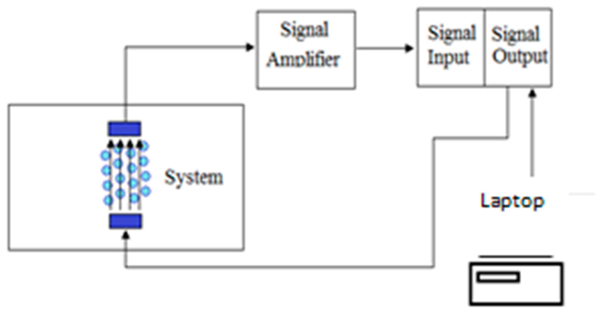
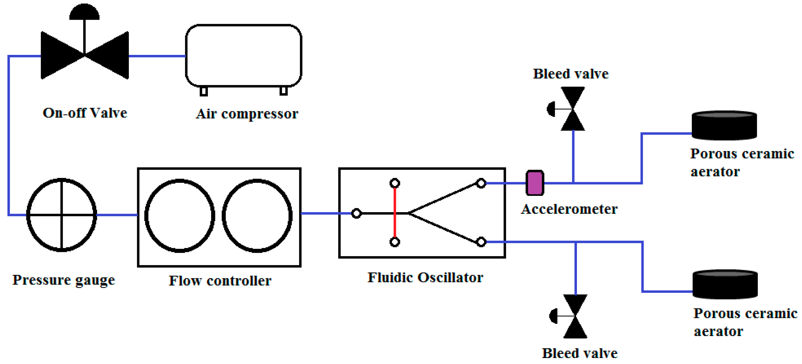
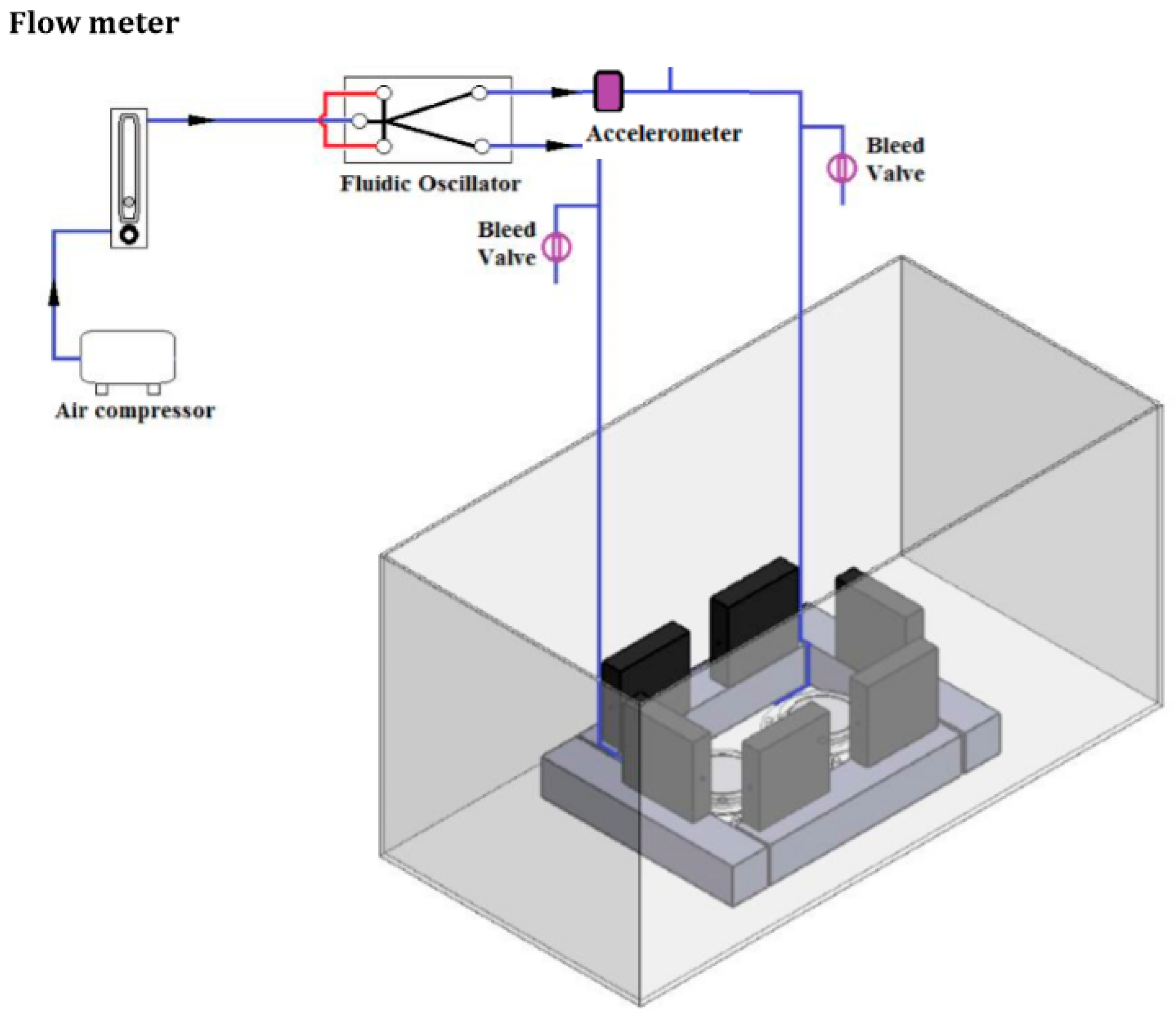
The global flow rate (see
Figure 5) is controlled by a flow meter while an accelerometer is placed at one of the legs in order to record the frequency of the FO for maintenance of experimental conditions. A relatively high global flow rate is required in order for the FO to oscillate, but the bleed valves control the flow rate that the spargers receive. Two configurations generating ten frequency conditions for bubble formation are used in the FO–sparger combination.
Twelve averages were taken for the ABS, with four each for the optical and photonic method. There is less than 3% error in the readings estimated for the ABS and SprayTec, while the optical method has 5% error levels.
Systemic conditions were kept as constant as possible whilst comparing the different characterisation methods in order to introduce the least amount of replication error as possible. Since each technique has their own drawbacks and advantages, slight variations to the actual methods were required. For example, photonic and optical (single camera systems) methods can only be used for a single plane to image accurately or in a small space, so extrapolations have to be made. The acoustic method can size the entire population, but the hydrophones require separate use for two equiresponsive diffusers. The equivalence of the double sparger/hydrophone system to a single sparger plume is the major replication assumption made.
7.5. Optical Methods–High-Speed Photography
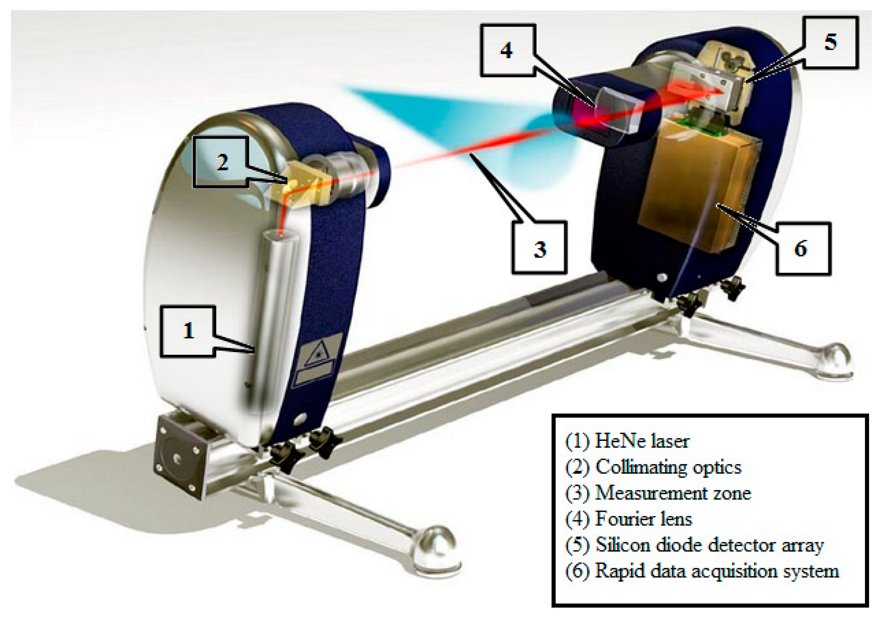
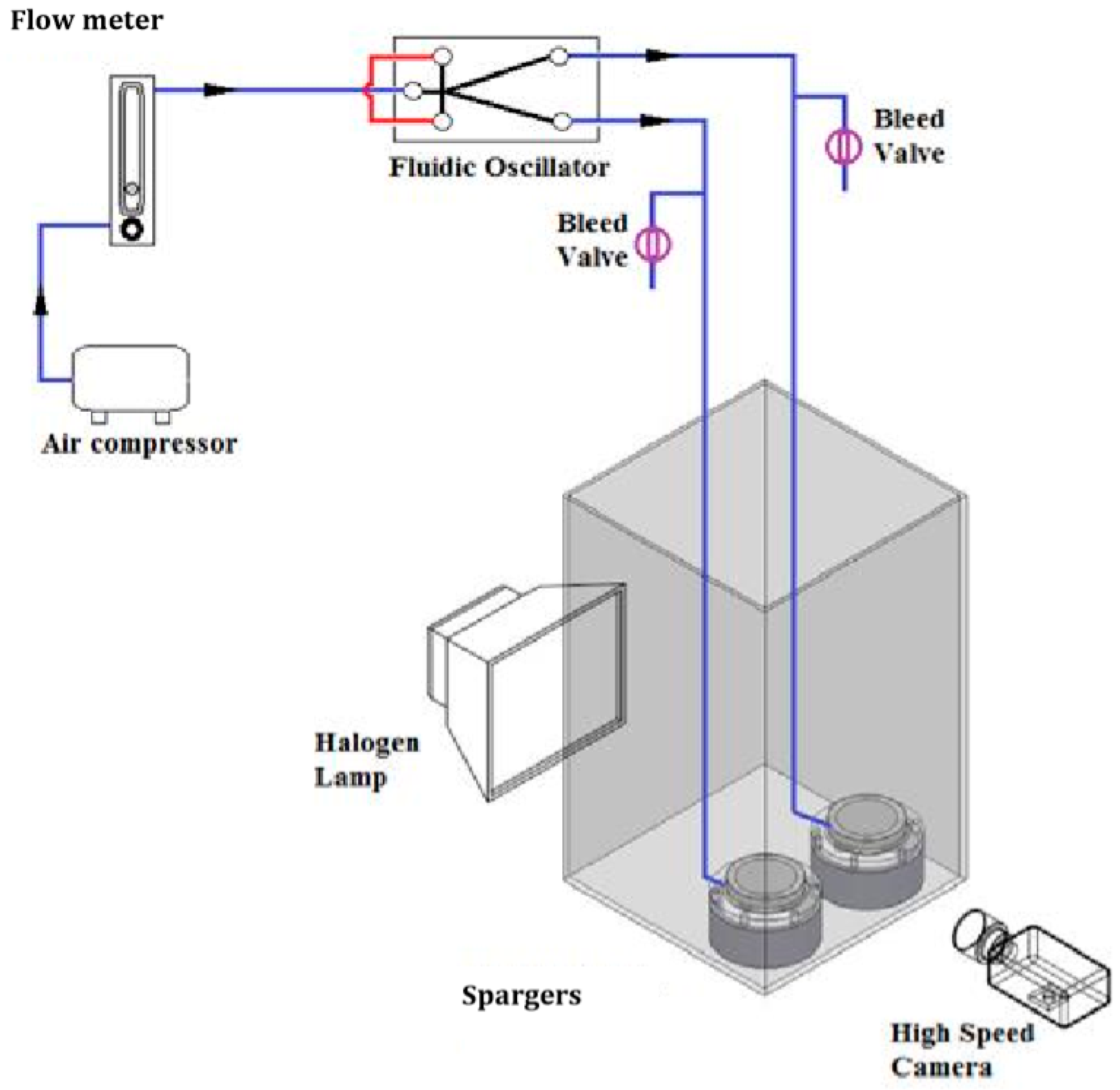
The visualisation device (see
Figure 6) is a high-speed camera, (Photron FastCam S3) capable of 250,000
fps with a resolution of 1024 × 1024 and provided with a lens (Nikon Nikkor Lens, 1.8 D). The region of interest used was 1.764 cm
3 (this takes into account the different focal planes used in order to capture sufficient data).
A single plane is used, as the image analysis software is not designed for a cloud of bubbles. Desai et al. [
58] is the only other significant work done on 3D cloud bubble dynamics, but no automated image analysis on a 3D bubble population has been developed yet except attempting to do so [
7]. It was assumed that it would be an equiresponsive surface and that a single plane could be representative as a microcosm of the overall cloud dynamical system. The appropriateness of this assumption in representativeness is one area where errors in measurement are introduced.
The systemic conditions are kept constant as described in the bubble generating system section.
7.6. Photonic Method–SprayTec
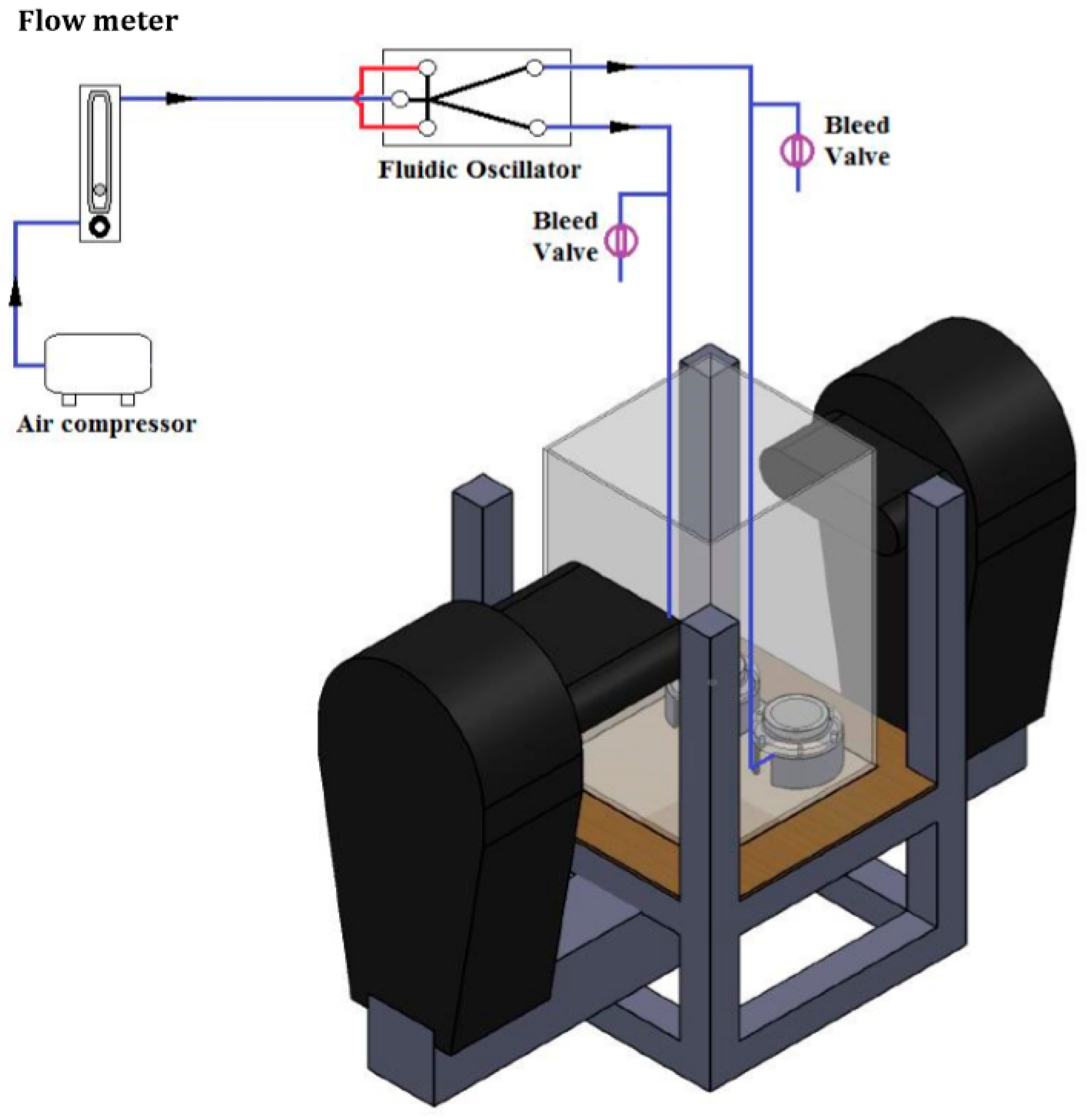
SprayTec (see
Figure 7) images a small sampling window. Within this field of vision, the statistical homogeneity and stationarity assumptions are made: bubbles are being produced equally from all regions of the spargers and that surface imperfections are negligible. The uniformity of this assumption is the same problem as observed for optical methods. The gamut of the bubble population is possible only for a small test cell in case of bubble generation. Usually it is not required when compared to a spray. The SprayTec is able to infer BSDs whilst automatically adjusting for the change in refractive index due to the addition of the test cell. For an example, see
Figure 8.
The 300 mm lens was used with particulate refractive index set at 1+0.01I, dispersant refractive index set at 1.33. The particle density was 1.23 g/cm3 with residual set at 2.15% for the data.
The transmission measurement involves a spatial filtering of the collimated laser beam pre and post transmission through the bubble cloud. The spatial filter is the pinhole at the centre of the detector array. As well as being used to ensure the detector array, it is centred on the laser beam and also rejects any scattered light. This is important, as it removes backscatter for most cases. However, for high scatterers, such as bubbles, due to concentration effects, multiple scattering inevitably causes some light to be rescattered back to a near-zero scattering angle. The laser used in SprayTec is a 632.8 nm, 2mW helium-neon laser. The transmitter contains the He:Ne laser source which produces a collimated beam of 10 mm diameter with a wavelength of 632.8 nm.
The detectors (over 30 of them), with the use of high-efficiency spatial filtering, means the concentration calculation is reliable over a much wider concentration range than a method based on measuring total scattered energy. This method requires no calibration and is able to carry out bubble sizing in real time. The media set are water and air.
7.7. Acoustic Method–Acoustic Bubble Spectrometer (ABS)
The measurements involving the ABS used four pairs of hydrophones with resonant frequencies at 50 kHz, 150 kHz, 250 kHz and 500 kHz. This ensured that the entire gamut of the BSD could be observed. The hydrophones were placed opposite each other and the bubbles insonated by ultrasound. The frequency of insonation determines bubble size and attenuation provides the number of bubbles. The bubble sizes obtained are for the entire sparger and are near real time measurements.
Figure 9 shows the setup for the experiment with the ABS.
8. Results
A comparison is made on the bubble sizing with the three methods. To ensure repeatability of bubble sizes, the frequencies of oscillation was measured using accelerometers and a pressure transducer.
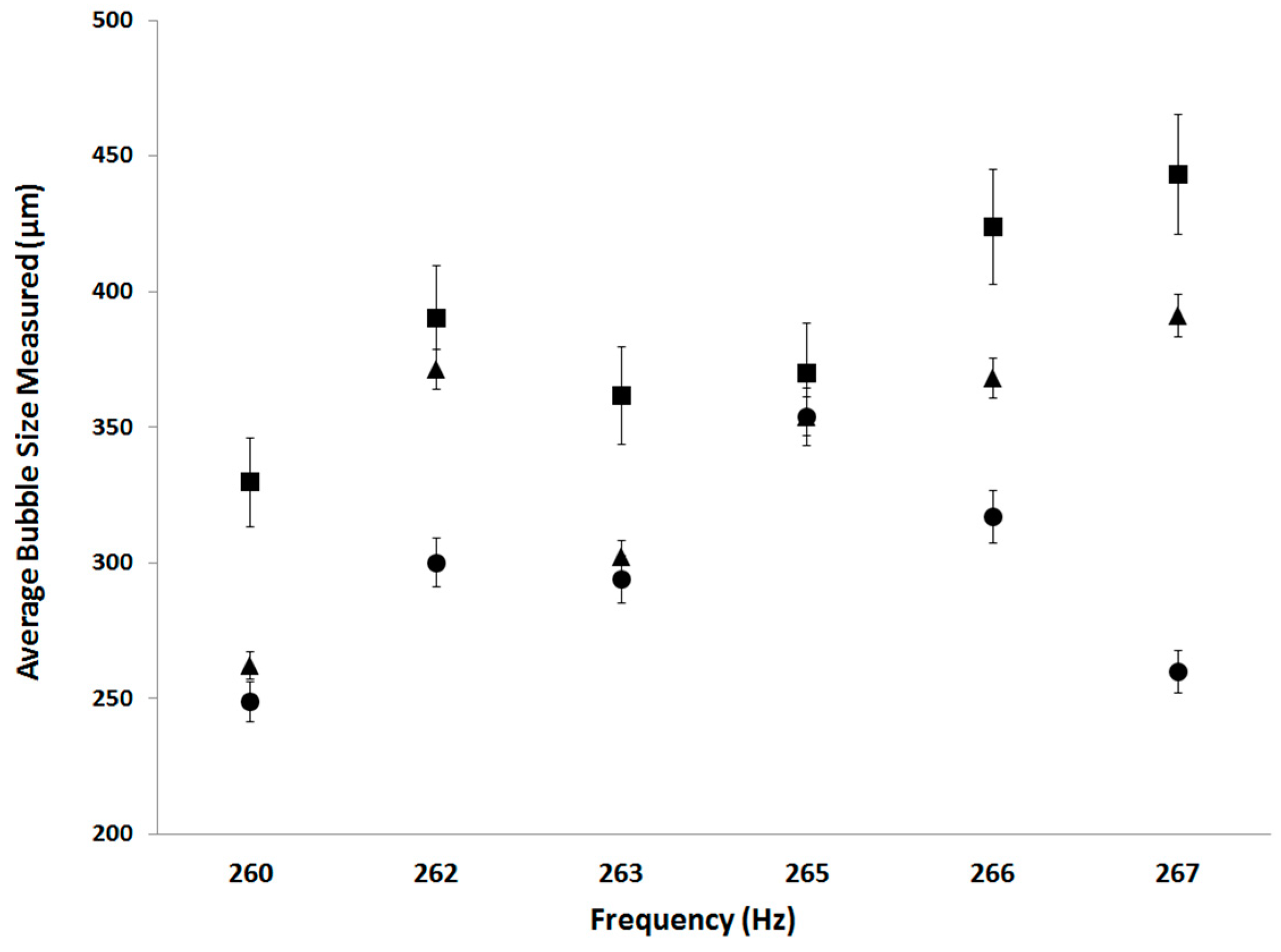
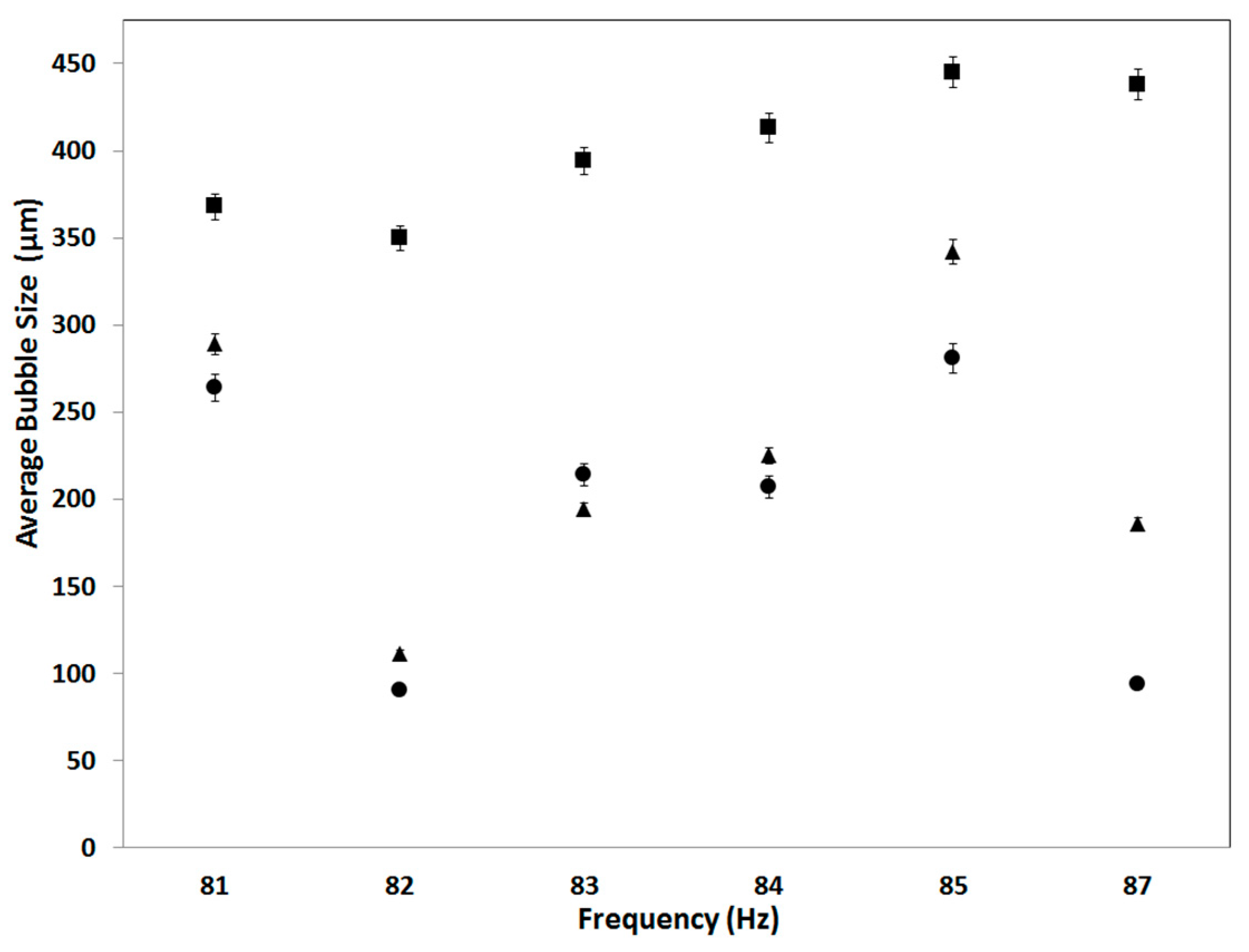
Figure 10 and
Figure 11 show the average bubble sizes estimated for the spargers at different FO frequencies at different configurations using the three visualisation methods.
The acoustic method shows an average bubble size with smaller bubbles than the other methods. Even for conditions with the same average bubble size, their respective BSD is different.
Although the SprayTec seems to correlate well with the high-speed camera and the ABS, the average bubble sizes obtained by the ABS are lower. Substantial data is condensed into a single point, resulting in a loss of fidelity and understanding. The window used for bubble sizing also influences the determination of the bubble size. For ABS, the sizes obtained can be smaller if using a smaller acquisition window. Due to the number average calculations, the average bubble sizes become much smaller.
The major point to note is the region of interest (ROI) recorded for these systems (Optical ROI–1.76 cm3, Photonic ROI–2 cm3, ABS ROI–353 cm3). Normalisation on ROI had to be carried out as the optical method has a single plane of interest which also depends on the focal plane. The photonic method depends on the ‘width’ of the laser (6 mm) and the depth of the spray. Since the light diffracts and the sensors record it, it is the beam of light for which the spread is measured. This means that the accuracy is reduced for a polydisperse distribution, but increased accuracy for a narrower size distribution. The averaging performed reduces the induced errors. The ABS records a much larger sample size, due to the volume subtended by the hydrophones being much larger. This results in a more comprehensive BSD.
9. Discussion
The results in
Figure 10 and
Figure 11 demonstrate that there is a certain size difference obtained for the various conditions. This is due to the loss in fidelity due to the reduction of an extremely large dataset into a singular point. Since bubble sizing normally deals with the number average, it is used here.
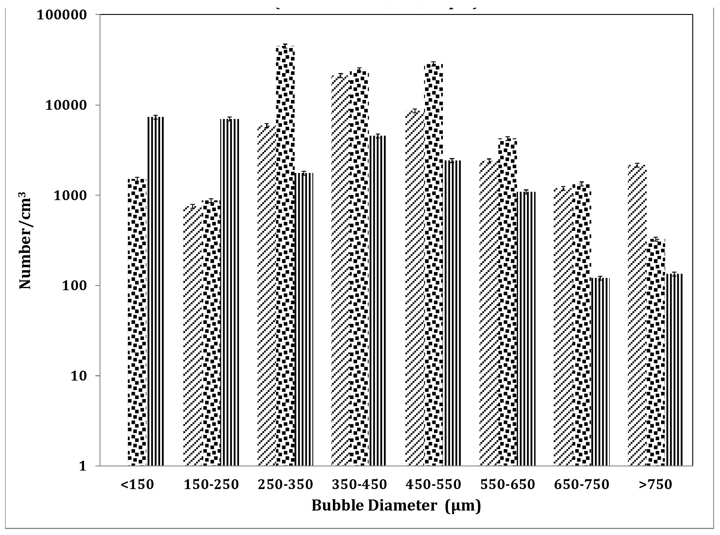
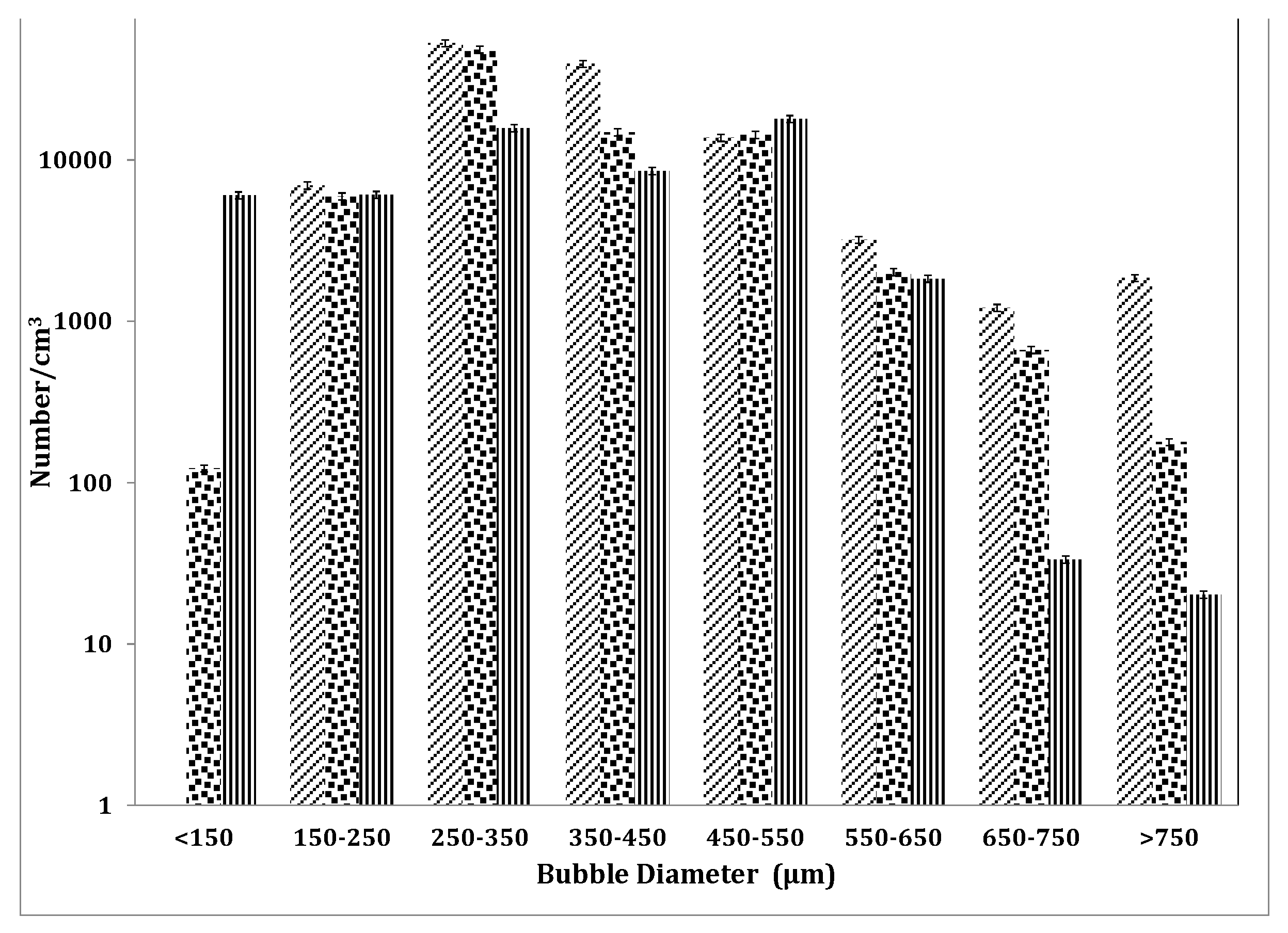
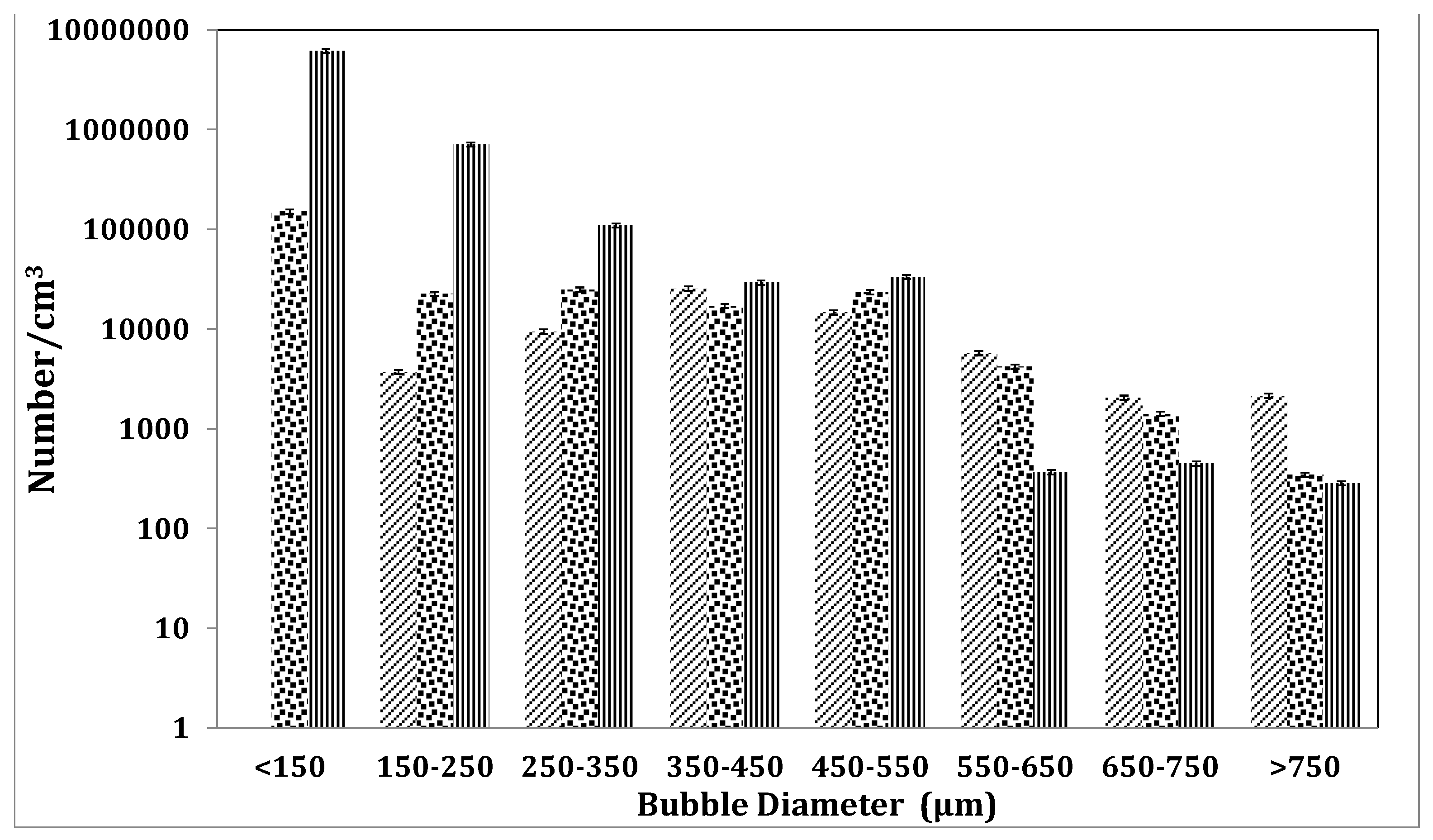
For
Figure 12, the bubbles formed are recorded over several averages for an acquisition time of 200 ms in order to collate the maximum breadth of information achievable with the available computational power. This is for a normalised volume of 1 cm
3 and the y-axis is a logarithmic scale. As can be seen, the bubbles smaller than 150 µm are recorded for both SprayTec and the ABS.
A general trend that was observed is that the average measured by ABS is smaller than the SprayTec or the high-speed camera. Several averages are taken for the SprayTec automatically, which enhances accuracy, especially for narrow size distributions. High-speed photography and the SprayTec cannot differentiate between bubbles and particles whereas the ABS measures only bubble size. ABS also obtains the gamut of the bubble size within the volume of liquid between the two hydrophones. However, this also means that one has to use larger bins, shorter acquisition times and high-speed acquisition, i.e., a powerful computing package.
Figure 13 is an example of a BSD expanded from a single point from
Figure 11. The differences in the bubble sizes for the three methods can be seen here. Whilst the average bubble size might be similar, the BSD is quite different.
Figure 12 is a BSD expanded from another point from
Figure 10. However, it can be clearly seen that the BSDs are different and just merely balanced out even with the averaging performed. The ABS and SprayTec measure the smaller bubbles and these bubbles are not accounted for by the optical methods. There are also larger bubbles observed but the per cm
3 figure is a construct in some sense for the SprayTec and the optical method. This is because optical methods measure a plane and not a significant depth. The depth has to be introduced artificially and expanded. Likewise, for the SprayTec the volume has to be modified appropriately in order to get values per cm
3. The ABS on the other hand, has to be reduced by calculations as the gamut and volume captured is larger than 1 cm
3. This brings about a more statistically significant value but has the drawback that salient features can sometimes be missed due to lack of computing power. The BSD would be better for the SprayTec if the sampling chamber were designed accordingly so as to be able to collate a comprehensive size distribution.
The ABS needs to have the sampling chamber big enough for the hydrophones to fit in, in order to obtain a BSD. With this in place, the ABS can also be used outside the liquid and in another liquid if the acoustic impedance is matched. This means that the ABS can be used in optically opaque media. Liquids usually have a higher acoustic transparency over optical transparency. If the acoustic impedance of the liquid is known, and the resonant frequency of the hydrophone can be obtained, ABS can be used for the bubble sizing in a variety of liquids. This is not true for optical methods nor for photonic methods.
Photonic methods depend on diffraction and therefore are not specific to bubbles. The ABS is bubble specific, while optical methods tend to miss this distinction and also have problems with non-circular or overlapping bubbles. Bubbles with neighbouring particles affect the BSD obtained with SprayTec, while image analysis is made difficult for overlapping or coalescing bubbles. Scattering of laser light is very sensitive to changes in any inherent conditions (temperature, contamination, smaller bubbles, smudges, etc.), resulting in errors in measurement. Scattering also neglects smaller bubbles as they ‘hide’ behind the larger bubbles. Both SprayTec and the ABS depend on inversions as well as statistical techniques in order to infer a BSD. Inversion propagates errors in the measurement to errors in the estimated BSD.
The ceramic spargers are commercially available microbubble generators and are supposed to be equiresponsive. This is also an assumption that introduces errors in the system as not only does this create an error for the three methods but can also introduce errors with the ABS since it treats bubble clouds from two spargers at the same time. Smaller bubble sizes might be observed using acoustic methods since liquids are more transparent to sound than light. The bubbles are two phase entities with distinct boundaries, possibly able to scatter light in such a way that the entire population is not measured. As demonstrated previously, acoustic methods are more consistent for bubble sizing with the ability to provide a wider range BSD.
In case of optical and photonic techniques, vignetting might affect the results due to the incorrect measurement of light scattering angles resulting from incorrect focusing. This is easier to correct for optical methods but not so with photonic methods. Optical methods also suffer from the fact that the lenses and focusing ability can very limited. The bubble size can be either magnified and a small ROI can be used, otherwise a broader region but a larger ROI is used. This means that sub-150 µm measurements would result in a substantial redaction for bubbles being measured.
A point from
Figure 11 is expanded into a BSD in
Figure 14. The ABS consistently measures smaller bubbles resulting in a smaller BSD and much larger number of bubbles, which would be severely skewed for the other two methods due to the problems of ‘hidden’ bubbles and overlapping bubbles. These, however, are not missed by the ABS. Thus, the obtained BSDs vary considerably. When volume averages are taken, smaller bubbles do not contribute as much as the larger bubbles. However, the problem with this measurement is that whilst it will reconcile the data obtained for the acoustic method and SprayTec more successfully, it shows much larger average bubble size for the optical method, since then the volume contributions become much larger. Just as a billion 1 µm bubbles occupy the same volume as a single 1 mm bubble, the bubbles >750 µm will have a larger contribution. This will result in a much larger average bubble size for the optical method. The D50 and D
4,3 are also, therefore, not that useful for this exchange. This also removes the effect that the small bubbles have on the BSD. The smaller bubbles have a much higher impact on transport phenomena due to their high internal convection/mixing as well as the rate of transfer [
65]. This means that with singular values in bubble sizes, one can have similar values for the system but highly varied performances that are not effectively described. Since the transport phenomena associated is highly dependent on the size of the bubbles in question, the composition of the bubble cloud can make a large difference.
10. Conclusions
Each of these methods offers distinct drawbacks and advantages.
SprayTec and the ABS are indirect methods used for inferring BSD but offer near real time results with enormous acquisition capabilities. High-speed photography/videography are a direct method but are not as effective for bubble cloud dynamics, requiring post processing and image analysis.
The SprayTec needs an appropriately sized chamber for sampling to engender the gamut of the bubble spectra and is better for a smaller sample whereas the ABS is better for a larger system. The ABS operates more effectively when the hydrophones are placed in the liquid medium whereas the lasers need to have a clear path to traverse through.
The ABS does not require a sampling chamber to be transparent whereas SprayTec and high-speed photography have this prerequisite. An acoustically transparent substance need not be an optically transparent one.
Therefore, application-specific constraints will dictate which system ought to be used.
Bubble sizes obtained are smaller when the ABS is used because the gamut of the bubble spectra is obtained for this system whereas SprayTec can only observe a small section. A plane had to be used for the high-speed photography due to complications relating to the overlapping bubbles as well as image analysis for cloud bubble dynamics.
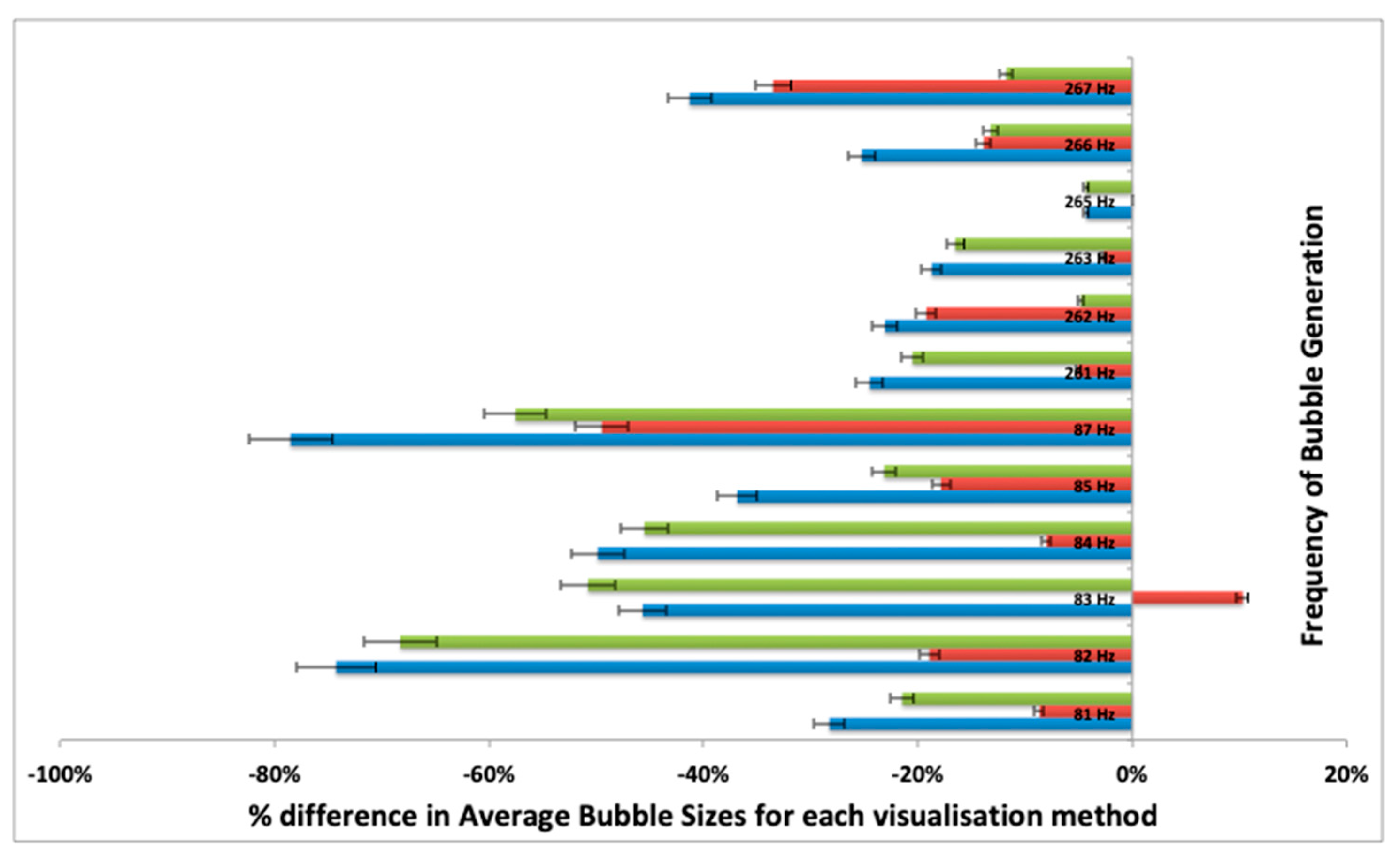
Figure 15 shows the percentage differences between pairs of methods among the three different visualisation techniques. It is observed that, as per the hypothesis, there is a wide difference with the ABS-Optical (79%) and SprayTec-Optical (68%)-based systems. There is closer agreement with the ABS and SprayTec due to the controlled conditions in this experimental setup (nearly zero particulates/additives/contamination in the test water) and the reasons discussed previously agree with the close alignment with the results. One point, there is a large discrepancy between the SprayTec and ABS (49%, as per
Figure 14) at 87 Hz condition, and the hypothesis being tested. Smaller bubbles are hidden from the SprayTec and Optical type systems, but not for the ABS–is seen herein. Similarly, the 257-Hz point shows nearly 38% discrepancy between SprayTec and ABS, which can be observed in the BSD (as seen in
Figure 12), where the smaller bubbles were not being recorded for the SprayTec. When the bubble throughput is low, the differences between the SprayTec and ABS are reduced significantly, and the averaging results in equal average bubble size, even though there is a difference in the BSD (as seen in
Figure 13). It seems likely that the cause of the discrepancy between the two techniques at high bubble throughput is as a result of bubble–bubble interactions and that if it is not possible to measure at low bubble throughputs then modifications to Mie theory being implemented into the analysis may result in a more robust analysis.
Depending on the uses, availability, expertise and the application, different methods can be used to compute the BSD and upon significant inference, accurate BSDs can be estimated.

 ,
, 


 -ABS,
-ABS,  -SprayTec,
  -optical methods ).


 -Optical method,
  -SprayTec,
  -Acoustic bubble spectrometry.


 -(Spraytec- Optical),
  -(ABS- SprayTec),
  -(ABS-Optical)).
