1. Introduction
The process of wetting of a solid substrate by a liquid is of paramount importance in several industrial processes [
1]. When this is driven by external forces, it is customarily called forced wetting. Forced wetting by a confined liquid—for example, by a droplet—is also termed spreading, when only one edge of the droplet moves, or sliding, when the droplet altogether (both edges) moves. In case of dynamic (non quasi-static) spreading and sliding, hydrodynamics have an essential role and literature on the subject is especially vast. This is because there is no fundamentally exact mesoscopic mathematical description of the problem, and thus several approximate techniques have been developed [
2,
3,
4]. The situation is relatively simpler in the case of quasi-static spreading. The criterion for quasi-static spreading to occur is the characteristic time of force variation being much smaller than the characteristic time of droplet motion. In this case, the shape of the droplet is completely determined by force (or energy) balances. This shape can be easily determined by the well-known Young–Laplace equation. Even in complex cases considering disjoining pressure [
5], substrate elasticity [
6], and surface roughness [
7], the Young–Laplace equation is valid far from the contact line, and the additional complexity can be dealt with by using an effective contact angle instead of the real angle. However, the motion of the contact line, even during quasi-static spreading, is an unresolved issue. In the two-dimensional case, the corresponding problem is somewhat trivial, as the contact line moves when the contact angle exceeds the advancing contact angle value φ
A [
8]. In three dimensions, however, a whole distribution of contact angles may exist. The contact line moves when the maximum angle exceeds φ
A. This occurs not only at a single point, but with a whole portion of the contact line moving. Thus, a model for the motion of the contact line is needed.
A very elaborated (albeit phenomenological in nature) model based on energy minimization of the droplet was proposed a few years prior to this study [
9] and has been employed by several authors [
10,
11]. The surface evolver open code was used to initially find the contact angle distribution and then the contact line was moved in a way that the moving distance at each point was proportional to a function that included the local contact angle and advancing (or receding φ
R) contact angle. The whole procedure was iterated until the contact angle profile exceeded φ
A in no location. This approach led to rather questionable results, as large areas of the contact line with contact angles equal to φ
A or φ
R appeared according to results presented in [
9]. A different approach, again using surface evolver, was proposed in [
12]. The contact line in this model evolved in a way that the contact angle distribution followed a specific functional form proposed in [
13].
From the above discussion, it becomes clear that the contact angle distribution knowledge is essential for the development of contact line motion. Several attempts to suggest contact angle profile shapes based on numerical analysis led to controversial results [
14,
15]. What is considered the best contact angle profile is the generalized third order polynomial function (with respect to the azimuthal angle) proposed in [
13]. This was derived on the basis of numerous experiments using a rotating camera. However (although some shape corrections have been made in the techniques) it has not been possible to observe contact angle from an arbitrary point of view. As a virtual experiment to prove this, imagine a square contact line. The camera will observe the same fictitious contact angle from several angles of observation. Further from the contact angle profile, a complete model of the contact line evolution during application of a tangential force to a droplet was proposed in [
13], based exclusively on experimental data. According to this model, the contact line is elliptical, with an ellipsis aspect ratio being a specific function of the tangential Bond number, Bo
T. Another function of Bo
T was proposed for the ratio of minimum to maximum contact angle during spreading. These functions are independent from droplet volume.
As it is discussed above, the direct experimental identification of contact angle distribution is a very difficult task. On the other hand, identification of the experimental contact line is a very easy process for omniphilic surfaces (only a top image of the droplet is needed). Thus, a large number of experimental data on contact line motion during spreading under several applied force sequences is necessary in order to develop a model for contact line motion. This idea is supported in several ways in the present work. It is stressed that the focus of the present work is not to develop techniques for the solution of the Young–Laplace equation. The proposed techniques are instead used as a vehicle to demonstrate how the experimental results on contact line shape evolution can be handled to produce data for the development of contact line motion theories.
The structure of the present work is the following: First several results for the contact angle distribution as predicted by the non-linear Young–Laplace equation for circular and elliptical contact lines are presented. On the basis of these results, it is shown that ellipsis is not an acceptable shape for the contact line under tangential force. A contradiction with the model of [
13] thus appears. Then, a simple semianalytical technique for the linearized Young–Laplace equation is developed and applied for the contact line evolution under a tangential force assuming a specific contact line shape that has been observed experimentally. The results are extensively discussed, and the direction of the required experimental studies on the subject is shown.
2. Problem Formulation, Results, and Discussion
It is noted that any shape of the droplet contact line is admissible as far as the contact line profile includes values between φA and φR. This is why a contact line motion model is needed—to choose the real one from the admissible shapes as the contact line evolves. A contact line shape can be achieved by way of droplet deposition on the substrate and/or by applied force sequences. An alternative situation is one of pinning, in which the contact line shape is determined by the structure of the substrate (e.g., an adverse step). In this case, the advancing contact angle can be (effectively) exceeded with no contact line motion.
The governing equation that determines the shape of the droplet is the so called Young–Laplace equation. This equation is a statement of total droplet energy minimization. In particular, the energy contributions that depend on droplet shape are the surface energy and the potential energy associated with body forces. The relative contribution of the two types of energy (potential/surface) are expressed through the dimensionless parameter called the Bond number. In the case of omniphilic surfaces, the Monge representation of the droplet surface in Cartesian coordinates can be employed [
16]. This leads to a much simpler mathematical problem than the spherical coordinate representation, which has the advantage of applicability even for contact angles larger than 90° [
17]. If the Cartesian coordinates are denoted by x, y, and z and the droplet shape is denoted by z = f(x,y) the governing equation (in its dimensionless form) for the droplet shape takes the form
where the variables x, y, z, and f are normalized by a characteristic length L. The two Bond numbers (normal Bo
N and tangential Bo
T) are computed as ραL
2/σ, where ρ and σ are the density and the surface tension of the liquid and α is the corresponding (normal or tangential) acceleration field value. The case of a prescribed droplet basis contour will be treated first. In this case the boundary condition for the solution of the above equation is
Equation (1) is defined in the domain C that is included in the curve F(x,y) = 0, which is the functional representation of the contact line.
The parameter G must be derived from the requirement of the prescribed dimensionless liquid volume V (the nondimensionalization is made using L
3):
The above mathematical problem is solved numerically as follows: At first, Equation (1) is discretized using quadratic triangular unstructured elements. The resulting system of non-linear algebraic equations is solved through the Newton–Raphson procedure (internal loop). An external Newton–Raphson loop is also employed in order to find the value of G that leads to the required droplet volume. The choice of L is typically based on a characteristic dimension of the droplet basis contour. Indicative results for three basis contours will be presented here.
(1) Circular basis. In this case, the circle radius is taken as characteristic length (i.e., L = R) and F(x,y) = x
2 + y
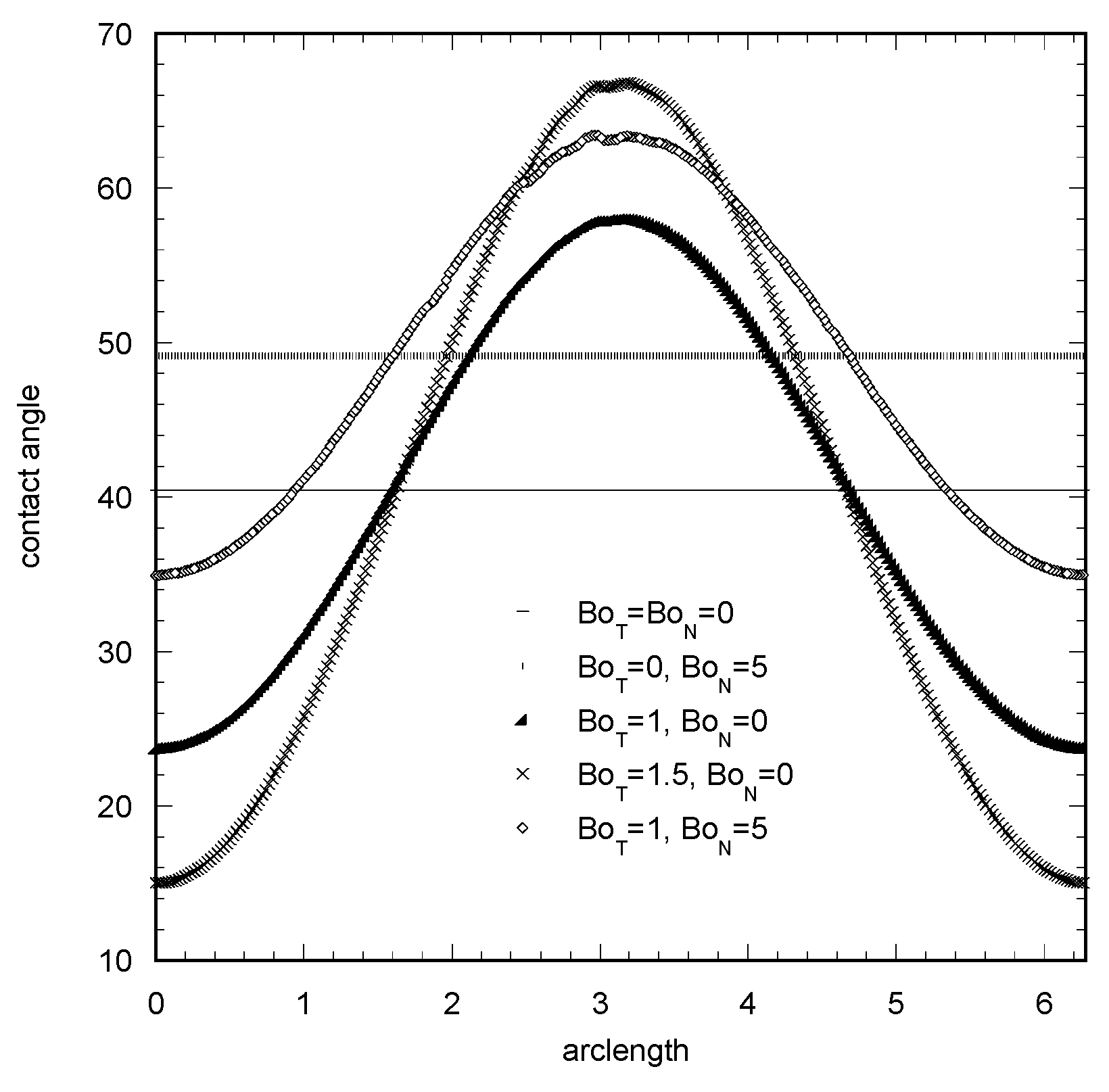
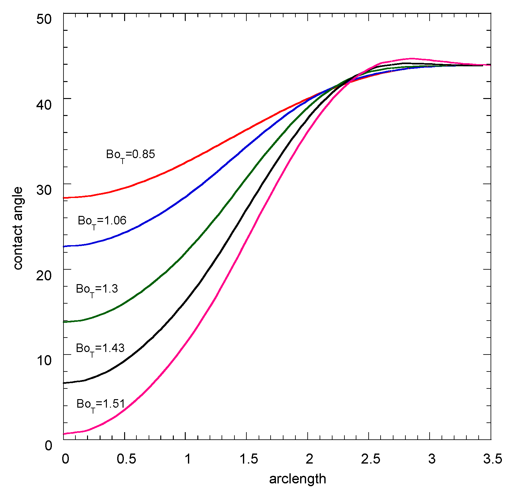
2−1. The Young–Laplace equation is solved numerically and the distribution of the contact angle along the contact line is computed by numerical differentiation. This problem has been extensively studied in the past, yet not in this particular context. The usual approach is to present the contact angle distribution with respect to the so-called azimuthal angle but, instead, we found it more fruitful to use the contact line length starting from the rear edge of the droplet for this purpose. The contact angle profiles for a droplet with a circular basis, dimensionless volume 0.6, and several combinations of applied tangential and normal forces are shown in
Figure 1. In the case of zero tangential force, the contact angle has a constant value (axisymmetric droplet shape). This constant value increases as the normal force increases and the droplet is squeezed to the surface. In the presence of tangential force the angle profile takes a unimodal shape with minimum at the rear edge and maximum at the front edge of the droplet. The difference between maximum and minimum angles increases as tangential force increases and decreases as normal force increases. In the limit of small contact angles (implying small slopes of the gas-liquid interface) the governing Young–Laplace equation can be linearized and solved analytically. The solution procedure is shown in
Appendix A for clarity of presentation. The final result for the interface slope distribution along the contact line is
where
is the length along the contact line, as defined previously, and I
o, I
1 are the modified Bessel functions of first kind with order zero and one, respectively. In terms of contact angle φ and azimuthal angle θ, the above equation can be written in a generalized way as
where A and B are functions of the normal Bond number. The above form qualitatively describes the effect of the parameters Bo
N, Bo
T, and V on the contact angle profile. This description is quantitatively accurate for contact angles less than 20°. An attempt is made to fit the contact angle distribution in
Figure 1 by Equation (5). The fitted distribution is similar to the actual one but with a somewhat larger spread. This means that the actual distribution can be represented well with a three-term Fourier series expansion (instead of a single term expansion of Equation (5)). The two additional terms accommodate the effect of non-linearity of the governing equations. As the contact angle increases, the number of required Fourier terms for contact profile representation also increases.
(2) Generalized elliptical basis. This implies an elliptical shape with a high aspect ratio resulting, for example, by pinning the droplet to the surface during deposition (the deformation is too large to be achieved by applied forces). In this case, the average half length of the two axes of the droplet basis is taken as characteristic length. The function F is given now as F(x,y) = (x/b)
2 + (y/a)
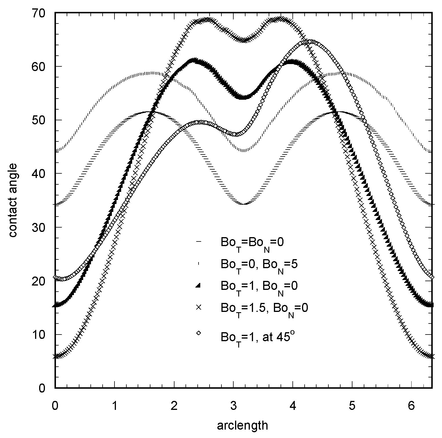
2 −1, where b, a, are the large and the small axis of the ellipsis, respectively. The contact angle profiles for a droplet with V = 0.6, a = 0.8, b = 1.2, and for several combinations of applied forces is shown in
Figure 2. In the absence of tangential force, the angle profile is bimodal with the two maximum positions at the side edges of the droplet, and the two minimum positions at the rear and front edges. The increase of the normal force leads simply to a shift of the profile to larger angle values. On the other hand, by increasing the tangential force, the locations of the maximum angle are transferred towards the front section of the droplet. In parallel, the difference between the maximum and the global minimum angle increases whereas the difference between maximum and local minimum decreases. The contact angle profile for tangential force applied to a direction of 45 °C with respect to ellipsis axis is also presented for comparison purposes. The profile is still bimodal, but it loses its symmetry with respect to droplet midplane along the large axis.
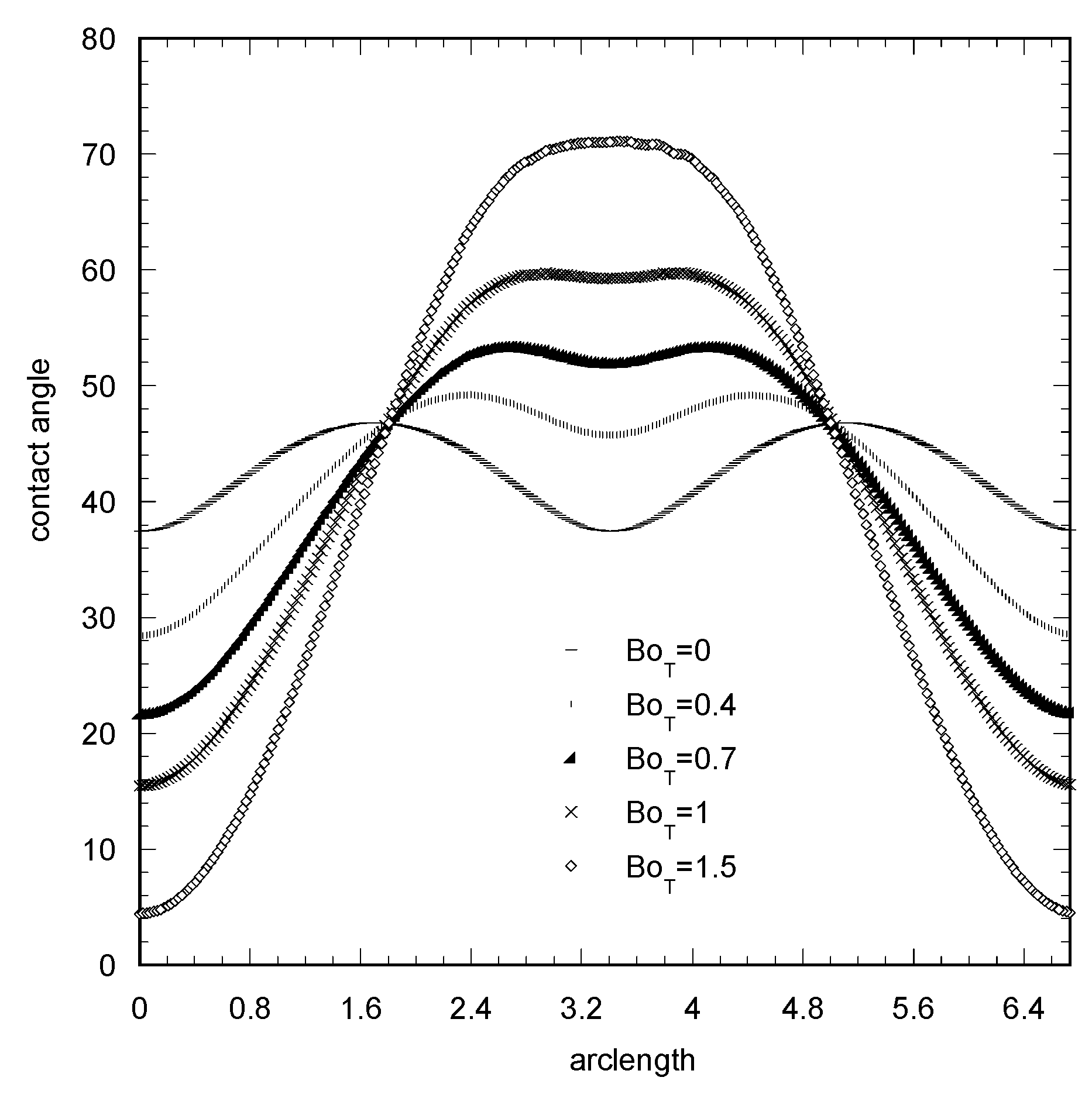
(3) Elliptical basis arising from tangential force to the drop. In this case, we assume an elliptical basis which is not due to deposition pinning but due to applied tangential force. An elliptical shape typical for this case (e.g., see [
13,
18]) with a = 0.96 and b = 1.2 is considered. An attempt to directly compare with the results of [
13] failed, since it is not possible to identify what is used as an equivalent drop diameter in the definition of Bond number in [
13]. Thus, an arbitrary characteristic length is considered for the purpose of analyzing the resulting contact angle profiles. These profiles in a case of zero normal force and for increasing tangential force are shown in
Figure 3.
In the case of small Bo
T, the angle profile is again bimodal, but as Bo
T increases it flattens at the front edge and at some force value the contact angle profile becomes unimodal. Hence, under the proper combination of contact line deformation and magnitude of Bo
T, the elliptical shape could be a possibility for the contact line, as it leads to a unimodal contact angle profile. Let us further examine this possibility by invoking the analysis in [
13]. According to that analysis, the Bo
T (as defined in [
13]) corresponding to the present aspect ratio (b/a = 1.25) is Bo
T = 2.6 (see Figure 12 of [
13]). The ratio between the minimum and maximum angles of the contact angle profile should be 0.62 (see Equation (16) and Figure 9 of [
13]). This value clearly corresponds to the bimodal profiles of
Figure 3. The acceptable unimodal profile has a much smaller value of this ratio. The correlations of [
13] are supposed to hold for any droplet volume; thus, the counter example presented here is enough to put it under question. The conclusion is that the contact angle profile shape and the contact line shape, both proposed in [
13], and the Young–Laplace equation are not consistent with each other.
Therefore, it appears that the elliptical shape is not the answer to the question of how the droplet contact line shape evolves during spreading induced by a tangential force. According to [
13], which refers to older literature, a combination of two ellipses with different large axes and common small axes leads to a much better description of experimental contact lines. More recent extensive experimental results reveal that the above description can be further simplified to a circle for the front (towards the applied force direction) and an ellipsis for the rear (opposite to the applied force direction) parts of the contact line [
19,
20,
21]. This means that if the circle radius is utilized as characteristic length, the shape of the contact line can be fully parameterized using a single parameter, b, which is the fractional elongation of the front part of the droplet (i.e., ellipsis large semiaxis/circle radius—1). In the present work, an approximate mathematical technique is developed for a closed form representation of the droplet shape. The method is restricted to the linearized Young–Laplace equation (small contact angles) and to the absence of normal force. This is a practically significant case, given that for small contact angles there may be considerable spreading, and the normal force has no large effect for slender drops so it can be safely ignored. In addition, a simple technique for the transformation of contact line shape to contact angle distribution is especially welcome in case of small angles, as in this case the direct angle measurement is very difficult and the sensitivity of the shape to the angle is very high. It must be reminded that for small angles the most reliable experimental contact angle measurements are based on the identification of contact line location [
22,
23].
The proposed method is based on the general approach of boundary weighted residual methods [
24]. These methods are based on enforcing a function, which is a solution to the governing equation, to confront the boundary condition. They have been used for the solution of the Stokes (biharmonic) equation for creeping flow [
25], Laplace equation for heat conduction [
26], and Poisson–Boltzmann equation for electrical double layer calculation [
27]. In all cases, some kind of an undulated surface preventing the completely analytical solution to the problem is involved. The method has no solid theoretical support and the domain of convergence is where the shape of the involved surface does not deviate much from the generating surfaces of the coordinate system used for the analytical solution of the governing equation [
28]. Thus, the method has been of rather small value and significance in the literature. However, in the present case, the shape of the contact line is never too different from that of a circle (corresponding to a polar coordinate solution) before sliding occurs, and this offers a good opportunity to the particular method as an effective practical tool.
The solution method is described in detail in
Appendix B. For an arbitrary shape of the contact line, a system of linear equations is solved for some coefficients and then the droplet’s shape can be written in terms of elementary functions. Let us study the convergence of the method compared with the largest index of expansion terms N for the particular contact angle shape of interest here. This can be written in polar coordinates and in terms of parameter b as
The application of the method shown in
Appendix B for the above profile with b = 0.5 (very distorted contact line) and for Bo
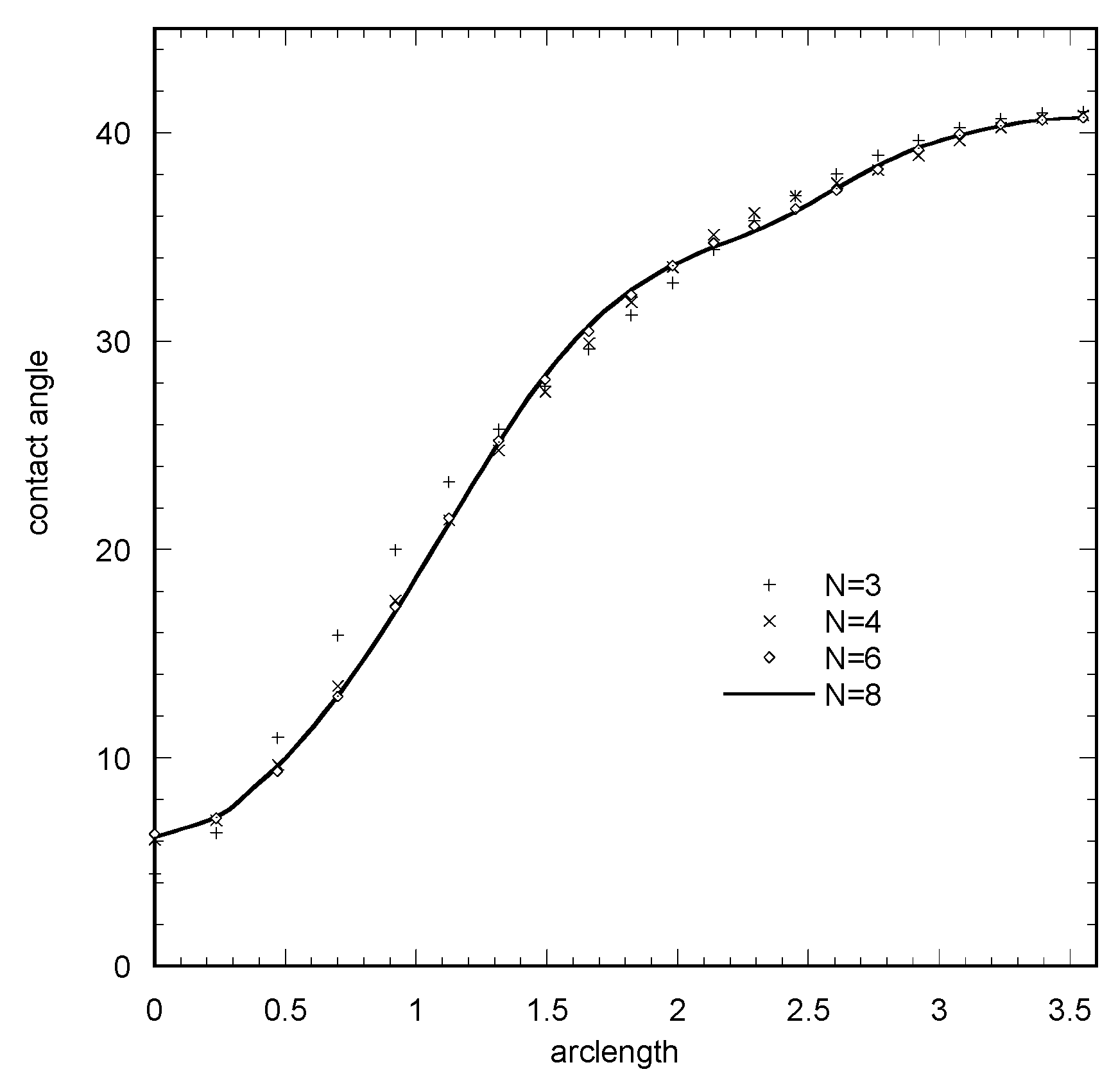
T = −1 and V = 0.6 for increasing values of N leads to the distribution of the contact angle along the contact line, as shown in
Figure 4. The negative tangential bond number means that the tangential force is applied to the opposite direction than the one having created the distortion of the contact line. The convergence study is presented for a negative Bond number because it corresponds to more stringent conditions. It is evident that complete convergence has been achieved at N = 6. Furthermore, to the convergence analysis, the resulting angle distribution is compared to the one resulting from the finite element solution with a fine grid, and coincidence is found.
Figure 4 suggests that even for N = 4, an accepted angle distribution can be derived. It is noted that the above situation holds for a relatively distorted contact line with b = 0.5. The required number N for convergence decreases as b decreases. Another issue is that the convergence test is performed against the contact angle, which is a measure based on the derivative of the droplet shape. Such a convergence test is stringent. A convergence test against the droplet shape itself leads to the very interesting result, in that in any case the expansion with N = 3 terms describes accurately the shape of the droplet. For comparison purposes, the number of unknown variables in the finite element technique is several hundreds and in surface evolver is several thousands. The important advantage of the proposed technique is that it offers a simple closed form representation of the droplet shape. This information can be utilized (i) for the reconstruction of the droplet shape from experimental limited image information and (ii) for the derivation of low-order weighted residual methods for the solution of the non-linear Young–Laplace equation. It is noted that the above discussion holds for homogeneous surfaces (at the scale of the contact line, i.e., a scale higher than the microscale). Localized heterogeneities in this scale can create high frequency perturbations to the contact line profile and dramatically increase the number of terms in the eigenfunction expansion needed for the contact line description. In this way, the stability of the solution technique is adversely affected.
The proposed approach will be used here to derive the contact angle distribution evolution as the tangential force increases. A droplet with V = 0.6 in the absence of forces is considered at the beginning. The droplet shape is spherical cap and the contact angle is uniform with φ = 36°. Then, the tangential force starts to increase. The contact angle is a function of the position along the contact line with the maximum towards the force direction and the minimum at the opposite direction. This profile has a simple cosine shape and continues to evolve up to the point that the maximum angle reaches the advancing contact angle φ
A (φ
A = 44° is assumed here). Then, spreading begins and the contact line shape becomes a function of the tangential force Bo
T. This shape is completely parameterized through Equation (6), and the evolution problem is transformed to seeking of the b value that leads, through the procedure described in
Appendix B, to a maximum contact angle equal to φ
A. For each value of Bo
T, the Newton–Raphson method is used to find b. In this way, the evolution of contact angle distribution is computed up to the case of the minimum angle being equal to the receding angle φ
R where sliding begins. The computed angle distributions along the contact line are presented in
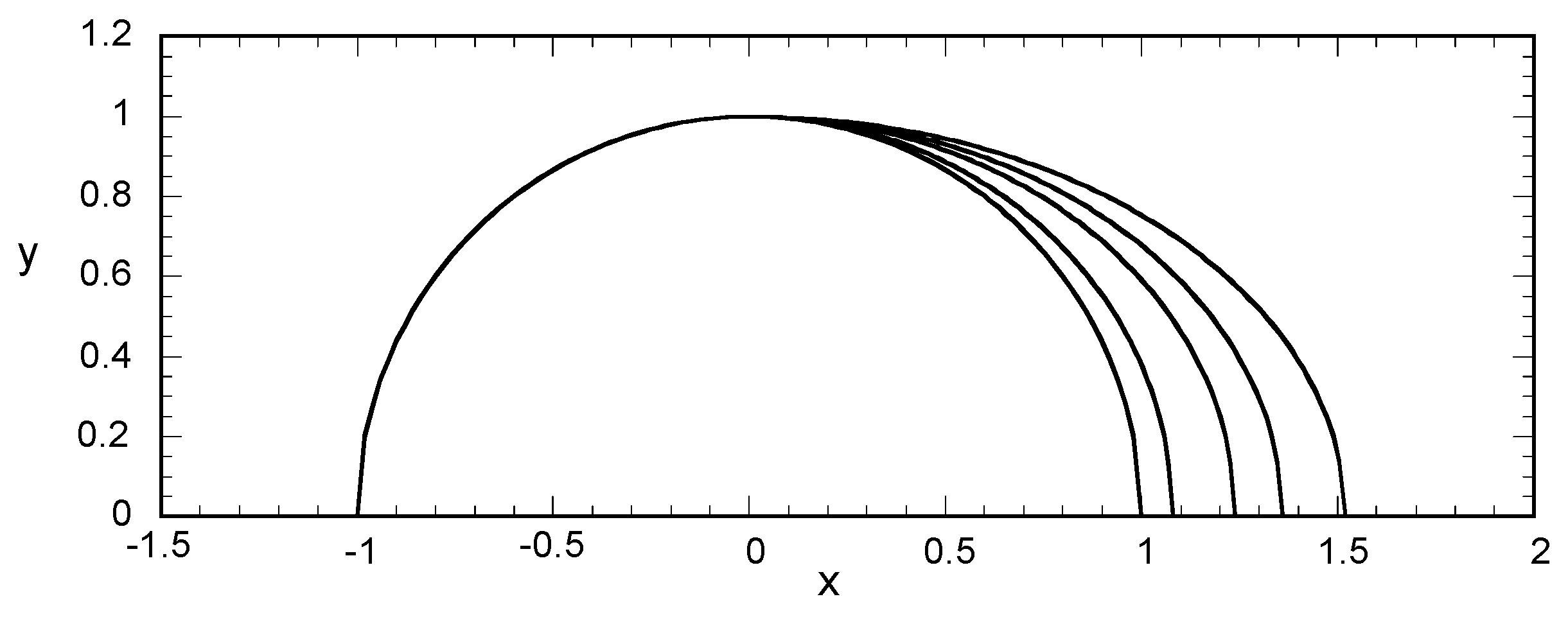
Figure 5. It is noted that a non-physical (but slight) overshoot of the contact angle appears close to the front edge of the droplet. However, this overshoot appears only for rear angles closer than 5°, so, in principle, the acquired profiles can be considered as acceptable. In that case, the consideration of a specific contact line shape is equivalent to the development of a contact line evolution model. The corresponding contact line shapes are shown in
Figure 6.
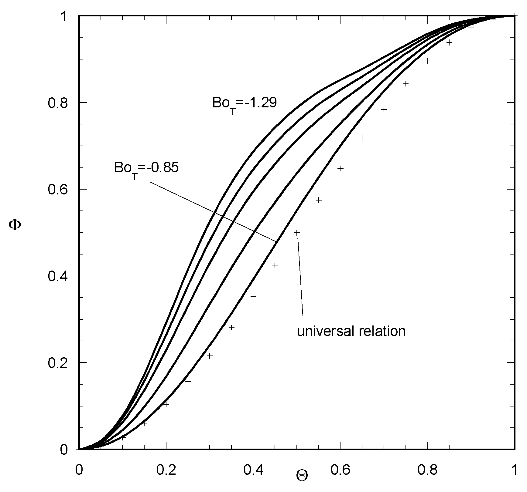
Inspired by the fact that the contact angle distribution proposed in [
13] under proper normalization can acquire a universal form, let us now try to apply a similar normalization here. The normalized contact angle is defined as Φ = (φ − φ
min)/(φ
max − φ
min), and the arclength along the contact line is replaced by the normalized azimuthal angle Θ = θ/π.
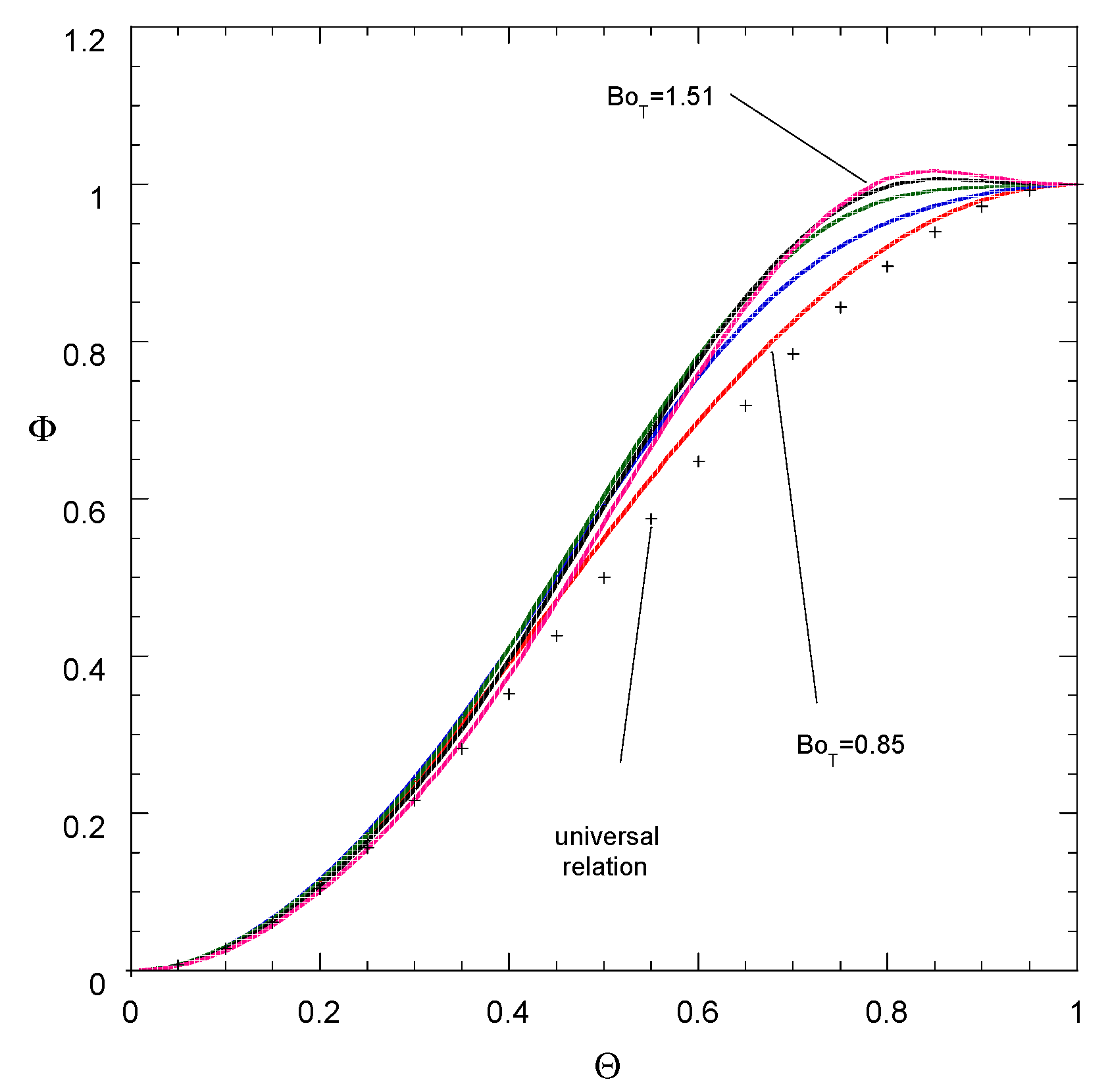
The contact angle distribution evolution in terms of normalized variables is shown in
Figure 7. It is obvious that the normalized contact angle distribution tends to a self-similar shape as the tangential Bond number increases. In the case of the initial contact angle being equal to the advancing one, the convergence to self-similarity confirms the universality proposal in [
13] converging at a faster rate. However, the resulting distribution is far from the universal one suggested in [
13], which takes the form Φ = 2(1 − Θ)
3 − 3(1 − Θ)
2 + 1 and also appears in
Figure 7. The universal shape adequately represents the actual distribution close to the two edges of the droplet, but there is a deviation in intermediate regions (especially in the elliptic part of the contact line). The universal shape is antisymmetric with respect to Θ = ½, which is a rather improbable behavior in light of the present results.
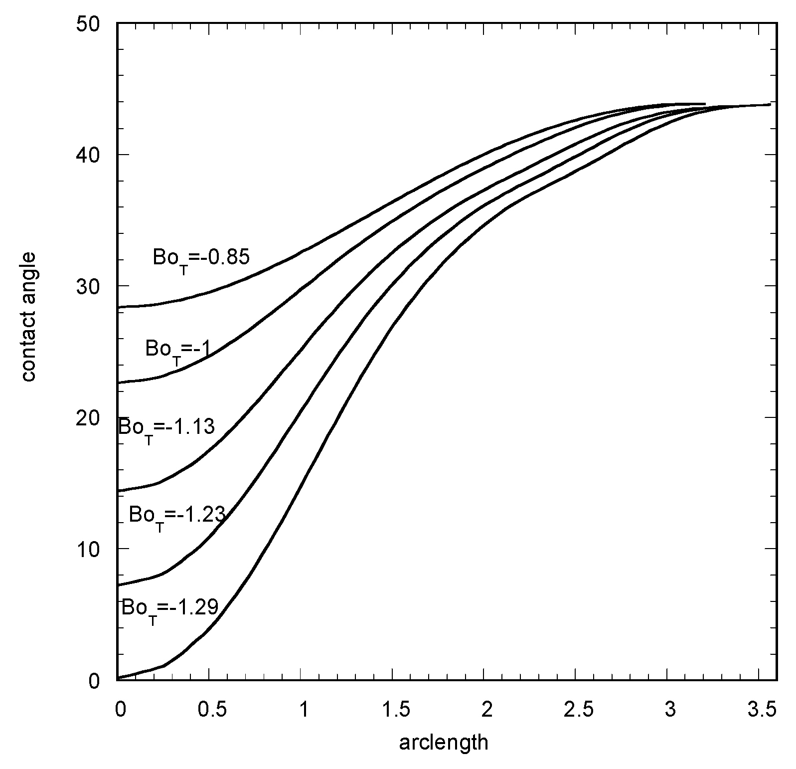
In order to demonstrate the versatility of the solution method and to shed more physical insight on the problem, the contact angle profiles at the contact line shown in
Figure 6 at the inception of spreading but with a force applying to the opposite direction are shown in
Figure 8. The corresponding normalized results are presented in
Figure 9. The spreading now starts for smaller (in absolute value) Bond numbers, as it is affected by the deformed contact line. It is noted than an elbow appears in the contact angle curve as the contact line deformation increases. The location of this elbow is at the position of transition of the contact line shape from circle to ellipsis. For larger Bo
T numbers, the evolution is mainly due to the increase of this elbow. In any case, universality does not appear in these curves. The presented example refers to conditions with no strict actual linearity but similar results for the normalized variables are taken for lower values of θ
A.
The fact is that for experimentally observed contact line shapes (an easy experimentally accessible feature) the resulting contact angle distribution (a very difficult experimentally accessible feature) does not obey the universal shape as suggested in the past. Apparently, the analysis here is in the linear limit, yet it is enough to invalidate the universality principle that should hold under all possible cases. The implication for the measurement techniques is that it is preferable for quasi-static state spreading on omniphilic surfaces to extract the contact angle distribution from the contact line shape than from direct contact angle measurements.
In summary, there are several methods to find the distribution of the contact angle for a sessile droplet spreading under the influence of bulk body forces. These methods start from the molecular scale (molecular dynamics), allowing consideration only of nanodroplets (for computational reasons) [
29] and continue with approaches based on precursor films and disjoining pressure profiles (still computationally intensive for three dimensional droplets) [
6]. The next level approaches are all based on the solution of the Young–Laplace equation, either combined to an evolution principle for the contact line, assuming a prescribed shape for the contact line, or for the contact angle profile. All approaches contain unknown parameters that have to be estimated by experimental data of contact line shapes. The suggestion in the present work is to use experimental information as much as possible, keeping the mathematical model for the contact line evolution simple. It is noted that the simultaneous variation of tangential and normal Bond numbers discussed in the present work is not experimentally straightforward. This is due to the fact that the relevant experimental studies are done on the basis of the rotation of horizontal drops or for drops on inclined plates. Recently, the device Kerveros [
28,
30] has been developed, which allows simultaneous control of the two Bond numbers by adjusting both the rotation frequency and inclination angle.


