Voxel-Based Finite Element Investigation of Micromechanics Models for Stiffness Prediction of Cross-Ply Laminates

Abstract

Laminate plate and shell structures with symmetric cross-ply configurations are widely used due to their high stiffness-to-weight ratio. However, conventional lamination theories rely on simplifying assumptions that may introduce inaccuracies. This study evaluates the predictive capability of such theories by integrating multiple micromechanics models with First-Order Shear Deformation Theory (FSDT), and comparing the results against voxel-based finite element modeling (VB-FEM), which serves as a high-fidelity numerical reference. A range of models—including Voigt–Reuss, Chamis, Halpin–Tsai, Bridging, and two iterative isotropized formulations—are assessed for unidirectional laminae with fiber volume fractions from 40% to 73%. Quantitative comparison reveals that while all models predict the longitudinal modulus accurately, significant deviations arise in predicting transverse and shear properties. The Bridging Model consistently yields the closest agreement with VB-FEM across all five elastic constants, maintaining accuracy even at high volume fractions where the modified Halpin–Tsai model begins to fail. Discrepancies in micromechanics-based lamina properties propagate to laminate-level stiffness predictions, highlighting the critical role of model selection. These findings establish VB-FEM as a valuable tool for validating analytical models and guide improved modeling strategies for laminated composite design.

1. Introduction

Laminate plate/shell structures are typically composed of multiple laminae with varying fiber orientations, allowing engineers to optimize their performance for specific load scenarios. These structures are widely used in engineering applications where a high stiffness-to-weight ratio is essential, such as in marine [1], civil [2], aerospace, military, and automotive sectors [3].

Considering their wide applications in critical engineering structures and industrial products, it is important to predict their mechanical behavior accurately. There are three primary methods to achieve this: analytical, numerical, and experimental. Given the multiple variables involved in designing laminates, such as fiber orientation, material properties, volume fraction [3], and fiber distribution [4], analytical formulas are preferred due to their computational efficiency. The analytical approach operates at two levels: macroscale and microscale. In macroscale analysis, laminate plate/shell theories are used to predict the laminate stiffness parameters based on the properties and stacking sequence of each lamina. In microscale analysis, micromechanics models are used to predict the properties of individual laminae, which are typically modeled as transversely isotropic unidirectional fiber composites characterized by five independent elastic constants.

Laminate plate/shell theories simplify three-dimensional problems into two dimensions by defining how deformation occurs through the thickness. Classical Laminate Theory (CLT), characterized by the Kirchhoff assumption [5], and First-Order Shear Deformation Theory (FSDT), represented by the Mindlin model [6], are widely used equivalent single-layer approaches for modeling laminated structures. CLT assumes that a normal line of the middle surface remains straight and perpendicular to the surface even after deformation [5]. As a result, transverse shear deformation is neglected, which makes the theory most appropriate for thin plates where shear effects are minimal. FSDT is an extension of CLT that accounts for the effects of transverse shear deformation [6] by relaxing the assumption of perpendicularity, making it suitable for analyzing thicker plates where transverse shear effects become significant.

To predict the properties of unidirectional laminae, several micromechanics models have been developed. Voigt–Reuss [7,8] is a simple and widely used method in the literature but known to be inaccurate for predicting the transverse Young’s modulus. Because of its simplicity, many models have been developed based on Voigt–Reuss to improve accuracy. Chamis [9] and Halpin–Tsai [10] are two popular modifications. Halpin and Tsai introduced two empirical parameters to account for environmental factors and proposed values for square distributions of fibers. Later, Hewitt and Malherbe [11] suggested alternative reinforcement factors for an E-glass and polyester resin system, and Giner et al. [12] proposed reinforcement factors for randomly distributed unidirectional fibers. There are also recent extensions of the Voigt–Reuss approach by Vignoli et al. [13,14], Kou et al. [15], and Luo [16].

In addition to Voigt–Reuss and its modifications, the Generalized Self-Consistent model [17,18], Mori–Tanaka model [19], and Bridging Model [20,21] are also widely applied in composite material analysis. The Generalized Self-Consistent model was initially proposed by Hashin and Rosen [18] and extended by Hashin [22] and Christensen and Lo [17]. Mori and Tanaka [19] developed a method that was reformulated by Benveniste [23] and closed-form expressions provided later by Abaimov et al. [24]. The Bridging Model introduces two empirical parameters to account for fiber packing geometry, and Wang and Huang [21] recommended a value that provided the most accurate overall results after investigating 18 composites.

Although analytical formulas are the most efficient, their accuracy differs in different situations, especially with high volume fractions of fibers and large differences between phase properties. For models with empirical parameters, the prediction accuracy of elastic properties is sensitive to the selection of these parameters, and curve fitting may be required to improve accuracy across different conditions. Huang et al. [20] and Wang et al. [21] investigated the sensitivity of elastic properties prediction to the selection of Bridging parameters, concluding that it can be significant for composites with large differences between phase properties. Therefore, analytical predictions alone are insufficient, and validation through numerical or experimental data is necessary. Though experimental data are the most reliable, they are cost- and time-intensive. Moreover, due to the large number of design parameters in laminate systems, there is a lack of experimental data to validate the analytical predictions, particularly for laminate composites.

Moreover, the stiffness parameters of a laminate depend on all five elastic properties of the lamina. However, most micromechanical models only focus on predicting some of these properties, and their accuracy is not consistent across all five properties, as investigated by [13,25]. Although most models accurately predict the longitudinal Young’s modulus and Poisson’s ratio, there is a lack of accuracy in the prediction of transverse Young’s modulus and shear moduli. Experimental studies on laminae (i.e., unidirectional composites) often focus only on predicting longitudinal Young’s modulus, rather than providing all the five elastic constants necessary for calculating the full stiffness matrix of laminate plates/shells.

Considering these limitations, numerical methods offer the benefit of generating a broader range of parametric results compared to experimental and analytical approaches. Combined with the rapid progress in computational technology, which has enabled advancements in numerical methods [26] and the need to represent complex microstructures in greater detail, numerical methods have become increasingly important and are applied in many studies of composite materials [27,28].

For numerical modeling, fiber distribution is a parameter that affects the elastic properties of laminate composites. Different fiber distributions, random and regular (including square and hexagonal arrangements), have been analyzed in comparative studies by several researchers [4,29,30]. The analysis of composites with regular fiber distributions does not require intensive computing, but actual fiber distributions in manufactured composites often exhibit irregularity due to process-induced variability. In this study, we approximate such irregularity using simulated microstructures generated by a non-overlapping random sequential algorithm, without claiming statistical equivalence to real materials. Thus, our simulations represent a class of irregular composites generated under a controlled protocol, rather than statistically validated random microstructures. Moreover, there are two modeling approaches: geometry-based finite element modeling (GB-FEM) and voxel-based finite element modeling (VB-FEM). In GB-FEM analysis, the geometry-based approaches can introduce complications in generating a high-quality mesh, as element shapes are determined by the object’s topology [31]. Although adaptive meshing can improve geometry representation, it may significantly increase computational cost and still does not always guarantee mesh quality [32]. Poor mesh quality can lead to increased numerical error in simulations. To address the challenges associated with GB-FEM, VB-FEM offers advantages, as it ensures mesh quality by generating a uniform mesh, followed by a material assignment. Luo [33] and Doitrand [34] compared the performance of these approaches, showing convergence in the computed elastic properties. While GB-FEM has lower computational costs when inclusions are large and regularly distributed, VB-FEM is similarly efficient—and sometimes even more so—for small, randomly distributed inclusions. These advantages have led to VB-FEM’s application in diverse areas [34,35,36].

Despite the extensive literature on micromechanics models and laminate theories, few studies have systematically compared a broad spectrum of classical, empirical, and recently proposed micromechanics models against high-fidelity voxel-based finite element modeling (VB-FEM). This study addresses that gap by evaluating how the accuracy of lamina property predictions—particularly for transverse and shear moduli—affects the stiffness predictions of symmetric laminate plates using First-Order Shear Deformation Theory (FSDT). In this study, first, for unidirectional composites, the accuracy of various micromechanics models is evaluated by comparing their predictions against both experimental data and voxel-based finite element modeling. For high volume fractions, varying fiber diameters are used to capture realistic packing effects at different scales. The evaluated micromechanics models include Voigt–Reuss (VR), Chamis, Halpin–Tsai (HT), Halpin–Tsai modified (HTm), Generalized Self-Consistent (GSC), Mori–Tanaka (MT), and the Bridging Model (Br). Additionally, two iterative models, Iterative Isotropized Voigt–Reuss bounds (Iter-Iso-VR) and Iterative Isotropized Hashin–Shtrikman bounds (Iter-Iso-HS), originally proposed by Luo [16] for predicting the elastic properties of particulate composites, are also included. The lamina stiffness parameters are then used to determine the elements in the laminate stiffness matrix as defined by FSDT, i.e., the in-plane stiffness matrix (A), the bending stiffness matrix (D), and the transverse shear stiffness matrix (H). The predictions of laminate plates/shells’ effective properties obtained from FSDT based on the selected micromechanics models are then compared to those derived from VB-FEM. The predictive capability of the analytical laminate formulation is assessed, providing insights into its applicability for designing and analyzing laminated composite structures.

2. First-Order Shear Deformation Theory and Micromechanical Models

In this section, we outline the First-Order Shear Deformation Theory (FSDT) as the analytical basis for predicting laminate plate and shell stiffness—including the derivation of the in-plane (A), bending (D), and transverse shear (H) stiffness matrices—and then introduce the suite of micromechanical models for estimating the elastic properties of unidirectional laminae, from classical Voigt–Reuss bounds to advanced self-consistent and empirical formulations. The symbols used in the equations and their interpretations are listed in

Table 1. Symbols used in the equations and their corresponding interpretations.

${\mathrm{A}}_{\mathrm{i}\mathrm{j}}$	In-plane stiffness matrix	${\mathrm{K}}_{23}^{\mathrm{f}}$	Fiber out-of-plane bulk modulus
${\mathrm{B}}_{\mathrm{i}\mathrm{j}}$	Coupling matrix	${\mathrm{K}}^{\mathrm{m}}$	Matrix bulk modulus
${\mathrm{D}}_{\mathrm{i}\mathrm{j}}$	Bending stiffness matrix	${\mathrm{K}}_{\mathrm{U}}^{\left(\mathrm{i}\right)}$	The upper bound of bulk modulus in i-th iteration
${\mathrm{E}}_1$	Longitudinal elastic modulus	${\mathrm{K}}_{\mathrm{L}}^{\left(\mathrm{i}\right)}$	The lower bound of bulk modulus in i-th iteration
${\mathrm{E}}_2$	Transversal elastic modulus	${\mathrm{Q}}^{\mathrm{*}}$	Stiffness matrix derived from $S^{\mathrm{*}}$
${\mathrm{E}}_1^{\mathrm{f}}$	Fiber longitudinal elastic modulus	${\left({\overline{\mathrm{Q}}}_{\mathrm{i}\mathrm{j}}\right)}_{\mathrm{k}}$	Transformed reduced stiffness matrix of k-th lamina into the global coordinate system of the laminate
${\mathrm{E}}_2^{\mathrm{f}}$	Fiber transversal elastic modulus	S	Compliance matrix
${\mathrm{E}}^{\mathrm{m}}$	Matrix elastic modulus	$S^{\mathrm{*}}$	Remaining two equations to complete the compliance matric
${\mathrm{E}}_{\mathrm{U}}^{\left(\mathrm{i}\right)}$	The upper bound of elastic modulus in ith iteration	t	Thickness of laminate
${\mathrm{E}}_{\mathrm{L}}^{\left(\mathrm{i}\right)}$	The lower bound of elastic modulus in ith iteration	$\mathrm{T}\left(\mathsf{\theta }\right)$	Transformation matrix
${\mathrm{E}}_x^{\mathrm{f}}{,\mathrm{E}}_y^{\mathrm{f}}$	Effective flexural Young’s moduli of laminate	${\mathrm{t}}_{\mathrm{k}}$	Thickness of k-th lamina
${\mathrm{f}}_1,{\mathrm{f}}_2$	Phase volume fraction	${\mathsf{\nu }}_{12}$	In-plane Poisson’s ratio
${\mathrm{G}}_{12}$	In-plane shear modulus	${\mathsf{\nu }}_{12}^{\mathrm{f}}$	Fiber in-plane Poisson’s ratio
${\mathrm{G}}_{23}$	Out-of-plane shear modulus	${\mathsf{\nu }}^{\mathrm{m}}$	Matrix Poisson’s ratio
${\mathrm{G}}_{12}^{\mathrm{f}}$	Fiber in-plane shear modulus	${\mathrm{V}}_{\mathrm{f}}$	Fiber volume fraction
${\mathrm{G}}_{23}^{\mathrm{f}}$	Fiber out-of-plane shear modulus	${\overline{\mathrm{z}}}_{\mathrm{k}}$	Coordinate of the middle surface of the k-th lamina
${\mathrm{G}}^{\mathrm{m}}$	Matrix shear modulus	σ	Normal stress
${\mathrm{G}}_{\mathrm{U}}^{\left(\mathrm{i}\right)}$	The upper bound of shear modulus in i-th iteration	ε	Normal strain
${\mathrm{G}}_{\mathrm{L}}^{\left(\mathrm{i}\right)}$	The lower bound of shear modulus in i-th iteration	τ	Shear stress
${\mathrm{H}}_{\mathrm{i}\mathrm{j}}$	Transverse shear stiffness matrix	γ	Shear strain
${\mathrm{K}}_{23}$	Out-of-plane bulk modulus	θ	Fiber orientation angle

.

2.1. Laminate Plate/Shell Stiffness Formulations

The in-plane and out-of-plane behavior of laminates is described by the A, B, D, and H stiffness matrices. Under the First-Order Shear Deformation Theory (FSDT) assumptions, the normal to the undeformed mid-surface remains straight but rotates during deformation, while thickness changes are neglected [5]. By integrating each layer’s contribution across the laminate thickness, one obtains the in-plane stiffness matrix (A), the extension–bending coupling matrix (B), the bending stiffness matrix (D), and the transverse shear stiffness matrix (H), as formulated in Equations (1)–(4).

$${\mathrm{A}}_{\mathrm{i}\mathrm{j}}=\sum _{\mathrm{k}=1}^{\mathrm{N}}{\left({\overline{\mathrm{Q}}}_{\mathrm{i}\mathrm{j}}\right)}_{\mathrm{k}}{\mathrm{t}}_{\mathrm{k}}; \mathrm{i},\mathrm{j}=\mathrm{1,2},6$$

(1)

$${\mathrm{B}}_{\mathrm{i}\mathrm{j}}=\sum _{\mathrm{k}=1}^{\mathrm{N}}{\left({\overline{\mathrm{Q}}}_{\mathrm{i}\mathrm{j}}\right)}_{\mathrm{k}}{\mathrm{t}}_{\mathrm{k}}{\overline{\mathrm{z}}}_{\mathrm{k}}; \mathrm{i},\mathrm{j}=\mathrm{1,2},6$$

(2)

$${\mathrm{D}}_{\mathrm{i}\mathrm{j}}=\sum _{\mathrm{k}=1}^{\mathrm{N}}{\left({\overline{\mathrm{Q}}}_{\mathrm{i}\mathrm{j}}\right)}_{\mathrm{k}}\left({\mathrm{t}}_{\mathrm{k}}{\overline{\mathrm{z}}}_{\mathrm{k}}^2+{\displaystyle \frac{{\mathrm{t}}_{\mathrm{k}}^3}{12}}\right); \mathrm{i},\mathrm{j}=\mathrm{1,2},6$$

(3)

$${\mathrm{H}}_{\mathrm{i}\mathrm{j}}={\displaystyle \frac{5}{4}}\sum _{\mathrm{k}=1}^{\mathrm{N}}{\left({\overline{\mathrm{Q}}}_{\mathrm{i}\mathrm{j}}^{\mathrm{*}}\right)}_{\mathrm{k}}[{\mathrm{t}}_{\mathrm{k}}-{\displaystyle \frac{4}{{\mathrm{t}}^2}}({\mathrm{t}}_{\mathrm{k}}{\overline{\mathrm{z}}}_{\mathrm{k}}^2+{\displaystyle \frac{{\mathrm{t}}_{\mathrm{k}}^3}{12}}); \mathrm{i},\mathrm{j}=\mathrm{4,5}$$

(4)

Here, N denotes the total number of laminae. t is the overall laminate thickness and t_k is the thickness of k-th lamina. The coordinate ${\overline{\mathrm{z}}}_{\mathrm{k}}$ locates the middle surface of that lamina. Finally, ${\left({\overline{\mathrm{Q}}}_{\mathrm{i}\mathrm{j}}\right)}_{\mathrm{k}}$ is the k-th lamina’s reduced stiffness matrix transformed into the laminate’s global coordinate system via the rotation matrices in Equations (5)–(7) [5].

$$\overline{\mathrm{Q}}={\left[\mathrm{T}\right]}^{-1}\left[\mathrm{Q}\right]{\left[\mathrm{T}\right]}^{-\mathrm{T}}$$

(5)

$$\mathrm{T}(\mathsf{\theta })=\left[\begin{array}{ccc}{\cos \mathsf{\theta }}^2& {\sin \mathsf{\theta }}^2& 2\cos \mathsf{\theta }\sin \mathsf{\theta }\\ {\sin \mathsf{\theta }}^2& {\cos \mathsf{\theta }}^2& -2\cos \mathsf{\theta }\sin \mathsf{\theta }\\ -\cos \mathsf{\theta }\sin \mathsf{\theta }& \cos \mathsf{\theta }\sin \mathsf{\theta }& {\cos \mathsf{\theta }}^2-{\sin \mathsf{\theta }}^2\end{array}\right]$$

(6)

$${\mathrm{T}}^{\mathrm{*}}=\left[\begin{array}{cc}\cos \mathsf{\theta }& \sin \mathsf{\theta }\\ -\sin \mathsf{\theta }& \cos \mathsf{\theta }\end{array}\right]$$

(7)

The reduced stiffness matrix of a transversely isotropic unidirectional lamina is obtained by inverting the compliance matrices in Equations (8) and (9) [5]. Those compliance matrices incorporate the five independent elastic constants predicted by the chosen micromechanical models.

$$\mathrm{S}=\left[\begin{array}{ccc}{\displaystyle \frac{1}{{\mathrm{E}}_1}}& -{\displaystyle \frac{{\mathsf{\upsilon }}_{12}}{{\mathrm{E}}_1}}& 0\\ -{\displaystyle \frac{{\mathsf{\upsilon }}_{12}}{{\mathrm{E}}_1}}& {\displaystyle \frac{1}{{\mathrm{E}}_2}}& 0\\ 0& 0& {\displaystyle \frac{1}{{\mathrm{G}}_{12}}}\end{array}\right]$$

(8)

$${\mathrm{S}}^{\mathrm{*}}=\left[\begin{array}{cc}{\displaystyle \frac{1}{{\mathrm{G}}_{23}}}& 0\\ 0& {\displaystyle \frac{1}{{\mathrm{G}}_{12}}}\end{array}\right]$$

(9)

For a balanced and symmetric laminate (A₁₃ = A₂₃ = 0), the in-plane elastic properties can be directly obtained from the A matrix using Equations (10)–(13).

$${\mathrm{E}}_{\mathrm{x}\mathrm{x}}={\displaystyle \frac{{\mathrm{A}}_{11}{\mathrm{A}}_{22}-{\mathrm{A}}_{12}^2}{\mathrm{t}{\mathrm{A}}_{22}}}$$

(10)

$${\mathrm{E}}_{\mathrm{y}\mathrm{y}}={\displaystyle \frac{{\mathrm{A}}_{11}{\mathrm{A}}_{22}-{\mathrm{A}}_{12}^2}{\mathrm{t}{\mathrm{A}}_{11}}}$$

(11)

$${\mathsf{\nu }}_{\mathrm{x}\mathrm{y}}={\displaystyle \frac{{\mathrm{A}}_{12}}{{\mathrm{A}}_{22}}}$$

(12)

$${\mathrm{G}}_{\mathrm{x}\mathrm{y}}={\displaystyle \frac{{\mathrm{A}}_{33}}{t}}$$

(13)

For laminates that are symmetric about the mid-surface, the coupling matrix B is identically zero. The bending stiffness terms therefore reduce to Equations (14)–(17), with D₁₃ and D₂₃ omitted for balanced, symmetric layups.

$${\mathrm{E}}_{\mathrm{x}}^{\mathrm{f}}=12{\displaystyle \frac{{\mathrm{D}}_{11}{\mathrm{D}}_{22}-{\mathrm{D}}_{12}^2}{{\mathrm{t}}^3{\mathrm{D}}_{22}}}$$

(14)

$${\mathrm{E}}_{\mathrm{y}}^{\mathrm{f}}=12{\displaystyle \frac{{\mathrm{D}}_{11}{\mathrm{D}}_{22}-{\mathrm{D}}_{12}^2}{{\mathrm{t}}^3{\mathrm{D}}_{11}}}$$

(15)

$${\mathsf{\nu }}_{\mathrm{x}\mathrm{y}}^{\mathrm{f}}={\displaystyle \frac{{\mathrm{D}}_{12}}{{\mathrm{D}}_{22}}}$$

(16)

$${\mathrm{G}}_{\mathrm{x}\mathrm{y}}^{\mathrm{f}}=12{\displaystyle \frac{{\mathrm{D}}_{33}}{{\mathrm{t}}^3}}$$

(17)

The transverse shear moduli are obtained from the H matrix using Equations (18) and (19).

$${\mathrm{G}}_{\mathrm{y}\mathrm{z}}={\displaystyle \frac{{\mathrm{H}}_{11}}{\mathrm{t}}}$$

(18)

$${\mathrm{G}}_{\mathrm{x}\mathrm{z}}={\displaystyle \frac{{\mathrm{H}}_{22}}{\mathrm{t}}}$$

(19)

2.2. Micromechanics Models for Unidirectional Laminae

To predict the elastic properties of unidirectional laminae, a variety of micromechanical models have been developed. Here, we briefly describe the models considered in this study and present their governing equations: Voigt–Reuss (VR), Chamis, Halpin–Tsai (HT) and its modified form (HTm), Generalized Self-Consistent (GSC), Mori–Tanaka (MT), the Bridging Model (Br), and two recent iterative schemes—the Iterative Isotropized Voigt–Reuss bounds (Iter-Iso-VR) and the Iterative Isotropized Hashin–Shtrikman bounds (Iter-Iso-HS).

Micromechanics models serve as a critical link in multiscale modeling by homogenizing the elastic behavior of fiber and matrix constituents to predict the effective properties of unidirectional laminae. These homogenized properties—typically including ${\mathrm{E}}_1$, ${\mathrm{E}}_2$, ${\mathrm{G}}_{12}$, ${\mathrm{G}}_{23}$, and ${\mathsf{\nu }}_{12}$—are then used as inputs to analytical laminate theories such as First-Order Shear Deformation Theory (FSDT). This approach enables the efficient estimation of global laminate stiffness without the need to explicitly resolve microstructural geometry in every simulation.

2.2.1. Voigt–Reuss Model

The Voigt model assumes that the fiber, matrix, and composite all have the same strain [5]. Consequently, the longitudinal elastic modulus (E₁) and the in-plane Poisson ratio (v₁₂) are given by Equations (20) and (21).

$${\mathrm{E}}_1={\mathrm{E}}_1^{\mathrm{f}}{\mathrm{V}}_{\mathrm{f}}+\left(1-{\mathrm{V}}_{\mathrm{f}}\right){\mathrm{E}}^{\mathrm{m}}$$

(20)

$${\mathsf{\nu }}_{12}={\mathsf{\nu }}_{12}^{\mathrm{f}}{\mathrm{V}}_{\mathrm{f}}+\left(1-{\mathrm{V}}_{\mathrm{f}}\right){\mathsf{\nu }}^{\mathrm{m}}$$

(21)

where directions 1 and 2 correspond to the longitudinal and transverse orientations, respectively.

In contrast, the Reuss model assumes uniform stress across the fiber, matrix, and composite [5]. Under this assumption, the transverse elastic modulus (E₂), the in-plane shear modulus (G₁₂), and the out-of-plane shear modulus (G₂₃) are given by Equations (22)–(24) [15].

$${\mathrm{E}}_2={\displaystyle \frac{{\mathrm{E}}_2^{\mathrm{f}} {\mathrm{E}}^{\mathrm{m}}}{{\mathrm{E}}_2^{\mathrm{f}}\left(1-{\mathrm{V}}_{\mathrm{f}}\right)+{\mathrm{E}}^{\mathrm{m}}{\mathrm{V}}_{\mathrm{f}}}}$$

(22)

$${\mathrm{G}}_{12}={\displaystyle \frac{{\mathrm{G}}_{12}^{\mathrm{f}} {\mathrm{G}}^{\mathrm{m}}}{{\mathrm{G}}_{12}^{\mathrm{f}}\left(1-{\mathrm{V}}_{\mathrm{f}}\right)+{\mathrm{G}}^{\mathrm{m}}{\mathrm{V}}_{\mathrm{f}}}}$$

(23)

$${\mathrm{G}}_{23}={\displaystyle \frac{{\mathrm{G}}_{23}^{\mathrm{f}} {\mathrm{G}}^{\mathrm{m}}}{{\mathrm{G}}_{23}^{\mathrm{f}}\left(1-{\mathrm{V}}_{\mathrm{f}}\right)+{\mathrm{G}}^{\mathrm{m}}{\mathrm{V}}_{\mathrm{f}}}}$$

(24)

2.2.2. Hashin–Strikman Equations

The Hashin–Strikman bounds in Equations (25)–(28) [37] provide upper and lower limits for a composite’s effective bulk and shear moduli. The corresponding Young’s modulus is then obtained from these bounds using Equation (29).

$${\mathrm{G}}_{\mathrm{L}}={\mathrm{G}}_{\mathrm{m}}+{\displaystyle \frac{{\mathrm{V}}_{\mathrm{f}}}{\left[\frac{1}{{\mathrm{G}}_{\mathrm{f}}-{\mathrm{G}}_{\mathrm{m}}}+\frac{6\left(1-{\mathrm{V}}_{\mathrm{f}}\right)({\mathrm{K}}_{\mathrm{m}}+2{\mathrm{G}}_{\mathrm{m}})}{{5\mathrm{G}}_{\mathrm{m}}{(3\mathrm{K}}_{\mathrm{m}}+{4\mathrm{G}}_{\mathrm{m}})}\right]}}$$

(25)

$${\mathrm{G}}_{\mathrm{U}}={\mathrm{G}}_{\mathrm{f}}+{\displaystyle \frac{\left(1-{\mathrm{V}}_{\mathrm{f}}\right)}{\left[\frac{1}{{\mathrm{G}}_{\mathrm{m}}-{\mathrm{G}}_{\mathrm{f}}}+\frac{6{\mathrm{V}}_{\mathrm{f}}({\mathrm{K}}_{\mathrm{f}}+2{\mathrm{G}}_{\mathrm{f}})}{{5\mathrm{G}}_{\mathrm{f}}{(3\mathrm{K}}_{\mathrm{f}}+{4\mathrm{G}}_{\mathrm{f}})}\right]}}$$

(26)

$${\mathrm{K}}_{\mathrm{L}}={\mathrm{K}}_{\mathrm{m}}+{\displaystyle \frac{{\mathrm{V}}_{\mathrm{f}}}{\left[\frac{1}{{\mathrm{K}}_{\mathrm{f}}-{\mathrm{K}}_{\mathrm{m}}}+\frac{\left(1-{\mathrm{V}}_{\mathrm{f}}\right)}{{\mathrm{K}}_{\mathrm{m}}+\frac{4}{3}{\mathrm{G}}_{\mathrm{m}})}\right]}}$$

(27)

$${\mathrm{K}}_{\mathrm{U}}={\mathrm{K}}_{\mathrm{f}}+{\displaystyle \frac{\left(1-{\mathrm{V}}_{\mathrm{f}}\right)}{\left[\frac{1}{{\mathrm{K}}_{\mathrm{m}}-{\mathrm{K}}_{\mathrm{f}}}+\frac{{\mathrm{V}}_{\mathrm{f}}}{{\mathrm{K}}_{\mathrm{f}}+\frac{4}{3}{\mathrm{G}}_{\mathrm{f}})}\right]}}$$

(28)

$$\mathrm{E}={\displaystyle \frac{9\mathrm{K}\mathrm{G}}{3\mathrm{K}+\mathrm{G}}}$$

(29)

2.2.3. Chamis Model

The Chamis model employs the Voigt–Reuss equations to predict the longitudinal modulus (E₁) and in-plane Poisson’s ratio (ν₁₂); the transverse modulus (E₂), in-plane shear modulus (G₁₂), and the out-of-plane shear modulus (G₂₃) are then obtained from Equations (30)–(32) [9].

$${\mathrm{E}}_2={\displaystyle \frac{{\mathrm{E}}^{\mathrm{m}}}{1-\sqrt{{\mathrm{V}}_{\mathrm{f}}}[1-({\mathrm{E}}^{\mathrm{m}}/{\mathrm{E}}_2^{\mathrm{f}}\left)\right]}}$$

(30)

$${\mathrm{G}}_{12}={\displaystyle \frac{{\mathrm{G}}^{\mathrm{m}}}{1-\sqrt{{\mathrm{V}}_{\mathrm{f}}}[1-({\mathrm{G}}^{\mathrm{m}}/{\mathrm{G}}_{12}^{\mathrm{f}}\left)\right]}}$$

(31)

$${\mathrm{G}}_{23}={\displaystyle \frac{{\mathrm{G}}^{\mathrm{m}}}{1-\sqrt{{\mathrm{V}}_{\mathrm{f}}}[1-({\mathrm{G}}^{\mathrm{m}}/{\mathrm{G}}_{23}^{\mathrm{f}}\left)\right]}}$$

(32)

2.2.4. Halpin–Tsai Model

The Halpin–Tsai model applies the Voigt–Reuss expressions to predict the longitudinal modulus (E₁) and in-plane Poisson’s ratio (ν₁₂) and then introduces two empirical parameters—${\mathsf{\zeta }}_{{\mathrm{E}}_2}$ and ${\mathsf{\zeta }}_{{\mathrm{G}}_2}$—to account for environmental and packing effects when estimating the transverse modulus (E₂) and in-plane shear modulus (G₁₂). Equations (33)–(38) detail these relationships, with the original recommendations ${\mathsf{\zeta }}_{{\mathrm{E}}_2}=2$ and ${\mathsf{\zeta }}_{{\mathrm{G}}_2}=1$ for a square-array fiber distribution [10].

$${\mathrm{E}}_2={\mathrm{E}}^{\mathrm{m}}\left({\displaystyle \frac{1+{\mathsf{\zeta }}_{{\mathrm{E}}_2}{\mathsf{\eta }}_{{\mathrm{E}}_2}{\mathrm{V}}_{\mathrm{f}}}{1-{\mathsf{\eta }}_{{\mathrm{E}}_2}{\mathrm{V}}_{\mathrm{f}}}}\right)$$

(33)

$${\mathrm{G}}_{12}={\mathrm{G}}^{\mathrm{m}}\left({\displaystyle \frac{1+{\mathsf{\zeta }}_{{\mathrm{G}}_{12}}{\mathsf{\eta }}_{{\mathrm{G}}_{12}}{\mathrm{V}}_{\mathrm{f}}}{1-{\mathsf{\eta }}_{{\mathrm{G}}_{12}}{\mathrm{V}}_{\mathrm{f}}}}\right)$$

(34)

$${\mathsf{\eta }}_{{\mathrm{E}}_2}={\displaystyle \frac{({\mathrm{E}}_2^{\mathrm{f}}/{\mathrm{E}}^{\mathrm{m}})-1}{({\mathrm{E}}_2^{\mathrm{f}}/{\mathrm{E}}^{\mathrm{m}})+{\mathsf{\zeta }}_{{\mathrm{E}}_2}}}$$

(35)

$${\mathsf{\eta }}_{{\mathrm{G}}_{12}}={\displaystyle \frac{({\mathrm{G}}_{12}^{\mathrm{f}}/{\mathrm{G}}^{\mathrm{m}})-1}{({\mathrm{G}}_{12}^{\mathrm{f}}/{\mathrm{G}}^{\mathrm{m}})+{\mathsf{\zeta }}_{{\mathrm{G}}_{12}}}}$$

(36)

$${\mathsf{\zeta }}_{{\mathrm{E}}_2}=2$$

(37)

$${\mathsf{\zeta }}_{{\mathrm{G}}_{12}}=1$$

(38)

2.2.5. Halpin–Tsai Modified Model

The modified Halpin–Tsai model introduces a revised empirical parameter, ${\mathsf{\zeta }}_{{\mathrm{E}}_2}$, to account for randomly distributed fibers; its functional form is given in Equation (39) [12].

$${\mathsf{\zeta }}_{{\mathrm{E}}_2}=\left\{\begin{array}{c}4.924-35.888{\mathrm{V}}_{\mathrm{f}}+125.118{\mathrm{V}}_{\mathrm{f}}^2-145.121{\mathrm{V}}_{\mathrm{f}}^3 \mathrm{if} {\mathrm{V}}_{\mathrm{f}}<0.3\\ 1.5+5500{\mathrm{V}}_{\mathrm{f}}^{18} \mathrm{if} {\mathrm{V}}_{\mathrm{f}}\ge 0.3\end{array}\right.$$

(39)

2.2.6. Generalized Self-Consistent

The Generalized Self-Consistent model assumes a three-phase inclusion geometry, with its governing equations provided in Equations (40)–(62) [38]:

$${\mathrm{E}}_1={\mathrm{E}}_1^{\mathrm{f}}{\mathrm{V}}_{\mathrm{f}}+{\mathrm{E}}^{\mathrm{m}}\left(1-{\mathrm{V}}_{\mathrm{f}}\right)+{\displaystyle \frac{4{\mathrm{V}}_{\mathrm{f}}(1-{\mathrm{V}}_{\mathrm{f}}){\left({\mathsf{\nu }}_{12}^{\mathrm{f}}-{\mathsf{\nu }}^{\mathrm{m}}\right)}^2}{\frac{(1-{\mathrm{V}}_{\mathrm{f}})}{{\mathrm{K}}_{23}^{\mathrm{f}}}+\frac{{\mathrm{V}}_{\mathrm{f}}}{{\mathrm{K}}^{\mathrm{m}}}+\frac{1}{{\mathrm{G}}^{\mathrm{m}}}}}$$

(40)

$${\mathsf{\nu }}_{12}={\mathsf{\nu }}_{12}^{\mathrm{f}}{\mathrm{V}}_{\mathrm{f}}+{\mathsf{\nu }}^{\mathrm{m}}\left(1-{\mathrm{V}}_{\mathrm{f}}\right)+{\displaystyle \frac{{\mathrm{V}}_{\mathrm{f}}\left(1-{\mathrm{V}}_{\mathrm{f}}\right){\left({\mathsf{\nu }}_{12}^{\mathrm{f}}-{\mathsf{\nu }}^{\mathrm{m}}\right)}^2\left(\frac{1}{{\mathrm{K}}^{\mathrm{m}}}-\frac{1}{{\mathrm{K}}_{23}^{\mathrm{f}}}\right)}{\frac{(1-{\mathrm{V}}_{\mathrm{f}})}{{\mathrm{K}}_{23}^{\mathrm{f}}}+\frac{{\mathrm{V}}_{\mathrm{f}}}{{\mathrm{K}}^{\mathrm{m}}}+\frac{1}{{\mathrm{G}}^{\mathrm{m}}}}}$$

(41)

$${\mathrm{K}}_{23}={\mathrm{K}}^{\mathrm{m}}+{\displaystyle \frac{{\mathrm{V}}_{\mathrm{f}}}{\frac{1}{{\mathrm{K}}_{23}^{\mathrm{f}}-{\mathrm{K}}^{\mathrm{m}}}+\frac{{1-\mathrm{V}}_{\mathrm{f}}}{{\mathrm{K}}^{\mathrm{m}}+{\mathrm{G}}^{\mathrm{m}}}}}$$

(42)

$${\mathrm{G}}_{12}={\mathrm{G}}^{\mathrm{m}}{\displaystyle \frac{{\mathrm{G}}_{12}^{\mathrm{f}}\left(1+{\mathrm{V}}_{\mathrm{f}}\right)+{\mathrm{G}}^{\mathrm{m}}\left(1-{\mathrm{V}}_{\mathrm{f}}\right)}{{\mathrm{G}}_{12}^{\mathrm{f}}\left(1-{\mathrm{V}}_{\mathrm{f}}\right)+{\mathrm{G}}^{\mathrm{m}}\left(1+{\mathrm{V}}_{\mathrm{f}}\right)}}$$

(43)

$${\mathrm{G}}_{23}={\mathrm{G}}^{\mathrm{m}}\left({\displaystyle \frac{-\mathrm{B}+\sqrt{{\mathrm{B}}^2-4\mathrm{A}\mathrm{C}}}{2\mathrm{A}}}\right)$$

(44)

$$\mathrm{A}={\mathrm{a}}_0+{\mathrm{a}}_1{\mathrm{V}}_{\mathrm{f}}+{\mathrm{a}}_2{\mathrm{V}}_{\mathrm{f}}^2+{\mathrm{a}}_3{\mathrm{V}}_{\mathrm{f}}^3+{\mathrm{a}}_4{\mathrm{V}}_{\mathrm{f}}^4$$

(45)

$$\mathrm{B}={\mathrm{b}}_0+{\mathrm{b}}_1{\mathrm{V}}_{\mathrm{f}}+{\mathrm{b}}_2{\mathrm{V}}_{\mathrm{f}}^2+{\mathrm{b}}_3{\mathrm{V}}_{\mathrm{f}}^3+{\mathrm{b}}_4{\mathrm{V}}_{\mathrm{f}}^4$$

(46)

$$\mathrm{C}={\mathrm{c}}_0+{\mathrm{c}}_1{\mathrm{V}}_{\mathrm{f}}+{\mathrm{c}}_2{\mathrm{V}}_{\mathrm{f}}^2+{\mathrm{c}}_3{\mathrm{V}}_{\mathrm{f}}^3+{\mathrm{c}}_4{\mathrm{V}}_{\mathrm{f}}^4$$

(47)

$${\mathrm{a}}_0=-2{\left({\mathrm{G}}^{\mathrm{m}}\right)}^2(2{\mathrm{G}}^{\mathrm{m}}+{\mathrm{K}}^{\mathrm{m}})[2{\mathrm{G}}_{23}^{\mathrm{f}}{\mathrm{G}}^{\mathrm{m}}+{\mathrm{K}}_{23}^{\mathrm{f}}({\mathrm{G}}_{23}^{\mathrm{f}}+{\mathrm{G}}^{\mathrm{m}}\left)\right][2{\mathrm{G}}_{23}^{\mathrm{f}}{\mathrm{G}}^{\mathrm{m}}+{\mathrm{K}}^{\mathrm{m}}({\mathrm{G}}_{23}^{\mathrm{f}}+{\mathrm{G}}^{\mathrm{m}}\left)\right]$$

(48)

$${\mathrm{a}}_1=8{\left({\mathrm{G}}^{\mathrm{m}}\right)}^2({\mathrm{G}}_{23}^{\mathrm{f}}-{\mathrm{G}}^{\mathrm{m}})[2{\mathrm{G}}_{23}^{\mathrm{f}}{\mathrm{G}}^{\mathrm{m}}+{\mathrm{K}}_{23}^{\mathrm{f}}({\mathrm{G}}_{23}^{\mathrm{f}}+{\mathrm{G}}^{\mathrm{m}}\left)\right][{\left({\mathrm{G}}^{\mathrm{m}}\right)}^2+{\mathrm{G}}^{\mathrm{m}}{\mathrm{K}}^{\mathrm{m}}+{\left({\mathrm{K}}^{\mathrm{m}}\right)}^2]$$

(49)

$${\mathrm{a}}_2=-12{\left({\mathrm{G}}^{\mathrm{m}}\right)}^2{\left({\mathrm{K}}^{\mathrm{m}}\right)}^2({\mathrm{G}}_{23}^{\mathrm{f}}-{\mathrm{G}}^{\mathrm{m}})[2{\mathrm{G}}_{23}^{\mathrm{f}}{\mathrm{G}}^{\mathrm{m}}+{\mathrm{K}}_{23}^{\mathrm{f}}({\mathrm{G}}_{23}^{\mathrm{f}}+{\mathrm{G}}^{\mathrm{m}}\left)\right]$$

(50)

$$\begin{gathered} {\mathrm{a}}_3=8{\left({\mathrm{G}}^{\mathrm{m}}\right)}^2\{{\left({\mathrm{G}}_{23}^{\mathrm{f}}{\mathrm{G}}^{\mathrm{m}}\right)}^2{\mathrm{K}}_{23}^{\mathrm{f}}+{\left({\mathrm{G}}_{23}^{\mathrm{f}}\right)}^2{\mathrm{G}}^{\mathrm{m}}{\mathrm{K}}^{\mathrm{m}}({\mathrm{K}}_{23}^{\mathrm{f}}-{\mathrm{G}}^{\mathrm{m}})+{\left({\mathrm{K}}^{\mathrm{m}}\right)}^2[{\mathrm{G}}_{23}^{\mathrm{f}}{\mathrm{G}}^{\mathrm{m}}\left({\mathrm{G}}_{23}^{\mathrm{f}}-2{\mathrm{G}}^{\mathrm{m}}\right)+ \\ {\mathrm{K}}_{23}^{\mathrm{f}}\left({\mathrm{G}}_{23}^{\mathrm{f}}-{\mathrm{G}}^{\mathrm{m}}\right)\left({\mathrm{G}}_{23}^{\mathrm{f}}+{\mathrm{G}}^{\mathrm{m}}\right)] \end{gathered}$$

(51)

$${\mathrm{a}}_4=2{\left({\mathrm{G}}^{\mathrm{m}}\right)}^2({\mathrm{G}}_{23}^{\mathrm{f}}-{\mathrm{G}}^{\mathrm{m}})(2{\mathrm{G}}^{\mathrm{m}}+{\mathrm{K}}^{\mathrm{m}})[{\mathrm{K}}_{23}^{\mathrm{f}}{\mathrm{G}}^{\mathrm{m}}{\mathrm{K}}^{\mathrm{m}}-{\mathrm{G}}_{23}^{\mathrm{f}}(2{\mathrm{G}}^{\mathrm{m}}({\mathrm{K}}_{23}^{\mathrm{f}}-{\mathrm{K}}^{\mathrm{m}})+{\mathrm{K}}_{23}^{\mathrm{f}}{\mathrm{K}}^{\mathrm{m}}\left)\right]$$

(52)

$${\mathrm{b}}_0=4{\left({\mathrm{G}}^{\mathrm{m}}\right)}^3\left[2{{\mathrm{G}}_{23}^{\mathrm{f}}\mathrm{G}}^{\mathrm{m}}+{\mathrm{K}}_{23}^{\mathrm{f}}\left({{\mathrm{G}}_{23}^{\mathrm{f}}+\mathrm{G}}^{\mathrm{m}}\right)\right]\left[2{{\mathrm{G}}_{23}^{\mathrm{f}}\mathrm{G}}^{\mathrm{m}}+{\mathrm{K}}^{\mathrm{m}}\left({{\mathrm{G}}_{23}^{\mathrm{f}}+\mathrm{G}}^{\mathrm{m}}\right)\right]$$

(53)

$${\mathrm{b}}_1=8{\left({\mathrm{G}}^{\mathrm{m}}\right)}^2{\mathrm{K}}^{\mathrm{m}}\left({{\mathrm{G}}_{23}^{\mathrm{f}}-\mathrm{G}}^{\mathrm{m}}\right)\left[2{{\mathrm{G}}_{23}^{\mathrm{f}}\mathrm{G}}^{\mathrm{m}}+\left({{\mathrm{G}}_{23}^{\mathrm{f}}+\mathrm{G}}^{\mathrm{m}}\right){\mathrm{K}}_{23}^{\mathrm{f}}\right]\left({\mathrm{G}}^{\mathrm{m}}-{\mathrm{K}}^{\mathrm{m}}\right)$$

(54)

$${\mathrm{b}}_2=-2{\mathrm{a}}_2$$

(55)

$${\mathrm{b}}_3=-2{\mathrm{a}}_3$$

(56)

$${\mathrm{b}}_4=-4{\left({\mathrm{G}}^{\mathrm{m}}\right)}^3\left({{\mathrm{G}}_{23}^{\mathrm{f}}-\mathrm{G}}^{\mathrm{m}}\right)\left\{{\mathrm{K}}_{23}^{\mathrm{f}}{\mathrm{G}}^{\mathrm{m}}{\mathrm{K}}^{\mathrm{m}}-{\mathrm{G}}_{23}^{\mathrm{f}}\left[2{\mathrm{G}}^{\mathrm{m}}\left({\mathrm{K}}_{23}^{\mathrm{f}}-{\mathrm{K}}^{\mathrm{m}}\right)+{\mathrm{K}}_{23}^{\mathrm{f}}{\mathrm{K}}^{\mathrm{m}}\right]\right\}$$

(57)

$${\mathrm{c}}_0=2{\left({\mathrm{G}}^{\mathrm{m}}\right)}^2{\mathrm{K}}^{\mathrm{m}}\left[2{{\mathrm{G}}_{23}^{\mathrm{f}}\mathrm{G}}^{\mathrm{m}}+{\mathrm{K}}_{23}^{\mathrm{f}}\left({{\mathrm{G}}_{23}^{\mathrm{f}}+\mathrm{G}}^{\mathrm{m}}\right)\right]\left[2{{\mathrm{G}}_{23}^{\mathrm{f}}\mathrm{G}}^{\mathrm{m}}+{\mathrm{K}}^{\mathrm{m}}\left({{\mathrm{G}}_{23}^{\mathrm{f}}+\mathrm{G}}^{\mathrm{m}}\right)\right]$$

(58)

$${\mathrm{c}}_1=8{\left({\mathrm{G}}^{\mathrm{m}}{\mathrm{K}}^{\mathrm{m}}\right)}^2\left({{\mathrm{G}}_{23}^{\mathrm{f}}-\mathrm{G}}^{\mathrm{m}}\right)\left[2{{\mathrm{G}}_{23}^{\mathrm{f}}\mathrm{G}}^{\mathrm{m}}+{\mathrm{K}}_{23}^{\mathrm{f}}\left({\mathrm{G}}_{23}^{\mathrm{f}}+{\mathrm{G}}^{\mathrm{m}}\right)\right]$$

(59)

$${\mathrm{c}}_2={\mathrm{a}}_2$$

(60)

$${\mathrm{c}}_3={\mathrm{a}}_3$$

(61)

$${\mathrm{c}}_4=-2{\left({\mathrm{G}}^{\mathrm{m}}\right)}^2{\mathrm{K}}^{\mathrm{m}}\left({{\mathrm{G}}_{23}^{\mathrm{f}}-\mathrm{G}}^{\mathrm{m}}\right)\left\{{\mathrm{K}}_{23}^{\mathrm{f}}{\mathrm{G}}^{\mathrm{m}}{\mathrm{K}}^{\mathrm{m}}-{\mathrm{G}}_{23}^{\mathrm{f}}\left[2{\mathrm{G}}^{\mathrm{m}}\left({\mathrm{K}}_{23}^{\mathrm{f}}-{\mathrm{K}}^{\mathrm{m}}\right)+{\mathrm{K}}_{23}^{\mathrm{f}}{\mathrm{K}}^{\mathrm{m}}\right]\right\}$$

(62)

2.2.7. Mori–Tanaka Method

Employing the equivalent-inclusion concept and average internal stress, the Mori–Tanaka method predicts all five elastic constants via Equations (63)–(71) [13,24].

$${\mathrm{E}}_1={\mathrm{V}}_{\mathrm{f}}{\mathrm{E}}_1^{\mathrm{f}}+\left(1-{\mathrm{V}}_{\mathrm{f}}\right){\mathrm{E}}^{\mathrm{m}}+2{\mathrm{V}}_{\mathrm{f}}(1-{\mathrm{V}}_{\mathrm{f}}){{\mathrm{Z}}_1\left({\mathsf{\nu }}_{12}^{\mathrm{f}}-{\mathsf{\nu }}^{\mathrm{m}}\right)}^2$$

(63)

$${\mathrm{E}}_2={\displaystyle \frac{{\mathrm{E}}_1}{\left[1-{\left({\mathsf{\nu }}^{\mathrm{m}}\right)}^2\right]\left({\mathrm{Y}}_1+{\mathrm{Y}}_2\right)}}$$

(64)

$${\mathsf{\nu }}_{12}={\mathsf{\nu }}^{\mathrm{m}}+2{\mathrm{V}}_{\mathrm{f}}{\displaystyle \frac{{\mathrm{Z}}_1}{{\mathrm{E}}^{\mathrm{m}}}}\left({\mathsf{\nu }}_{12}^{\mathrm{f}}-{\mathsf{\nu }}^{\mathrm{m}}\right)\left[1-{\left({\mathsf{\nu }}^{\mathrm{m}}\right)}^2\right]$$

(65)

$${\mathrm{G}}_{12}={\displaystyle \frac{{\mathrm{G}}^{\mathrm{m}}}{2\left(1-{\mathrm{V}}_{\mathrm{f}}\right)\left(1+{\mathsf{\nu }}^{\mathrm{m}}\right)}}\left[1+{\mathrm{V}}_{\mathrm{f}}-{\displaystyle \frac{4{\mathrm{V}}_{\mathrm{f}}}{1+{\mathrm{V}}_{\mathrm{f}}+2\left(1-{\mathrm{V}}_{\mathrm{f}}\right)\frac{{\mathrm{G}}_{12}^{\mathrm{f}}}{{\mathrm{E}}^{\mathrm{m}}}\left(1+{\mathsf{\nu }}^{\mathrm{m}}\right)}}\right]$$

(66)

$${\mathrm{G}}_{23}={\mathrm{E}}^{\mathrm{m}}{\left\{2\left(1+{\mathsf{\nu }}^{\mathrm{m}}\right)+{\displaystyle \frac{{\mathrm{V}}_{\mathrm{f}}}{\frac{1-{\mathrm{V}}_{\mathrm{f}}}{8\left[1-{\left({\mathsf{\nu }}^{\mathrm{m}}\right)}^2\right]}+\frac{{\mathrm{G}}_{23}^{\mathrm{f}}}{{\mathrm{E}}^{\mathrm{m}}-2{\mathrm{G}}_{23}^{\mathrm{f}}\left(1+{\mathsf{\nu }}^{\mathrm{m}}\right)}}}\right\}}^{-1}$$

(67)

$${\mathrm{Y}}_1={\mathrm{V}}_{\mathrm{f}}{\mathrm{Z}}_1\left({\displaystyle \frac{{\mathrm{E}}_1^{\mathrm{f}}}{{\mathrm{E}}^{\mathrm{m}}}}\right)\left[{\displaystyle \frac{1+{\mathsf{\nu }}^{\mathrm{m}}}{{\mathrm{E}}^{\mathrm{m}}}}-{\displaystyle \frac{2}{{\mathrm{E}}_1^{\mathrm{f}}}}+{\displaystyle \frac{1+{\mathsf{\nu }}_{23}^{\mathrm{f}}}{{\mathrm{E}}_2^{\mathrm{f}}}}\right]$$

(68)

$${\mathrm{Y}}_2={\displaystyle \frac{1}{1-{\left({\mathsf{\nu }}^{\mathrm{m}}\right)}^2}}+2{\mathrm{V}}_{\mathrm{f}}\left({\displaystyle \frac{{\mathrm{E}}_1}{{\mathrm{Z}}_2}}\right)\left[1+{\mathsf{\nu }}_{23}^{\mathrm{f}}-{\displaystyle \frac{{\mathrm{E}}_2^{\mathrm{f}}}{{\mathrm{E}}^{\mathrm{m}}}}\left(1-{\mathsf{\nu }}^{\mathrm{m}}\right)\right]$$

(69)

$${\mathrm{Z}}_1={\left\{-2\left(1-{\mathrm{V}}_{\mathrm{f}}\right){\displaystyle \frac{{\left({\mathsf{\nu }}_{23}^{\mathrm{f}}\right)}^2}{{\mathrm{E}}_1^{\mathrm{f}}}}+\left(1-{\mathrm{V}}_{\mathrm{f}}\right){\displaystyle \frac{1-{\mathsf{\nu }}_{23}^{\mathrm{f}}}{{\mathrm{E}}_2^{\mathrm{f}}}}+{\displaystyle \frac{\left(1+{\mathsf{\nu }}^{\mathrm{m}}\right)\left[1+{\mathrm{V}}_{\mathrm{f}}\left(1-2{\mathsf{\nu }}^{\mathrm{m}}\right)\right]}{{\mathrm{E}}^{\mathrm{m}}}}\right\}}^{-1}$$

(70)

$${\mathrm{Z}}_2={\mathrm{E}}_2^{\mathrm{f}}\left(3+{\mathrm{V}}_{\mathrm{f}}-4{\mathsf{\nu }}^{\mathrm{m}}\right)\left(1+{\mathsf{\nu }}^{\mathrm{m}}\right)+\left(1-{\mathrm{V}}_{\mathrm{f}}\right){\mathrm{E}}^{\mathrm{m}}(1+{\mathsf{\nu }}_{23}^{\mathrm{f}})$$

(71)

2.2.8. Bridging Model

The Bridging Model estimates all five elastic constants via Equations (72)–(80) [13,20]. It uses the Voigt–Reuss expressions for the longitudinal modulus (E₁) and in-plane Poisson’s ratio (ν₁₂), while the transverse modulus and shear moduli are adjusted by two empirical “bridging” parameters (α, β) that capture fiber-packing effects. Following Wang and Huang’s recommendations, we set α = β = 0.3 (Equation (81)) [21].

$${\mathrm{E}}_1={\mathrm{V}}_{\mathrm{f}}{\mathrm{E}}_1^{\mathrm{f}}+\left(1-{\mathrm{V}}_{\mathrm{f}}\right){\mathrm{E}}^{\mathrm{m}}$$

(72)

$${\mathsf{\nu }}_{12}={\mathrm{V}}_{\mathrm{f}}{\mathsf{\nu }}_{12}^{\mathrm{f}}+\left(1-{\mathrm{V}}_{\mathrm{f}}\right){\mathsf{\nu }}^{\mathrm{m}}$$

(73)

$${\mathrm{E}}_2={\displaystyle \frac{\left[{\mathrm{V}}_{\mathrm{f}}+\left(1-{\mathrm{V}}_{\mathrm{f}}\right){\mathrm{a}}_{11}\right]\left[{\mathrm{V}}_{\mathrm{f}}+\left(1-{\mathrm{V}}_{\mathrm{f}}\right){\mathrm{a}}_{22}\right]}{\left[{\mathrm{V}}_{\mathrm{f}}+\left(1-{\mathrm{V}}_{\mathrm{f}}\right){\mathrm{a}}_{11}\right]\left[\left(\frac{{\mathrm{V}}_{\mathrm{f}}}{{\mathrm{E}}_2^{\mathrm{f}}}\right)+\left(\frac{{1-\mathrm{V}}_{\mathrm{f}}}{{\mathrm{E}}^{\mathrm{m}}}\right){\mathrm{a}}_{22}\right]+{\mathrm{V}}_{\mathrm{f}}\left(1-{\mathrm{V}}_{\mathrm{f}}\right)\left[\left(\frac{{\mathsf{\nu }}_{12}^{\mathrm{f}}}{{\mathrm{E}}_1^{\mathrm{f}}}\right)+\left(\frac{{\mathsf{\nu }}^{\mathrm{m}}}{{\mathrm{E}}^{\mathrm{m}}}\right)\right]{\mathrm{a}}_{12}}}$$

(74)

$${\mathrm{G}}_{12}={\displaystyle \frac{{\mathrm{V}}_{\mathrm{f}}+\left(1-{\mathrm{V}}_{\mathrm{f}}\right){\mathrm{a}}_{66}}{\left(\frac{{\mathrm{V}}_{\mathrm{f}}}{{\mathrm{G}}_{12}^{\mathrm{f}}}\right)+\left(\frac{{1-\mathrm{V}}_{\mathrm{f}}}{{\mathrm{G}}^{\mathrm{m}}}\right){\mathrm{a}}_{66}}}$$

(75)

$${\mathrm{G}}_{23}={\displaystyle \frac{{\mathrm{V}}_{\mathrm{f}}+\left(1-{\mathrm{V}}_{\mathrm{f}}\right){\mathrm{a}}_{22}}{\left(\frac{{\mathrm{V}}_{\mathrm{f}}}{{\mathrm{G}}_{23}^{\mathrm{f}}}\right)+\left(\frac{{1-\mathrm{V}}_{\mathrm{f}}}{{\mathrm{G}}^{\mathrm{m}}}\right){\mathrm{a}}_{22}}}$$

(76)

$${\mathrm{a}}_{11}={\mathrm{E}}^{\mathrm{m}}/{\mathrm{E}}_1^{\mathrm{f}}$$

(77)

$${\mathrm{a}}_{22}=\mathsf{\beta }+\left(1-\mathsf{\beta }\right)\left({\mathrm{E}}^{\mathrm{m}}/{\mathrm{E}}_2^{\mathrm{f}}\right)$$

(78)

$${\mathrm{a}}_{66}=\mathsf{\alpha }+\left(1-\mathsf{\alpha }\right)\left({\mathrm{G}}^{\mathrm{m}}/{\mathrm{G}}_{12}^{\mathrm{f}}\right)$$

(79)

$${\mathrm{a}}_{12}=\left({\displaystyle \frac{{\mathrm{E}}_1^{\mathrm{f}}{\mathsf{\nu }}^{\mathrm{m}}-{\mathrm{E}}^{\mathrm{m}}{\mathsf{\nu }}_{12}^{\mathrm{f}}}{{{\mathrm{E}}^{\mathrm{f}}}_1-{\mathrm{E}}^{\mathrm{m}}}}\right)\left({\mathrm{a}}_{11}-{\mathrm{a}}_{22}\right)$$

(80)

$$\mathsf{\alpha }=\mathsf{\beta }=0.3$$

(81)

2.2.9. Iter-Iso-VR and Iter-Iso-HS

The Iterative Isotropized Voigt–Reuss (Iter-Iso-VR) and Iterative Isotropized Hashin–Shtrikman (Iter-Iso-HS) models remove the anisotropy inherent in the classical Voigt–Reuss and Hashin–Shtrikman bounds. In this study, we apply them to predict the transverse elastic modulus (E2) and out-of-plane shear modulus (G₂₃) for fiber-reinforced composites [16].

Iter-Iso-VR is implemented via Equations (82) and (83) under the conditions [16] ${\mathrm{E}}_{\mathrm{U}}^{\left(\mathrm{i}\right)} > {\mathrm{E}}_{\mathrm{L}}^{\left(\mathrm{i}\right)} \mathrm{and} {\mathrm{f}}_1+{\mathrm{f}}_2=1$.

$${\mathrm{E}}_{\mathrm{U}}^{(\mathrm{i}+1)}={\mathrm{f}}_1{\mathrm{E}}_{\mathrm{L}}^{\left(\mathrm{i}\right)}+{\mathrm{f}}_2{\mathrm{E}}_{\mathrm{U}}^{\left(\mathrm{i}\right)}$$

(82)

$${\mathrm{E}}_{\mathrm{L}}^{(\mathrm{i}+1)}={\displaystyle \frac{{\mathrm{E}}_{\mathrm{L}}^{\left(\mathrm{i}\right)}{\mathrm{E}}_{\mathrm{U}}^{\left(\mathrm{i}\right)}}{{\mathrm{f}}_2{\mathrm{E}}_{\mathrm{L}}^{\left(\mathrm{i}\right)}+{\mathrm{f}}_1{\mathrm{E}}_{\mathrm{U}}^{\left(\mathrm{i}\right)}}}$$

(83)

Iter-Iso-HS is implemented via Equations (84)–(91) under the conditions ${\mathrm{K}}_{\mathrm{U}}^{\left(\mathrm{i}\right)} > {\mathrm{K}}_{\mathrm{L}}^{\left(\mathrm{i}\right)}$, ${\mathrm{G}}_{\mathrm{U}}^{\left(\mathrm{i}\right)} > {\mathrm{G}}_{\mathrm{L}}^{\left(\mathrm{i}\right)}$ and $0 <{ (\mathrm{f}}_1, {\mathrm{f}}_2) < 1$.

$${\mathrm{K}}_{\mathrm{L}}^{\left(\mathrm{i}+1\right)}={\mathrm{K}}_{\mathrm{L}}^{\left(\mathrm{i}\right)}+{\mathsf{\alpha }}_{\mathrm{L}}^{\left(\mathrm{i}\right)}$$

(84)

$${\mathsf{\alpha }}_{\mathrm{L}}^{\left(\mathrm{i}\right)}={\displaystyle \frac{{\mathrm{f}}_2\left({\mathrm{K}}_{\mathrm{U}}^{\left(\mathrm{i}\right)}- {\mathrm{K}}_{\mathrm{L}}^{\left(\mathrm{i}\right)}\right) \left(3{\mathrm{K}}_{\mathrm{L}}^{\left(\mathrm{i}\right)}+4{\mathrm{G}}_{\mathrm{L}}^{\left(\mathrm{i}\right)}\right)}{3{\mathrm{f}}_2{\mathrm{K}}_{\mathrm{L}}^{\left(\mathrm{i}\right)}+3{\mathrm{f}}_1{\mathrm{K}}_{\mathrm{U}}^{\left(\mathrm{i}\right)}+4{\mathrm{G}}_{\mathrm{L}}^{\left(\mathrm{i}\right)}}}$$

(85)

$${\mathrm{K}}_{\mathrm{U}}^{\left(\mathrm{i}+1\right)}={\mathrm{K}}_{\mathrm{U}}^{\left(\mathrm{i}\right)}+{\mathsf{\alpha }}_{\mathrm{U}}^{\left(\mathrm{i}\right)}$$

(86)

$${\mathsf{\alpha }}_{\mathrm{U}}^{\left(\mathrm{i}\right)}={\displaystyle \frac{{\mathrm{f}}_1\left({\mathrm{K}}_{\mathrm{U}}^{\left(\mathrm{i}\right)}- {\mathrm{K}}_{\mathrm{L}}^{\left(\mathrm{i}\right)}\right) \left(3{\mathrm{K}}_{\mathrm{U}}^{\left(\mathrm{i}\right)}+4{\mathrm{G}}_{\mathrm{U}}^{\left(\mathrm{i}\right)}\right)}{3{\mathrm{f}}_1{\mathrm{K}}_{\mathrm{U}}^{\left(\mathrm{i}\right)}+3{\mathrm{f}}_2{\mathrm{K}}_{\mathrm{L}}^{\left(\mathrm{i}\right)}+4{\mathrm{G}}_{\mathrm{U}}^{\left(\mathrm{i}\right)}}}$$

(87)

$${\mathrm{G}}_{\mathrm{L}}^{\left(\mathrm{i}+1\right)}={\mathrm{G}}_{\mathrm{L}}^{\left(\mathrm{i}\right)}+{\mathsf{\beta }}_{\mathrm{L}}^{\left(\mathrm{i}\right)}$$

(88)

$${\mathsf{\beta }}_{\mathrm{L}}^{\left(\mathrm{i}\right)}={\displaystyle \frac{{5\mathrm{f}}_2\left({\mathrm{G}}_{\mathrm{U}}^{\left(\mathrm{i}\right)}- {\mathrm{G}}_{\mathrm{L}}^{\left(\mathrm{i}\right)}\right) {\mathrm{G}}_{\mathrm{L}}^{\left(\mathrm{i}\right)} \left(3{\mathrm{K}}_{\mathrm{L}}^{\left(\mathrm{i}\right)}+4{\mathrm{G}}_{\mathrm{L}}^{\left(\mathrm{i}\right)}\right)}{\left(12{\mathrm{f}}_2+8\right) {\left({\mathrm{G}}_{\mathrm{L}}^{\left(\mathrm{i}\right)}\right)}^2+\left(12{\mathrm{f}}_1{\mathrm{G}}_{\mathrm{U}}^{\left(\mathrm{i}\right)}+\left(6{\mathrm{f}}_2+9\right){\mathrm{K}}_{\mathrm{L}}^{\left(\mathrm{i}\right)}\right){\mathrm{G}}_{\mathrm{L}}^{\left(\mathrm{i}\right)}+{6\mathrm{G}}_{\mathrm{U}}^{\left(\mathrm{i}\right)}{\mathrm{K}}_{\mathrm{L}}^{\left(\mathrm{i}\right)}{\mathrm{f}}_1}}$$

(89)

$${\mathrm{G}}_{\mathrm{U}}^{\left(\mathrm{i}+1\right)}={\mathrm{G}}_{\mathrm{U}}^{\left(\mathrm{i}\right)}-{\mathsf{\beta }}_{\mathrm{U}}^{\left(\mathrm{i}\right)}$$

(90)

$${\mathsf{\beta }}_{\mathrm{U}}^{\left(\mathrm{i}\right)}={\displaystyle \frac{{5\mathrm{f}}_1\left({\mathrm{G}}_{\mathrm{U}}^{\left(\mathrm{i}\right)}- {\mathrm{G}}_{\mathrm{L}}^{\left(\mathrm{i}\right)}\right) {\mathrm{G}}_{\mathrm{U}}^{\left(\mathrm{i}\right)} \left(3{\mathrm{K}}_{\mathrm{U}}^{\left(\mathrm{i}\right)}+4{\mathrm{G}}_{\mathrm{U}}^{\left(\mathrm{i}\right)}\right)}{\left(12{\mathrm{f}}_1+8\right) {\left({\mathrm{G}}_{\mathrm{U}}^{\left(\mathrm{i}\right)}\right)}^2+\left(12{\mathrm{f}}_2{\mathrm{G}}_{\mathrm{L}}^{\left(\mathrm{i}\right)}+\left(6{\mathrm{f}}_1+9\right){\mathrm{K}}_{\mathrm{U}}^{\left(\mathrm{i}\right)}\right){\mathrm{G}}_{\mathrm{U}}^{\left(\mathrm{i}\right)}+{6\mathrm{G}}_{\mathrm{L}}^{\left(\mathrm{i}\right)}{\mathrm{K}}_{\mathrm{U}}^{\left(\mathrm{i}\right)}{\mathrm{f}}_2}}$$

(91)

The Iter-Iso-VR and Iter-Iso-HS models differ in the theoretical bounds they build upon: Iter-Iso-VR uses the classical Voigt–Reuss bounds, which represent the arithmetic and harmonic averages of phase properties, while Iter-Iso-HS leverages the more rigorous Hashin–Shtrikman bounds, which provide tighter theoretical limits based on variational principles. Both models aim to mitigate anisotropy effects and enhance the prediction of transverse moduli (${\mathrm{E}}_2$, ${\mathrm{G}}_{23}$). Their inclusion in this study allows for a comparative evaluation of their performance against established micromechanics models, particularly under high fiber volume fractions and strong modulus contrast between constituents.

3. Numerical Characterization via Voxel-Based Finite-Element Modeling (VB-FEM)

In this section, a voxel-based finite element modeling (VB-FEM) framework is developed to numerically characterize the effective elastic properties of unidirectional laminae and laminate plates/shells. Although both the traditional finite element method (FEM) and voxel-based FEM solve the same governing equations of elasticity, they differ in their meshing strategies. Traditional FEM relies on geometry-conforming meshes tailored to the object’s shape, which can be complex for irregular microstructures. In contrast, voxel-based FEM uses a uniform, structured mesh that directly aligns with a regular grid or image data. This not only simplifies the meshing process for complex microstructures but also ensures consistent element quality and facilitates material assignment based on spatial coordinates. VB-FEM provides a high-fidelity numerical reference that captures the influence of realistic fiber distributions and microstructural variability, serving as a benchmark for validating analytical micromechanics models and FSDT. Although voxel-based finite element modeling is often applied in image-based studies, such as those using XCT data, it is equally effective for virtually generated microstructures, particularly when dealing with complex or randomly distributed fiber architectures. This method simplifies meshing, avoids conformal mesh complications, and allows for efficient material property assignment. Its suitability for high-volume-fraction composites and laminate stiffness prediction has also been demonstrated in recent work by Ahmed et al. [39].

First, the procedures for generating unidirectional lamina representative volume elements (RVEs) with randomly distributed fibers (Section 3.1), applying displacement boundary conditions (Section 3.2), and calculating effective lamina properties (Section 3.3) are described. The methodology is then extended to create laminate RVEs composed of multiple stacked laminae with assigned fiber orientations (Section 3.4), define appropriate boundary conditions for laminate characterization (Section 3.5), and extract the laminate stiffness matrices (Section 3.6).

3.1. Creation of Unidirectional Lamina RVE

A MATLAB (R2023a) code was developed to generate randomly distributed fibers. Fiber centers are placed sequentially within a loop and stored in an array until reaching a desired volume fraction. Figure 1 shows an RVE with randomly distributed fibers, with Figure 1a showing the coordinate system. In this study, the term “random composite” refers to a single realization of fiber distributions generated using a non-overlapping random sequential algorithm. This approach captures geometric randomness associated with manufacturing variability but does not represent a statistical ensemble or invoke a formal probability distribution. As such, it provides a practical but limited representation of randomness. While the use of a single RVE is common for computational efficiency and qualitative comparison, it may not fully capture the statistical variability of composite behavior, as addressed in more rigorous stochastic frameworks [40,41,42]. Future studies could incorporate ensembles of RVEs or structural sum-based descriptors to better capture statistical effects in composite microstructures.

Using the developed MATLAB code, a volume fraction of about 60% can be achieved with fibers of identical diameters. Gusev et al. [43] investigated the effect of fiber diameter variation on elastic properties by comparing fibers with identical and variable diameters, maintaining a fixed volume fraction of 54%. Their comparison showed that the effect of fiber diameter variations on the composite elastic constants is very small. Melro et al. [4] studied the impact of RVE length to fiber radius on elastic properties of unidirectional composites, reporting that by increasing the ratio, the longitudinal properties remain unaffected while the transverse properties converge. Based on these findings, fibers with variable diameters are used in this study to achieve fiber volume fractions greater than 60%.

To accomplish this, fiber generation begins with the maximum target radius within the RVE. A variable named ‘number of attempts’ is introduced, which specifies the number of unsuccessful placement attempts allowed before reducing the fiber radius. As the available space within the RVE decreases, the number of attempts required to successfully place a fiber naturally increases. This process continues across all radii between the predetermined maximum and minimum values until either the desired volume fraction is reached or no additional fibers can be placed after the set number of attempts. 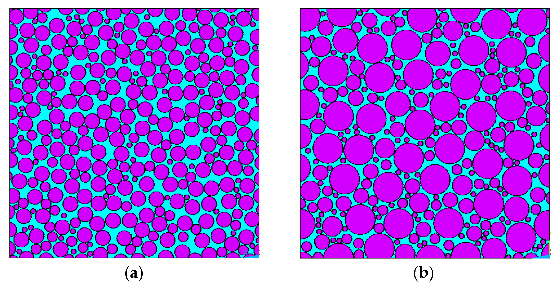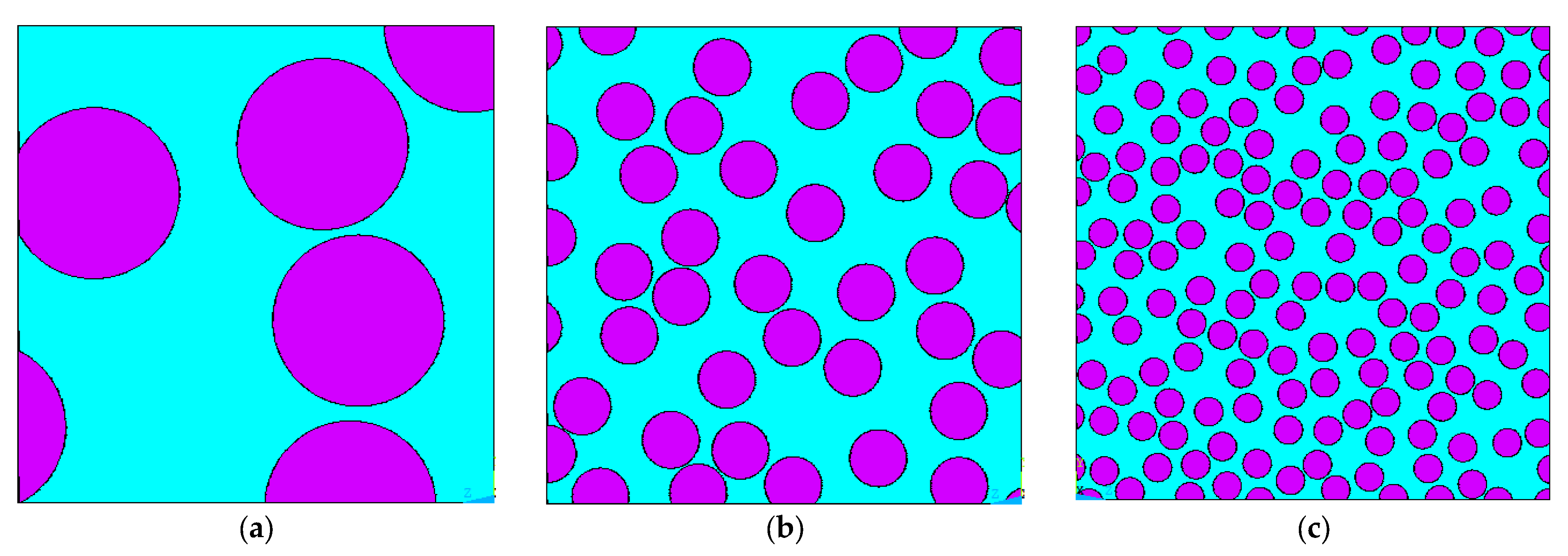Figure 2 shows two examples of the generated RVEs with different fiber radius profiles.

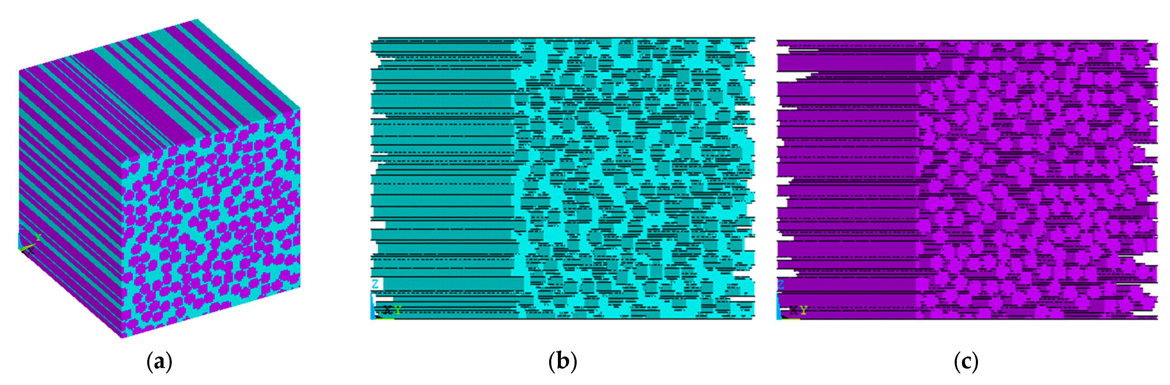
Based on the fiber coordinates and radii generated in MATLAB (R2023a), FEM modeling is performed using ANSYS APDL (2022 R2, ANSYS, Inc., Canonsburg, PA, USA). The fiber material is modeled as glass, with a Young’s modulus of 73.1 GPa and a Poisson’s ratio of 0.22, while the matrix material is epoxy, with a Young’s modulus of 3.45 GPa and a Poisson’s ratio of 0.35. A uniform voxel-based mesh is created using eight-node brick elements, initially assigning matrix properties to all elements. Based on the known coordinates and radii of all fibers, each voxel is then reassigned either the fiber or matrix material property depending on its location. A 2D view of the meshed RVE before and after fiber material assignment is shown in Figure 3, and the 3D view is presented in Figure 4.

3.2. Boundary Conditions for Charactirzing Unidirectional Lamina’s Effective Properties

Boundary conditions are applied following the work in [44] and summarized in

Table 2. Boundary conditions [44].

RVE Surface	$\mathbf{Young}’\mathbf{s} \mathbf{Modulus} ({\mathbf{E}}_{\mathbf{i}}$$) \mathbf{and} \mathbf{Poisson}’\mathbf{s} \mathbf{Ratio} ({\mathsf{\upsilon }}_{\mathbf{ij}}$)			$\mathbf{Shear} \mathbf{Modulus} ({\mathbf{G}}_{\mathbf{i}\mathbf{j}}$)
	${\mathbf{E}}_{\mathbf{x}},{\mathsf{\upsilon }}_{\mathbf{xy}},{\mathsf{\upsilon }}_{\mathbf{xz}}$	${\mathbf{E}}_{\mathbf{y}},{\mathsf{\upsilon }}_{\mathbf{yx}},{\mathsf{\upsilon }}_{\mathbf{yz}}$	${\mathbf{E}}_{\mathbf{z}},{\mathsf{\upsilon }}_{\mathbf{zx}},{\mathsf{\upsilon }}_{\mathbf{zy}}$	${\mathbf{G}}_{\mathbf{x}\mathbf{y}}$	${\mathbf{G}}_{\mathbf{y}\mathbf{z}}$	${\mathbf{G}}_{\mathbf{z}\mathbf{x}}$
x = 0	${\mathrm{u}}_{\mathrm{x}}=0$	${\mathrm{u}}_{\mathrm{x}}=0$	${\mathrm{u}}_{\mathrm{x}}=0$	${\mathrm{u}}_{\mathrm{x}}={\mathrm{u}}_{\mathrm{y}}={\mathrm{u}}_{\mathrm{z}}=0$	Free	Free
y = 0	${\mathrm{u}}_{\mathrm{y}}=0$	${\mathrm{u}}_{\mathrm{y}}=0$	${\mathrm{u}}_{\mathrm{y}}=0$	Free	${\mathrm{u}}_{\mathrm{x}}={\mathrm{u}}_{\mathrm{y}}={\mathrm{u}}_{\mathrm{z}}=0$	Free
z = 0	${\mathrm{u}}_{\mathrm{z}}=0$	${\mathrm{u}}_{\mathrm{z}}=0$	${\mathrm{u}}_{\mathrm{z}}=0$	Free	Free	${\mathrm{u}}_{\mathrm{x}}={\mathrm{u}}_{\mathrm{y}}={\mathrm{u}}_{\mathrm{z}}=0$
x = 100	${\mathrm{u}}_{\mathrm{x}}=1$	$$\begin{gathered} {\mathrm{u}}_{\mathrm{x}} (\mathrm{coupled} \\ \mathrm{DOFs}) \end{gathered}$$	$$\begin{gathered} {\mathrm{u}}_{\mathrm{x}} (\mathrm{coupled} \\ \mathrm{DOFs}) \end{gathered}$$	$$\begin{gathered} {\mathrm{u}}_{\mathrm{y}}=1,{\mathrm{u}}_{\mathrm{x}} \\ (\mathrm{coupled} \mathrm{DOFs}) \end{gathered}$$	Free	Free
y = 100	$$\begin{gathered} {\mathrm{u}}_{\mathrm{y}} (\mathrm{coupled} \\ \mathrm{DOFs}) \end{gathered}$$	${\mathrm{u}}_{\mathrm{y}}=1$	$$\begin{gathered} {\mathrm{u}}_{\mathrm{y}} (\mathrm{coupled} \\ \mathrm{DOFs}) \end{gathered}$$	Free	$$\begin{gathered} {\mathrm{u}}_{\mathrm{z}}=1,{\mathrm{u}}_{\mathrm{y}} \\ (\mathrm{coupled} \mathrm{DOFs}) \end{gathered}$$	Free
z = 100	$$\begin{gathered} {\mathrm{u}}_{\mathrm{x}} (\mathrm{coupled} \\ \mathrm{DOFs}) \end{gathered}$$	$$\begin{gathered} {\mathrm{u}}_{\mathrm{x}} (\mathrm{coupled} \\ \mathrm{DOFs}) \end{gathered}$$	${\mathrm{u}}_{\mathrm{z}}=1$	Free	Free	$$\begin{gathered} {\mathrm{u}}_{\mathrm{x}}=1,{\mathrm{u}}_{\mathrm{z}} \\ (\mathrm{coupled} \mathrm{DOFs}) \end{gathered}$$

, to predict Young’s modulus (${\mathrm{E}}_{\mathrm{i}}$), Poisson’s ratio (${\mathsf{\upsilon }}_{\mathrm{ij}}$), and shear modulus (${\mathrm{G}}_{\mathrm{ij}}$), along the three axial directions ($\mathrm{i},\mathrm{j}=\mathrm{x},\mathrm{y},\mathrm{z}$), where the origin of the coordinate system is placed at one vertex of the RVE, with the three coordinate axes along the adjacent edges. The length of the RVE is set to 100 units. For surfaces where coupled degrees of freedom (DOFs) are specified, the displacement in the corresponding direction is constrained to be identical.

In this study, periodic boundary conditions are not applied because uniform displacement constraints are enforced across opposing faces of the RVE, effectively eliminating boundary-induced artifacts. While the RVE geometry may not appear periodic (e.g., with non-complementary inclusions at boundaries), the displacement coupling ensures an average uniform strain field, which is sufficient to extract effective elastic properties under first-order homogenization principles. This approach is consistent with that of Luo [45], where periodicity was not imposed geometrically but was shown to be unnecessary under displacement-driven boundary conditions commonly adopted in numerical homogenization frameworks.

3.3. Calculation of Effective Properties of Unidirectional Lamina

After solving the finite element equations for nodal displacements, the elastic properties of the RVE such as Young’s modulus, Poisson’s ratio, and shear modulus are calculated using Equations (92)–(95).

$${\mathrm{E}}_{\mathrm{i}}={\displaystyle \frac{\overline{{\mathsf{\sigma }}_{\mathrm{i}}}}{\overline{{\mathsf{\epsilon }}_{\mathrm{i}}}}}, (\mathrm{i}=\mathrm{x},\mathrm{y},\mathrm{z})$$

(92)

$${\mathsf{\upsilon }}_{\mathrm{i}\mathrm{j}}=-{\displaystyle \frac{\overline{{\mathsf{\epsilon }}_{\mathrm{j}}}}{\overline{{\mathsf{\epsilon }}_{\mathrm{i}}}}}, (\mathrm{i},\mathrm{j}=\mathrm{x},\mathrm{y},\mathrm{z})$$

(93)

$${\mathrm{G}}_{\mathrm{i}\mathrm{j}}=-{\displaystyle \frac{\overline{{\mathsf{\tau }}_{\mathrm{i}\mathrm{j}}}}{\overline{{\mathsf{\gamma }}_{\mathrm{i}\mathrm{j}}}}}, (\mathrm{i},\mathrm{j}=\mathrm{x},\mathrm{y},\mathrm{z})$$

(94)

$$\overline{{\mathsf{\sigma }}_{\mathrm{i}}}={\int }_{\mathrm{V}}{\mathsf{\sigma }}_{\mathrm{i}}\mathrm{d}\mathrm{V}, \overline{{\mathsf{\epsilon }}_{\mathrm{i}}}={\int }_{\mathrm{V}}{\mathsf{\epsilon }}_{\mathrm{i}}\mathrm{d}\mathrm{V}, \overline{{\mathsf{\tau }}_{\mathrm{i}\mathrm{j}}}={\int }_{\mathrm{V}}{\mathsf{\tau }}_{\mathrm{i}\mathrm{j}}\mathrm{d}\mathrm{V}, \overline{{\mathsf{\gamma }}_{\mathrm{i}\mathrm{j}}}={\int }_{\mathrm{V}}{\mathsf{\gamma }}_{\mathrm{i}\mathrm{j}}\mathrm{d}\mathrm{V}$$

(95)

Here, ${\mathsf{\sigma }}_{\mathrm{i}}$, ${\mathsf{\epsilon }}_{\mathrm{i}}$, ${\mathsf{\tau }}_{\mathrm{ij}},$ ${\mathsf{\gamma }}_{\mathrm{ij}}$, and $\mathrm{V}$ are normal stress, normal strain, shear stress, shear strain and volume of the RVE, respectively.

3.4. Creation of Laminate Plate/Shell RVE

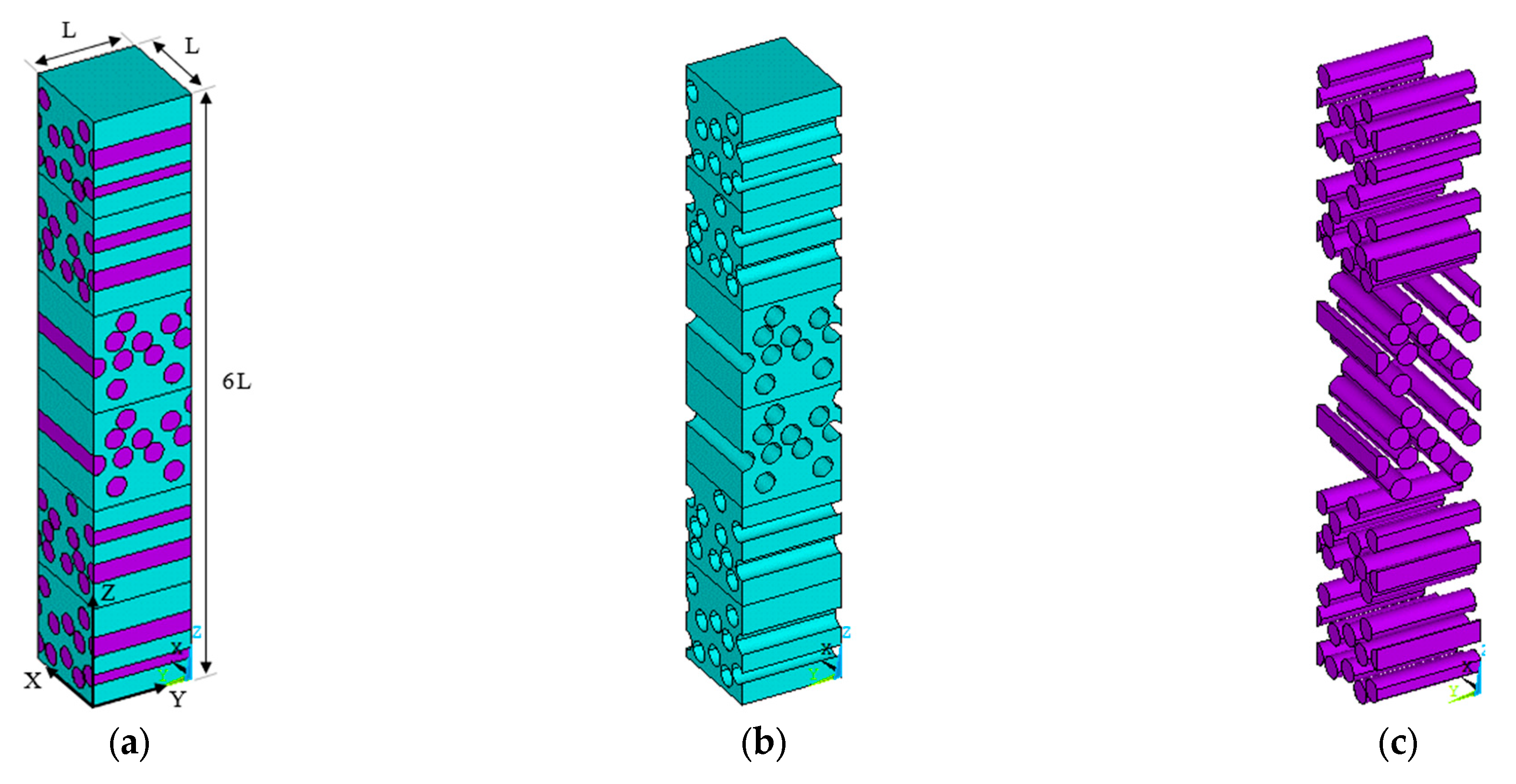
A six-layer symmetric laminate with a [90/90/0/0/90/90] stacking sequence is modeled. The laminate consists of three distinct unidirectional fiber layers, each having a different random distribution of fibers to capture the natural variability in fiber placement. Although the fiber distributions differ, the fiber volume fraction for each layer is closely controlled to remain nearly identical, with variations kept within approximately 1%. To maintain laminate symmetry, the remaining three layers are created by mirroring the initial three layers.

The fiber centers were generated using the same MATLAB code described in the previous section. For the laminate, an additional constraint was introduced: fibers were restricted to remain within the top and bottom boundaries of each layer, corresponding to the layer thickness, but were allowed to pass through the left and right boundaries, reflecting the material continuity along the length and width directions of the laminate.

The overall laminate was assembled by stacking the generated layers together, forming a composite structure with dimensions of 100 × 100 × 600 units. This approach to constructing a laminate by stacking distinct layers was previously adopted by Song et al. [46]. The resulting RVE and its coordinate system are shown in Figure 5.

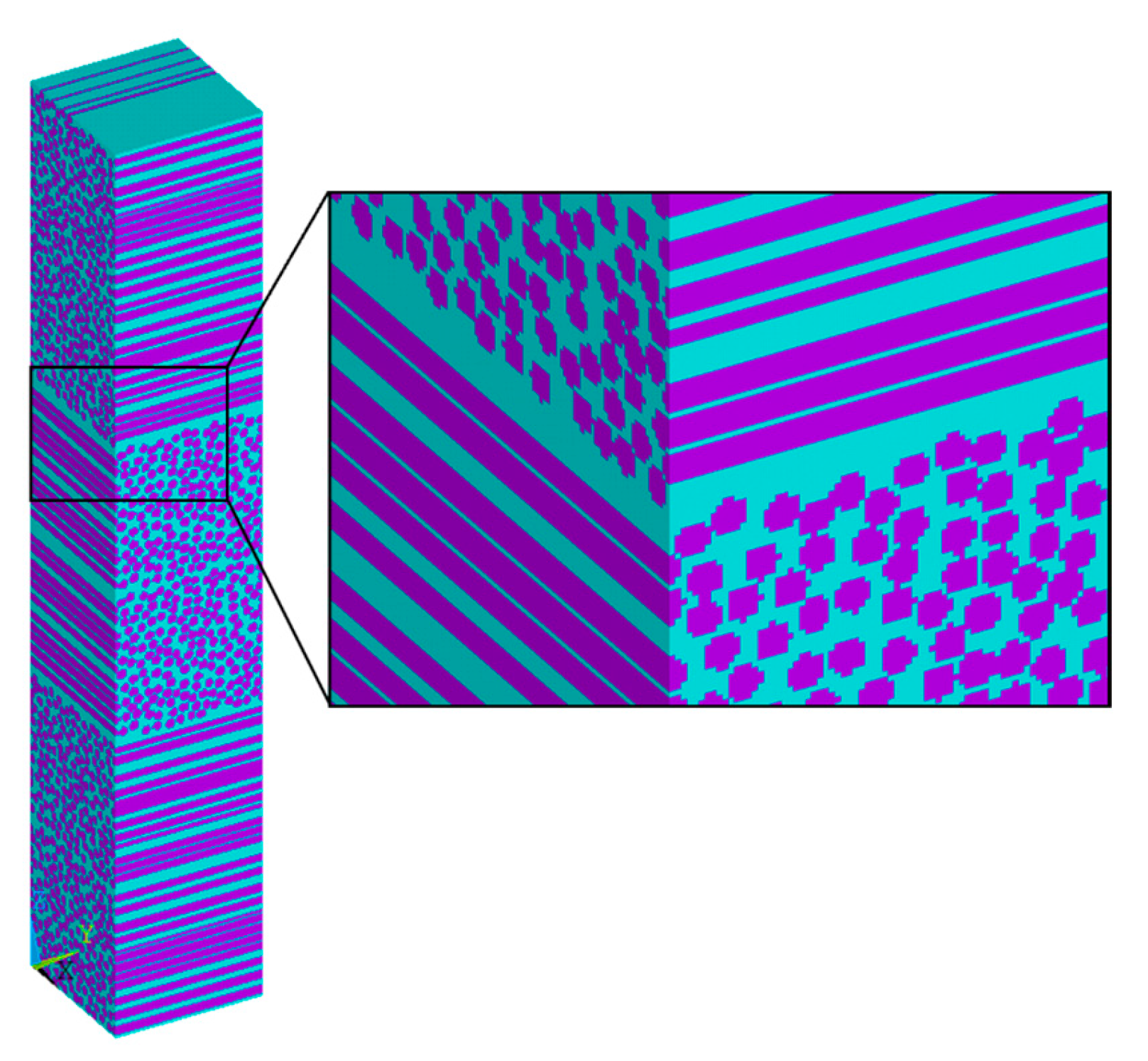
To generate the laminate model, the same materials and procedures used for unidirectional composites are applied, with the additional considerations described earlier. Each layer is then meshed uniformly one by one. During meshing, a local coordinate system is assigned to each layer based on its fiber orientation relative to the global coordinate system, ensuring that the correct material properties are later assigned. Elements located within the fiber regions are identified based on the fiber center positions and assigned the fiber material. Figure 6 shows the meshed RVE, with the matrix and fiber phases displayed separately in Figure 7.

3.5. Boundary Conditions for Characterizing Laminate Plate/Shell Effective Properties

To determine the in-plane stiffness matrix (A) and out-of-plane shear stiffness matrix (H), the in-plane elastic constants (${\mathrm{E}}_{\mathrm{x}}$, ${\mathrm{E}}_{\mathrm{y}}$, ${\mathsf{\upsilon }}_{\mathrm{xy}}$, and ${\mathrm{G}}_{\mathrm{x}\mathrm{y}}$), the bending elastic constants (${\mathrm{E}}_x^f$, ${\mathrm{E}}_y^f$, ${\mathrm{G}}_{xy}^f$, and ${\mathsf{\upsilon }}_{xy}^f$), and the out-of-plane shear constants (${\mathrm{G}}_{\mathrm{x}\mathrm{z}}$ and ${\mathrm{G}}_{\mathrm{y}\mathrm{z}}$) are computed using the boundary conditions summarized in Table 3. For computational efficiency, and because the laminate is symmetric, only half of the laminate layers are modeled. The boundary conditions listed in Table 3 correspond to this reduced model.

Table 3. Boundary conditions for characterizing laminate effective properties.

RVE Surface	In-Plane Modulus			Bending Modulus			Shear Modulus
	${\mathrm{E}}_{\mathrm{x}},{\mathsf{\upsilon }}_{\mathrm{xy}}$	${\mathrm{E}}_{\mathrm{y}}$	${\mathrm{G}}_{\mathrm{x}\mathrm{y}}$	${\mathrm{E}}_{\mathrm{x}}^{\mathrm{f}},{\mathsf{\upsilon }}_{\mathrm{x}\mathrm{y}}^{\mathrm{f}}$	${\mathrm{E}}_{\mathrm{y}}^{\mathrm{f}}$	${\mathrm{G}}_{\mathrm{x}\mathrm{y}}^{\mathrm{f}}$	${\mathrm{G}}_{\mathrm{y}\mathrm{z}}$	${\mathrm{G}}_{\mathrm{x}\mathrm{z}}$
x = 300	${\mathrm{u}}_{\mathrm{x}}=0$	${\mathrm{u}}_{\mathrm{x}}=0$	${\mathrm{u}}_{\mathrm{x}}={\mathrm{u}}_{\mathrm{y}}=0$	${\mathrm{u}}_{\mathrm{x}}=0$	${\mathrm{u}}_{\mathrm{x}}=0$	${\mathrm{u}}_{\mathrm{x}}={\mathrm{u}}_{\mathrm{y}}={\mathrm{u}}_{\mathrm{z}}=0$	$$\begin{gathered} {\mathrm{u}}_{\mathrm{x}} (\mathrm{coupled} \\ \mathrm{DOFs}) \end{gathered}$$	${\mathrm{u}}_{\mathrm{y}}={\displaystyle \frac{\mathrm{z}}{3\mathrm{L}}}$
y = 300	${\mathrm{u}}_{\mathrm{y}}=0$	${\mathrm{u}}_{\mathrm{y}}=0$	${\mathrm{u}}_{\mathrm{y}}={\displaystyle \frac{\mathrm{x}}{\mathrm{L}}}$	${\mathrm{u}}_{\mathrm{y}}=0$	${\mathrm{u}}_{\mathrm{y}}=0$	Free	${\mathrm{u}}_{\mathrm{y}}={\displaystyle \frac{\mathrm{z}}{3\mathrm{L}}}$	$$\begin{gathered} {\mathrm{u}}_{\mathrm{y}} (\mathrm{coupled} \\ \mathrm{DOFs}) \end{gathered}$$
z = 300	${\mathrm{u}}_{\mathrm{z}}=0$	${\mathrm{u}}_{\mathrm{z}}=0$	${\mathrm{u}}_{\mathrm{z}}=0$	${\mathrm{u}}_{\mathrm{z}}=0$	${\mathrm{u}}_{\mathrm{z}}=0$	Free	${\mathrm{u}}_{\mathrm{x}}={\mathrm{u}}_{\mathrm{y}}={\mathrm{u}}_{\mathrm{z}}=0$	${\mathrm{u}}_{\mathrm{x}}={\mathrm{u}}_{\mathrm{y}}={\mathrm{u}}_{\mathrm{z}}=0$
x = 0	${\mathrm{u}}_{\mathrm{x}}=1$	$$\begin{gathered} {\mathrm{u}}_{\mathrm{x}} (\mathrm{coupled} \\ \mathrm{DOFs}) \end{gathered}$$	${\mathrm{u}}_{\mathrm{y}}=1,$ $$\begin{gathered} {\mathrm{u}}_{\mathrm{x}} (\mathrm{coupled} \\ \mathrm{DOFs}) \end{gathered}$$	${\mathrm{u}}_{\mathrm{x}}=-{\displaystyle \frac{\mathrm{z}}{3\mathrm{L}}}$	Figure 8	$$\begin{gathered} {\mathrm{u}}_{\mathrm{x}}=0 \\ {\mathrm{u}}_{\mathrm{y}}=-{\displaystyle \frac{\mathrm{z}}{6\mathrm{L}}}+0.5 \\ {\mathrm{u}}_{\mathrm{z}}={\displaystyle \frac{\mathrm{y}}{6\mathrm{L}}}-0.5 \end{gathered}$$	$$\begin{gathered} {\mathrm{u}}_{\mathrm{x}} (\mathrm{coupled} \\ \mathrm{DOFs}) \end{gathered}$$	${\mathrm{u}}_{\mathrm{y}}={\displaystyle \frac{\mathrm{z}}{3\mathrm{L}}}$
y = 0	$$\begin{gathered} {\mathrm{u}}_{\mathrm{y}} (\mathrm{coupled} \\ \mathrm{DOFs}) \end{gathered}$$	${\mathrm{u}}_{\mathrm{y}}=1$	${\mathrm{u}}_{\mathrm{y}}={\displaystyle \frac{\mathrm{x}}{\mathrm{L}}}$	Figure 8	${\mathrm{u}}_{\mathrm{y}}=-{\displaystyle \frac{\mathrm{z}}{3\mathrm{L}}}$	Free	${\mathrm{u}}_{\mathrm{y}}={\displaystyle \frac{\mathrm{z}}{3\mathrm{L}}}$	$$\begin{gathered} {\mathrm{u}}_{\mathrm{y}} (\mathrm{coupled} \\ \mathrm{DOFs}) \end{gathered}$$
z = 0	Free	Free	Free	Free	Free	Free	$$\begin{gathered} {\mathrm{u}}_{\mathrm{y}}=1,{\mathrm{u}}_{\mathrm{z}} \\ (\mathrm{coupled} \mathrm{DOFs}) \end{gathered}$$	$$\begin{gathered} {\mathrm{u}}_{\mathrm{x}}=1,{\mathrm{u}}_{\mathrm{z}} \\ (\mathrm{coupled} \mathrm{DOFs}) \end{gathered}$$

Table 3. Boundary conditions for characterizing laminate effective properties.

RVE Surface	In-Plane Modulus			Bending Modulus			Shear Modulus
	${\mathrm{E}}_{\mathrm{x}},{\mathsf{\upsilon }}_{\mathrm{xy}}$	${\mathrm{E}}_{\mathrm{y}}$	${\mathrm{G}}_{\mathrm{x}\mathrm{y}}$	${\mathrm{E}}_{\mathrm{x}}^{\mathrm{f}},{\mathsf{\upsilon }}_{\mathrm{x}\mathrm{y}}^{\mathrm{f}}$	${\mathrm{E}}_{\mathrm{y}}^{\mathrm{f}}$	${\mathrm{G}}_{\mathrm{x}\mathrm{y}}^{\mathrm{f}}$	${\mathrm{G}}_{\mathrm{y}\mathrm{z}}$	${\mathrm{G}}_{\mathrm{x}\mathrm{z}}$
x = 300	${\mathrm{u}}_{\mathrm{x}}=0$	${\mathrm{u}}_{\mathrm{x}}=0$	${\mathrm{u}}_{\mathrm{x}}={\mathrm{u}}_{\mathrm{y}}=0$	${\mathrm{u}}_{\mathrm{x}}=0$	${\mathrm{u}}_{\mathrm{x}}=0$	${\mathrm{u}}_{\mathrm{x}}={\mathrm{u}}_{\mathrm{y}}={\mathrm{u}}_{\mathrm{z}}=0$	$$\begin{gathered} {\mathrm{u}}_{\mathrm{x}} (\mathrm{coupled} \\ \mathrm{DOFs}) \end{gathered}$$	${\mathrm{u}}_{\mathrm{y}}={\displaystyle \frac{\mathrm{z}}{3\mathrm{L}}}$
y = 300	${\mathrm{u}}_{\mathrm{y}}=0$	${\mathrm{u}}_{\mathrm{y}}=0$	${\mathrm{u}}_{\mathrm{y}}={\displaystyle \frac{\mathrm{x}}{\mathrm{L}}}$	${\mathrm{u}}_{\mathrm{y}}=0$	${\mathrm{u}}_{\mathrm{y}}=0$	Free	${\mathrm{u}}_{\mathrm{y}}={\displaystyle \frac{\mathrm{z}}{3\mathrm{L}}}$	$$\begin{gathered} {\mathrm{u}}_{\mathrm{y}} (\mathrm{coupled} \\ \mathrm{DOFs}) \end{gathered}$$
z = 300	${\mathrm{u}}_{\mathrm{z}}=0$	${\mathrm{u}}_{\mathrm{z}}=0$	${\mathrm{u}}_{\mathrm{z}}=0$	${\mathrm{u}}_{\mathrm{z}}=0$	${\mathrm{u}}_{\mathrm{z}}=0$	Free	${\mathrm{u}}_{\mathrm{x}}={\mathrm{u}}_{\mathrm{y}}={\mathrm{u}}_{\mathrm{z}}=0$	${\mathrm{u}}_{\mathrm{x}}={\mathrm{u}}_{\mathrm{y}}={\mathrm{u}}_{\mathrm{z}}=0$
x = 0	${\mathrm{u}}_{\mathrm{x}}=1$	$$\begin{gathered} {\mathrm{u}}_{\mathrm{x}} (\mathrm{coupled} \\ \mathrm{DOFs}) \end{gathered}$$	${\mathrm{u}}_{\mathrm{y}}=1,$ $$\begin{gathered} {\mathrm{u}}_{\mathrm{x}} (\mathrm{coupled} \\ \mathrm{DOFs}) \end{gathered}$$	${\mathrm{u}}_{\mathrm{x}}=-{\displaystyle \frac{\mathrm{z}}{3\mathrm{L}}}$	Figure 8	$$\begin{gathered} {\mathrm{u}}_{\mathrm{x}}=0 \\ {\mathrm{u}}_{\mathrm{y}}=-{\displaystyle \frac{\mathrm{z}}{6\mathrm{L}}}+0.5 \\ {\mathrm{u}}_{\mathrm{z}}={\displaystyle \frac{\mathrm{y}}{6\mathrm{L}}}-0.5 \end{gathered}$$	$$\begin{gathered} {\mathrm{u}}_{\mathrm{x}} (\mathrm{coupled} \\ \mathrm{DOFs}) \end{gathered}$$	${\mathrm{u}}_{\mathrm{y}}={\displaystyle \frac{\mathrm{z}}{3\mathrm{L}}}$
y = 0	$$\begin{gathered} {\mathrm{u}}_{\mathrm{y}} (\mathrm{coupled} \\ \mathrm{DOFs}) \end{gathered}$$	${\mathrm{u}}_{\mathrm{y}}=1$	${\mathrm{u}}_{\mathrm{y}}={\displaystyle \frac{\mathrm{x}}{\mathrm{L}}}$	Figure 8	${\mathrm{u}}_{\mathrm{y}}=-{\displaystyle \frac{\mathrm{z}}{3\mathrm{L}}}$	Free	${\mathrm{u}}_{\mathrm{y}}={\displaystyle \frac{\mathrm{z}}{3\mathrm{L}}}$	$$\begin{gathered} {\mathrm{u}}_{\mathrm{y}} (\mathrm{coupled} \\ \mathrm{DOFs}) \end{gathered}$$
z = 0	Free	Free	Free	Free	Free	Free	$$\begin{gathered} {\mathrm{u}}_{\mathrm{y}}=1,{\mathrm{u}}_{\mathrm{z}} \\ (\mathrm{coupled} \mathrm{DOFs}) \end{gathered}$$	$$\begin{gathered} {\mathrm{u}}_{\mathrm{x}}=1,{\mathrm{u}}_{\mathrm{z}} \\ (\mathrm{coupled} \mathrm{DOFs}) \end{gathered}$$

Figure 8. Displacement boundary conditions applied to preserve the planarity of a surface before and after deformation. The two views, (a,b), illustrate the same boundary setup from different perspectives.

Figure 8. Displacement boundary conditions applied to preserve the planarity of a surface before and after deformation. The two views, (a,b), illustrate the same boundary setup from different perspectives.

3.6. Calculation of Laminate Plate/Shell Effective Properties

The elements of the A, D and H matrices are then extracted using Equations (96)–(105), which are modified forms of Equations (10)–(19).

$${\mathrm{A}}_{11}={\displaystyle \frac{\mathrm{t}{\mathrm{E}}_{\mathrm{x}\mathrm{x}}^2}{{\mathrm{E}}_{\mathrm{x}\mathrm{x}}-{\mathsf{\nu }}_{\mathrm{x}\mathrm{y}}^2{\mathrm{E}}_{\mathrm{y}\mathrm{y}}}}$$

(96)

$${\mathrm{A}}_{22}={\displaystyle \frac{\mathrm{t}{\mathrm{E}}_{\mathrm{x}\mathrm{x}}{\mathrm{E}}_{\mathrm{y}\mathrm{y}}}{{\mathrm{E}}_{\mathrm{x}\mathrm{x}}-{\mathsf{\nu }}_{\mathrm{x}\mathrm{y}}^2{\mathrm{E}}_{\mathrm{y}\mathrm{y}}}}$$

(97)

$${\mathrm{A}}_{12}={\mathsf{\nu }}_{\mathrm{x}\mathrm{y}}{\mathrm{A}}_{22}$$

(98)

$${\mathrm{A}}_{33}=\mathrm{t} {\mathrm{G}}_{\mathrm{x}\mathrm{y}}$$

(99)

$${\mathrm{D}}_{11}={\displaystyle \frac{{\mathrm{t}}^3{\mathrm{E}}_{\mathrm{x}\mathrm{x}}^2}{{\mathrm{E}}_{\mathrm{x}\mathrm{x}}-{\mathsf{\nu }}_{\mathrm{x}\mathrm{y}}^2{\mathrm{E}}_{\mathrm{y}\mathrm{y}}}}$$

(100)

$${\mathrm{D}}_{22}={\displaystyle \frac{{\mathrm{t}}^3{\mathrm{E}}_{\mathrm{x}\mathrm{x}}{\mathrm{E}}_{\mathrm{y}\mathrm{y}}}{{\mathrm{E}}_{\mathrm{x}\mathrm{x}}-{\mathsf{\nu }}_{\mathrm{x}\mathrm{y}}^2{\mathrm{E}}_{\mathrm{y}\mathrm{y}}}}$$

(101)

$${\mathrm{D}}_{12}={\mathsf{\nu }}_{\mathrm{x}\mathrm{y}}{\mathrm{D}}_{22}$$

(102)

$${\mathrm{D}}_{33}={\mathrm{t}}^3{\mathrm{G}}_{\mathrm{x}\mathrm{y}}$$

(103)

$${\mathrm{H}}_{11}=\mathrm{t} {\mathrm{G}}_{\mathrm{y}\mathrm{z}}$$

(104)

$${\mathrm{H}}_{22}=\mathrm{t} {\mathrm{G}}_{\mathrm{x}\mathrm{z}}$$

(105)

4. Results

This section presents the results of the numerical simulations and micromechanical model predictions. The results are organized into two parts: unidirectional lamina effective properties and laminate plate/shell effective properties. First, the influence of fiber aspect ratio on the transverse elastic properties of unidirectional composites is presented. Then, the accuracy of various micromechanical models is assessed by comparing their predictions against voxel-based finite element modeling (VB-FEM) results and available experimental data. For laminates, appropriate micromechanics models are selected, and the predicted stiffness matrices are compared with numerical and experimental results. This comprehensive evaluation highlights the strengths and limitations of different modeling approaches for predicting composite stiffness properties.

4.1. Unidirectional Lamina Effective Properties

This section presents the effect of the fiber length-to-diameter ratio on the elastic properties of composites and identifies an appropriate fiber size for subsequent modeling. The VB-FEM predictions are then compared with several micromechanical models, including VR, Chamis, HT, HTm, GSC, MT, Bridging, and two iterative isotropized models (Iter-Iso-VR and Iter-Iso-HS), using both simulation and experimental data.

4.1.1. Effect of Fiber Length-to-Diameter Ratio on Transverse Properties

Different fiber diameters are modeled while maintaining a fixed fiber volume fraction of 40%. For each fiber diameter, four randomly generated RVEs are averaged to obtain more reliable results. To reduce the influence of microstructural variability and ensure statistical relevance, four distinct RVEs were generated and simulated for each fiber diameter. Each RVE, including those shown in Figure 9, contained several hundred non-overlapping fibers and was used in full finite element simulations. The effective elastic properties were obtained by averaging the results across the four RVEs for each configuration.

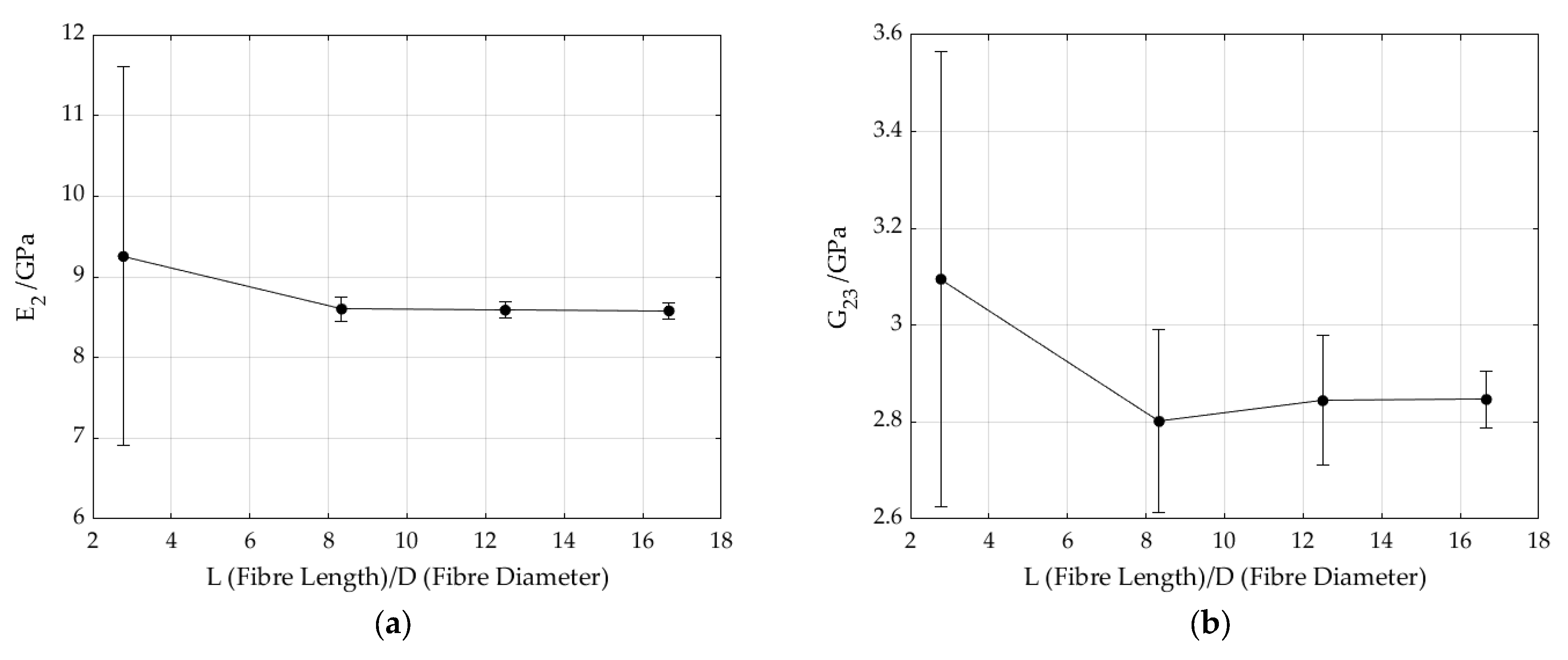
Figure 10 shows the effect of fiber aspect ratio on the transverse Young’s modulus and transverse shear modulus of a glass–epoxy composite at a fixed fiber volume fraction of 40%, demonstrating that increasing the fiber aspect ratio reduces the variability of the predicted properties without significantly affecting their average values.

The figure illustrates that as the fiber aspect ratio exceeds 8, the variance in the results decreases, while the mean modulus values remain relatively stable. This stabilization effect is more pronounced for the transverse shear modulus than for the transverse Young’s modulus. To minimize result variability, fibers with an aspect ratio of 16.67, corresponding to a fiber radius of 3 units in an RVE of 100 units, are used in the main simulations. For cases requiring volume fractions greater than 60%, fibers with a maximum radius of six units, corresponding to an aspect ratio of 8.33, are used in this study.

4.1.2. Comparison of Micromechanics Model Predictions with VB-FEM and Experimental Results

This section compares the performance of the selected micromechanics models—Voigt–Reuss (VR), Chamis, Halpin–Tsai (HT), Modified Halpin–Tsai (HTm), Generalized Self-Consistent (GSC), Mori–Tanaka (MT), the Bridging Model (Br), the Iterative Isotropized Voigt–Reuss bounds (Iter-Iso-VR), and the Iterative Isotropized Hashin–Shtrikman bounds (Iter-Iso-HS)—in predicting the elastic properties of glass–epoxy unidirectional composites. The Iter-Iso-VR and Iter-Iso-HS models are applied specifically for predicting the transverse properties. The VB-FEM simulation results and the experimental data from [47] are used as references for the comparison. It is important to note that among the five elastic constants considered, ${\mathrm{E}}_1$ can be accurately predicted by most micromechanics models, as reported by Younes et al. [47]. Of the remaining constants, only the transverse Young’s modulus ${\mathrm{E}}_2$ has corresponding experimental data available in the literature. For the others—${\mathrm{G}}_{12}$, ${\mathrm{G}}_{23}$, and ${\mathrm{G}}_{23}$—no experimental measurements were found. Therefore, voxel-based FEM results, which have been validated in previous studies [16,33,44,45] and are recognized for their accuracy in predicting effective properties, are used as the reference for evaluating the micromechanics models.

The following observations are drawn from the comparisons presented in Figure 11.

• Young’s moduli E₁ and E₂

For the longitudinal Young’s modulus (E₁), all micromechanics models exhibit consistently high accuracy, closely matching the VB-FEM results and demonstrating reliable predictive performance. In contrast, for the transverse Young’s modulus (E₂), while the VB-FEM and experimental results are generally close, the VB-FEM predictions are slightly higher. This discrepancy may be attributed to porosity in the experimental composites, which is not captured in the numerical simulations, as well as potential differences in boundary conditions between the experiments and the FEM models. At fiber volume fractions below 20%, all micromechanics models predict E₂ with good accuracy. However, as the fiber volume fraction increases, discrepancies among the models become more pronounced. Compared to experimental data, the Voigt–Reuss model tends to underestimate E₂, whereas the iterative models (Iter-Iso-VR and Iter-Iso-HS) overestimate it, with the other models falling between these bounds. Among them, the Chamis and HT models provide the closest agreement with experimental data.

When focusing on comparisons against VB-FEM results, the Bridging Model shows the highest accuracy, followed by the HT and Chamis models. Although the Bridging and HT models use empirical fitting parameters, their performance relative to VB-FEM remains strong. However, the HTm model becomes less accurate at fiber volume fractions greater than 60–70%.

2.

Shear moduli G₁₂ and G₂₃

No experimental data were available for the shear moduli in the mentioned reference. Based on the VB-FEM results, predictions for the longitudinal shear modulus (G₁₂) show that the Bridging (Br) Model provides the closest agreement with the VB-FEM results, while the Voigt–Reuss model exhibits the largest deviation. Similarly, for the out-of-plane shear modulus (G₂₃), the Bridging Model again shows the best alignment with the VB-FEM predictions. Considering that the Bridging Model relies on empirical fitting parameters, the next most accurate model relative to FEM results is the Chamis model.

3.

Poisson’s ratio v₁₂

For predicting the in-plane Poisson’s ratio (ν₁₂), the Mori–Tanaka (MT) and Generalized Self-Consistent (GSC) models show the closest agreement with the VB-FEM results at lower fiber volume fractions. However, as the volume fraction increases, the VB-FEM predictions begin to deviate from these models, yielding slightly lower values. This deviation may be attributed to fiber interactions and microstructural effects that become more pronounced at higher volume fractions and are not fully captured by the MT and GSC models.

4.2. Laminate Plate/Shell Effective Properties

This section reports the effective stiffness parameters of symmetric cross-ply laminate plates using both micromechanics-based analytical predictions and voxel-based finite element modeling (VB-FEM). The stiffness predictions from FSDT are computed analytically using homogenized lamina properties derived from micromechanics models. As a result, their accuracy strongly depends on the quality of the input properties—particularly the transverse modulus ${\mathrm{E}}_2$ and out-of-plane shear modulus ${\mathrm{G}}_{23}$. In contrast, VB-FEM simulates the actual microstructure of the laminate, capturing local interactions and variability directly. This allows VB-FEM to provide more accurate and reliable stiffness predictions, especially when complex microstructural effects are present. First, a subset of micromechanics models capable of predicting all five independent lamina properties (E₁, E₂, G₁₂, G₂₃, and ν₁₂) is selected for input into First-Order Shear Deformation Theory (FSDT). Using these models, the in-plane stiffness matrix (A) and the transverse shear stiffness matrix (H) of the laminate are computed. The predictions are then compared with VB-FEM results and available experimental data to assess the reliability of each micromechanics model in the context of laminate-level behavior.

4.2.1. Selection of Micromechanics Models for Laminate Stiffness Prediction

To accurately predict laminate stiffness, a micromechanics model must provide all five elastic properties of the lamina: E₁, E₂, G₁₂, G₂₃, and ν₁₂. All models demonstrated similar accuracy in predicting the longitudinal Young’s modulus (E₁) for glass–epoxy materials. For Poisson’s ratio (ν₁₂), GSCM and MT models provided predictions closer to numerical results, despite the lack of experimental data for validation. The HTm model showed poor accuracy in predicting E₂ at high fiber volume fractions, and while the original HT model was accurate for glass–epoxy, it lacked formulas for the out-of-plane shear modulus (G₂₃), which are crucial for laminate analysis.

Considering overall performance, GSCM and MT models are strong candidates due to their consistent accuracy across all properties. The Bridging Model shows the closest results with VB-FEM results for E₂, G₁₂, and G₂₃ in glass–epoxy and is selected for further analysis. However, its reliance on empirical parameters may reduce its robustness, especially when there is a large difference between the moduli of fiber and matrix phases [20]. Therefore, GSCM, MT, Chamis, and Bridging Models are selected for laminate stiffness prediction due to their ability to provide all five elastic properties with good accuracy. The simpler model of Voigt–Ruess may serve as a baseline reference but is generally less reliable for critical properties like E₂ and G₂₃.

4.2.2. Validation with Experimental Data

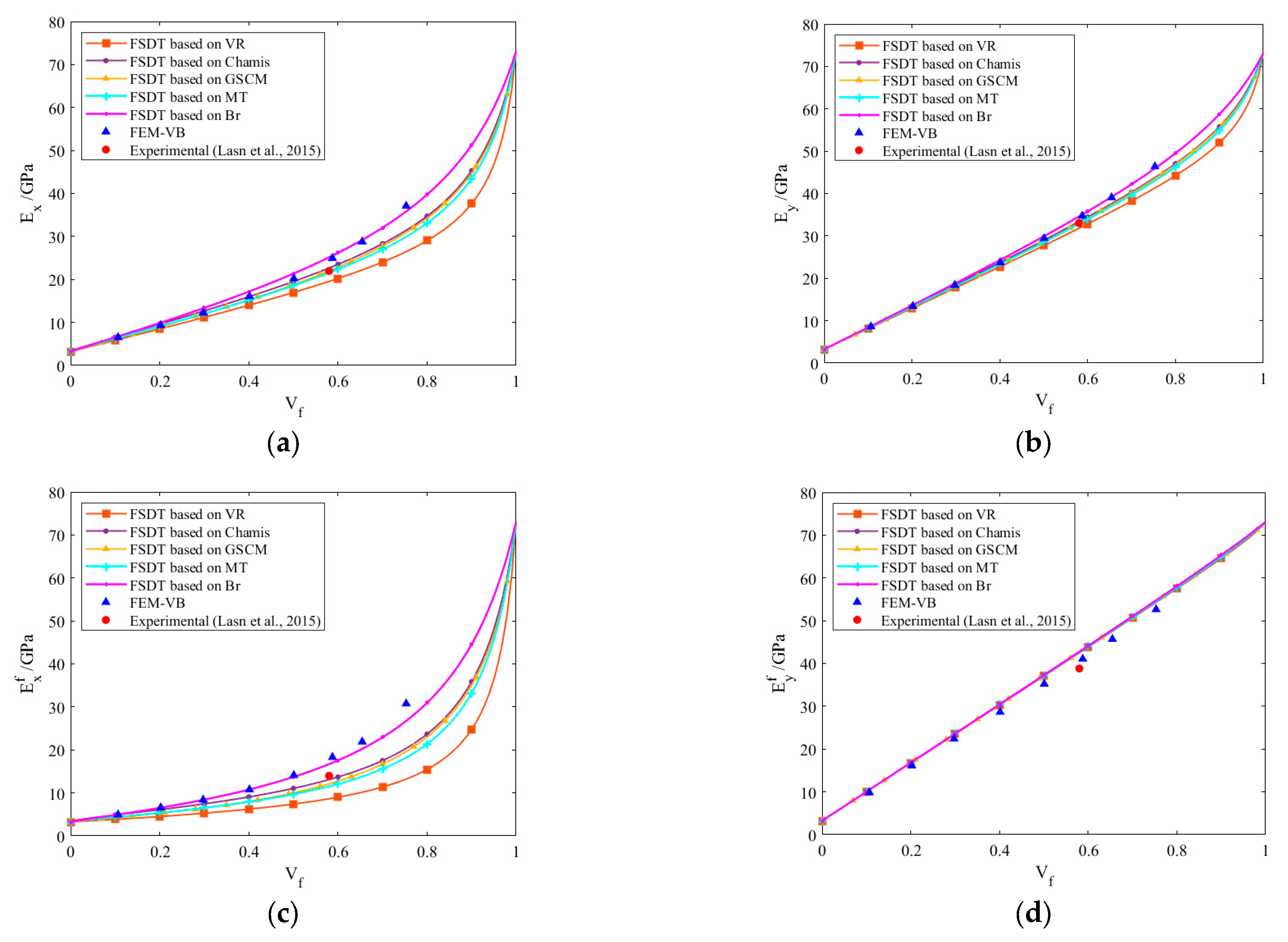
For laminates, experimental data is typically available only for Young’s moduli. To validate the finite element results, Figure 12 compares experimental, VB-FEM, and analytical predictions for E_x, E_y, ${\mathrm{E}}_{\mathrm{x}}^{\mathrm{f}}$, and ${\mathrm{E}}_{\mathrm{y}}^{\mathrm{f}}$, using experimental data reported by Lasn et al. [48].

The VB-FEM results are slightly higher than the experimental data, which may be attributed to the porosity present in the tested material. Since VB-FEM simulations typically assume fully dense, defect-free materials, they may overestimate stiffness relative to experimental measurements. Among the analytical models, the Bridging Model produces predictions that most closely align with the FEM results.

4.2.3. In-Plane Stiffness Matrix (A) Parameters

Figure 13 shows the non-zero and independent elements of the in-plane matrix (A) as predicted by FSDT using the selected micromechanics models, alongside the corresponding VB-FEM results.

The values of A(1,1) and A(2,2) depend on E_x, Ey, and ν_xy, with A(1,1) being more sensitive to E_x. Since E_x is influenced by the four 90° plies and two 0° plies, while E_γ is governed by the reverse stacking sequence, the higher accuracy in predicting the longitudinal modulus (E_γ) leads to better agreement for A(2,2) across all models. Overall, the Bridging Model provides the most accurate predictions for both A(1,1) and A(2,2), followed by the Chamis model, while the Voigt–Reuss model consistently underperforms.

For A(1,2), the FEM predictions up to a 40% fiber volume fraction closely match those from the Mori–Tanaka (MT) and Generalized Self-Consistent (GSC) models. As the volume fraction increases, the FEM values approach those predicted by the Bridging Model. This trend reflects earlier findings in unidirectional composites, where ν₁₂ predictions from MT and GSC aligned well with FEM, particularly at mid-range volume fractions. The trend observed for A(3,3) mirrors that of the shear modulus in unidirectional composites. The FEM results are slightly higher than the analytical predictions but remain closest to those from the Bridging Model.

4.2.4. Bending Stiffness Matrix (D) Parameters

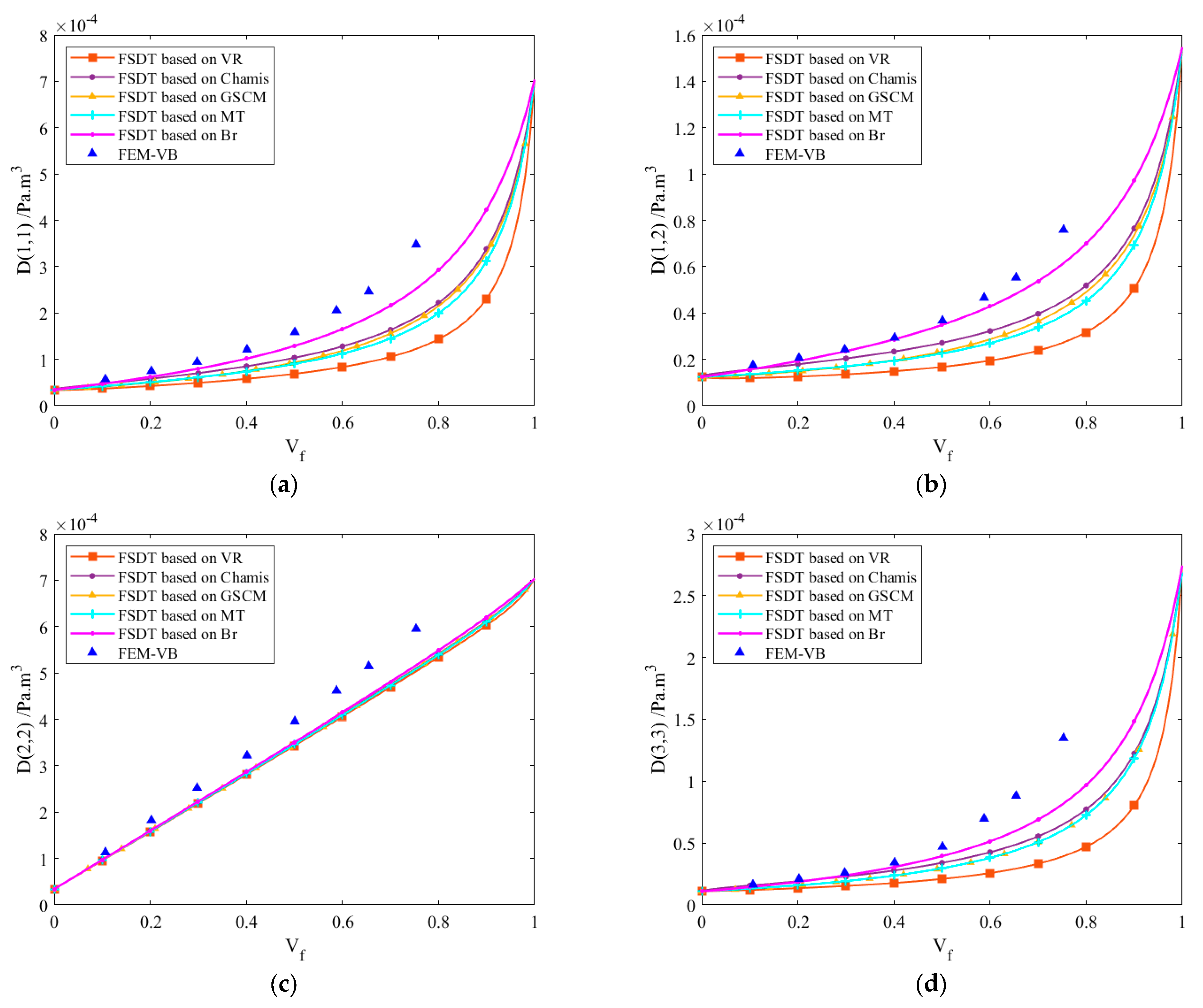
Figure 14 presents the non-zero and independent elements of the bending stiffness matrix (D) as predicted by First-Order Shear Deformation Theory (FSDT) using the selected micromechanics models, alongside corresponding results from VB-FEM.

The VB-FEM results for the bending stiffness matrix elements D(1,1), D(1,2), and D(2,2) are slightly higher than the corresponding predictions from the micromechanics-based models, even at a low fiber volume fraction of 0.1. Such discrepancies were not observed in the prediction of the in-plane stiffness matrix (A). The deviation originates from the estimation of Poisson’s ratio ${\mathsf{\upsilon }}_{\mathrm{x}\mathrm{y}}^{\mathrm{f}}$. During bending about the x-axis, efforts were made to constrain the plane at y = 100 to remain flat; however, residual warping deformation was observed, indicating incomplete constraint enforcement. This directly affected the computed value of ${\mathsf{\upsilon }}_{\mathrm{x}\mathrm{y}}^{\mathrm{f}}$, which in turn influenced the accuracy of D(1,1), D(1,2), and D(2,2), while leaving D(3,3) unaffected.

Among these, D(2,2) is more sensitive to ${\mathrm{E}}_y^f$, which is primarily influenced by the stiffness of the 0° plies located at the outermost layers of the laminate during bending about the y-axis. As a result, D(2,2) exhibits a nearly linear trend with increasing fiber volume fraction. In contrast, D(1,1) is governed by ${\mathrm{E}}_x^f$, associated with the 90° plies, and shows a less linear response. The element D(3,3) closely follows the trend of the in-plane stiffness term A(3,3) and the shear modulus G₁₂, consistent with the behavior observed in the unidirectional composite analysis.

4.2.5. Transverse Shear Stiffness Matrix (H) Parameters

Figure 15 illustrates the non-zero elements of H the transverse shear stiffness matrix (H) as predicted by both analytical models and VB-FEM simulations.

In examining the transverse shear properties, the FEM results for H(1,1) and H(2,2) are generally similar; however, at higher fiber volume fractions, H(1,1) shows slightly better agreement with the analytical predictions. The element H(1,1) is directly related to the shear modulus Gyz. Under transverse shear loading, the central region of the laminate primarily carries the shear force. Since the central layers are oriented at 0°, the effective shear modulus in the y–z plane corresponds to G₂₃ of a unidirectional lamina. As observed in the unidirectional analysis, predictions for G₂₃ align more closely with analytical models than those for G₁₂, which helps explain the improved agreement of H(1,1) relative to H(2,2).

5. Discussion

This study presents a comprehensive comparison between analytical predictions—obtained using conventional micromechanics models combined with First-Order Shear Deformation Theory (FSDT)—and a voxel-based finite element modeling (VB-FEM) approach. While micromechanics models offer computational efficiency, they rely on idealized assumptions that can compromise predictive accuracy, particularly for complex loading and material configurations. It should be noted that several of the micromechanics models used in this study, including Mori–Tanaka, Generalized Self-Consistent, and the iterative isotropized models (Iter-Iso-VR, Iter-Iso-HS), are empirical or semi-empirical in nature. While these models are widely adopted due to their simplicity and reasonable predictive performance, they are not derived from first-principle variational formulations. As such, they do not fully reflect the theoretical rigor offered by approaches grounded in the theory of composites and variational methods [40,41,42]. In this work, our focus was on evaluating practical accuracy for laminate stiffness prediction rather than conducting a formal theoretical analysis. Nevertheless, the incorporation of more theoretically grounded models remains an important direction for future research, particularly in applications where rigorous bounds or optimality criteria are essential. In contrast, VB-FEM provides a more realistic simulation of stress and strain distributions, enabling higher-fidelity predictions under various loading conditions.

For unidirectional composites, the transverse Young’s modulus (E₂) and shear moduli (G₁₂, G₂₃) are more sensitive to microstructural characteristics than the longitudinal modulus (E₁). Nearly all micromechanics models accurately predicted E₁, but substantial discrepancies were observed for E₂, G₁₂, and G₂₃.

The accuracy of laminate stiffness predictions depends critically on the quality of the underlying lamina properties. Since micromechanics models often exhibit reduced accuracy—particularly in systems with high stiffness contrast between fiber and matrix phases—these inaccuracies can propagate through lamination theory and lead to cumulative errors in the global stiffness matrices. Consequently, to reliably predict laminate stiffness, a micromechanics model must provide accurate estimates for all five elastic constants of the lamina: E₁, E₂, G₁₂, G₂₃, and ν₁₂. This study systematically examined how inaccuracies in individual lamina properties influence the stiffness matrices of a symmetric cross-ply glass fiber laminate plate/shell.

Experimental data for laminate composites are often limited and rarely include all stiffness parameters. For the glass/epoxy cross-ply laminate examined in this work, in-plane and flexural moduli reported by Lasn et al. [48] are used to validate the VB-FEM results. As expected, VB-FEM predictions are slightly higher than experimental values, likely due to the absence of porosity in the numerical model. However, VB-FEM predictions showed noticeably better agreement with experimental data for the flexural modulus (Figure 12a–d). Given the unavailability of complete experimental data, VB-FEM results are adopted as the reference for evaluating the in-plane stiffness matrix (A), bending stiffness matrix (D), and transverse shear stiffness matrix (H) in this study.

As shown in the results presented in Section 4.2.3, Section 4.2.4 and Section 4.2.5, trends in the laminate stiffness matrix elements reflect those observed in the unidirectional composite properties. This suggests that the accuracy of the micromechanical predictions at the lamina level has a direct impact on laminate-level behavior. In particular, inaccuracies in even one of the five independent elastic properties can distort multiple entries of the laminate stiffness matrices.

Among all models examined, the Bridging Model consistently provided the most accurate predictions relative to VB-FEM results (Figure 13, Figure 14 and Figure 15). However, its reliability depends on the proper selection of two empirical Bridging parameters, which can significantly influence results—especially for composites with large disparities between fiber and matrix properties (e.g., modulus mismatch). While the Bridging Model appears promising, further experimental validation is necessary to confirm its robustness across different material systems and loading conditions. Moreover, although this study focused on symmetric cross-ply laminates, extending the methodology to other laminate configurations (e.g., angle-ply, quasi-isotropic) would offer broader insights into model applicability. Quantitative comparisons further support these conclusions. The Bridging Model’s predictions for ${\mathrm{E}}_2$ and ${\mathrm{G}}_{23}$ were within approximately 5% of the VB-FEM results across the studied volume fractions, while the Voigt–Reuss model underestimated ${\mathrm{G}}_{23}$ by over 20% in some cases. Similarly, the stiffness matrix elements ${\mathrm{A}}_{11}$ and ${\mathrm{A}}_{22}$, computed from Bridging and Chamis models, deviated by less than 7% from the VB-FEM values, whereas models like Voigt–Reuss showed deviations exceeding 15% at higher fiber volume fractions. These differences highlight the varying levels of accuracy among the models and underscore the importance of selecting micromechanics formulations that can reliably capture transverse and shear behavior.

Despite its advantages, the voxel-based FEM approach also has limitations that should be acknowledged. One limitation is the assumption of independently homogenized unidirectional laminae, which does not account for potential fiber interaction effects between neighboring non-unidirectional layers. While this classical approach is widely used for its computational efficiency and analytical clarity, it may oversimplify stress transfer and local deformation mechanisms in configurations where cross-layer fiber interactions are significant. As highlighted in recent work by Kolpakov and Rakin [49], such interlayer effects can influence local stress distributions and global mechanical response. Future studies could extend the current framework by incorporating multiscale or layer-coupling models to better capture these interactions, particularly in angle-ply or woven composites. Another limitation of VB-FEM is that it is computationally intensive, especially for high-resolution models or when simulating large-scale laminate structures. Additionally, the voxelization process leads to a stair-step approximation of curved fiber–matrix interfaces, which may reduce geometric fidelity and affect the accuracy of local stress predictions. These trade-offs must be considered when applying this method to composites with complex geometries or when high precision is required.

Finally, this work evaluated the potential of two iterative methods—Iterative Isotropized Voigt–Reuss (Iter-Iso-VR) and Iterative Isotropized Hashin–Shtrikman (Iter-Iso-HS)—for predicting the transverse properties of unidirectional fiber composites. The results indicate that these models do not outperform more established approaches such as the Chamis and Mori–Tanaka models in terms of predictive accuracy, though they may still offer value under specific conditions or with further development.

6. Conclusions

This study compared conventional micromechanics models, combined with First-Order Shear Deformation Theory (FSDT), against voxel-based finite element modeling (VB-FEM) for predicting the stiffness properties of glass–epoxy laminates. Among the models evaluated, the Bridging Model showed the best overall agreement with VB-FEM predictions across all five elastic constants. The results demonstrated that inaccuracies in micromechanics-based lamina properties—especially for transverse modulus ${\mathrm{E}}_2$ and shear moduli ${\mathrm{G}}_{12}$, ${\mathrm{G}}_{23}$—can propagate and significantly affect laminate-level stiffness predictions.

These findings underscore the importance of accurate micromechanical modeling when applying analytical laminate theories. VB-FEM serves as a high-fidelity reference, capturing microstructural variability and providing benchmark values for model validation. However, the voxel-based approach has limitations, including high computational cost and stair-step approximations of curved fiber–matrix interfaces, which may reduce geometric fidelity in some composite architectures. Future studies may address these limitations and extend the methodology to more complex laminate configurations.