Analysis of Interface Sliding in a Composite I-Steel–Concrete Beam Reinforced by a Composite Material Plate: The Effect of Concrete–Steel Connection Modes

Abstract

This study investigates interface sliding behavior in composite I-steel–concrete beams reinforced with a composite material plate by analyzing various connection configurations combining shear stud connectors and adhesive bonding. The degree of composite action, governed by the shear stiffness at the steel–concrete interface, plays a critical role in structural performance. An analytical model was developed based on the elasticity theory and the strain compatibility approach, assuming constant shear and normal stress across the interface. Five connection modes were considered, ranging from fully mechanical (100% shear studs) to fully adhesive (100% bonding), as well as mixed configurations. The model was validated against finite element simulations, demonstrating strong agreement with relative differences between 0.3% and 10.7% across all cases. A parametric study explored the influence of key factors such as interface layer stiffness and composite plate reinforcement material on the overall interface behavior. The results showed that adhesive bonding significantly reduces slippage at the steel–concrete interface, enhancing bond integrity, while purely mechanical connections tend to increase interface slippage. The findings provide valuable guidance for designing hybrid connection systems in composite structures to optimize performance, durability, and construction efficiency.

1. Introduction

Steel–concrete composite structures, combining steel’s tensile strength with concrete’s compressive strength, are widely used in construction. This study explores a bonding technique in civil engineering that connects concrete slabs and steel girders using adhesive joints rather than metallic shear connectors. This alternative structure reduces the concentration of stress, avoids site welding, and uses prefabricated concrete slabs, making it a promising alternative. The behavior of steel–concrete composite connections has been broadly investigated in several studies. Recently, some studies on adhesively bonded steel–concrete composite beams have been presented in the literature [1,2]. Mechanical stud connectors are common in steel–concrete composite connections. Adhesively bonded steel–concrete composite connections are relatively new in civil engineering applications, with few studies conducted on them in the last decade [3,4,5,6]. Benrahou et al. [4] investigated how the mechanical properties of adhesives affect interfacial stress distributions in externally FRP-plated steel beams. They highlighted the critical role of adhesive properties, such as thickness and modulus, in enhancing the durability and reliability of FRP-reinforced steel structures. He et al. [5] studied anti-sliding mechanisms at the interface between high-strength steel and UHPC in composite beams, addressing bond behavior under shear and axial loads. They concluded that interfacial performance in steel–UHPC systems is primarily governed by mechanical interlock and surface treatment, which supplements or even replaces adhesive bonding. However, in scenarios where adhesive bonding is used (e.g., prefabricated UHPC–steel panels), understanding interfacial sliding resistance is crucial. Wang et al. [6] evaluated the structural behavior of negative moment regions in steel–prestressed concrete (PC) composite beams using a monolithic assembly method. They found that for adhesive-bonded or monolithic composite action, slip control at the steel–concrete interface is critical, especially in tension-dominant zones like those experiencing negative bending. While adhesive bonding was not the primary focus, these results are transferable, indicating the need for enhanced interface integrity, especially under cyclic or tensile stress states. Lin et al. [3] examined the load distribution and flexural behavior of steel–concrete composite twin I-girder bridges through large-scale testing. Their study underscores the importance of effective load transfer across composite interfaces, whether through shear studs or bonded mechanisms. Adhesive bonding in such systems would similarly be dependent on bond durability, fatigue resistance, and shear transfer efficiency. These studies show how the integration of adhesive bonding in civil engineering composite beams, whether retrofitting steel beams with FRP or constructing new hybrid systems, demands a holistic understanding of interfacial mechanics.

Tounsi et al. [7] laid the analytical groundwork for interfacial stress analysis by incorporating shear deformation in the concrete substrate—correcting an oversight in earlier models—and ensuring more realistic stress predictions. Recently, Henriques et al. [8] provided an advanced framework using the Generalized Beam Theory (GBT) that models time-dependent behavior, including concrete creep and cracking—effects that are highly relevant in real-world bridge and building systems. Tayeb et al. [9] offered a targeted look at bonded CFRP reinforcement on steel–concrete I-beams, delivering actionable insights into adhesive optimization and stress modeling.

These studies underscore the necessity for continued research to advance the understanding of structural adhesive bonding in composite beams. Contrary to being merely passive interfaces, adhesive joints function as active elements in the transfer of stress and contribute significantly to overall structural integrity. For both retrofitting applications and new constructions, it is imperative that designers and engineers possess a nuanced understanding of adhesion mechanics, including interfacial compliance, shear lag effects, and long-term performance under service conditions.

This study presents a novel closed-form analytical solution, complemented by finite element analysis (FEA), to model interfacial shear stresses and relative sliding in steel–concrete composite beams strengthened with externally bonded composite plates. The proposed model integrates both mechanical shear connectors (shear studs) and structural adhesives as dual mechanisms for interface bonding. To evaluate the synergistic and individual contributions of each connection method, five distinct interface configurations were analyzed, ranging from purely mechanical (100% studs, 0% adhesive) to purely adhesive (0% studs, 100% adhesive). A comprehensive parametric study was also conducted to assess the influence of key interfacial parameters—such as adhesive layer stiffness and reinforcement properties of the composite plate—on the structural response of composite beams made from various material combinations bonded by a thin composite layer.

2. Solution Method

This section outlines the computational framework developed to evaluate interfacial slippage between steel and concrete components in composite beams, with particular attention given to the transition from discrete mechanical connectors to continuous adhesive bonding. The analysis is grounded in nonlinear beam theory to accurately capture the complex interaction between materials and bonding mechanisms. The procedure comprises the following steps:

-

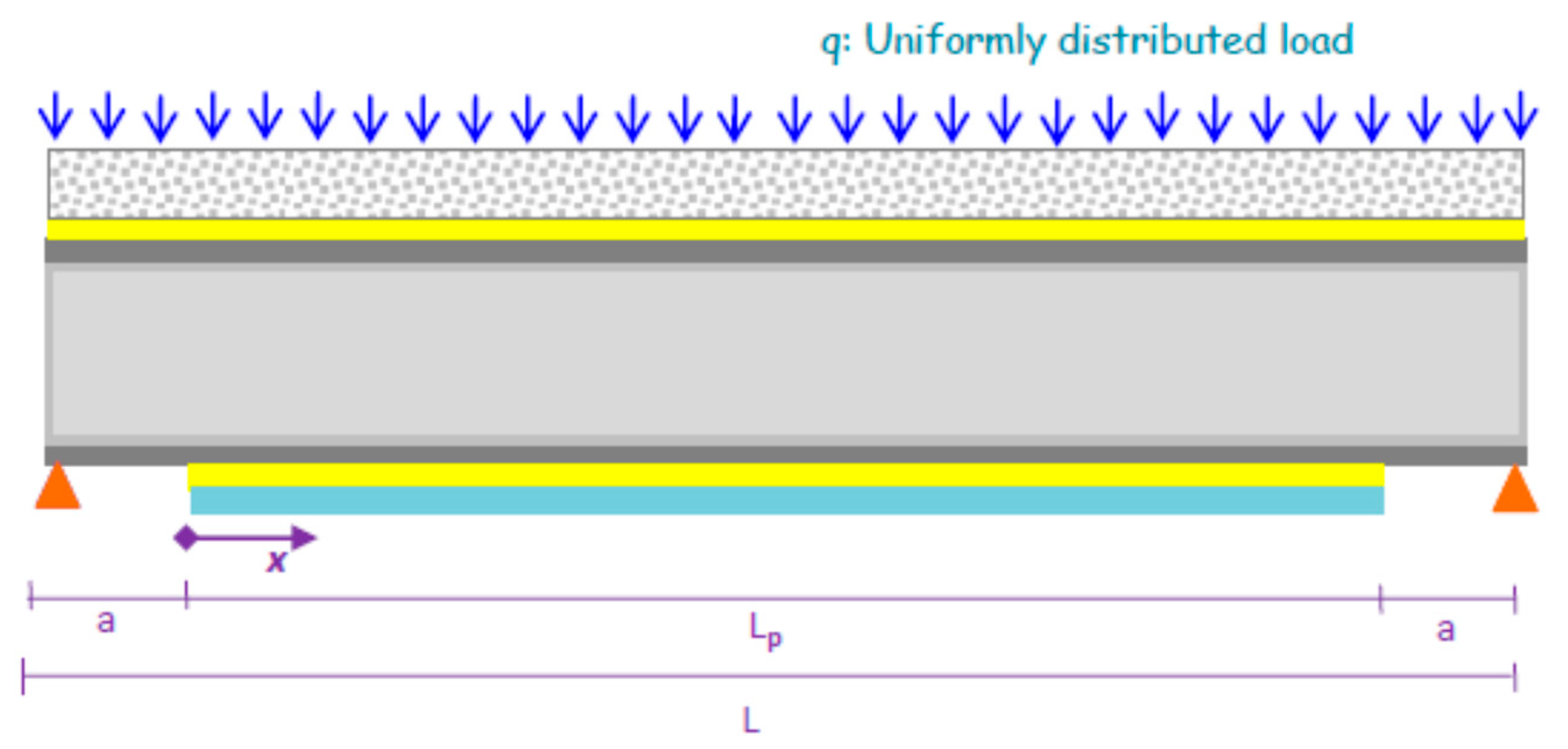
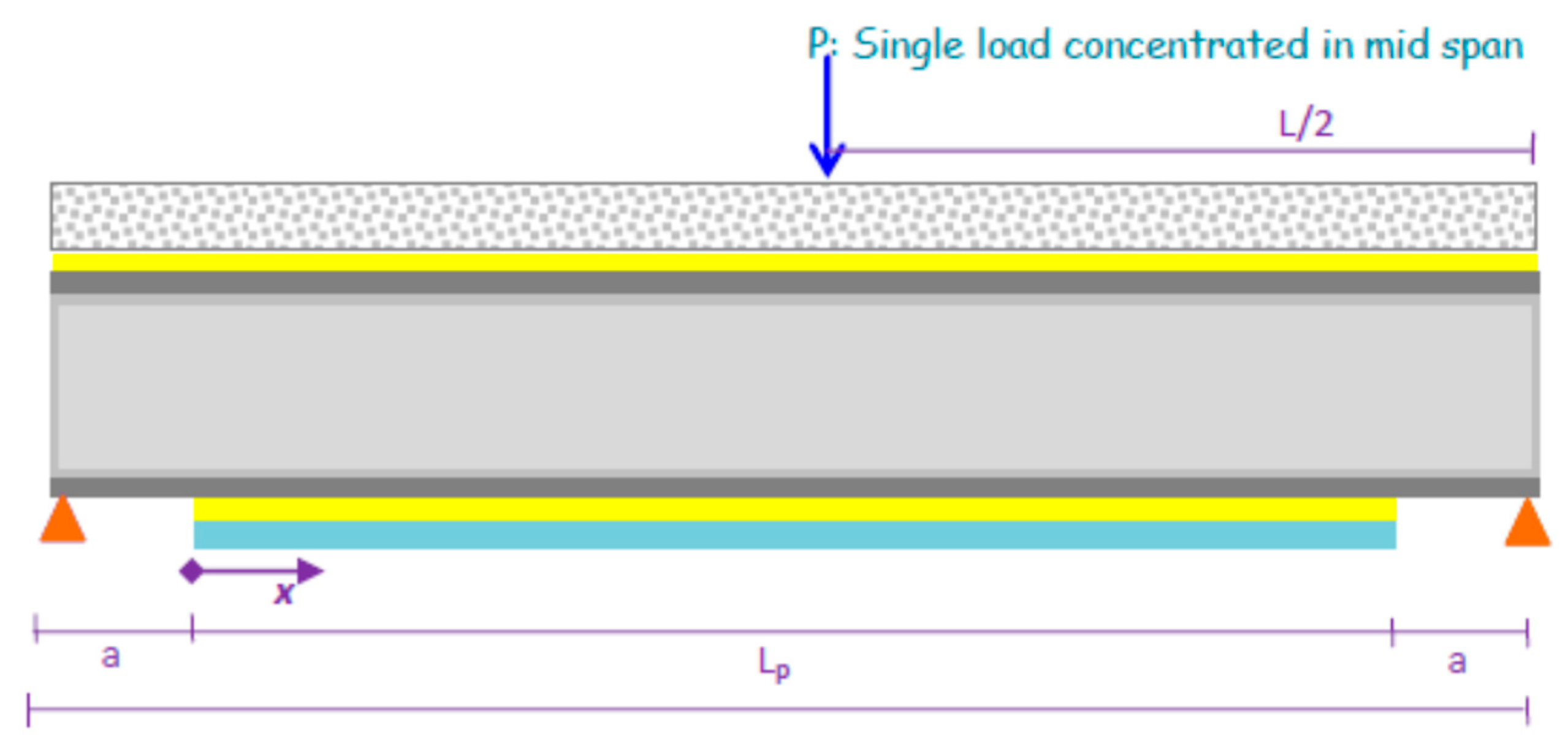
The formulation of the underlying assumptions and development of the static equilibrium model for the composite system.

-

The derivation of internal force expressions within an infinitesimal beam element $dx$, facilitating the analysis of load transfer mechanisms across the steel–concrete interface.

-

The mathematical modeling of axial strain distributions in both the steel section and concrete slab, accounting for differential deformation under applied loads.

-

The determination of shear stress distributions along the interface, derived from relative displacements between the bonded materials.

-

The quantification of interfacial stresses and slip as functions of the connection strategy—whether through mechanical shear connectors, structural adhesive bonding, or a hybrid of both.

-

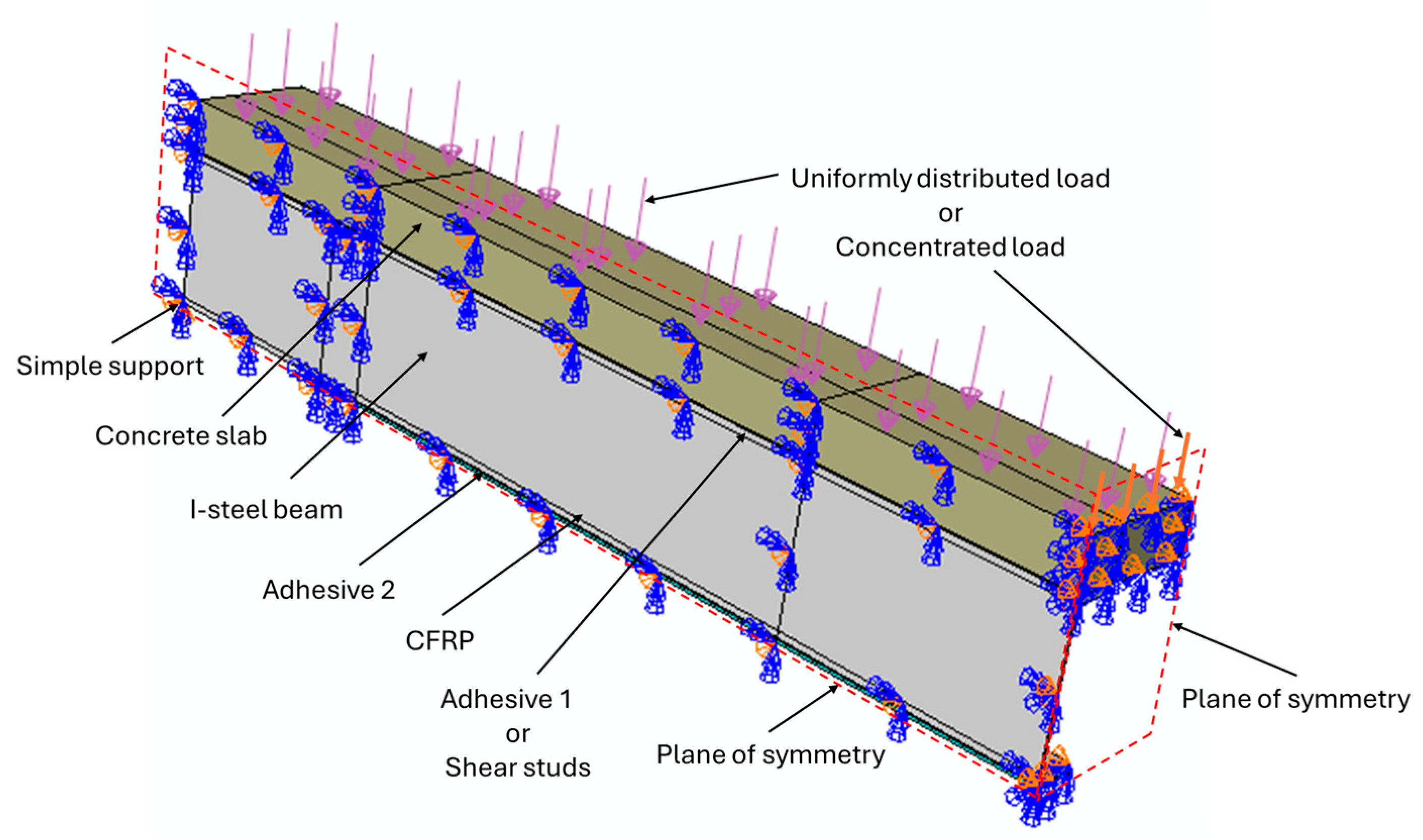
The development of a finite element simulation methodology to validate the analytical model and extend its applicability to various composite configurations and material systems.

2.1. Assumptions

This study aimed to compare the behavior of mechanically connected and adhesively bonded steel–concrete composite connections under flexural loading (Figure 1).

The analysis considers transverse shear stress and strain in the beam and plate, disregarding transverse normal stress. The authors extend their approach to steel–beam strengthening with a bonded composite plate [10,11,12,13], comparing it with finite element analysis based on the following assumptions:

-

The adhesive’s bending deformations are not considered.

-

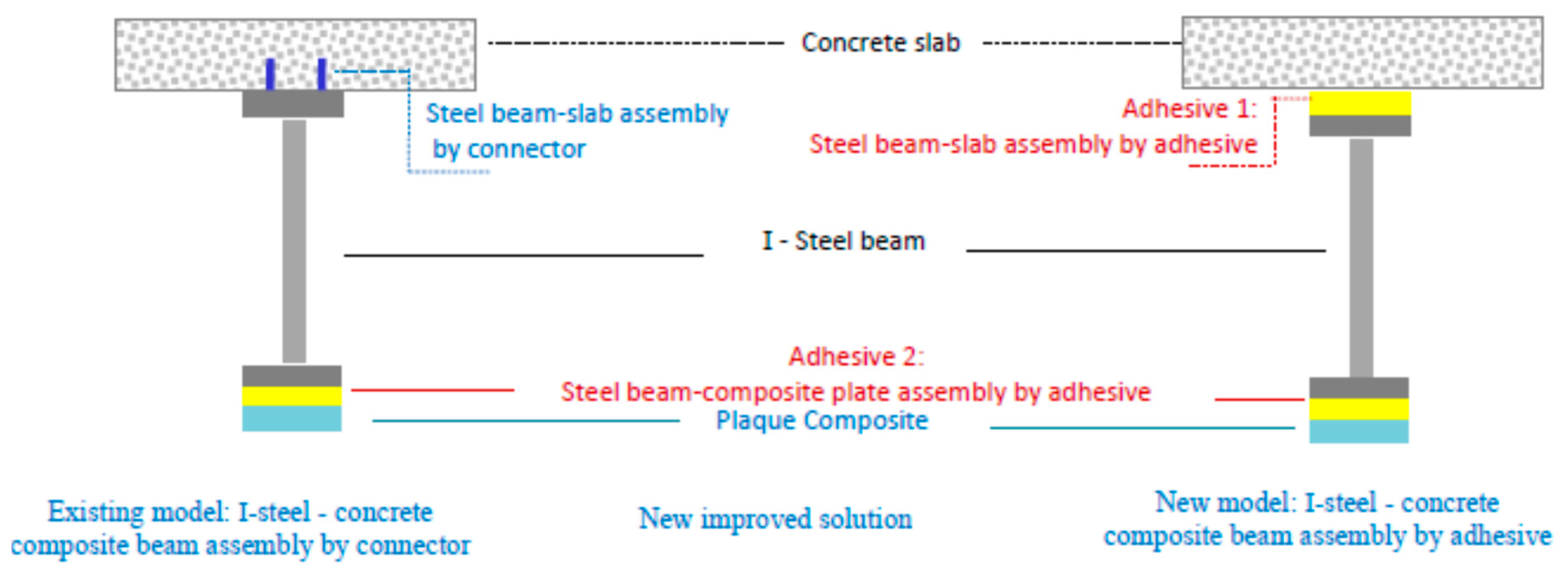
The composite–steel bond interface (Interface 2) is secure, but there is a slip between the concrete slab and the steel beam (Interface 1).

-

The materials considered are linear and elastic.

-

The beam is supported and shallow, ensuring that plane sections remain planar during bending.

-

The adhesive layer’s stress remains constant through the thickness.

-

The shear stress analysis supposes equal curvatures between the beam and plate, but the peel stress solution does not. Loading causes vertical separation between the steel beam and composite plate, resulting in interfacial normal stress in the adhesive layer.

-

The parabolic shear stress distribution is assumed through the depth of both the composite steel–concrete beam and the connected plate.

The analysis was conducted on simply supported composite I-steel–concrete beams reinforced by a composite plate under a uniformly distributed load (Figure 2) and under a concentrated load in the midspan (Figure 3).

The cross-section of the composite I-steel–concrete assembled by connectors and by adhesive is shown in Figure 4.

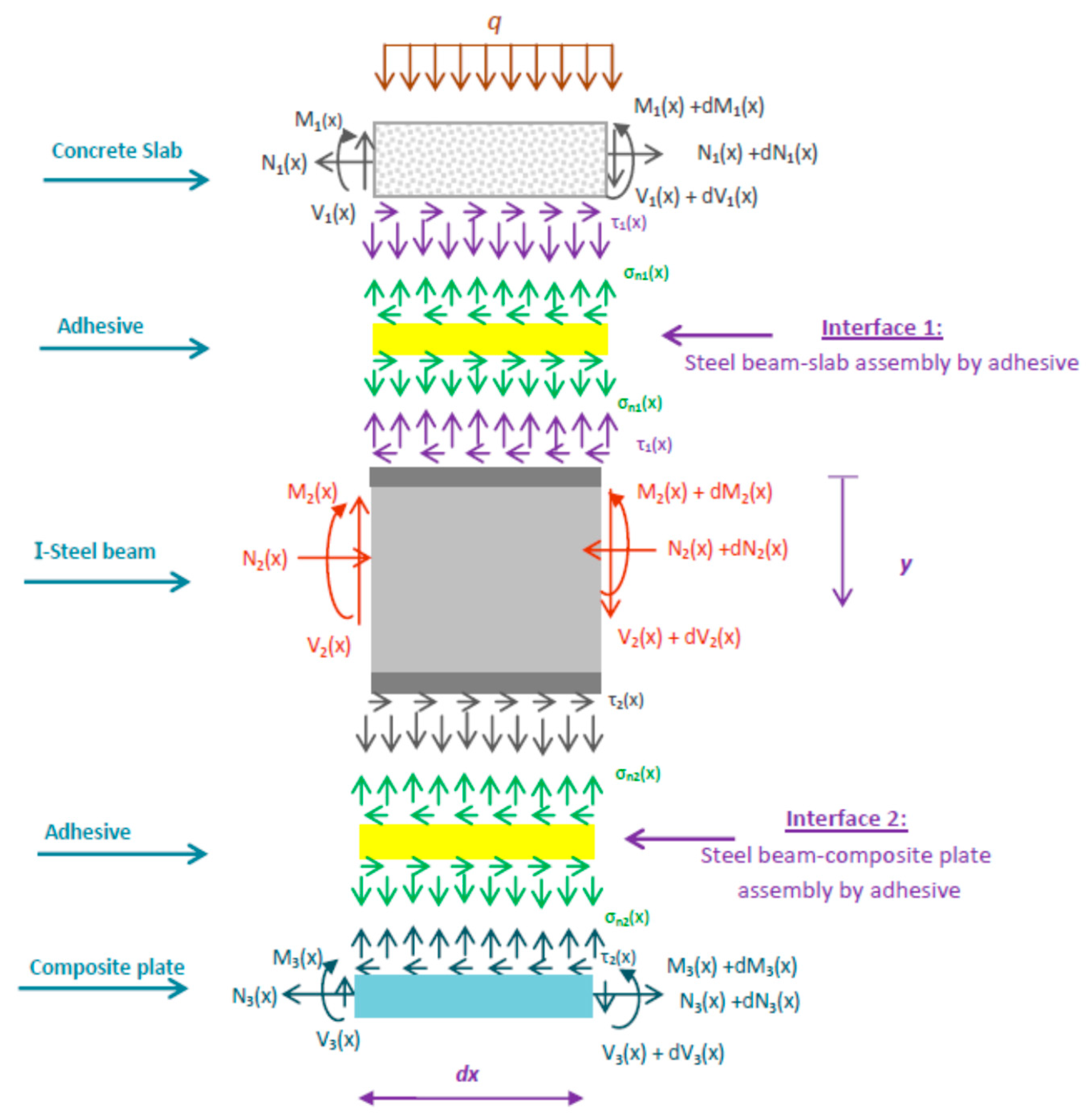
2.2. Internal Forces in the Interfaces

Internal forces in the infinitesimal element, $dx,$ of the I-steel–concrete beams are reinforced by a composite material plate consisting of four materials: a steel beam, concrete slab, adhesive layer, and composite reinforcement, which are given in Figure 5. All materials exhibit linear elastic behavior, with the adhesive layer transferring stresses from concrete to reinforcement. In the mathematical formulation, three indexes are defined as follows:

-

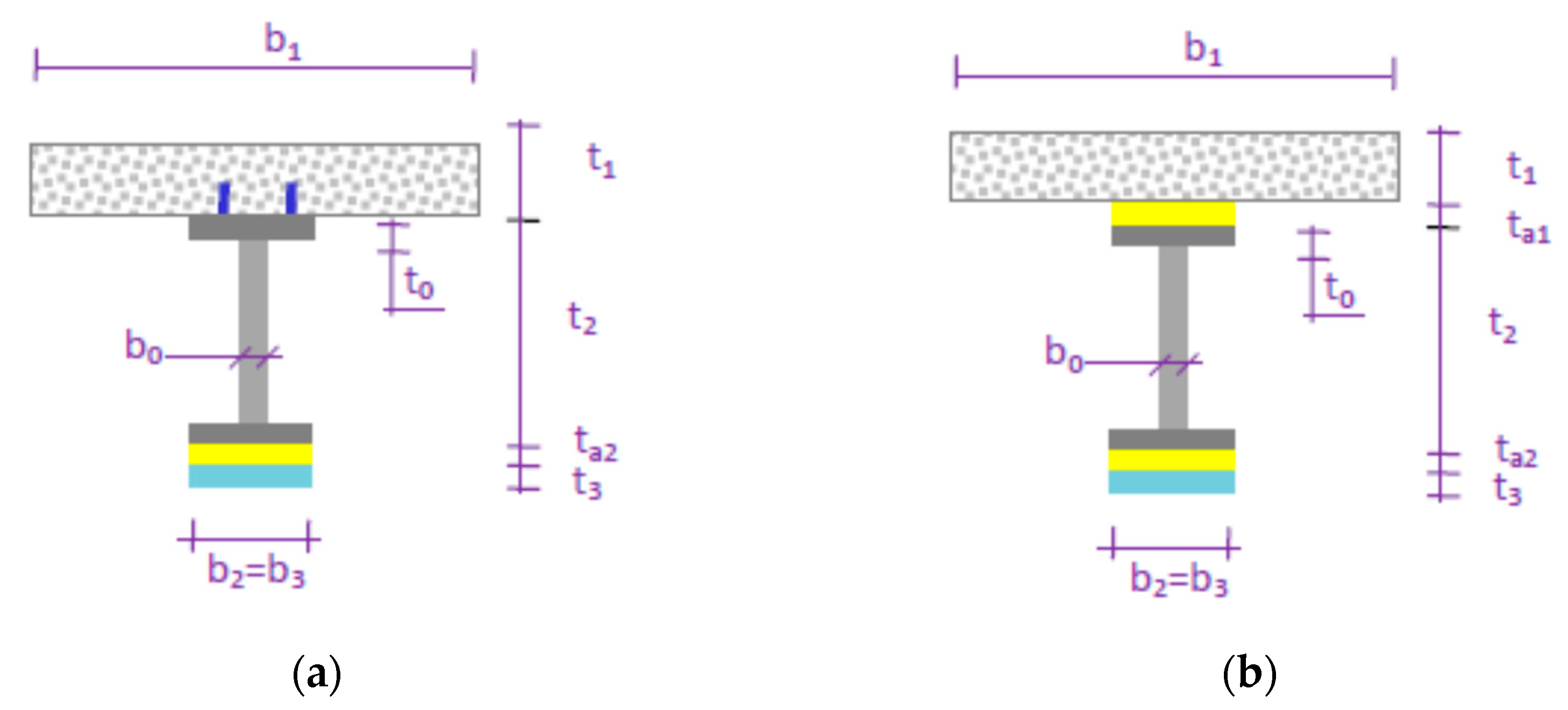
Index “1” corresponds to the first adherent “concrete slab”.

-

Index “2” corresponds to the second adherent “steel beam”.

-

Index “3” corresponds to the third adherent “composite reinforcement plate”.

2.3. Longitudinal Strains

The strains in the concrete near the adhesive 1 interface and the external steel beam and the strains in the steel beam near the adhesive 2 interface and the external composite plate can be expressed, respectively, as follows:

$${\epsilon }_i\left(x\right)={\displaystyle \frac{d{u}_i\left(x\right)}{dx}}={\epsilon }_i^{\left(M\right)}+{\epsilon }_i^{\left(N\right)} \left(i=1, 2, 3\right),$$

(1)

where $u_i\left(x\right)$ represents longitudinal displacements at the bottom of the concrete slab, the top of the steel beam, and the top of the composite, respectively.

${\epsilon }_i^{\left(M\right)}$ represents the strains induced by the bending moment at the concrete slab, the beam steel, and the plate of the composite, respectively, which are written as follows:

$${\epsilon }_i^{\left(M\right)}(x)={\displaystyle \frac{d{u}_i^{\left(M\right)}\left(x\right)}{dx}}={\displaystyle \frac{y_i}{E_i{I}_i}}{M}_i(x) \left(i=1, 2, 3\right),$$

(2)

where $E_i$ is the elastic moduli and $I_i$ represents the second moments of area. The subscripts 1, 2, and 3 indicate the elements of concrete, the steel beam, and composite plate, respectively. $M_i\left(x\right)$ represents the bending moments while $y_i$ represents the distances from the bottom of the concrete slab and the top of the steel beam to their respective centroids.

${\epsilon }_i^{\left(N\right)}$ represents the unknown longitudinal strains of the concrete, steel beam, and composite plate, respectively, at the adhesive interface due to the longitudinal forces. These strains are given as follows:

$${\epsilon }_i^{\left(N\right)}(x)={\displaystyle \frac{d{u}_i^{\left(N\right)}\left(x\right)}{dx}} \left(i=1, 2, 3\right),$$

(3)

where $u_1^{\left(N\right)}$ is the longitudinal force-induced displacement at the interface between the concrete slab and adhesive 1, and the interface between the steel beam and adhesive 1. $u_2^{\left(N\right)}$ is the longitudinal force-induced displacement at the interface between the steel beam and adhesive 2. $u_3^{\left(N\right)}$ is the longitudinal force-induced displacement at the interface between the composite plate and adhesive 2.

2.4. Shear Stresses

To determine the unknown longitudinal strains, ${\epsilon }_i^{\left(N\right)}$, the present analysis incorporates the shear deformation behavior of the adherent materials. It is assumed that the shear stress field remains continuous across the adhesive–adherent interfaces, which is a reasonable approximation given the typically thin nature of the adhesive layer and the absence of delamination under service conditions. By invoking Hooke’s law for linear elastic materials, the shear stresses within each of the three adherent layers are expressed as follows:

$${\sigma }_{xy\left(i\right)}=G_i{\gamma }_{xy\left(i\right)} \left(i=1, 2, 3\right),$$

(4)

with

$${\gamma }_{xy\left(i\right)}={\displaystyle \frac{d{U}_i^{\left(N\right)}}{dy}}+{\displaystyle \frac{d{W}_i^{\left(N\right)}}{dx}} \left(i=1, 2, 3\right),$$

(5)

Here, $G_i$ represents the transverse shear moduli of the concrete slab, steel beam, and composite plate, respectively.

By neglecting the variations in transverse displacements induced by the longitudinal forces $W_i^{\left(N\right)}$ with the longitudinal coordinate $x$, we can obtain the following:

$${\gamma }_{xy\left(i\right)}\approx {\displaystyle \frac{d{U}_i^{\left(N\right)}}{dy}} \left(i=1, 2, 3\right),$$

(6)

Shear stress is required to satisfy the following conditions:

$${\sigma }_{xy\left(1\right)}(x,t_1)={\sigma }_{xy\left(2\right)}(x,0)=\tau \left(x\right)={\tau }_{a1},$$

(7)

$${\sigma }_{xy\left(1\right)}\left(x,0\right)=0, {\sigma }_{xy\left(2\right)}\left(x,t_2\right)={\tau }_{a2},{\sigma }_{xy\left(3\right)}\left(x,t_3\right)=0,$$

(8)

$${\sigma }_{xy\left(3\right)}(x,0)=\tau \left(x\right)={\tau }_{a2},$$

(9)

$${\sigma }_{xy\left(3\right)}(x,t_3)=0,$$

(10)

where $t_1$, $t_2$, and $t_3$ are the thicknesses of the concrete slab, the steel beam, and the composite plate, respectively.

Condition (7) follows from continuity and the assumption of constant shear stresses ($\tau \left(x\right)={\tau }_{a1}$) through the thickness of adhesive 1. Condition (8) states that there are no shear stresses at the surface of the concrete slab (i.e., at $y=0$) and at the surface of the steel beam (i.e., at $y=t_2$). Condition (9) also follows from continuity and the assumption of constant shear stresses ($\tau \left(x\right)={\tau }_{a2}$) through the thickness of adhesive 2. Condition (10) states that there is no shear stress at the surface of the composite surface.

These conditions yield the following:

$${\sigma }_{xy\left(1\right)}={\displaystyle \frac{\tau \left(x\right)}{t_1}}y,$$

(11)

$${\sigma }_{xy\left(2\right)}=\left(1+{\displaystyle \frac{\left(\frac{{\tau }_{a2}}{{\tau }_{a1}}-1\right)y}{t_2}}\right)\tau (x),$$

(12)

$${\sigma }_{xy\left(3\right)}=\left(1-{\displaystyle \frac{y}{t_3}}\right)\tau \left(x\right),$$

(13)

Assuming linear elastic material behavior, the shear strains in the concrete slab, steel beam, and externally bonded composite plate can be expressed as follows:

$${\gamma }_{xy\left(1\right)}={\gamma }_1=\left({\displaystyle \frac{{\tau }_{a1}}{G_1{t}_1}}\right)y,$$

(14)

$${\gamma }_{xy\left(2\right)}={\gamma }_2=\left(1+{\displaystyle \frac{\left(\frac{{\tau }_{a2}}{{\tau }_{a1}}-1\right)y}{t_2}}\right){\displaystyle \frac{{\tau }_{a1}}{G_2}},$$

(15)

$${\gamma }_{xy\left(3\right)}={\gamma }_3=\left(1-{\displaystyle \frac{y}{t_3}}\right){\displaystyle \frac{{\tau }_{a2}}{G_3}},$$

(16)

The longitudinal displacement functions $U_1^{\left(N\right)}$ for the concrete slab, $U_2^{\left(N\right)}$ for the steel beam, and $U_3^{\left(N\right)}$ for the composite plate, due to the longitudinal forces, are expressed as follows:

$$U_i^{\left(N\right)}(y)=u_i^{\left(N\right)}(0)+{\int }_0^{t_i}{\gamma }_i(y)dy \left(i=1, 2, 3\right),$$

(17)

where $u_1^{\left(N\right)}(0)$ is the displacement due to the longitudinal forces at the top surface of the upper adherent and $u_2^{\left(N\right)}(0)$ is the displacement due to the longitudinal force at the interface between adhesive 1 and lower adherent.

Under the assumption of perfect bonding at the interfaces, displacement continuity is preserved across the adhesive–adherent boundaries. Specifically, at Interface 1—between adhesive 1 and its adjacent adherents—the axial displacement field remains continuous. Consequently, the displacement $u_2^{\left(N\right)}$ within adhesive 1 must be equal to the displacement of the lower adherent at Interface 1, while the displacement at the interface between adhesive 1 and the upper adherent must match the corresponding displacement of the upper adherent at the same location.

Similarly, at Interface 2—between adhesive 2 and its associated adherents—the perfect bond condition ensures the continuity of displacements. Therefore, the displacement $u_3^{\left(N\right)}$ within adhesive 2 must coincide with that of the lower adherent at Interface 2, and the displacement at the interface with the upper adherent must be equal to the displacement of the upper adherent at that point.

The longitudinal resultant forces for the concrete slab, the steel beam, and the composite plate are, respectively, given as follows:

$$N_i^N=b_i{\int }_0^{t_i}{\sigma }_i^N(y)dy \left(i=1, \mathrm{2,3}\right),$$

(18)

where ${\sigma }_i^N$ represents longitudinal normal stresses for the concrete slab, the steel beam, and the composite plate, respectively. $b_i$ represents the corresponding widths.

By expressing these stresses as functions of the corresponding displacement fields and substituting Equation (17) into the displacement expressions, Equation (18) can be reformulated as follows:

$$N_1=E_1{b}_1{\int }_0^{t_1}{\displaystyle \frac{d{U}_1^{\left(N\right)}}{dx}}dy=E_1{A}_1\left({\displaystyle \frac{d{U}_1^{\left(N\right)}}{dx}}-{\displaystyle \frac{{\rho }_1{t}_1}{G_1}}{\displaystyle \frac{d\tau \left(x\right)}{dx}}\right),$$

(19)

$$N_2=E_2{b}_2{\int }_0^{t_2}{\displaystyle \frac{d{U}_2^{\left(N\right)}}{dx}}dy=E_2{A}_2\left({\displaystyle \frac{d{U}_2^{\left(N\right)}}{dx}}-\left({\displaystyle \frac{{\tau }_{a2}}{{\tau }_{a1}}}-1\right){\displaystyle \frac{{\rho }_2{t}_2}{G_2}}{\displaystyle \frac{d\tau \left(x\right)}{dx}}\right),$$

(20)

$$N_3=E_3{b}_3{\int }_0^{t_3}{\displaystyle \frac{d{U}_3^{\left(N\right)}}{dx}}dy=E_3{A}_3\left({\displaystyle \frac{d{U}_3^{\left(N\right)}}{dx}}-{\displaystyle \frac{{\rho }_3{t}_3}{G_3}}{\displaystyle \frac{d\tau \left(x\right)}{dx}}\right),$$

(21)

with

$${\rho }_i={\displaystyle \frac{I_i}{Q_i\frac{t_i}{2}}} \left(i=1, 2, 3\right),$$

(22)

where ${\rho }_i$ represents the efficiencies of the different adherents and $Q_i$ represents the first moments of area (static moments) of the different adherents.

Hence, the longitudinal strains induced by the longitudinal forces given in Equation (3) can be expressed as follows:

$${\epsilon }_1^{\left(N\right)}\left(x\right)={\displaystyle \frac{d{u}_1^{\left(N\right)}\left(x\right)}{dx}}={\displaystyle \frac{N_1}{E_1{A}_1}}+{\displaystyle \frac{{\rho }_1{t}_1}{G_1}}{\displaystyle \frac{d\tau \left(x\right)}{dx}},$$

(23)

$${\epsilon }_2^{\left(N\right)}\left(x\right)={\displaystyle \frac{d{u}_2^{\left(N\right)}\left(x\right)}{dx}}={\displaystyle \frac{N_2}{E_2{A}_2}}+\left({\displaystyle \frac{{\tau }_{a2}}{{\tau }_{a1}}}-1\right){\displaystyle \frac{{\rho }_2{t}_2}{G_2}}{\displaystyle \frac{d\tau \left(x\right)}{dx}},$$

(24)

$${\epsilon }_3^{\left(N\right)}\left(x\right)={\displaystyle \frac{d{u}_3^{\left(N\right)}\left(x\right)}{dx}}={\displaystyle \frac{N_3}{E_3{A}_3}}+{\displaystyle \frac{{\rho }_3{t}_3}{G_3}}{\displaystyle \frac{d\tau \left(x\right)}{dx}},$$

(25)

Substituting Equations (23), (24), (25), and (4) into Equations (1) and (2), respectively, the latter equations become the following:

$${\epsilon }_1={\displaystyle \frac{d{u}_1^{\left(M\right)}\left(x\right)}{dx}}+{\displaystyle \frac{d{u}_1^{\left(N\right)}\left(x\right)}{dx}}={\displaystyle \frac{y_1}{E_1{I}_1}}{M}_1\left(x\right)+{\displaystyle \frac{N_1\left(x\right)}{E_1{A}_1}}+{\displaystyle \frac{{\rho }_1{t}_1}{G_1}}{\displaystyle \frac{d\tau \left(x\right)}{dx}},$$

(26)

$${\epsilon }_2={\displaystyle \frac{d{u}_2^{\left(M\right)}\left(x\right)}{dx}}+{\displaystyle \frac{d{u}_2^{\left(N\right)}\left(x\right)}{dx}}={\displaystyle \frac{y_2}{E_2{I}_2}}{M}_2\left(x\right)-{\displaystyle \frac{N_2\left(x\right)}{E_2{A}_2}}-\left({\displaystyle \frac{{\tau }_{a2}}{{\tau }_{a1}}}-1\right){\displaystyle \frac{{\rho }_2{t}_2}{G_2}}{\displaystyle \frac{d\tau \left(x\right)}{dx}},$$

(27)

$${\epsilon }_3={\displaystyle \frac{d{u}_3^{\left(M\right)}\left(x\right)}{dx}}+{\displaystyle \frac{d{u}_3^{\left(N\right)}\left(x\right)}{dx}}={\displaystyle \frac{y_3}{E_3{I}_3}}{M}_3\left(x\right)-{\displaystyle \frac{N_3\left(x\right)}{E_3{A}_3}}-{\displaystyle \frac{{\rho }_3{t}_3}{G_3}}{\displaystyle \frac{d\tau \left(x\right)}{dx}},$$

(28)

The shear stress in adhesives 1 and 2 or the connector (studs) and adhesive 2 can be expressed as follows:

$$\tau \left(x\right)=K_{s1}\left[u_1\left(x\right)-u_2\left(x\right)\right],$$

(29)

$$\tau \left(x\right)=K_{s2}\left[u_2\left(x\right)-u_3\left(x\right)\right],$$

(30)

To make this study simple, we propose that elements 2 and 3 are in full connection, i.e., we replace both elements 2 and 3 with an equivalent element noted 2r, so Equations (29) and (30) become a single equation:

$$\tau \left(x\right)=K_s\left[u_1\left(x\right)-u_{2r}\left(x\right)\right],$$

(31)

with

$$K_s=\left\{\begin{array}{l}{\displaystyle \frac{G_{a1}}{t_{a1}}} \mathrm{if} e_a<120 \mathrm{mm}, \mathrm{shear} \mathrm{stifness} \mathrm{of} \mathrm{adhesive} 1\\ {\displaystyle \frac{G_{a2}}{t_{a2}}} \mathrm{if} e_a<120 \mathrm{mm}, \mathrm{shear} \mathrm{stifness} \mathrm{of} \mathrm{adhesive} 2\\ {\displaystyle \frac{N_a{b}_a{L}_a{G}_{a1}}{b_{0}L{t}_{a1}}} \mathrm{if} e_a>120 \mathrm{mm}, \mathrm{shear} \mathrm{stifness} \mathrm{of} \mathrm{adhesive} \mathrm{by} \mathrm{band} \\ {\displaystyle \frac{N_{co}{K}_c}{e}} \mathrm{is} \mathrm{shear} \mathrm{stiffness} \mathrm{of} \mathrm{the} \mathrm{connector}\end{array}\right.,$$

(32)

where $G_a$ and $t_a$ are the shear modulus and thickness of the adhesive, respectively. $K_c$, $N_{co}$ and $e$ are the connector’s rigidity modulus, the range’s number of connectors and the spacing between the connectors along $x$, respectively. And $b_a$ and $L_a$ are the adhesive width and overlap length and $e_a$ is the clear spacing between the strips along $x$.

According to Oehlers et al. [14] and Silva et al. [15], a bolt connector has a linear behavior until 50% of its maximum force resistance is reached. The same authors relate the connector’s rigidity modulus ($E_c$) with the maximum force ($F_{max}$), the diameter of its base ($d$), and the compression resistance of the concrete ($f_{ck}$), as shown in Equations (19) and (20):

$$K_c={\displaystyle \frac{F_{max}}{d\left(0.16-0.00172f_{ck}\right)}},$$

(33)

$$F_{max}=0.5A_{sh}\sqrt{f_{ck}{E}_c},$$

(34)

where $A_{sh}$ is the area of the cross-section of the connector’s base. The dimensions in these equations are given in N, mm, and MPa.

According to the NBR-8800 standard [16], the connector can withstand a maximum force ($F_{max}$) given by the following equation:

$$F_{max}=\min \left\{\begin{array}{c}{\displaystyle \frac{0.5A_{sh}\sqrt{f_{ck}{E}_c}}{{\gamma }_{sh}}}\\ {\displaystyle \frac{A_{sh}{f}_u}{{\gamma }_{sh}}}\end{array}\right.,$$

(35)

where $f_u$ is the ultimate stress resistance of the connector and ${\gamma }_{sh}=1.25$.

According to the NBR-8800 standard [16], the spacing between the connectors is limited to six times the diameter of the connector.

In this study, five different connection modes were analyzed, from the assembly of full connectors to full adhesive assembly. Figure 6 presents a composite steel beam–concrete slab system incorporating hybrid connectors and adhesive bonding. To mitigate the shear lag effect [7,10], the adhesive bonding was initiated at the beam ends, where stress concentrations are typically highest. This strategic placement of bonding is essential for enhancing the structural stability of the composite system.

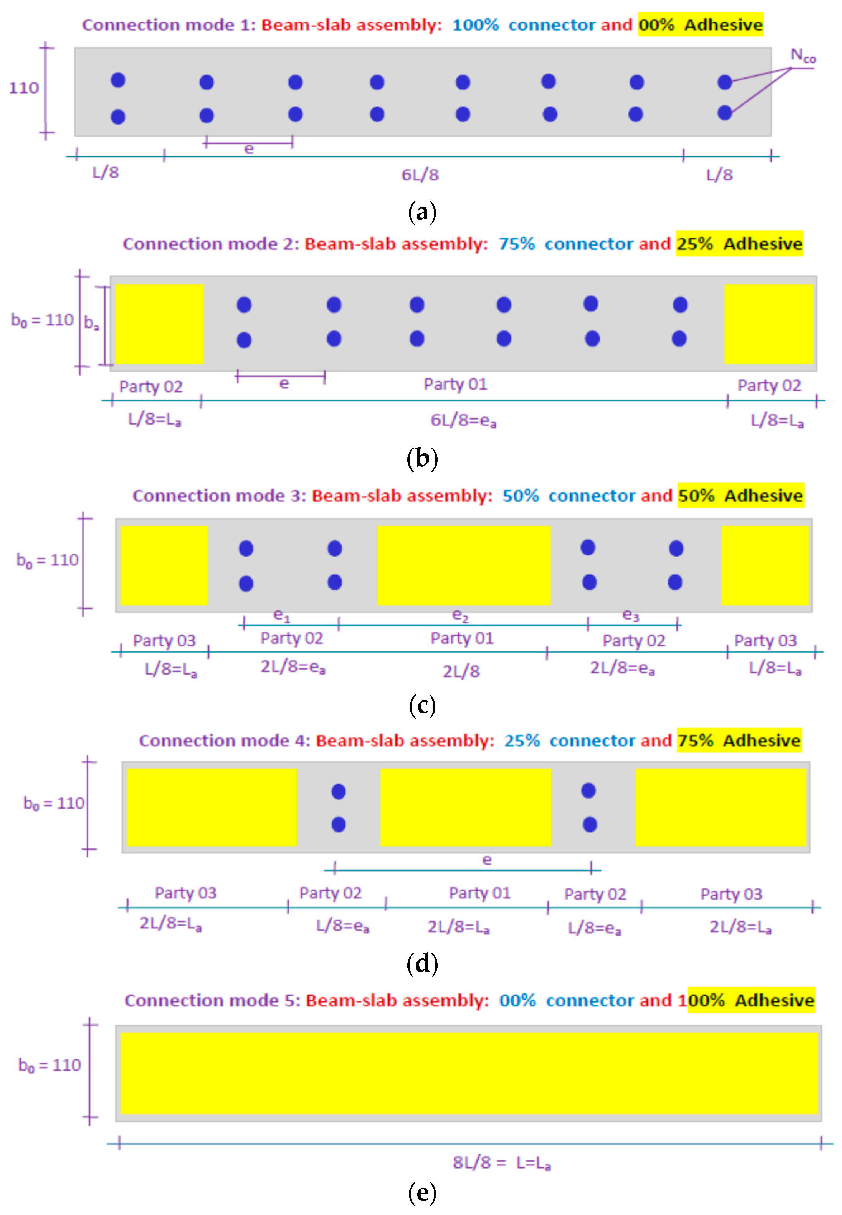
2.4.1. Case 1: Interface Shear Stress Distribution with Only Connectors or Adhesive

This case corresponds to Figure 6a,e. By only differentiating the expression of the shear stress (Equation (17)) in the adhesive and connectors (studs), we obtained the following:

$${\displaystyle \frac{d\tau \left(x\right)}{dx}}=K_s\left[{\displaystyle \frac{{du}_1\left(x\right)}{dx}}-{\displaystyle \frac{d{u}_{2r}\left(x\right)}{dx}}\right],$$

(36)

By considering the horizontal equilibrium, we obtained the following:

$${\displaystyle \frac{d{N}_1(x)}{dx}}=\tau (x),$$

(37)

$${\displaystyle \frac{d{N}_{2r}\left(x\right)}{dx}}=-\tau (x),$$

(38)

where

$$N_1(x)=N(x)={\int }_0^x\tau \left(x\right),$$

(39)

$$N_{2r}\left(x\right)=-N\left(x\right)=-{\int }_0^x\tau \left(x\right),$$

(40)

The condition of equal curvatures ($\phi$) in the steel beam and the slab provides the following relationship:

$$\phi ={\displaystyle \frac{M_1\left(x\right)}{E_1{A}_1}}={\displaystyle \frac{M_{2r}\left(x\right)}{E_{2r}{A}_{2r}}}={\displaystyle \frac{M_1\left(x\right)+M_{2r}\left(x\right)}{E_1{A}_1+E_{2r}{A}_{2r}}},$$

(41)

Under the application of a vertical load, the variation in the bending moment along an infinitesimal beam segment $dx$ is balanced not only by the internal shear force—as described by the classical beam theory—but also by the additional contribution from the interface connection system:

$$d{M}_1\left(x\right)=V_{1}dx-\tau \left(x\right)y_1,$$

(42)

$$d{M}_{2r}\left(x\right)=V_{2r}dx-\tau \left(x\right)y_{2r},$$

(43)

The moment of equilibrium of the differential segment of the beam in Figure 2 gives the following:

$$M\left(x\right)=M_1\left(x\right)+M_{2r}\left(x\right)+N\left(y_1+y_{2r}+t_{a1}\right),$$

(44)

By substituting Equations (26), (27) and (28) into Equation (36), we can obtain the following:

$$\begin{gathered} {\displaystyle \frac{d\tau \left(x\right)}{dx}}=K_s\left[{\displaystyle \frac{y_1}{E_1{I}_1}}{M}_1(x)-{\displaystyle \frac{N_1\left(x\right)}{E_1{A}_1}}-{\displaystyle \frac{{\rho }_1{t}_1}{G_1}}{\displaystyle \frac{d\tau \left(x\right)}{dx}}+{\displaystyle \frac{y_{2r}}{E_{2r}{I}_{2r}}}{M}_{2r}(x) \\ +{\displaystyle \frac{N_{2r}\left(x\right)}{E_{2r}{A}_{2r}}}\right.\left.-{\displaystyle \frac{{\rho }_{2r}{t}_{2r}}{G_{2r}}}{\displaystyle \frac{d\tau \left(x\right)}{dx}}\right], \end{gathered}$$

(45)

Deriving Equation (45) yields the following:

$$\begin{gathered} {\displaystyle \frac{1}{K_s}}{\displaystyle \frac{d^2\tau \left(x\right)}{d{x}^2}}=\left[{\displaystyle \frac{y_1}{E_1{I}_1}}{\displaystyle \frac{d{M}_1\left(x\right)}{dx}}-{\displaystyle \frac{1}{E_1{A}_1}}{\displaystyle \frac{d{N}_1(x)}{dx}}-{\displaystyle \frac{{\rho }_1{t}_1}{G_1}}{\displaystyle \frac{d^2\tau \left(x\right)}{d{x}^2}}+{\displaystyle \frac{y_{2r}}{E_{2r}{I}_{2r}}}{\displaystyle \frac{{dM}_{2r}\left(x\right)}{dx}} \\ +{\displaystyle \frac{1}{E_{2r}{A}_{2r}}}\right.\left.{\displaystyle \frac{d{N}_{2r}\left(x\right)}{dx}}-{\displaystyle \frac{{\rho }_{2r}{t}_{2r}}{G_{2r}}}{\displaystyle \frac{d^2\tau (x)}{d{x}^2}}\right], \end{gathered}$$

(46)

The substitution of the shear forces (Equations (39) and (40)) and axial forces (Equations (19), (20), (21), (26), (27) and (28)) into Equation (46) gives the following governing differential equation for the interfacial shear stress:

$$\begin{gathered} {\displaystyle \frac{1}{K_s}}{\displaystyle \frac{d^2\tau \left(x\right)}{d{x}^2}}-K_1\left[{\displaystyle \frac{\left(y_1+y_{2r}\right)\left(y_1+y_{2r}+t_{1a}\right)}{{E_1{I}_1+E}_{2r}{I}_{2r}}}+{\displaystyle \frac{1}{E_1{A}_1}}+{\displaystyle \frac{1}{E_{2r}{A}_{2r}}}\right]{\displaystyle \frac{d\tau \left(x\right)}{dx}} \\ +K_1{\displaystyle \frac{\left(y_1+y_{2r}\right)}{{E_1{I}_1+E}_{2r}{I}_{2r}}}V\left(x\right)=0, \end{gathered}$$

(47)

where

$$K_1=\left\{\begin{array}{cc}\frac{1}{\frac{t_{a1}}{G_{a1}}+\frac{{\rho }_1{t}_1}{G_1}+\frac{{\rho }_{2r}{t}_{2r}}{G_{2r}}} \mathrm{for} \mathrm{adhesive} \hfill & \hspace{1em}\hspace{1em}\hspace{1em}\hspace{1em}\hspace{1em}\hspace{1em}\hspace{1em}\hspace{1em}\hspace{1em}\hspace{1em}\hspace{1em}\hspace{1em}\mathrm{(48)}\\ {\displaystyle \frac{1}{\frac{{\rho }_1{t}_1}{G_1}+\frac{{\rho }_{2r}{t}_{2r}}{G_{2r}}}} \mathrm{for} \mathrm{connector,}\hfill & \hspace{1em}\hspace{1em}\hspace{1em}\hspace{1em}\hspace{1em}\hspace{1em}\hspace{1em}\hspace{1em}\hspace{1em}\hspace{1em}\hspace{1em}\hspace{1em}\mathrm{(49)}\end{array}\right.$$

For analytical tractability, the general solutions to Equation (47) are derived under loading conditions that consist of either a concentrated point load or uniformly distributed load, which are applied over a portion, over the entire span of the beam, or a combination of both.

For such loadings, ${\displaystyle \frac{d^{2}V\left(x\right)}{d{x}^2}}=0$ and the general solution of Equation (47) is given as follows:

$$\tau \left(x\right)=B_1{e}^{\lambda x}+B_2{e}^{-\lambda x}+\beta V\left(x\right),$$

(50)

where

$${\lambda }^2=K_1{b}_2\left[{\displaystyle \frac{\left(y_1+y_{2r}\right)\left(y_1+y_{2r}+t_{a1}\right)}{E_1{I}_1+E_{2r}{I}_{2r}}}+{\displaystyle \frac{1}{E_1{A}_1}}+{\displaystyle \frac{1}{E_{2r}{A}_{2r}}}\right],$$

(51)

$$\beta ={\displaystyle \frac{K_1}{{\lambda }^2}}\left[{\displaystyle \frac{1}{E_1{A}_1}}+{\displaystyle \frac{1}{E_{2r}{A}_{2r}}}\right],$$

(52)

$B_1$ and $B_2$ are constant coefficients, the values of which are determined by enforcing the appropriate boundary conditions.

The relative slip strain at the interface is calculated as follows:

$${\displaystyle \frac{dS\left(x\right)}{dx}}={\displaystyle \frac{d{u}_1\left(x\right)}{dx}}-{\displaystyle \frac{d{u}_{2r}\left(x\right)}{dx}}={\epsilon }_1(x)-{\epsilon }_{2r}(x),$$

(53)

As indicated in the assumptions section, the slide of adhesive is proportional to the shear force $\tau \left(x\right)$, and the constant of proportionality is the adhesive stiffness $K_{a1}$:

$${\tau }_{a1}=\tau \left(x\right)=K_{a1}\left[u_1\left(x\right)-u_{2r}\left(x\right)\right]\iff \tau \left(x\right)=K_{a1}\cdot S\left(x\right),$$

(54)

where $S\left(x\right)$ represents the slip between adherents.

This study focuses on the structural behavior of simply supported composite beams subjected to midspan concentrated loads and/or uniformly distributed loads along the span (Figure 7) so that $\tau \left(x\right)=0$ and $d\tau \left(x\right)/dx=0$ at $x=L/2$.

With these conditions, the shear stress solution for $0\le x\le L/2$ is given by the following:

$$\tau (x)={\displaystyle \frac{\beta P}{2}}\left[{\displaystyle \frac{e^{-\lambda \left(\frac{L}{2}-x\right)}-e^{\lambda \left(\frac{L}{2}-x\right)}}{(e^{-\lambda \frac{L}{2}}+e^{\lambda \frac{L}{2}})}}+1\right],$$

(55)

where $P=F$ for the concentrated load or $P=qL$ for the uniformly distributed load.

The interfacial slip due to the load is then given by the following:

$$S(x)={\displaystyle \frac{\beta P}{2K_s}}\left[{\displaystyle \frac{e^{-\lambda \left(\frac{L}{2}-x\right)}-{\frac{\beta P}{2}e}^{\lambda \left(\frac{L}{2}-x\right)}}{(e^{-\lambda \frac{L}{2}}+e^{\lambda \frac{L}{2}})}}+1\right],$$

(56)

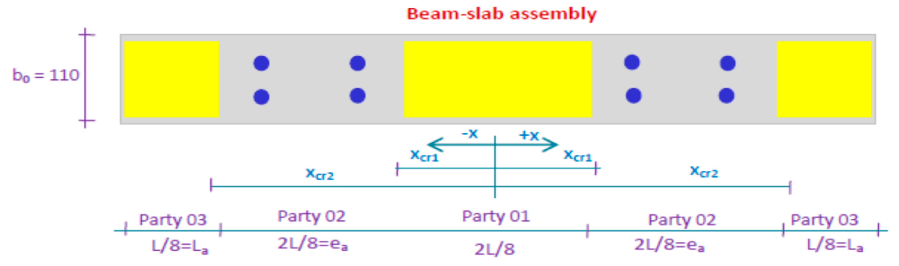
2.4.2. Case 2: Interface Shear Stress Distribution with Both Connectors and Adhesives

This case corresponds to Figure 6b–d. The beam–slab with a variable connection mode refers to a beam–slab with variable geometric characteristics of the section along the $x$ abscissa. To simplify the problem and remain in representative cases, we considered the beam–slab with different parties, as shown in Figure 8.

The beam has three parts connected by two types of connection. We consider that the transition between these three parts occurs by jumping at an abscissa $(x_{cri}, i=1,n)$, with $n$ representing the number of intersections between these parts. The coefficients $B_1$, $B_2$, and $\beta ,$ which are used in Equation (34), will have different values in adhesive and connector zones. Equation (34) is then redefined in each of these zones to consider this difference:

$${\tau }^{\left(i\right)}\left(x\right)=K_s^{\left(i\right)}\left[u_c^{\left(i\right)}\left(x\right)-u_s^{\left(i\right)}\left(x\right)\right] \left(i=1, 2, 3\right),$$

(57)

and the following is also obtained:

$${\tau }^{\left(1\right)}\left(x\right)=B_1^{\left(1\right)}{e}^{{\lambda }_{1}x}+B_2^{\left(1\right)}{e}^{{\lambda }_{1}x}+{\beta }^{\left(1\right)}V\left(x\right) \left(i=1, 2, 3\right),$$

(58)

where subscript (1) refers to part 1, subscript (2) refers to part 2, and subscript (3) refers to part 3 of the beam (Figure 8).

The three equations include six integration constants that can be determined by applying the boundary conditions. Two of the boundary conditions are identical to those used in the simply supported beam with only an adhesive or connector (Case 1); the other four conditions are defined to represent the compatibility of shear stress between parts 1, 2, and 3 at the abscissa $(x_{cri}, i=1,n)$:

$$\left\{\begin{array}{c}{\tau }^{\left(1\right)}\left(x_{cr1}\right)={\tau }^{\left(2\right)}\left(x_{cr1}\right)\\ {\tau }^{\left(2\right)}\left(x_{cr2}\right)={\tau }^{\left(3\right)}\left(x_{cr2}\right)\end{array}\right.,$$

(59)

$$\left\{\begin{array}{c}{\left.{\displaystyle \frac{{d\tau }^{\left(1\right)}}{dx}}\right|}_{x_{cr1}}={\left.{\displaystyle \frac{{d\tau }^{\left(2\right)}}{dx}}\right|}_{x_{cr1}}\\ {\left.{\displaystyle \frac{{d\tau }^{\left(2\right)}}{dx}}\right|}_{x_{cr2}}={\left.{\displaystyle \frac{{d\tau }^{\left(3\right)}}{dx}}\right|}_{x_{cr2}}\end{array}\right.,$$

(60)

The expression of the global shear stress for hybrid connection with the adhesive and connectors is given by the following:

$$\tau (x)=\left\{\begin{array}{l}{\tau }^{\left(1\right)}\left(x\right) \mathrm{if} 0\le x\le x_{cr1}\\ {\tau }^{\left(2\right)}\left(x\right) \mathrm{if} x_{cr1}\le x\le x_{cr2}\\ {\tau }^{\left(3\right)}(x) \mathrm{if} x_{cr2}\le x\le {\displaystyle \frac{L}{2}}\end{array}\right.,$$

(61)

And, finally, the interfacial slip is given by the following:

$$S(x)=\left\{\begin{array}{l}{\displaystyle \frac{{\tau }^{\left(1\right)}\left(x\right)}{K_s^{\left(1\right)}}} \mathrm{if} 0\le x\le x_{cr1}\\ {\displaystyle \frac{{\tau }^{\left(2\right)}\left(x\right)}{K_s^{\left(1\right)}+K_s^{\left(2\right)}}} \mathrm{if} x_{cr1}\le x\le x_{cr2}\\ {\displaystyle \frac{{\tau }^{\left(3\right)}\left(x\right)}{K_s^{\left(1\right)}+K_s^{\left(2\right)}+K_s^{\left(3\right)}}} \mathrm{if} x_{cr2}\le x\le {\displaystyle \frac{L}{2}}\end{array}\right.,$$

(62)

2.5. Finite Element Simulation Method

This study used the ABAQUS finite element program [17] to develop a three-dimensional finite element model to analyze interface sliding in the composite I-steel–concrete beam reinforced by a composite material plate. Due to symmetrical considerations, only a quarter of the composite beam was modeled to reduce computational time. These composite beams consist of three components: a concrete slab, an I-steel beam, and shear studs and/or an adhesive layer. All these parts are meshed using 3D, 8-node, linear, brick (C3D8) elements with full integration. Different mesh sizes were used to test convergence and ensure the appropriate accuracy of the numerical solution.

The test setup involves applying boundary conditions, as shown in Figure 9. Two plans of symmetry are defined, where zero normal displacement is imposed. A concentrated load in midspan or a uniformly distributed load on the top of the composite beam is applied. A simple support condition is applied at the end of the I-beam by constraining the translation in the vertical direction.

To simulate the connections in the model is conducted by tying the shear studs to the concrete slab, adhesive 1 to the concrete slab and I-steel beam, and adhesive 2 to the I-steel beam and composite plate.

The solution to the model is computed using general static stress/displacement analysis existing in ABAQUS Standard software 2019 [17].

3. Results and Discussion

In this section, the numerical results of the proposed model are presented to study the interfacial slip in different material combinations of a composite steel–concrete beam strengthened with a composite plate.

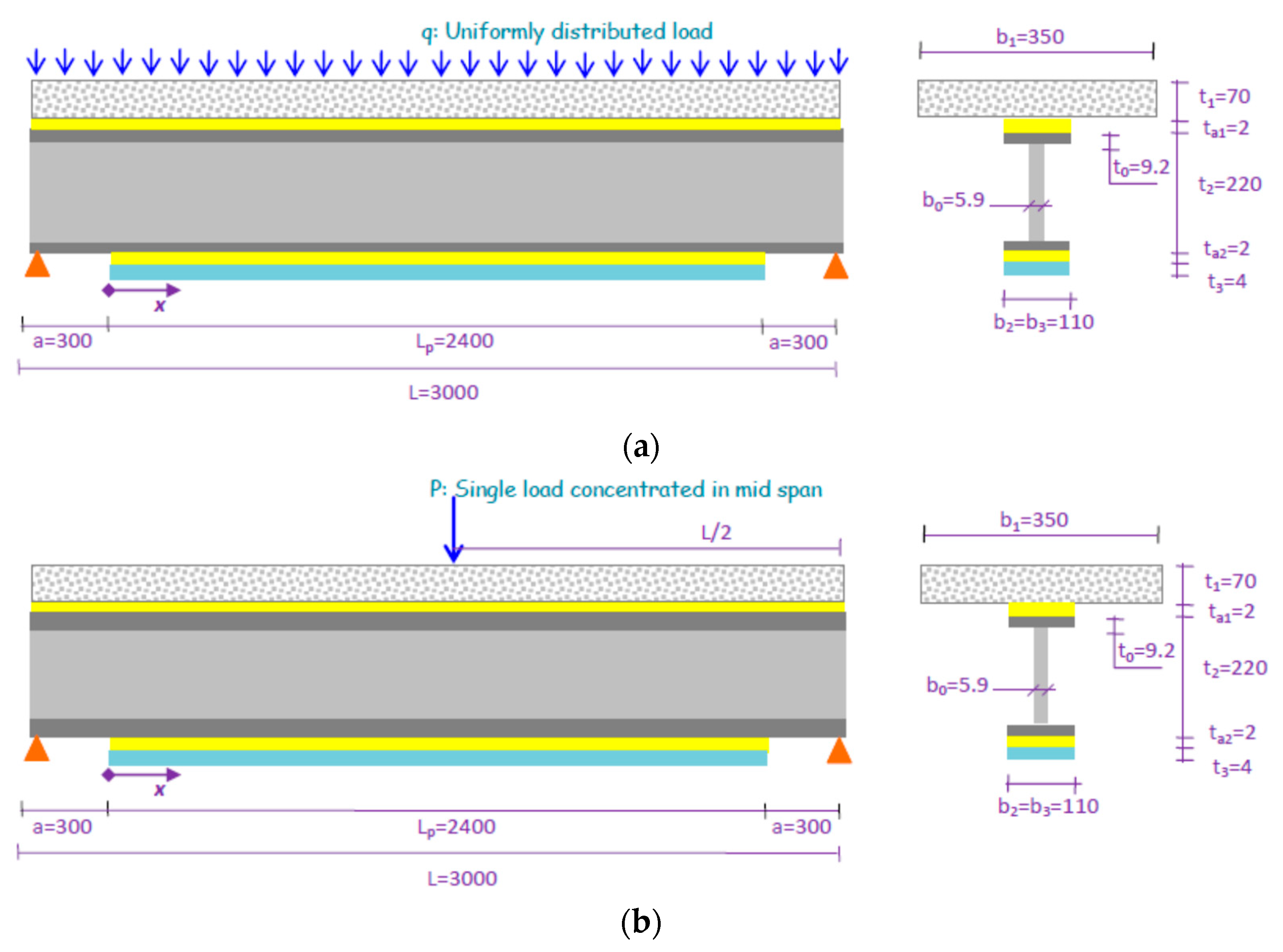
3.1. Material and Geometry Data

The concrete slab and I-steel–concrete beam used in the present study was 3000 mm in length, and the composite plate was 2400 mm in length. The geometrical characteristics and the material properties are given in Figure 10 and

Table 1. Material properties.

Materials		Young’s Modulus (MPa)	Poisson Ratio
Concrete slab	Ordinary concrete	$E_1=\mathrm{36,600}$	${\nu }_1=0.2$
	Siporex concrete	$E_1=2800$	${\nu }_1=0.2$
	Lightweight aggregate concrete	$E_1=\mathrm{10,000}$	${\nu }_1=0.2$
Adhesives	Adhesive 1 (between concrete slab and steel beam)	$E_{a1}=\mathrm{12,300}$	${\nu }_{a1}=0.34$
	Adhesive 2 (between steel beam and composite plate)	$E_{a2}=3500$	${\nu }_{a2}=0.34$
Composites	CFRP	$E_3=\mathrm{165,000}$	${\nu }_3=0.28$
	GFRP	$E_3=\mathrm{65,000}$	${\nu }_3=0.28$
IPE 220 beam	Steel	$E_2=\mathrm{200,000}$	${\nu }_2=0.3$

, respectively.

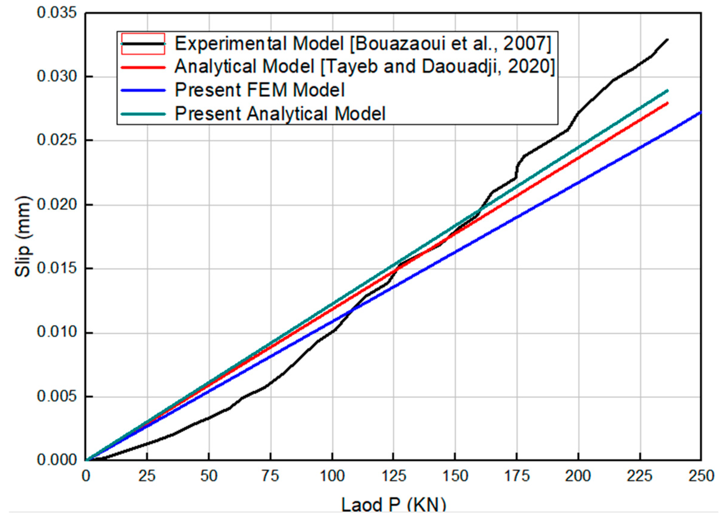
3.2. Validation of the Model by Comparison with Existing Solutions

For the validation of the proposed model, a simply supported composite steel–concrete beam bonded with an adhesive was analyzed. The interfacial slip results of the proposed analytical model were compared with the analytical model of Bensatallah et al. [18] and experimental data from Bouazaoui et al. [19]. The results presented in Figure 11 show good agreement with the published results, confirming the new model’s validity. The study also found that slippage occurs at its maximum when not using the composite beam steel concrete plate and at its minimum when using it. The study emphasizes the importance of using a reinforced composite plate for better slip control.

Furthermore, the finite element simulation method was also compared with the experimental data from Bouazaoui et al. [19], showing good agreement.

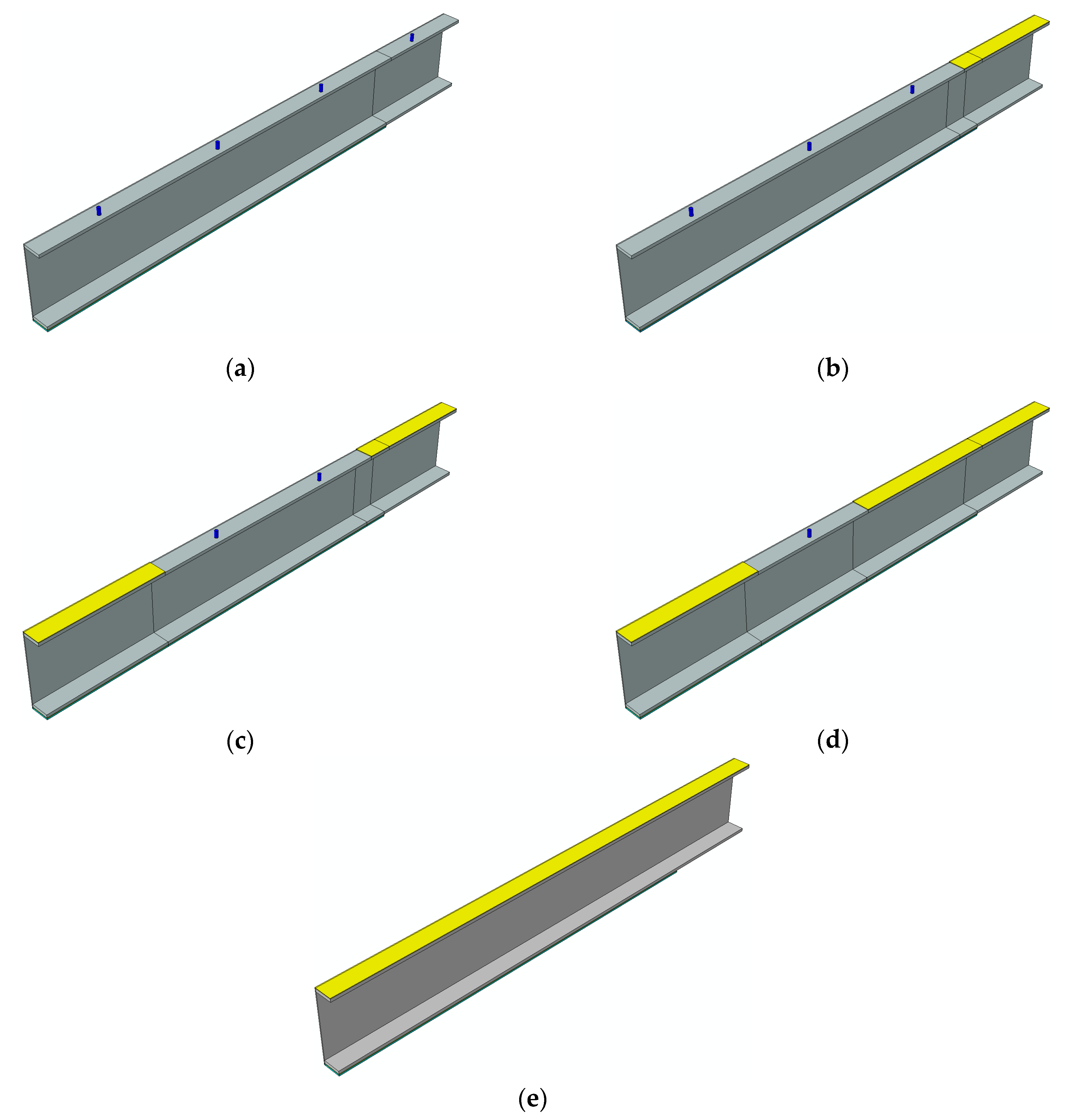
3.3. Finite Element Analysis Results for Hybrid Connection Modes

Figure 12 illustrates the three-dimensional geometry of one-quarter of the composite beam’s cross-section, highlighting the five distinct connection configurations investigated in this study. The corresponding results are presented in Figure 13, which depicts the variation in interfacial slippage between the concrete slab and the steel I–concrete beam under both uniformly distributed loading (UDL) and midspan concentrated loading (CL) for connection modes 1, 3, and 5.

In both loading scenarios, the interfacial slip increases with an increasing external load, which is consistent with the expected response of the composite system. Among the configurations analyzed, mode 1—characterized by the exclusive use of mechanical connectors (shear studs)—exhibits the highest degree of slippage, while mode 5—utilizing adhesive bonding alone—demonstrates the least amount of slippage. This result highlights the superior performance of adhesive joints in promoting effective load transfer and minimizing differential displacement at the steel–concrete interface. Adhesive bonding ensures a continuous and uniform stress distribution across the bonded surface, thereby mitigating localized shear stress concentrations typically associated with discrete mechanical connectors [20,21].

Moreover, an increase in the elastic modulus of the concrete slab leads to a reduction in interfacial slippage across all connection modes. This behavior can be attributed to the enhanced stiffness of the concrete, which limits its deformation under load, thereby reducing relative displacement at the bonded interface.

3.4. Comparison of Analytical Model with Finite Element (FEM) Results

The proposed analytical model is validated by a comparison with a finite element model (FEM) to assess the influence of the concrete’s mechanical properties on the interfacial behavior of composite beams. Specifically, the interface slippage between the concrete slab and the steel I–concrete beam is evaluated for five different connection configurations. The results are summarized in

Table 2. A comparison of the numerical and analytical results for the composite beam reinforced by a CFRP plate under a concentrated load P = 200 kN.

Concrete	Solution	Mode 1	Mode 2	Mode 3	Mode 4	Mode 5
Ordinary	FEM	0.2129	0.0150	0.0149	0.0155	0.0150
	Analytical	0.2091	0.0134	0.0143	0.0150	0.0146
Lightweight aggregate	FEM	0.3286	0.0201	0.0236	0.0223	0.0219
	Analytical	0.3230	0.0190	0.0213	0.0213	0.0211
Siporex	FEM	0.3870	0.0268	0.0336	0.0310	0.0299
	Analytical	0.3833	0.0262	0.0310	0.0304	0.0296

and

Table 3. A comparison of the numerical and analytical results for the composite beam reinforced by a CFRP plate under a uniformly distributed load q = 50 kN/mL.

Concrete	Solution	Mode 1	Mode 2	Mode 3	Mode 4	Mode 5
Ordinary	FEM	0.1298	0.0077	0.0080	0.0080	0.0070
	Analytical	0.1294	0.0075	0.0078	0.0078	0.0063
Lightweight aggregate	FEM	0.1926	0.0099	0.0120	0.0112	0.0100
	Analytical	0.1904	0.0095	0.0119	0.0110	0.0099
Siporex	FEM	0.2253	0.0131	0.0173	0.0155	0.0137
	Analytical	0.2200	0.0129	0.0171	0.0153	0.0129

, corresponding to the cases of midspan concentrated loading and uniformly distributed loading, respectively.

The comparison reveals a strong correlation between the analytical predictions and the numerical simulations, with discrepancies ranging from 0.3% to 10.7%. This close agreement supports the reliability and accuracy of the analytical approach in capturing the fundamental mechanics of interfacial slippage in composite beam systems.

Across all the connection modes, a reduction in the elastic modulus of the concrete results in an increase in the interfacial slippage. This trend reflects the greater deformability of lower-stiffness concrete, which leads to enhanced relative displacement at the interface. In both loading conditions, mode 1—comprising only mechanical shear connectors—exhibits the largest interface slippage, while mode 5—featuring purely adhesive bonding—consistently demonstrates the smallest slippage. These findings underscore the effectiveness of adhesive joints in promoting continuous and efficient stress transfer, thereby reducing interfacial slippage and enhancing the overall composite action of the beam.

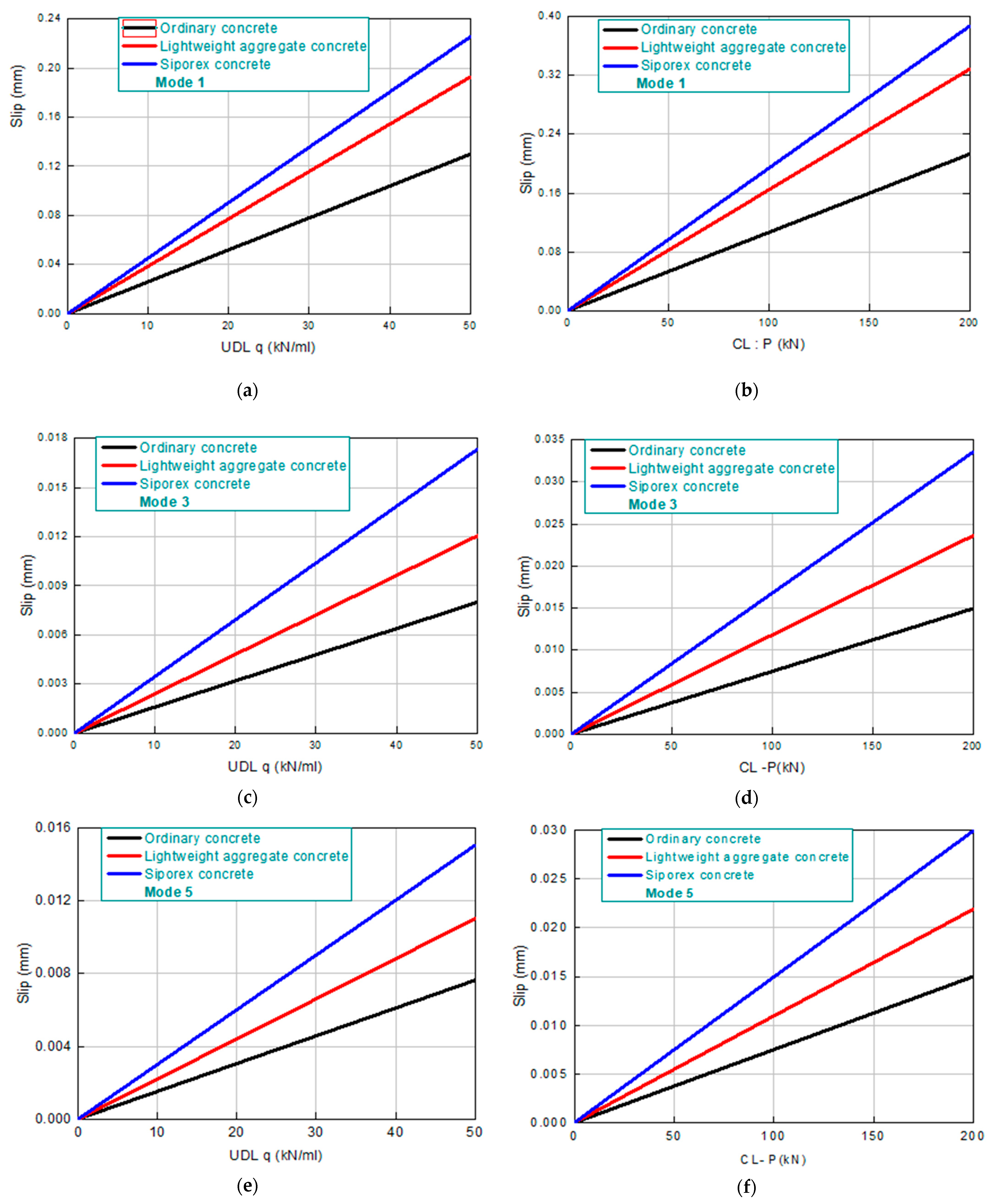
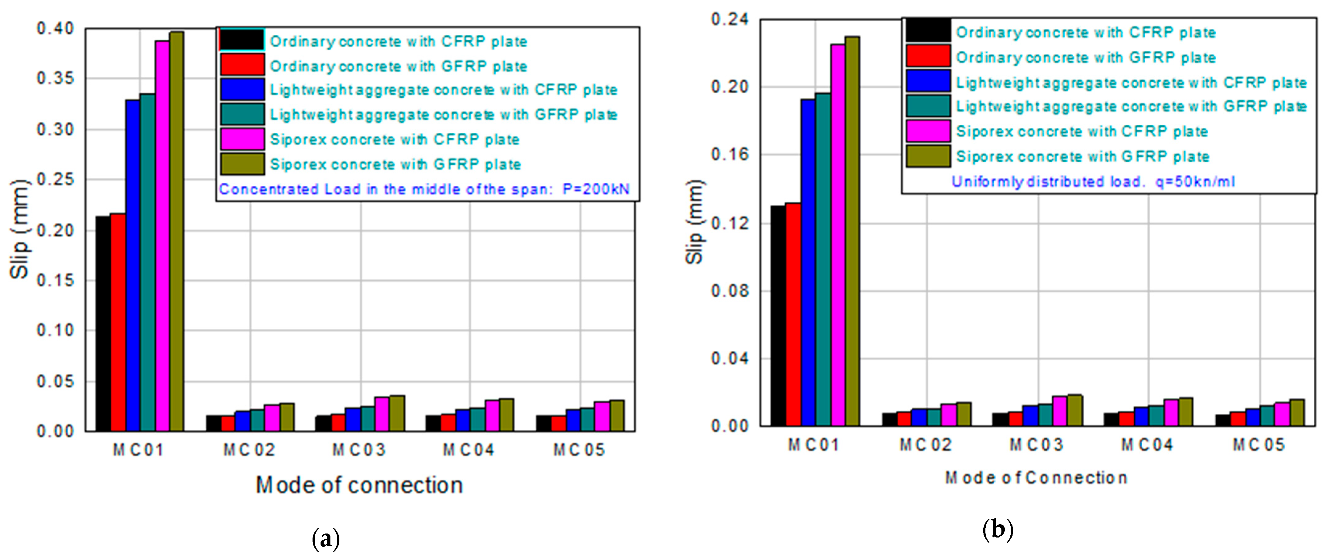
3.5. The Effect of the Type of the Composite Reinforcement and Connection Mode on the Interface Slippage

Figure 14 presents a comparative analysis of the influence of a reinforcement-type polymer—a glass-fiber-reinforced polymer (GFRP) versus carbon-fiber-reinforced polymer (CFRP)—on the interfacial slippage between the concrete slab and the steel I–concrete beam, considering all connection configurations and various concrete material properties.

The results indicate that, across all examined conditions, the composite beam utilizing connection mode 1 (mechanical connectors only) consistently exhibits the highest interfacial slippage, regardless of the reinforcement type. This behavior is attributed to the discrete nature of the shear stud connectors, which can result in localized stress concentrations and less uniform stress transfer compared to continuous bonding systems.

In contrast, composite beams reinforced with CFRP plates consistently demonstrate a lower interfacial slip across all connection modes when compared to their GFRP-reinforced counterparts. This reduction in slip is primarily due to the higher elastic modulus of CFRP, which imparts greater stiffness to the overall composite section. The increased stiffness reduces differential deformation between the concrete slab and the steel beam, thereby enhancing interfacial compatibility and minimizing relative displacement.

These findings underscore the importance of selecting reinforcement materials with appropriate stiffness characteristics to optimize composite action and interfacial performance, particularly in systems utilizing adhesive bonding and hybrid connection strategies.

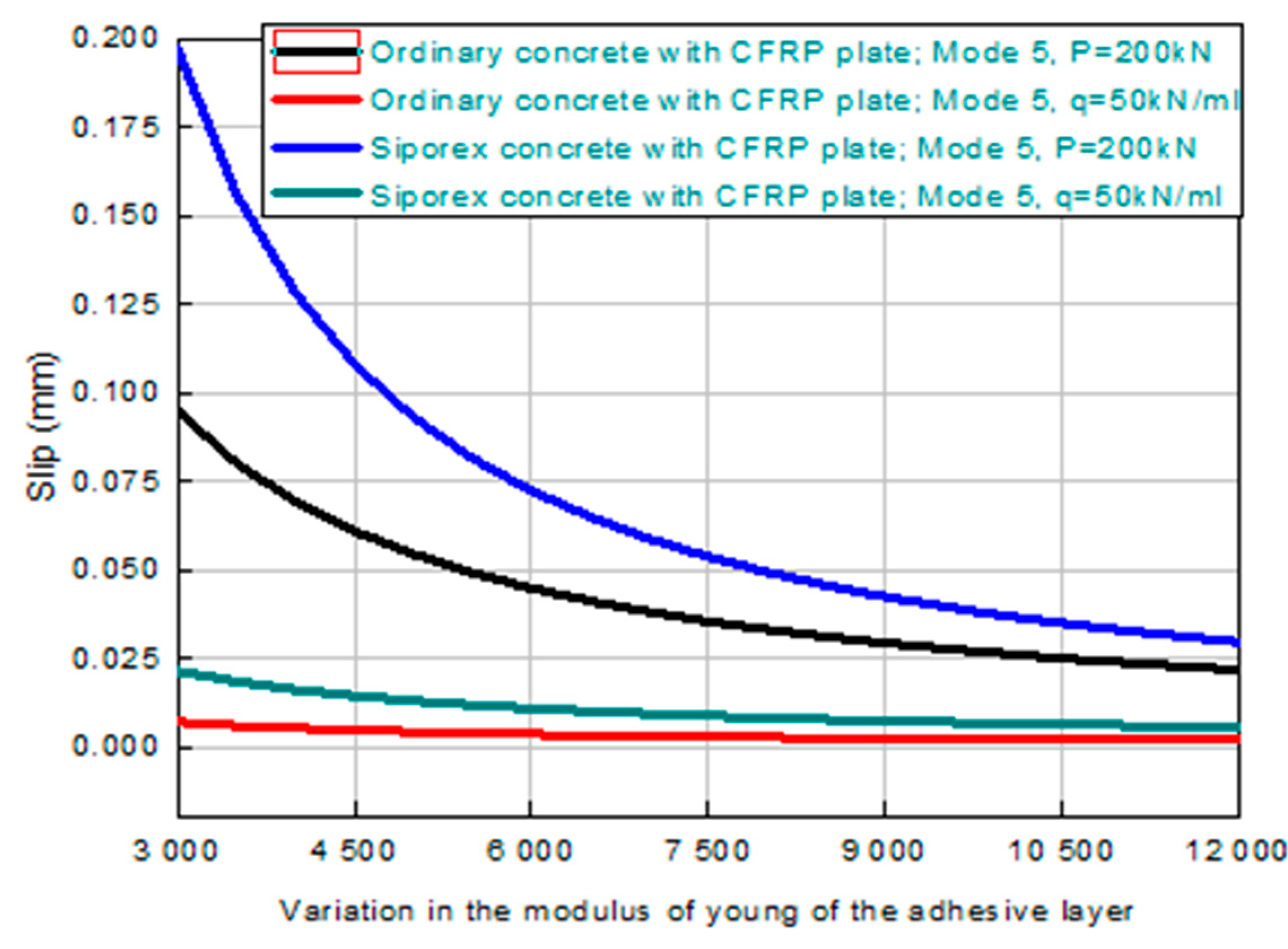
3.6. The Effect of Young’s Modulus for the Adhesive Layer on Interface Slippage

The adhesive layer employed in the composite beam system is modeled as a soft, isotropic material characterized by relatively low stiffness. To evaluate the influence of adhesive stiffness on interfacial behavior, a parametric study was conducted by varying Young’s modulus for the adhesive layer. The results, presented in Figure 15, demonstrate a clear trend: increasing the stiffness of the adhesive significantly reduces the interfacial slip between the concrete slab and the steel I–concrete beam.

This reduction in slippage becomes particularly pronounced when the concrete possesses lower stiffness, as in the case of lightweight cellular concrete (e.g., Siporex), compared to normal-weight concrete. In such scenarios, the flexible nature of both the adhesive and the concrete amplifies the relative displacement at the interface, thereby diminishing the composite action.

While the use of more compliant (lower modulus) adhesives may help alleviate interfacial stress concentrations and accommodate localized deformations, it also compromises the degree of composite action achieved between the externally bonded repair plate and the primary beam structure. This trade-off highlights the critical role of adhesive stiffness in balancing the stress distribution and structural integration within bonded composite systems [20].

4. Conclusions

This study presents an analytical investigation into interface sliding behavior in composite I-steel–concrete beams externally reinforced with fiber-reinforced polymer (FRP) plates.

The main findings and contributions are as follows:

-

The degree of interaction between the steel and concrete, controlled by the shear stiffness of the interface, is critical to the performance of composite systems.

-

Adhesively bonded connections significantly reduce the interface slip compared to mechanical connectors. The adhesive-only configuration (mode 5) consistently showed the least slippage, while mechanical-only connections (mode 1) exhibited the highest slippage, highlighting the effectiveness of continuous bonding in improving stress transfer and reducing shear lag.

-

The proposed closed-form analytical model, based on the nonlinear beam theory, was validated against finite element simulations with discrepancies between 0.3% and 10.7%. The model accommodates various loading conditions and material properties, offering practical utility for structural design.

-

Parametric studies demonstrated that higher adhesive stiffness and CFRP reinforcement reduce interface slippage, especially in beams with low-stiffness concrete (e.g., Siporex), thereby improving composite action and load distribution.

-

The model provides a reliable framework for selecting adhesive properties and reinforcement types, making it a useful tool for the design and retrofitting of bonded composite structures, particularly in structural rehabilitation contexts.

The limitations of the present study are as follows:

-

The analytical model assumes ideal bonding conditions, and the adhesive layer’s stress remains constant throughout the thickness, which may not fully capture localized nonlinearities.

-

Long-term effects, such as creep, shrinkage, and environmental aging, were not considered.

-

This study is limited to static loading conditions and simply supported beam configurations.

Further work should address the following areas:

-

Time-dependent and environmental effects, including temperature sensitivity, adhesive degradation, and durability under moisture.

-

Extended geometries and boundary conditions, including continuous spans, fixed supports, and different cross-section shapes.

References

1. Larrinaga, P.; Garmendia, L.; Piñero, I.; San-José, J.T. Flexural strengthening of low-grade reinforced concrete beams with compatible composite material: Steel Reinforced Grout (SRG). Constr. Build. Mater. 2020, 235, 117790. [Google Scholar] [CrossRef]
2. Cai, M.; Li, W.; Wan, Z.; Sheng, J.; Tan, J.; Ma, C. Cracking control technique for continuous steel-concrete composite girders under negative bending moment. Arch. Civ. Eng. 2023, 69, 239–251. [Google Scholar] [CrossRef]
3. Lin, W.; Lam, H.; Yoda, T. Experimental study on steel–concrete composite twin I-girder bridges. J. Bridge Eng. 2020, 25, 04019129. [Google Scholar] [CrossRef]
4. Benrahou, K.H.; Ameur, M.; Tounsi, A.; Benyoucef, S.; Bedia, E.A. Influence of Adhesive Characteristics on the Interfacial Stress Concentrations in Externally FRP Plated Steel Beams. Compos. Interfaces 2010, 17, 283–300. [Google Scholar] [CrossRef]
5. He, S.; Xu, Y.; Zhong, H.; Mosallam, A.S.; Chen, Z. Investigation on interfacial anti-sliding behavior of high strength steel-UHPC composite beams. Compos. Struct. 2023, 316, 117036. [Google Scholar] [CrossRef]
6. Wang, Y.H.; Yu, J.; Liu, J.P.; Zhou, B.X.; Chen, Y.F. Experimental study on assembled monolithic steel-prestressed concrete composite beam in negative moment. J. Constr. Steel Res. 2020, 167, 105667. [Google Scholar] [CrossRef]
7. Tounsi, A.; Daouadji, T.H.; Benyoucef, S. Interfacial stresses in FRP-plated RC beams: Effect of adherend shear deformations. Int. J. Adhes. Adhes. 2009, 29, 343–351. [Google Scholar] [CrossRef]
8. Henriques, D.; Gonçalves, R.; Sousa, C.; Camotim, D. GBT-based time-dependent analysis of steel-concrete composite beams including shear lag and concrete cracking effects. Thin-Walled Struct. 2020, 150, 106706. [Google Scholar] [CrossRef]
9. Tayeb, B.; Daouadji, T.H.; Abderezak, R.; Tounsi, A. Structural bonding for civil engineering structures: New model of composite I-steel-concrete beam strengthened with CFRP plate. Steel Compos. Struct. 2021, 41, 417–435. [Google Scholar] [CrossRef]
10. Daouadji, T.H.; Abderezak, R.; Rabia, B. Analysis of mechanical performance of continuous steel beams with variable section bonded by a prestressed composite plate. Steel Compos. Struct. 2024, 50, 183–199. [Google Scholar] [CrossRef]
11. Chergui, S.; Daouadji, T.H.; Hamrat, M.; Boulekbache, B.; Bougara, A.; Abbes, B.; Amziane, S. Interfacial stresses in damaged RC beams strengthened by externally bonded prestressed GFRP laminate plate: Analytical and numerical study. Adv. Mater. Res. 2019, 8, 197–217. [Google Scholar] [CrossRef]
12. Rabia, B.; Abderezak, R.; Daouadji, T.H.; Abbes, B.; Belkacem, A.; Abbes, F. Analytical analysis of the interfacial shear stress in RC beams strengthened with prestressed exponentially-varying properties plate. Adv. Mater. Res. 2018, 7, 29. [Google Scholar] [CrossRef]
13. Abderezak, R.; Rabia, B.; Daouadji, T.H.; Abbes, B.; Belkacem, A.; Abbes, F. Elastic analysis of interfacial stresses in prestressed PFGM-RC hybrid beams. Adv. Mater. Res. 2018, 7, 83. [Google Scholar] [CrossRef]
14. Oehlers, D.J.; Coughlan, C.G. The shear stiffness of stud shear connections in composite beams. J. Constr. Steel Res. 1986, 6, 273–284. [Google Scholar] [CrossRef]
15. Silva, A.R.; das Neves, F.D.A.; Junior, J.B.S. Optimization of partially connected composite beams using nonlinear programming. Structures 2020, 25, 743–759. [Google Scholar] [CrossRef]
16. Lavall, A.C.C.; Silva, R.D.; Costa, R.S.; Fakury, R.H. Análise avançada de pórticos de aço conforme as prescrições da ABNT NBR 8800: 2008. Rev. Estrut. Aço 2013, 2, 146–165. [Google Scholar]
17. Simulia. Abaqus Documentations; Dassault Systemes: Vélizy-Villacoublay, France, 2019. [Google Scholar]
18. Tayeb, B.; Daouadji, T.H. Improved analytical solution for slip and interfacial stress in composite steel-concrete beam bonded with an adhesive. Adv. Mater. Res. 2020, 9, 133–153. [Google Scholar] [CrossRef]
19. Bouazaoui, L.; Perrenot, G.; Delmas, Y.; Li, A. Experimental study of bonded steel concrete composite structures. J. Constr. Steel Res. 2007, 63, 1268–1278. [Google Scholar] [CrossRef]
20. Souici, A.; Berthet, J.F.; Li, A.; Rahal, N. Behaviour of both mechanically connected and bonded steel–concrete composite beams. Eng. Struct. 2013, 49, 11–23. [Google Scholar] [CrossRef]
21. Li, A.; Yurtdas, I.; Abbès, B. Creep in steel-concrete composite beams bonded by adhesive and connected by studs. Structures 2025, 74, 108560. [Google Scholar] [CrossRef]
Figure 1. Cross-section view of mechanically connected (existing model) and adhesively bonded (new model) I-steel–concrete composite beam.
Jcs 09 00273 g001
Figure 2. Simply supported composite I-steel–concrete beams reinforced by a composite plate under a uniformly distributed load.
Jcs 09 00273 g002
Figure 3. Simply supported composite I-steel–concrete beams reinforced by a composite plate under a concentrated load in the middle.
Jcs 09 00273 g003
Figure 4. Cross-section of composite I-steel–concrete beams reinforced by composite plate: (a) I-steel–concrete composite beam assembled by connectors; (b) I-steel–concrete composite beam assembled by adhesive.
Jcs 09 00273 g004
Figure 5. Internal forces in the infinitesimal element d x of the of I-steel–concrete beams reinforced by composite material plates.
Jcs 09 00273 g005
Figure 6. Steel beam–concrete slab assembly: hybrid connection type by connectors and/or adhesive: (a) 0% adhesive, (b) 25% adhesive, (c) 50% adhesive, (d) 75% adhesive, (e) 100% adhesive.
Jcs 09 00273 g006
Figure 7. Load definition: (a) concentrated load in midspan; (b) uniformly distributed load.
Jcs 09 00273 g007
Figure 8. Schema of a composite steel–concrete beam with hybrid connection.
Jcs 09 00273 g008
Figure 9. Finite element boundary conditions.
Jcs 09 00273 g009
Figure 10. Geometric characteristics of the composite I-steel–concrete beams reinforced by composite plates: (a) uniformly distributed load; (b) concentrated load in the midspan.
Jcs 09 00273 g010
Figure 11. The comparison of load–slip curves of a simply supported composite steel–concrete beam bonded with an adhesive [18,19].
Jcs 09 00273 g011
Figure 12. Presentation of a quarter of the composite beam section with the five connection modes: (a) mode 1; (b) mode 2; (c) mode 3; (d) mode 4; and (e) mode 5.
Jcs 09 00273 g012
Figure 13. The evolution of the interface sliding between the concrete slab and the I-steel–concrete beam with the following loading modes: (a) mode 1 with UDL; (b) mode 1 with CL; (c) mode 3 with UDL; (d) mode 3 with CL; (e) mode 5 with UDL; and (f) mode 5 with CL.
Jcs 09 00273 g013
Figure 14. A comparison of the interface sliding between the concrete slab and the I-steel–concrete beam with different composite plates used as reinforcement under (a) a concentrated load and (b) a uniformly distributed load.
Jcs 09 00273 g014
Figure 15. The effect of Young’s modulus for the adhesive layer on the interface slip.
Jcs 09 00273 g015