Modeling the Manufacturing Process of Thin-Walled Composite Parts by Vacuum Infusion Using Controlled External Pressures

Abstract

This study considered the molding process of a thin-walled composite structure, imported from a CAD model, with the requirements of the uniformity of the mechanical properties and wall thickness. The developed numerical process model, which includes both the vacuum infusion and post-infusion stages, takes into account the entire complex of processes evolving in a spreading liquid resin, as well as in a porous preform. The controlled process parameters are the temperature and the magnitudes and times of pressure applied to the open surface of the preform and in the vacuum line. The low thickness of the preform walls and the fixation of its inner surface on an open composite mold allow the mechanical part of the problem to be simplified, thus considering only the preform deformation normal to the opened surface, which provides a significant reduction in the simulation time and the ability to effectively optimize the process. The examples associated with the three control modes considered here show that the presented model’s description of the process, with the toolkit for selecting the controlled parameters, eliminates critical situations such as the formation of dry spots, the premature blocking of the vacuum port, or the uneven distribution and insufficient amount of the reinforcing component in the preform. This is due to the appropriately described process dynamics up to the moment of a sharp increase in viscosity and the hardening of the resin. This approach additionally provides access to process parameters that would be inaccessible in a full-scale experiment.

1. Introduction

Towards the end of the last century, when Boeing aircraft first began to use elements of aviation structures—such as ailerons, wings, tail skins, fairings, panels, etc.—made of polymer composites that are much lighter than traditional metal structures, the application and use of these materials began to increase. This trend required deep studies on the destruction of polymer composite structures under tensile, compressive, bending, and shear forces, in addition to both the fatigue and short-term shock loads that can occur during critical flight conditions and forced landings [1]. The listed components of aircraft structures are usually thin-walled parts; therefore, analyses of situations in which they lose local or global stability are of exceptional importance for the safety of the entire aircraft. This circumstance has led to numerous studies investigating problems associated with the crashworthiness and buckling of various composite structures, such as thin-walled multilayer beams [2], columns with different cross-sectional shapes [3], and reinforced panels [4], as well as studies considering ways to increase the strength properties and stability of the aerodynamic shape of such highly loaded structures through design or by using technological methods.

In relatively early works [5,6] that examined the reasons for the low resistance of thin-walled composite structures to concentrated loads, it was noted that such reasons included unwanted deviations from the ideal geometric shape, a change in the thickness of the structure’s walls, and the stiffness of the material under compression. It was later found that the pattern of winding or laying the reinforcement layers has a significant impact on the stability of the structure under various loads, including compressive, torsional, and hydrostatic pressures [7]. Important experimental results, which were convincingly confirmed in references [4,8], showed that the flexural and tensile strength decreases with an increasing laminate thickness, including the very common case of open-hole laminates. These findings show that increasing the thickness of a composite structure is not an effective means of amplifying its strength, especially with respect to impact resistance, although the increased thickness increases its weight. Below are some design techniques that can improve the strength properties of a thin-walled composite structure and reduce the influence of negative factors.

As presented in early works [6,9], it was convincingly shown that ensuring the required strength and stability characteristics of critical composite structures in practice through their rational design, while accommodating for the constraints on the weight, the properties of existing components, and the technologies available, is a very difficult problem that requires expert decision making. Among such solutions, one should note the solution of increasing the mechanical stiffness of the polymer matrix by adding reinforcing particles; optimizing the specific volume of the reinforcing component, which varies within the body of the structure; optimizing the winding and laying angles (fiber volume fraction); and changing the laying order of the reinforcing layers [7,9,10,11], as well as optimizing the variation in the distribution thickness along the surface of the structure [11], taking into account the nature of the ultimate loads and the zones of their application. However, when considering the results of these studies, which proposed effective but difficult-to-implement solutions, it is important to understand that their main goal was to eliminate the shortcomings of the technologies used for the production of large-sized composite structures, such as local decreases in the specific fiber volume fraction, variations in wall thickness, and the presence of empty pores not filled with resin. These disadvantages are inherent in the vast majority of technologies used for the production of large-sized, thin-walled composite structures, which are formed, as a rule, in open molds by injecting liquid resin into a dry preform, often using a vacuum. Such shortcomings are caused, first of all, by the complexity of the liquid resin front propagation, due to the complexity of the preform geometry, the presence of “open windows” (large empty internal regions) in it, the uneven distribution of pressure inside the pores of the preform filled with liquid resin, and the continuous change in the kinetic and rheological state of the resin during its movement [12,13,14].

The optimization of the traditional processes used with resin injection into a dry preform, such as resin transfer molding (RTM) or some type of vacuum-assisted resin transfer molding (VARTM, VAP), in order to eliminate these disadvantages is usually carried out using the rational resin injection gates and the exit vent location [15] through pressure and temperature control [13]. In practice, such a quasi-optimal acceptable solution is found using either the trial-and-error method or continuously improved computer modeling tools [13,14,15]. The most advanced of these modeling systems provides the correct reconstruction of the resin propagation front; all thermal effects, including the exotherm of the curing thermoset resin; the change in the viscosity, taking into account the change in the permeability of the porous preform during its deformation; and heuristic approaches to speed up and increase the efficiency of determining the optimal solutions [13].

Despite significant progress in the development of methods for modeling and optimizing traditional processes for the RTM and VAP molding of thin-walled composite structures, a number of works have proposed technical solutions that provide the technologist with additional degrees of freedom to eliminate the quality assurance problems discussed above. The authors of [16] proposed the so-called pulsed vacuum infusion process, which is implemented through the use of an external rigid chamber placed on top of a standard VI assembly, providing an increase in the elastic modulus and flexural strength by 9% and 24%, respectively, compared to traditional composites obtained by the method of vacuum infusion. The disadvantage of this method relates to the ribbed surface of the external hard bag, which is copied by the surface of the infused structure. This feature limits the scope of this method’s application to structures whose surface smoothness is not required.

Reference [17] shows that the use of a post-infusion dwell for approximately 1.5 h at temperatures of about 80 °C and constant pressure ensures a reduced porosity and a greater resistance of the manufactured samples to the peak load during impact tests. However, the application of the method in practice requires careful preliminary research, taking into account the geometry of the molded structure, the compressibility and permeability of the preform, the thermokinetics of polymerization, and the viscosity of the resin used.

An analysis of a large number of works devoted to improving the quality of layered, polymer composite, thin-walled structures produced by infusion methods showed that the most effective and fairly general solution to the problem is the technology of controlled post-infusion external pressure proposed in [18,19]. Experimental studies on various scenarios for post-infusion treatment using controlled pressures of small rectangular samples have reliably confirmed the effectiveness of equalizing the post-infusion pore pressure, thus reducing the preform thickness and increasing the fiber volume fraction. As a result, the strength properties were significantly improved. Implementing the process under production conditions requires placing the molded preform in a closed chamber with a controlled pressure and temperature, and it also requires the ability to regulate the pressure in the vacuum line. This is possible in an autoclave with sufficient dimensions.

This technology, like traditional vacuum infusion, requires optimization for the design of the process layout and modes. However, such optimization is significantly more complex than in the case of traditional vacuum infusion processes due to the larger number of design variables. This set of additional design variables includes the steady-state values, rates, and moments of change in external compressive and vacuum pressures after filling the preform with resin. The correct reconstruction of the actual state of the preform at the post-infusion stage requires solving a system of Navier–Cauchy equations [20], coupled with equations of pore pressure diffusion, heat transfer, and the kinetics/diffusion/convection of the degree of cure α. In 3D cases, this is a very computationally labor-intensive task. However, the thin-walled nature of the infusion composite structure and the relatively slow evolution of the process at the post-infusion stage make it possible to significantly reduce the computational complexity of the modeling problem by describing the deformations of the fiber preform based on the shell concept. Fixing the inner surface of a thin preform on an open mold allows its in-plane deformations to be neglected and normal deformations to be considered the main ones, which affects the porosity, the permeability, and ultimately, the dynamics of the spreading of liquid resin. The effectiveness of this concept is substantiated using examples of the analytical [21] and finite element [13] modeling of filling simple thin-walled preforms with liquid resin. This study considered the vacuum-infusion process of a real 3D thin-walled composite structure. In particular, it included the formulation of the modeling problem and its finite element implementation, which required the preliminary refinement of the imported CAD model of the structure to be manufactured, numerical modeling of three different process scenarios, and an analysis and discussion of the results.

2. Numerical Modeling of the Combined Vacuum Infusion and Post-Infusion Molding

The prototype of the modeled part was a thin-walled rotorcraft part with double curvature, a large overall size of 0.613 m, and a smaller one of 0.305 m. The part was made of unidirectional tape with SYT45-12K carbon fibers (Zhongfu Shenying Carbon Fiber Co., Ltd., Lianyungang, China), 8 layers of which were impregnated with low-temperature curing epoxy resin, EDT-10 (Condor Oil, Ltd., Calgary, AB, Canada), with the hardener content recommended by the manufacturer. The architecture of the laid laminate [0°;90°;45°;−45°;−45°;45°;90°;0°] ensured its symmetry, balance, and transverse isotropy in the cured state with a raw preform thickness of 3 mm. The open mold on which the carbon tape layers were laid out was extended by 50 mm around the perimeter of the infusion blank. It was made from similar recycled carbon fibers by hot pressing and milling to a thickness of 6 mm. This ensured the satisfactory thermal conductivity of its material, which was assumed to be isotropic in the modeling.

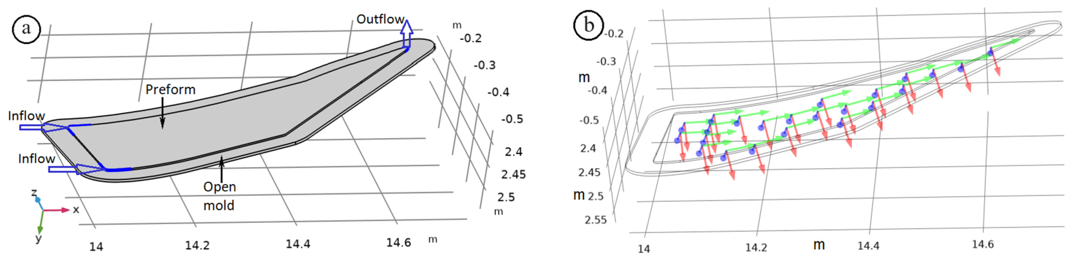
When formulating the system of governing equations for the problem, the following assumptions were made. The modeling object was a porous preform that was considered as an elastic frame laid face down on an open mold made of polymerized carbon fiber plastic. The back, outer side of the preform, which was covered with a thin-walled vacuum bag, was exposed to atmospheric and controlled external pressure. The surfaces of the preform were isolated with the exception of the resin gates (inflow) and the vacuum line (outflow), which were in fixed positions and connected to the preform in narrow areas of its side surface (see Figure 1a). In the initial state, with a constant pore pressure in the body of the preform, its material was assumed to be homogeneous, and all its parameters, including the elastic and thermal properties, porosity, and permeability, were assumed to be constant. To describe the anisotropy of the material in the region with curved boundaries, local curvilinear coordinate systems were introduced, as presented in Figure 1b.

Taking into account the finite element (FE) method for solving the forward-modeling problem in the Comsol Multiphysics 6.1 software, the system of governing equations included the following:

• A phase field equation specified in the preform and describing the resin front propagation as follows:

$$\partial \varphi /\partial t+u\cdot \nabla \varphi =\nabla \cdot \gamma \nabla G,$$

(1)

where the dependent variable $\varphi \in [-1;1]$ determines the local resin filling V_r according to $V_r=\left(\varphi +1\right)/2\in [0;1]$, G is the chemical potential, γ is the phase mobility, and u is the superficial velocity of the liquid resin.

• The convection/diffusion/kinetics in Equation (2) for the spatiotemporal evolution of the degree of cure α as follows:

$$\partial \alpha /\partial t-\left([K]/\mu \right)\cdot \nabla p\cdot \nabla \alpha -\nabla \cdot \left(c_{\alpha }\nabla \alpha \right)=F\left(\alpha ,T\right),$$

(2)

which combines the three most important phenomena in a moving thermoset resin—the cure kinetics; diffusion, the coefficient of which (c_α) depends on the kinetic state of the resin; and the convective movement of the degree of cure α during the flow of the resin. In this equation, [K] is the permeability tensor of the porous medium, adopted in diagonal form for a transversely isotropic preform material, and the source term F(α,T) ≡ dα/dt, which describes the evolution of α with time and temperature and which obeys the autocatalytic equation, also taking into account the significant reduction in the cure rate when the reaction becomes diffusion-controlled towards the end of curing [22,23].

$$F\left(\alpha ,T\right)=A{\displaystyle \frac{w\exp \left(-E_1/RT\right)+\exp \left(-E_2/RT\right)\cdot {\alpha }^m}{1+\exp \left(\left(\alpha -0.75\right)/0.25\right)}}{\left(1-\alpha \right)}^n,$$

(3)

where R is the universal gas constant and T is the temperature in Kelvin. The activation energies E₁ and E₂, the weight coefficients A and w, and the reaction orders m and n determine the cure rate of epoxy resin polymerization. All these parameters of the selected thermosetting resin were found experimentally using a Netzsch 200 F3 Maia (Netzsch Group, Selb, Germany) differential scanning calorimeter, with the subsequent identification of their values using a genetic algorithm [24]. The modified empirical dependence of the diffusion coefficient c_α on the degree of cure α was taken in the following form:

$$c_{\alpha }=5\cdot {10}^{-7}{\displaystyle \frac{1+\exp \left((\alpha -0.35)/0.25\right)}{1+\exp \left((\alpha -0.85)/0.06\right)}}{\mathrm{m}}^2/\mathrm{s}$$

(4)

The solution to Equation (2) allows us to determine the intensity of the exothermal heat Q_exo released per unit volume of cured resin as follows:

$$Q_{exo}=Q_{tot}{\rho }_r\left(1-V_f\right)\cdot V_r\cdot \partial \alpha /\partial t,$$

(5)

where Q_tot is the total amount of exothermal heat released during the curing per unit mass of resin; ρr is its mass density; and V_f is the fiber volume fraction in a porous medium, which is related to the porosity $\phi$ by the relationship $V_f=1-\phi$.

• Darcy’s equation was used for the body of the preform to relate the velocity u of the gas–fluid mixture with the pore pressure gradient $\nabla p$ as follows:

$$\left\{\begin{array}{c}{\displaystyle \frac{\partial }{\partial t}}\left(\phi {\rho }_{gr}\right)+\nabla \cdot \left({\rho }_{gr}u\right)=Q_m\\ u=-{\displaystyle \frac{\left[K\right]}{{\mu }_{gr}}}\nabla p\end{array}\right.,$$

(6.1)

where

$${\rho }_{gr}={\rho }_r{V}_r+(1-V_r){\rho }_g,$$

(6.2)

$${\mu }_{gr}={\mu }_r{V}_r+{\mu }_g\left(1-V_r\right)$$

(6.3)

are the mass density and dynamic viscosity of the moving gas–resin mixture, depending on the filling of the pores with liquid resin V_r, and they are determined by the mixing rule. Q_m is the source/sink of the mass taken equal to zero. All the diagonal components of the permeability tensor [K] in (2) and (6.1) satisfy the Kozeny–Karman model, expressed as follows [20]:

$$Q_{exo}=Q_{tot}{\rho }_r\left(1-V_f\right)\cdot V_r\cdot \partial \alpha /\partial t,$$

(6.4)

and the minimum permeability parameter ${\tilde{k}}_n$ normal to the preform surface is taken to be 4 times less than the parameter ${\tilde{k}}_t$ in the direction of the tangent plane ${\tilde{k}}_t=4\cdot {\tilde{k}}_n=2\cdot {10}^{-10}$m². The values of the relative fiber volume fraction V_f and porosity ϕ depend on the compressive pressure $p_{comp}(r)=p^{appl}-p(r)$ and on the filling of the preform with liquid resin V_r according to the following mixing rule:

$$V_f=1-\phi =V_r\cdot V_f^{wet}+\left(1-V_r\right)\cdot V_f^{dry},$$

(6.5)

where the empirical relationships are as follows:

$$V_f=V_{f\_\min }+b^{dry,wet}\cdot a\cosh \left(1+p_{comp}/a^{dry,wet}\right),$$

(6.6)

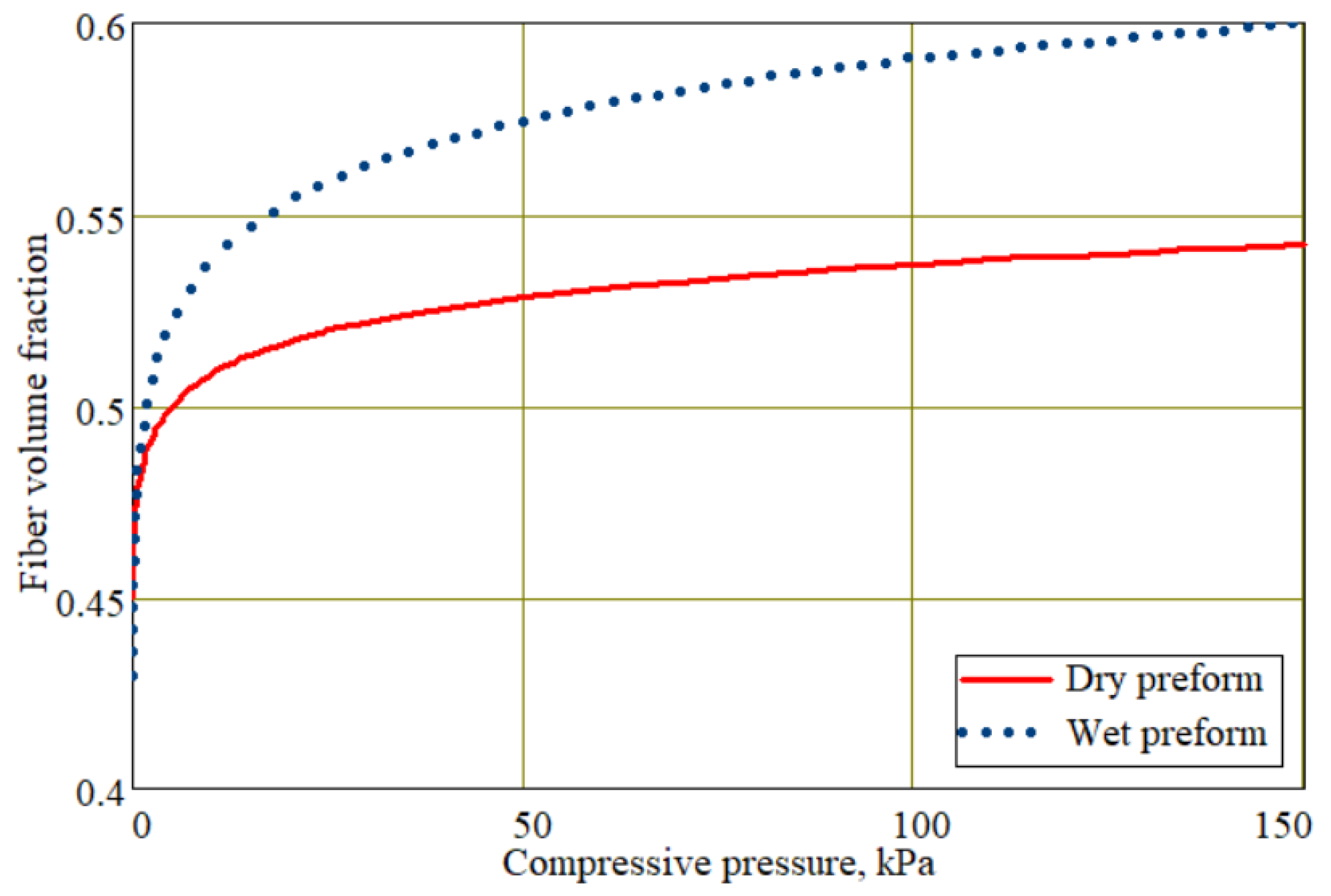
and they describe the compressibility of dry and fully wetted preforms (see Figure 2).

For the change in the thermosetting resin viscosity μ_f during the curing process, we proposed a modified model that takes into account the initial viscosity ${\mu }_f^0$ of the resin before it is injected into the preform, as well as the dependence of the degree of curing on the temperature and time as follows [13]:

$${\mu }_f\left(T,\alpha ,t\right)={\mu }_f^0(T^{in})\cdot \exp \left({\upsilon }_1\cdot (T(t)-T^{in})+{\upsilon }_2\cdot \alpha (T,t)\right),$$

(6.7)

where the initial value of the resin viscosity ${\mu }_f^0(T^{in})$ and both model parameters υ₁ and υ₁ were found with the use of an Anton Paar MCR 72/92 (Anton Paar GmbH, Graz, Austria) rheometer.

The initial viscosity and temperature dependences of both coefficients ${\upsilon }_1,{\upsilon }_2$ included in Equation (6.7) were determined experimentally using viscometry.

• The heat transfer equation was defined in the preform as follows:

$${\rho }_{pr}{C}_{pr}\partial T/\partial T+\nabla \cdot \left(-k_{pr}\nabla T\right)=Q_{exo},$$

(7.1)

where the thermal properties of the preform, ρ_pr, C_pr, and k_pr, were determined using the following mixing rule:

$${\rho }_{pr}={\rho }_f\cdot (1-\phi )+\phi \cdot {\rho }_{gr},$$

(7.2)

$$C_{pr}={\rho }_f(1-\phi )\cdot c_f+\phi \cdot {\rho }_{gr}{c}_{gr},$$

(7.3)

$$k_{pr}={\left({\displaystyle \frac{\phi }{\left(k_r{V}_r+k_g(1-V_r)\right)}}+{\displaystyle \frac{(1-\phi )}{k_f}}\right)}^{-1}$$

(7.4)

For an open CFRP mold, the heat transfer equation was the same, but with unchanged properties ρ_m, _Cm, and k_m [25].

The most important initial and boundary conditions for these equations were the following.

For the phase field (Equation (1)), the initial and boundary conditions were as follows:

$$\begin{array}{l}{\varphi }_{{\mathsf{\Omega }}_{pr}}\left(0\right)=-1\Rightarrow V_r\left(0\right)=0;\\ \begin{array}{cc}\left\{\begin{array}{c}{\varphi }^{inl}\left(t\right)=1\Rightarrow V_r^{inl}\left(t\right)=1;\\ {\varphi }^{out}\left(t\right)=-1\Rightarrow V_r^{out}\left(t\right)=0;\end{array}\right.& \forall t,\end{array}\end{array}$$

(8)

where the subscript Ω_pr denotes the body of the preform and the superscripts ^inl and ^out denote the boundaries of the resin gates (inlets) and vacuum vent (outlet), respectively.

For Equation (2), which describes the change in the degree of cure of the resin, the following was true:

$${\alpha }_{{\mathsf{\Omega }}_{pr}}\left(0\right)=0.$$

(9.1)

On all closed boundaries, the zero-flux condition was accepted as follows:

$$n\cdot \left(c_{\alpha }\nabla \alpha \right)=0,$$

(9.2)

and at the boundaries of the resin gates, the Dirichlet condition was used as follows:

$${\alpha }^{inl}\left(t\right)={\alpha }_{inj}\left(T^{in}\right),$$

(9.3)

where the degree of cure α_inj of the injected resin is constant and depends only on its temperature T_in. The boundary condition of free α-flux $S_{\alpha }^{out}$ through the vacuum vent was as follows:

$$S_{\alpha }^{out}=n\cdot \left(c_{\alpha }\nabla \alpha \right)\left(n\cdot u\right),$$

(9.4)

where u is the fluid flow vector through the vacuum vent and n is the unit normal vector to the boundary.

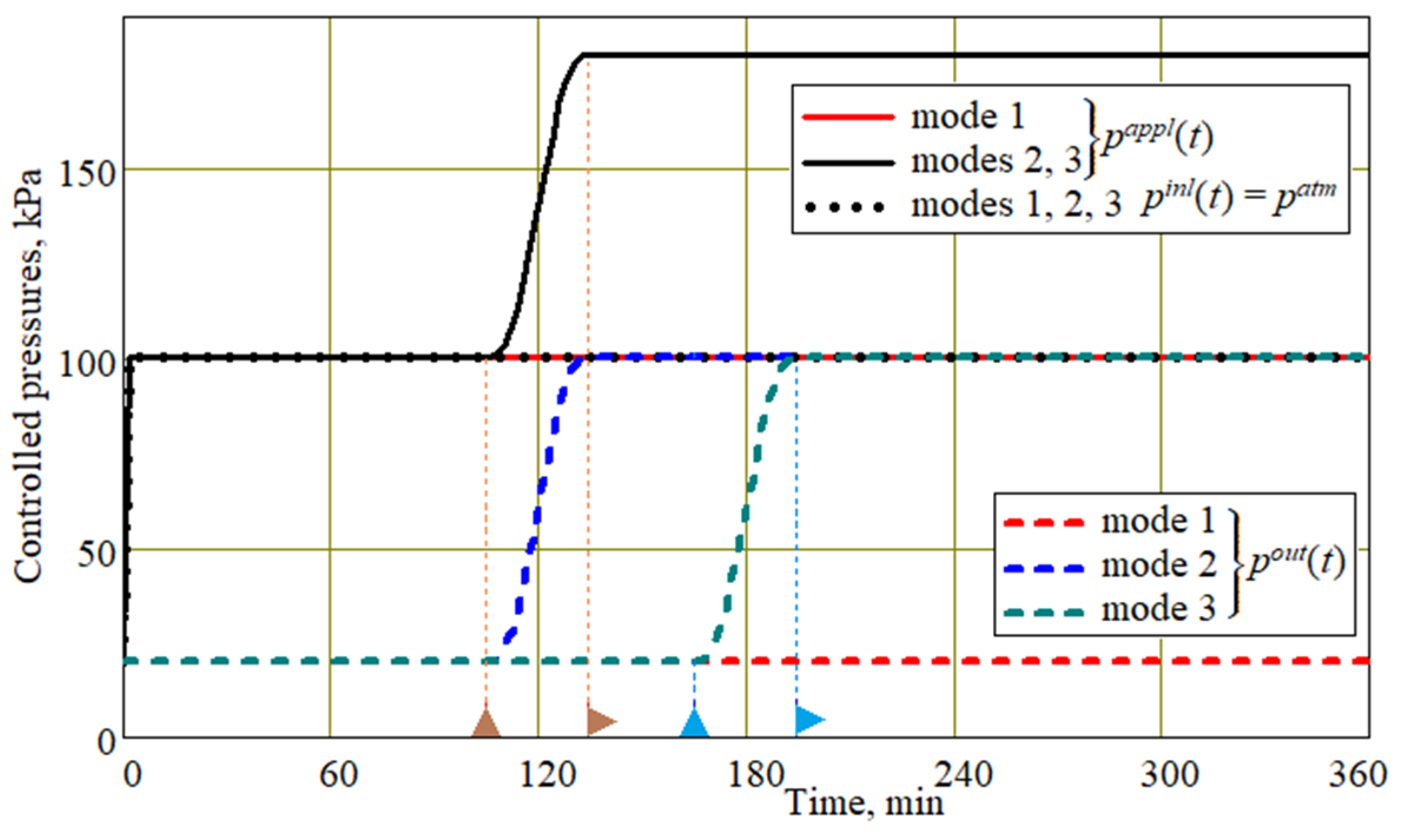
The initial value of the pore pressure p(0) in the preform was equal to the vacuum pressure p(0) = p_vac, and the evolving pore pressure p (see Equation (6)) was controlled by the pressures in the resin gate, p_inl(t) = p_atm. This was unchanging and equal to the atmospheric pressure p_atm, the pressure in the vacuum vent p_out(t), and the external pressure p_appl(t) applied to the outer open surface of the preform. This article discusses three infusion process modes, which differ in their laws of control by the external compressive pressure and the pressure in the vacuum line. These modes, which are presented as time dependences in Figure 3, are intended to equalize the pore pressure along the entire preform and ensure that its thickness remains constant after resin solidification. The moment of the beginning of the p_out(t) and p_inl(t) = p_atm pressure equalization depends on the duration of the preform filling with resin, i.e., on its cure rate and on the preform’s shape and dimensions. A premature increase in p_out(t) can result in the formation of voids in the vicinity of the vacuum port, while a late increase in this pressure can lead to the non-uniformity of pore pressure, the formation of internal stresses, and areas of different thicknesses.

The first mode studied (mode 1) is a conventional vacuum infusion process, during which the external pressure and the pressure in the vacuum port are maintained constant as follows:

$$\left\{\begin{array}{c}{p}^{appl}\left(t\right)=p^{atm}=100 kPa\\ p^{out}\left(t\right)=p_{in}^{out}=20 kPa\end{array}\right..$$

(10.1)

The second mode (mode 2) is characterized by the presence of a post-infusion stage, which begins after the preform is approximately 95% filled with resin, after which the external pressure and the pressure in the vacuum vent simultaneously and smoothly increase from the initials to some stationary values as follows:

$$\left\{\begin{array}{c}{p}^{appl}\left(t\right)=p^{atm}+p^{add}\cdot H\left(t_{start}^{appl},\Delta t_{start},t\right)\\ p^{out}\left(t\right)=p_{in}^{out}+(p^{atm}-p_{in}^{out})\cdot H\left(t_{start}^{appl},\Delta t_{start},t\right)\end{array}\right..$$

(10.2)

where $t_{start}^{appl}$ is the moment that the pressure rise begins, $\Delta t_{start}$ is the duration of the pressure rise to the final value, and H is the smoothed Heaviside function.

The third mode (mode 3) differs from mode 2 by the moment that the outlet pressure rise begins, $t_{start}^{out}=t_{start}^{appl}+t_{lag}$, as follows:

$$p^{out}\left(t\right)=p_{in}^{out}+(p^{atm}-p_{in}^{out})\cdot H\left(t_{start}^{out},\Delta t_{start},t\right),$$

(10.3)

where t_lag is taken as 60 min. The time instants when the external and outlet pressures change are denoted in Figure 3 by the little triangle signs as follows: the start–stop of the rise in the external pressure are shown by , and similarly, the start–stop of the rise in the outlet pressure are shown by .

The initial temperature value T_in for both bodies (the injecting preform and the mold) was assumed to be 75 °C. Liquid resin was injected into the resin gates at the same temperature, while all the open surfaces of the preform and mold were exposed to a convective air flow heated to 80 °C according to the following law:

$$T_{conv}\left(t\right)=T_{in}+\Delta T\cdot {\tanh }^2\left(t/\tau \right),$$

(11)

where ΔT = 5 K and τ = 120 min.

The intensity of convective heat flow depends on the heat transfer coefficient, taken as being equal to 10 W/(m²∙K). The intensity of the internal source of exothermal heat in the preform, depending on the kinetic state of the resin (which itself is a function of time, temperature, and position in the preform), is determined by Relation (5). All the thermophysical constants of the mold material, as well as the properties of the preform, depending on the porosity, resin filling, and viscosity, were determined similarly to our previous work [13].

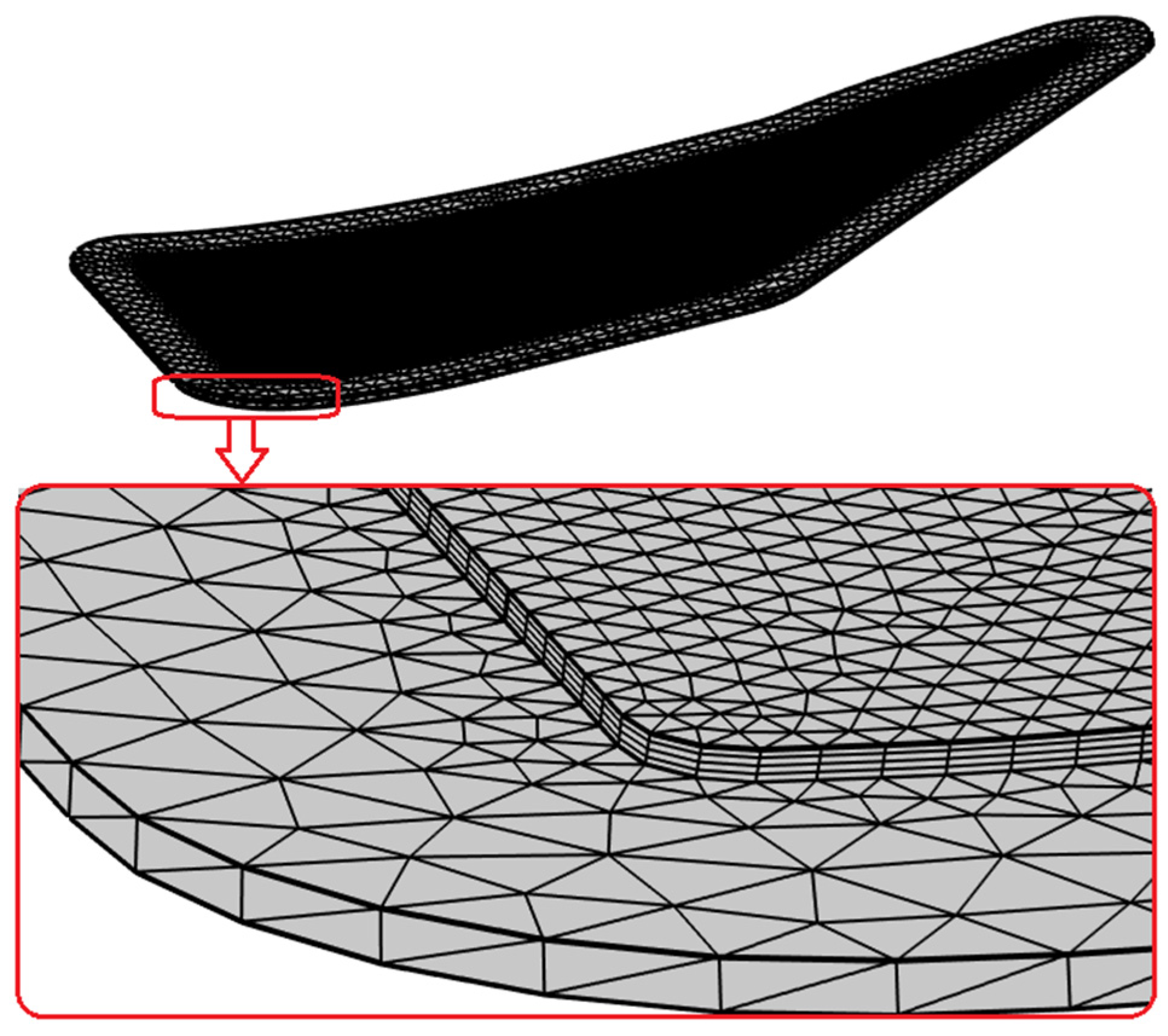
The formulated problem was numerically implemented in the Comsol Multiphysics 6.1 FE package. The original geometry of the molded part was processed in the NX CAD1899 version modeling software tool in order to remove the joints of the front surface pieces, smooth it, and then create open-mold geometry. In the CAD model of the part, the areas of resin injection gates and vacuum ports were highlighted (see Figure 1a). The geometry of the model after FE meshing is presented in Figure 4. The FE preform mesh included 4 swept layers of triangular elements with side dimensions of 5.5–6.0 mm, and the open mold mesh included position-dependent tetrahedral elements with a maximum increase in the side dimensions not exceeding 1.5.

During the infusion process, the outer surface of the preform is subjected to significant pressure to press it down into the surface of the mold and eliminate the possibility of any displacements or deformation in the tangent plane.

It is important to note that the compressibility diagrams of the preform under study in Figure 2 were obtained experimentally under the same conditions; that is, the value of the fiber volume fraction can be determined with great accuracy by using these diagrams if the compressive stress is known. This stress is equal to the difference between the external compressive p_appl and the pore pressure p in the preform [20].

This assumption allowed us to use the found distributions of resin filling V_r and pore pressure p at each step of integration in Equations (1), (2), (6.1), and (7.1) to determine the spatial distribution of the fiber volume fraction V_f according to Formulas (6.5) and (6.6). Then, the dependence of the preform thickness h on V_f was determined from the following simple relation:

$$h=h_{in}\cdot V_{f,in}/V_f$$

(12)

where h_in and V_f,in are the local thickness and the fiber volume fraction of the uncompressed preform, respectively.

After constructing a curvilinear coordinate system and initializing the initial state of the system, a transient analysis of the process was carried out until the moment of stopping after 6 h (21,600 s) of simulated time. With the maximum time step set to 120 s, the calculation time averaged ~45 min. To analyze the simulation results, the average, maximum, and minimum probes of the main process parameters were formulated in the volume of domains and at their boundaries.

3. Results and Discussion

Before discussing the results of the numerical experiments, it should be noted that the considered type of vacuum infusion technology is oriented specifically for the production of thin-walled composite structures; therefore, its main objectives are a uniform distribution and the maximum achievable fiber volume fraction, and consequently, wall thickness in the formed part. However, in manufacturing environments, the process’ performance and reliability are also very important. The concept of technology reliability assumes minimal variability in quality indicators, with small changes in the properties of the components and control actions. In addition, the evolution of the process depends on several interrelated phenomena as follows: the kinetics of the resin cure, changes in the resin viscosity, the velocity of its propagation from the pore pressure gradient, and the permeability of the porous preform frame, which in turn depends on the filling of the resin. These phenomena, which were identified during modeling; their relationships; and their impact on the process objectives under consideration are of the greatest interest and are discussed below.

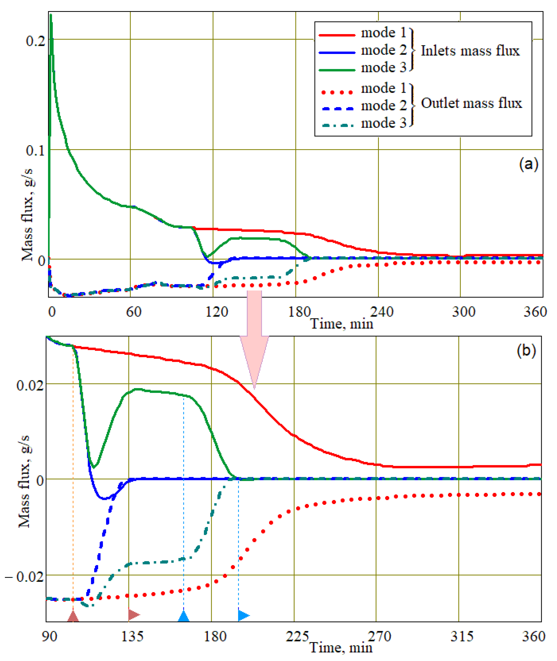
As shown in Figure 5, the time dependences of the resin mass fluxes through the injection gates and the gas–liquid mixture through the vacuum vent demonstrated an initially rapid but slowing decrease in the magnitude of these fluxes with time before the start of applying external compressive pressure to the preform. Up to this point, the behavior of mass fluxes for all three considered modes was the same. Note that, after approximately two hours of resin injection in the first mode (usually implemented using vacuum infusion), the mass inflow and outflow became almost identical. This is quite understandable, since by this moment, the preform was nearly completely filled with liquid resin. After three hours of the process (see Figure 5b), the value of the mass fluxes in mode 1 decreased even more and asymptotically approached zero, which can be mainly explained by a significant increase in the viscosity of the resin, as shown in Figure 6. This figure demonstrates an increase in the viscosity of the resin, which was caused by some growth in the temperature due to the generated exothermal heat Q_exo at the maximum increase in the resin cure rate ∂α/∂t (see Formulas (5) and (7.1)). At such relatively low temperatures, the solidification of the resin under study did not occur, which made it possible to complete the filling of the preform with resin.

With a simultaneous increase in the external pressure on the preform’s opened surface and in its vacuum port on mode 2, the inlet and outlet mass fluxes were sharply reduced, and the flow of mass through the injecting port even changed direction for a short time. That is, the resin was pushed outward through the injection ports. An increase in the pressure in the vacuum vent for mode 3, which occurred with some temporary lag from the beginning of growth in the injection gates, also led to the almost complete stop of the resin movement.

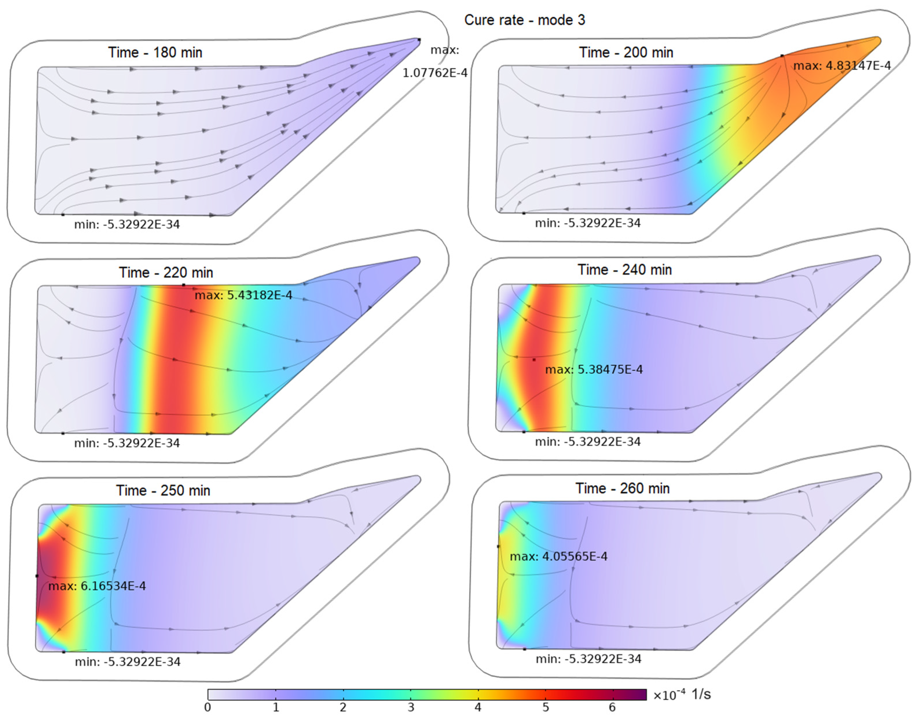
As we can see, an increase in viscosity in modes 2 and 3 occurred earlier than in mode 1 due to the early increase in the degree of resin cure and temperature. This phenomenon was due to the cessation of the arrival of fresh resin with a negligible degree of curing from the injection gates. This stage of the process is illustrated with 3D screenshots that combine the spatial distribution of the cure rates associated with the exothermal heat intensity and the resin velocity streamlines (see Figure 7). They show that, during the period under consideration, the movement of the resin practically stopped, and the region of intense heat generation moved from the outlet to the region of the resin input and then disappeared. In this case, although the viscosity of the resin increased sharply, its average value was such that the resin still retained fluidity. This fact illustrates the influence of the resin propagation dynamics on thermokinetic processes.

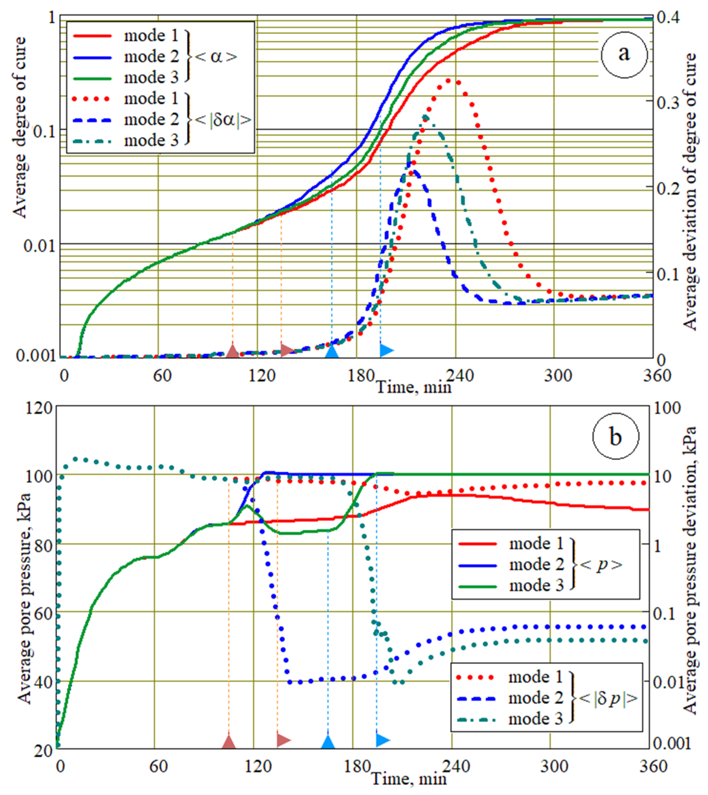
As shown in Figure 8a, the time dependences of the average degree of resin cure <α> and their deviation <|δα|> in the volume of the preform demonstrated a faster stabilization of the degree of curing after a sharp decrease in the volume of resin entering the preform from the injection gates and the almost complete stop of its movement in modes 2 and 3.

The dynamics of liquid resin propagation in the preform were largely determined by its permeability and pore pressure gradient (see Formula (6.1)), which both depended on the pore pressure distribution in the preform. Figure 8b shows the time dependences of the average value <p> and the dispersion <|δp|> of the pore pressure in the volume of the preform under different control modes.

The plots of the average degree of cure <α> and pore pressure dispersion <|δp|> in Figure 8 for mode 1 demonstrate that, when <α> approaches 1, i.e., at the completion stage of the resin cure, <|δp|> is equal near 10 kPa, which leads to significant changes in both the fiber volume fraction <δV_f> and the wall thickness <δh> deviations in the finished part. In contrast, the achieved deviation of <δV_f > in modes 2 and 3 was more than 100 times smaller and occurred approximately 2 h earlier, when the resin still had sufficient fluidity. It is this feature of the method of applying external pressure that ensured the uniform distribution of V_f and h throughout the body of the molded part, which is necessary to achieve the best criteria for structural strength.

Note that the achieved stable value of the pore pressure p in modes 2 and 3 reached 100 kPa, becoming equal to the atmospheric pressure p_atm. Despite the applied external pressure of 180 kPa, the pore pressure p did not exceed p_atm. 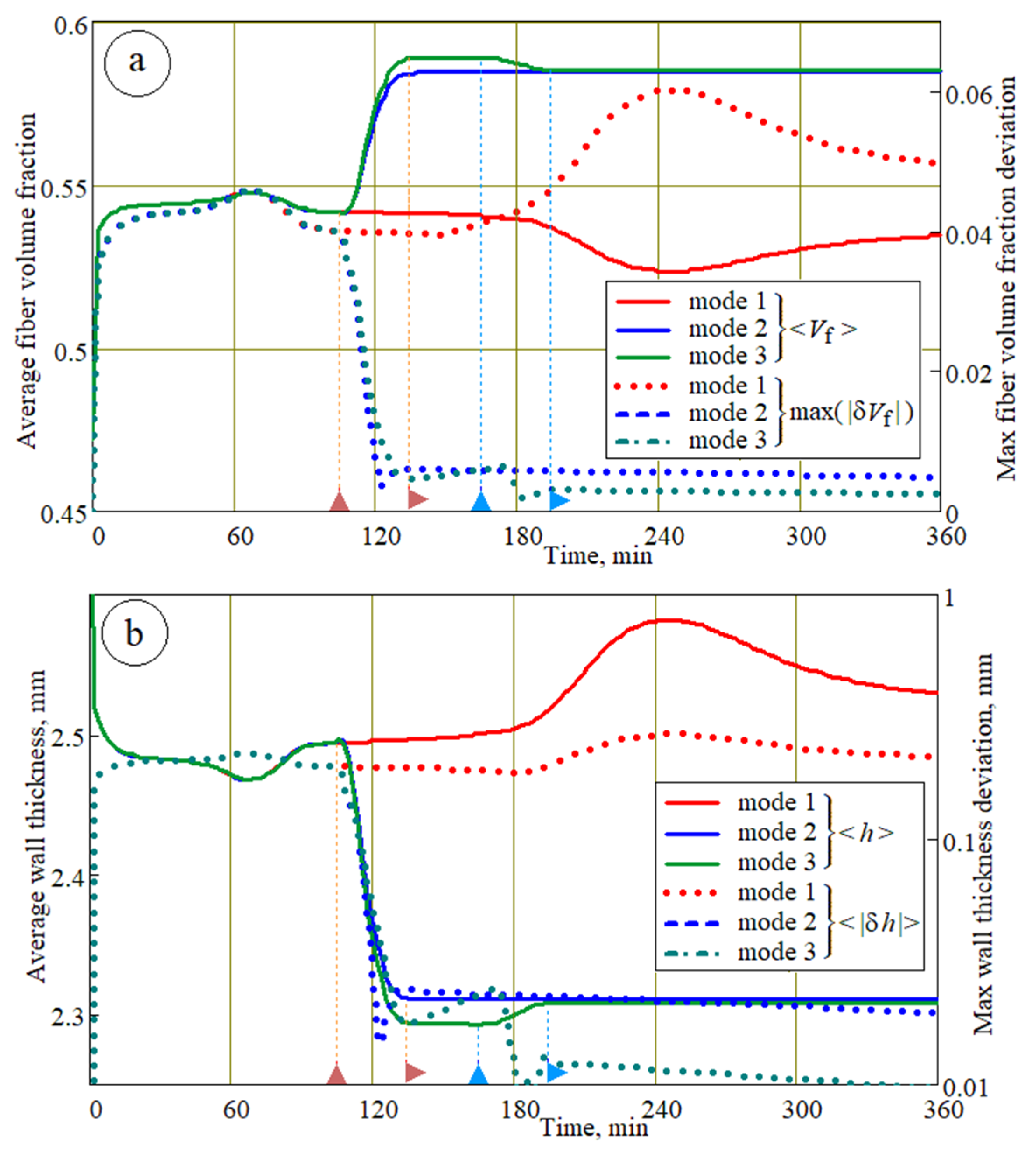This was due to the fact that, after the pressure p_out in the vacuum vent finished increasing and stabilized, the pressure in the open vacuum and injection ports became equal to p_atm. In this case, the compressive pressure in the preform was about 80 kPa, which ensured the significant compressive deformation of the porous frame, an increase in the fiber volume fraction (see Figure 9a), and a decrease in the wall thickness (see Figure 9b). The comparison of plots in Figure 9a shows that the best result was achieved with mode 3, while the conventional vacuum infusion process produced an average fiber volume fraction of approximately 10% less at its 20-fold greater variation. This conclusion was confirmed by Figure 9b, which shows changes in the thickness of the preform walls during the implementation of all the molding modes analyzed.

The evolution of the fiber volume fraction for the three studied modes is clearly illustrated in Figure 10a–c, which shows the combined 3D screenshots of the resin flow streamlines and V_f across several moments in time. In addition, they show resin fill levels of 0.5 and 0.9 with solid yellow and red lines, respectively. The first three screenshots in Figure 10a for the time points of 30 min, 60 min, and 104 min correspond to the three modes, that is, before applying controlled pressures to the preform. The remaining three screenshots correspond only to mode 1, while the screenshots in Figure 10b,c correspond to modes 2 and 3, when additional external pressure p_appl was applied to the preform surface.

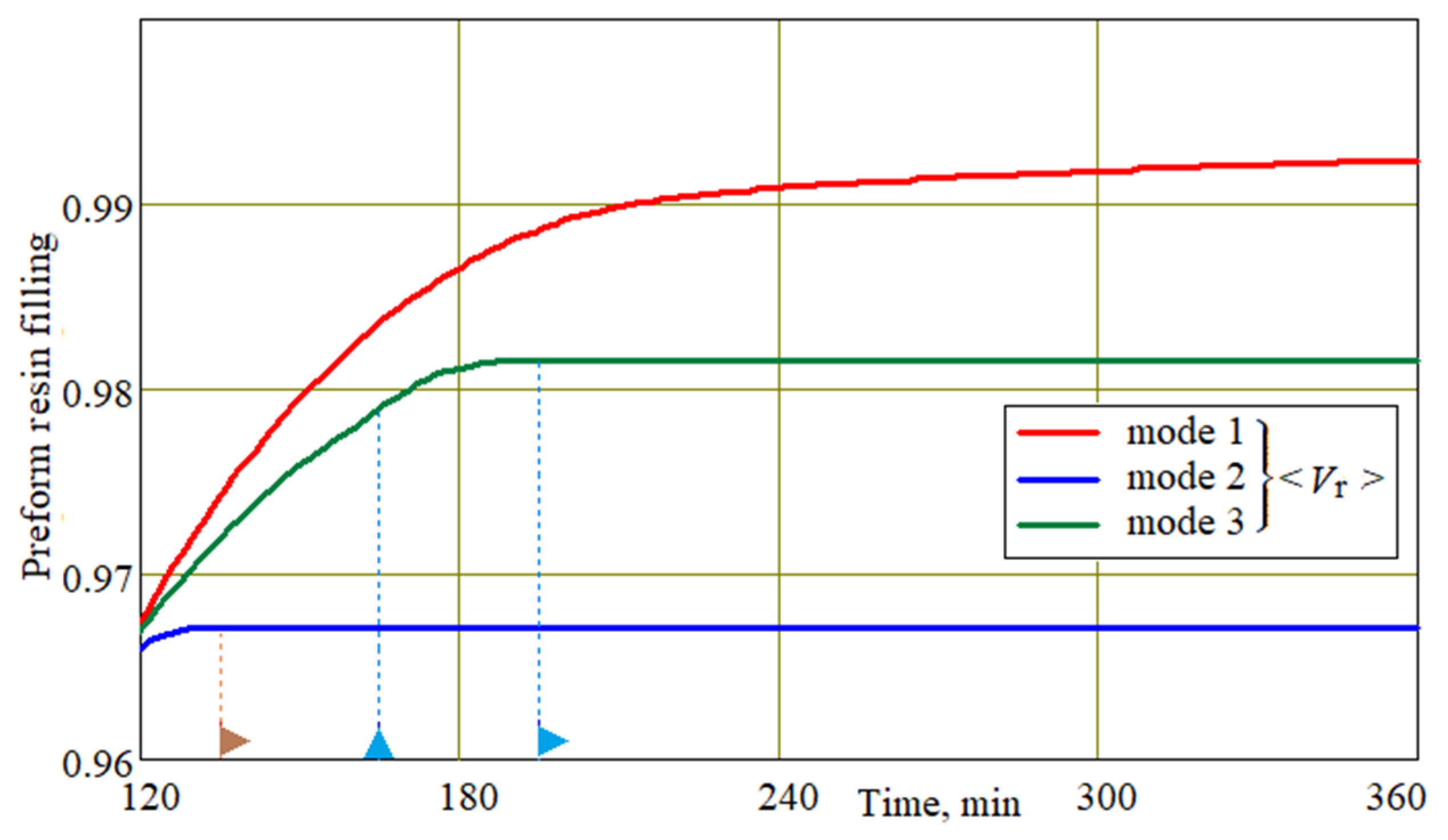
Comparing these three sets of screenshots confirmed the benefit of applying external controlling pressure to achieve a more uniform distribution of the fiber volume fraction, but it also revealed the undesirable effect associated with some slowdown in the preform’s resin filling. A lower speed of filling preforms with resin was characteristic of mode 2, in which the external p_appl and pressure p_out in the vacuum port increased synchronously. In this mode, at 240 min, the filling level Vr = 0.9 was still quite far from the outlet vent; in mode 1, this filling level had long since gone beyond the preform.

The obtained result is further confirmed by the time diagrams in Figure 11, showing the V_r level for all the studied modes. This drawback can be explained by the fact that an increase in the outlet pressure p_out at constant pressures in the injection gates led to a decrease in the pore pressure gradient and, as a consequence, to a decrease in the resin velocity.

Outside the range of issues considered, two additional means of improving the target criteria and the reliability of vacuum infusion processes remain. The first of these can be a very effective means of eliminating the disadvantage associated with the slowing of resin flow when equalizing the pore pressure in the preform. This solution, studied experimentally and published in [18,19], offers an alternative scenario for implementing dynamic pressure control. It is similar to the one discussed here, but differs in the fact that, as the external compressive pressure increases, the injection port closes. Obviously, in this case, two resin flows moving in opposite directions cannot be formed, but there will be only one flow directed towards the outlet port. In this case, the pore pressure will no longer asymptotically tend to atmospheric pressure and will be regulated by changing the compressive pressure.

The advisability of using another means is due to the fact that, upon equalizing the pore pressure to the atmospheric pressure and minimizing its variation in the preform, it is desirable to completely finalize the resin cure under these conditions. This is possible by placing the entire process system in either an autoclave or a sealed chamber using the controlled infrared irradiation of the preform [26]. Both of these promising solutions will be examined in future research.

It is important to note that the presented results of the numerical simulations quantitatively and qualitatively coincide with the data of previously measured experimental observations. These are, first of all, the filling of the preform with resin (visually) and the resin flow passing through the injectors and the vacuum vent, as measured by flow meters. However, the simulations provide an understanding of the dynamics of spatiotemporal distributions, such as the degree of cure and rheology of the resin, the pore pressure, its gradient, and the fiber volume fraction, which are inaccessible for experimental measurement. These simulations, using the experimentally determined characteristics of the components, provide valid and very clear information up to the onset of a sharp increase in the degree of curing and solidification of the resin.

4. Conclusions

1. This study, which focused on the production of thin-walled composite structures with increased requirements for strength and geometric accuracy using the vacuum infusion method, presents a mathematical model of the process that takes into account the dynamics of liquid resin propagation in the porous preform, an evolving resin rheology, thermal phenomena, and the effect of controlled external pressures applied to ensure the maximum level of reinforcement with minimal variability and a constant wall thickness of the molded structure. The possibility of a significant improvement in these process parameters using controlled pressure in the vacuum port, proposed in [18,19] and confirmed experimentally by the authors of this article, encountered difficulties in the rational choice of time characteristics for controlling this pressure under production conditions. The post-infusion stage of the molding process, which was repeatedly observed in experiments, revealed a number of problems with their rational choice. Among them was the formation of regions of the preform unfilled with resin in the immediate vicinity of the vacuum port due to the early start of increasing the pressure in it to the atmospheric pressure. On the other hand, a late increase in vacuum pressure at the stage when the degree of cure and viscosity of the thermosetting resin increase sharply leads to the vacuum port becoming blocked, as well as the occurrence of “dry spots” and the uneven distribution of pore pressure in the preform body, disrupting the uniformity of thickness and generating undesirable residual stresses with subsequent warping. The forward problem of modeling solved in this work aimed to create a reliable tool suitable for the rational selection of process modes when molding composite structures of various sizes and shapes.

2. Using the example of a thin-walled aircraft structure, the geometry of which was imported from a CAD model, simulations of the vacuum infusion molding process on an open composite mold were carried out under three modes, differing in the moments of application and the magnitude of the external pressures to the open surface of the preform and in the vacuum vent. The results of the numerical experiments presented in this study confirmed the possibility of achieving the target process objectives that significantly exceed those when using conventional vacuum infusion processes, and they also made it possible to determine the influence of controllable factors and methods for their rational choice when developing production technology.

3. It was shown that the capabilities of the developed software tool and the studied patterns inherent in the complex multiphysics process under consideration make it possible to exclude the occurrence of critical situations if there is a sufficient set of experimental data on the properties of the components. This ensures the highest achievable process quality and productivity. It should be noted that, when using nanoparticles as an additional filler in the production of polymer composites, the developed software can be effectively used if appropriate experimental data are available on all components of the molded composite.

4. The forward problem considered is a part of the multi-objective optimization problem. Its use for optimization purposes in practice is possible either by assigning each quality criterion its own weight, based on the importance of the criterion for the operational characteristic (geometric accuracy, porosity, and bearing capacity) and constructing a global quality criterion, or by using the Pareto approach and decision making. The solution to such problems as applied to specific structures with the required design and operational parameters is the subject of our ongoing and future research.