Boundary Characteristic Bernstein Polynomials Based Solution for Free Vibration of Euler Nanobeams

Abstract

This paper is concerned with the free vibration problem of nanobeams based on Euler–Bernoulli beam theory. The governing equations for the vibration of Euler nanobeams are considered based on Eringen’s nonlocal elasticity theory. In this investigation, computationally efficient Bernstein polynomials have been used as shape functions in the Rayleigh-Ritz method. It is worth mentioning that Bernstein polynomials make the computation efficient to obtain the frequency parameters. Different classical boundary conditions are considered to address the titled problem. Convergence of frequency parameters is also tested by increasing the number of Bernstein polynomials in the simulation. Further, comparison studies of the results with existing literature are done after fixing the number of polynomials required from the said convergence study. This shows the efficacy and powerfulness of the method. The novelty of using the Bernstein polynomials is addressed in detail and solutions obtained by this method provide a better representation of the vibration behavior of Euler nanobeams.

1. Introduction

Nanomaterials are those for which a single unit is sized between 1 and 100 nm. In the present time, nanomaterials are used in many sectors, e.g., information technology, solar panels, optical and electronics, medical and health care applications, etc. Small-scale effects and the atomic forces are admissible to get the acceptable accuracy from nanoresonators [1] and nanoactuators [2]. Research on nanobeams show that the classical beam theories could not capture the small-scale effect in the mechanical properties of nanobeams [3]. The ignorance of small-scale effect may cause a completely incorrect solution in nano-designing fields and hence it causes improper designs. Wang and Hu [4] showed that classical beam theories could not able to predict the decrement of phase velocities of wave propagations in a carbon nanotube when the wavenumber is so large that the microstructure has a significant influence on the flexural wave dispersion. In this regard, the nonlocal elasticity theory has been introduced by Eringen [5]. Various beam theories including Euler–Bernoulli and Timoshenko beam theories have been reformulated using the nonlocal differential constitutive relations by Reddy [6]. The author derived the equation of motion considering the nonlocal theories and also provided the corresponding analytical solution of bending, buckling, and vibration of beams.

The nonlocal elasticity has been used for the analysis of nanostructures like nanobeams, nanoplates, nanorings, carbon nanotubes, etc., because forces between atoms and internal length scale are considered in this theory [7,8,9]. A nonlocal beam theory to investigate the bending, buckling and free vibration of nanobeams was proposed by Aydogdu [10]. Wang et al. [11] solved the free vibration problem of Euler–Bernoulli nanobeams by analytical methods. Authors have compared the frequency parameters for different scaling effect parameters and for various boundary conditions such as, Simply Supported (S-S), Clamped-Simply Supported (C-S), Clamped-Clamped (C-C) and Cantilever beams.

Phadikar and Pradhan [12] solved equations for bending, buckling, and vibration of Euler nanobeams by finite element analysis. The authors computed results for nanobeams with various boundary conditions viz. Simply Supported, Clamped, and Free. Few authors have used different methods viz. the finite element method [13], Chebyshev polynomials in the Rayleigh-Ritz method [14], meshless method [15], differential quadrature method [16], and differential transform method [17] to study vibration analysis of nanostructures. Further, free vibration of Euler nanobeams has been investigated by using the Rayleigh-Ritz method with boundary characteristic orthogonal polynomials with different boundary conditions [18,19,20,21,22]. Fernandez-Saez J et al. [23] solved the bending of Eule–Bernoulli beam considering the Eringen’s integral formulation. Authors formulate the problem of the static bending of Euler–Bernoulli beam using the nonlocal integral equation.

In the present paper, we have used Bernstein polynomials in the Rayleigh-Ritz method to analyze the free vibration of Euler nanobeams. The Bernstein polynomials are helpful for implementation in computer programs since it satisfies various recurrence relations for differentiation as well as integration [24]. In this work, we study the vibration analysis of Euler nanobeams with different boundary conditions (S-S, C-S, C-C). The numerical results are compared with previous records and we found a very good agreement. Furthermore, this computational procedure takes less time than the previous methods by using Bernstein polynomials. Here we have used Simple Bernstein polynomials (SBPs) and further, we also orthogonalize the SBPs by using the Gram–Schmidt orthogonalization process to get Orthogonal Bernstein polynomials (OBPs). The OBPs are also used to find the frequency parameters of Euler nanobeams. The advantage of using Bernstein polynomials has been about less computation time compared to other polynomials as shape functions. Further, the orthogonalized Bernstein polynomials have also advantage compared to simple Bernstein polynomials as in the former case the generalized eigenvalue problem transforms to standard eigenvalue problem thereby reducing computational complexity. Further, a new convergence theorem has been developed here to show the theoretical convergence of displacement function with respect to the said polynomials.

2. Theoretical Formulation

The strain displacement relation based on Euler–Bernoulli beam theory is given by,

$${\epsilon }_{xx}=-z\frac{d^{2}w}{d{x}^2}$$

(1)

where $x$ is the longitudinal coordinate measured from the left end of the beam, ${\epsilon }_{xx}$ is the normal strain, z is the coordinate measured from the mid-plane of the beam, and $w$ is the transverse displacement.

Let $U$ be the strain energy, which is given by Reference [18]

$$U=\frac{1}{2}{\displaystyle \underset{0}{\overset{L}{\int }}{\displaystyle \underset{A}{\int }{\sigma }_{xx}}{\epsilon }_{xx}dAdx}$$

(2)

where ${\sigma }_{xx}$ is the normal stress, $A$ is the area of the cross-section of the beam, and L be the length of the beam.

The bending moment is given by,

$$M={\displaystyle \underset{A}{\int }{\sigma }_{xx}zdA}$$

(3)

We use Equations (1) and (3) in Equation (2), then the maximum strain energy may be expressed as [15]

$$U_{\max }=-\frac{1}{2}{\displaystyle \underset{0}{\overset{L}{\int }}M\frac{d^{2}w}{d{x}^2}}dx$$

(4)

Assuming the free harmonic motion, the maximum kinetic energy is obtained as [18]

$$T_{\max }=\frac{1}{2}{\displaystyle \underset{0}{\overset{L}{\int }}\rho A{\omega }^2{w}^{2}dx}$$

(5)

where $\omega$ is the circular frequency of the vibration and $\rho$ be the mass density of the material of the beam.

The governing equation of motion is given by Reference [25] (we consider the harmonic vibration and effects of rotary inertia is neglected)

$$\frac{d^{2}M}{d{x}^2}=-\rho A{\omega }^{2}w$$

(6)

For an elastic material in the one-dimensional case, Eringen’s nonlocal constitutive relation may be written as [10]

$${\sigma }_{xx}-{(e_{0}a)}^2\frac{d^2{\sigma }_{xx}}{d{x}^2}=E{\epsilon }_{xx}$$

(7)

where E is Young’s modulus, $e_{0}a$ is the scale coefficient that incorporates the small-scale effect. Here, a is the internal characteristic length (e.g., lattice parameter, C-C bond length, and granular distance) and $e_0$ is a constant appropriate to each material. The magnitude of $e_0$ may be determined from experiments or approximated by matching the dispersion curves of plane waves with those of atomic lattice dynamics.

Now multiplying Equation (7) by $zdA$ and integrating over the area $A$, we obtain

$$M-{(e_{0}a)}^2\frac{d^{2}M}{d{x}^2}=-EI\frac{d^{2}w}{d{x}^2}$$

(8)

where $I$ is the second moment of area.

Substituting Equation (6) in Equation (8), we get,

$$M=-EI\frac{d^{2}w}{d{x}^2}-{(e_{0}a)}^2\rho A{\omega }^{2}w$$

(9)

3. Solution Methodology

The vibration equation of Euler nanobeam has been solved by using Rayleigh-Ritz method, with Bernstein polynomials as the basis function. For this, we introduce the following non-dimensional terms

$$X=\frac{x}{L}$$

$$W=\frac{w}{L}$$

$$\alpha =\frac{e_{0}a}{L}=\mathrm{scaling\; effect\; parameter}$$

Bernstein Based Rayleigh-Ritz Method

Here, the displacement function is assumed as

$$W(X)={\displaystyle \sum _{i=0}^n{c}_i{\varphi }_i}$$

(10)

where $c_i$’s are the unknowns (to be determined) and n is the order of the approximation.

The shape functions ${\varphi }_i$’s are chosen as

$${\varphi }_i(X)={\eta }_b{B}_{i,n}(X)$$

(11)

where $B_{i,n}(X)$’s are the Bernstein polynomials [21]

$$B_{i,n}(X)={(}_i^n)X^i{(1-X)}^{n-i}$$

(12)

where ${(}_i^n)=\frac{n!}{i!.(n-i)!}$; $i=0,1,\dots n$. And ${\eta }_b$ is the non-dimensional boundary polynomial for nanobeam with different boundary conditions which may be written as

$${\eta }_b=X^p{(1-X)}^q$$

(13)

where p and q take the values of 0, 1, or 2 according to Free, Simply Supported, or Clamped, respectively. Thus, we can easily handle the boundary conditions of the problem by using various values of p and q.

In the Rayleigh-Ritz method, we have

$$U_{\max }=T_{\max }$$

(14)

Substituting the Equation (10) into the Equation (14) and differentiating partially with respect to unknown coefficients $c_i$’s, we get a generalized eigen value problem as

$$[K]\left\{Y\right\}={\lambda }^2[M]\left\{Y\right\}$$

(15)

where, ${\lambda }^2=\frac{\rho A{\omega }^2{L}^4}{EI}$ = frequency parameter, $\{Y\}={[c_0{c}_1.....c_n]}^T$ and the matrices M, and K are the mass and stiffness matrices respectively, which are given below

$$\mathbf{K}=\left[\begin{array}{cccc}{\displaystyle \underset{0}{\overset{1}{\int }}{\varphi }_0^{″}{\varphi }_0^{″}dX}& {\displaystyle \underset{0}{\overset{1}{\int }}{\varphi }_1^{″}{\varphi }_0^{″}dX}& \dots & {\displaystyle \underset{0}{\overset{1}{\int }}{\varphi }_n^{″}{\varphi }_0^{″}dX}\\ {\displaystyle \underset{0}{\overset{1}{\int }}{\varphi }_0^{″}{\varphi }_1^{″}dX}& {\displaystyle \underset{0}{\overset{1}{\int }}{\varphi }_1^{″}{\varphi }_1^{″}dX}& \dots & {\displaystyle \underset{0}{\overset{1}{\int }}{\varphi }_n^{″}{\varphi }_1^{″}dX}\\ ::& ::& ::& ::\\ {\displaystyle \underset{0}{\overset{1}{\int }}{\varphi }_0^{″}{\varphi }_n^{″}dX}& {\displaystyle \underset{0}{\overset{1}{\int }}{\varphi }_1^{″}{\varphi }_n^{″}dX}& \dots & {\displaystyle \underset{0}{\overset{1}{\int }}{\varphi }_n^{″}{\varphi }_n^{″}dX}\end{array}\right]$$

$$M=\left[\begin{array}{cccc}{\displaystyle \underset{0}{\overset{1}{\int }}({\varphi }_0{\varphi }_0-\frac{{\alpha }^2}{2}{\varphi }_0{\varphi }_{01}^{″}-\frac{{\alpha }^2}{2}{\varphi }_0^{″}{\varphi }_0^{})dX}& {\displaystyle \underset{0}{\overset{1}{\int }}({\varphi }_1{\varphi }_0-\frac{{\alpha }^2}{2}{\varphi }_1{\varphi }_0^{″}-\frac{{\alpha }^2}{2}{\varphi }_1^{″}{\varphi }_0^{})dX}& \dots & {\displaystyle \underset{0}{\overset{1}{\int }}({\varphi }_n{\varphi }_0-\frac{{\alpha }^2}{2}{\varphi }_n{\varphi }_0^{″}-\frac{{\alpha }^2}{2}{\varphi }_n^{″}{\varphi }_0^{})dX}\\ {\displaystyle \underset{0}{\overset{1}{\int }}({\varphi }_0{\varphi }_1-\frac{{\alpha }^2}{2}{\varphi }_0{\varphi }_1^{″}-\frac{{\alpha }^2}{2}{\varphi }_0^{″}{\varphi }_1^{})dX}& {\displaystyle \underset{0}{\overset{1}{\int }}({\varphi }_1{\varphi }_1-\frac{{\alpha }^2}{2}{\varphi }_1{\varphi }_1^{″}-\frac{{\alpha }^2}{2}{\varphi }_1^{″}{\varphi }_1^{})dX}& \dots & {\displaystyle \underset{0}{\overset{1}{\int }}({\varphi }_n{\varphi }_1-\frac{{\alpha }^2}{2}{\varphi }_n{\varphi }_1^{″}-\frac{{\alpha }^2}{2}{\varphi }_n^{″}{\varphi }_1^{})dX}\\ ::& ::& ::& ::\\ {\displaystyle \underset{0}{\overset{1}{\int }}({\varphi }_{01}{\varphi }_n-\frac{{\alpha }^2}{2}{\varphi }_0{\varphi }_n^{″}-\frac{{\alpha }^2}{2}{\varphi }_0^{″}{\varphi }_n^{})dX}& {\displaystyle \underset{0}{\overset{1}{\int }}({\varphi }_1{\varphi }_n-\frac{{\alpha }^2}{2}{\varphi }_1{\varphi }_n^{″}-\frac{{\alpha }^2}{2}{\varphi }_1^{″}{\varphi }_n^{})dX}& \dots & {\displaystyle \underset{0}{\overset{1}{\int }}({\varphi }_n{\varphi }_n-\frac{{\alpha }^2}{2}{\varphi }_n{\varphi }_n^{″}-\frac{{\alpha }^2}{2}{\varphi }_n^{″}{\varphi }_n^{})dX}\end{array}\right]$$

where ${\varphi }_i^{″}=\frac{d^2}{d{X}^2}\left(B_{i,n}(X).{\eta }_b(X)\right)$

4. Method of Solution Using Orthogonal Bernstein Polynomials (OBPs)

We express the displacement function as

$$W(X)={\displaystyle \sum _{i=0}^n{c}_i}{\widehat{\varphi }}_i$$

(16)

where ${\widehat{\varphi }}_i$’s are now Orthogonal Bernstein Polynomials (OBPs), which are may be obtained by using the Gram–Schmidt orthogonalization process.

The procedure works as follows

$${\theta }_i={\eta }_b{B}_{i,n}(X),$$

where $B_{i,n}(X),{\eta }_b$ are defined in Equations (12) and (13), respectively.

$${\widehat{\varphi }}_0={\theta }_0$$

$${\widehat{\varphi }}_i={\theta }_i-{\displaystyle \sum _{j=0}^{i-1}{\beta }_{ij}{\widehat{\varphi }}_j}$$

(17)

where ${\beta }_{ij}=\frac{<{\theta }_i,{\theta }_j>}{<{\widehat{\varphi }}_j,{\widehat{\varphi }}_j>}$.

Here, the inner product < , > is defined as $<{\widehat{\varphi }}_i,{\widehat{\varphi }}_j>={\displaystyle \underset{0}{\overset{1}{\int }}{\widehat{\varphi }}_i(X){\widehat{\varphi }}_j(X)dX}$, and the norm can be written as

$$||{\widehat{\varphi }}_i||=<{\widehat{\varphi }}_i,{\widehat{\varphi }}_i{>}^{1/2}={\left[{\displaystyle \underset{0}{\overset{1}{\int }}{\widehat{\varphi }}_i(X){\widehat{\varphi }}_i(X)dX}\right]}^{1/2}$$

(18)

We now claim that the assumed displacement function in Equation (10) will converge with respect to the considered shape functions viz. Bernstein polynomials (defined in Equation (12)). As such below we introduce a theorem to prove the same.

5. Convergence Theorem

Let us consider the Equation (10),

$$W(X)={\displaystyle \sum _{i=0}^n{c}_i{\varphi }_i}=c_0{\varphi }_0+c_1{\varphi }_1+....+c_n{\varphi }_n,\mathrm{where}{c}_i’\mathrm{s}\mathrm{are}\mathrm{scaler}\left(\mathrm{real}\right).$$

(19)

where ${\varphi }_i$’s are given in Equation (10).

It is known that the Bernstein polynomials form a partition of unity [17], i.e.,

$${\displaystyle \sum _{i=0}^n{B}_{i,n}(X)}=1,X\in [0,1]$$

(20)

Now using Equation (11) in the Equation (19), we have

$$W(X)={\eta }_b{\displaystyle \sum _{i=0}^n{c}_i{B}_{i,n}}={\eta }_b[c_0{B}_{0,n}+c_1{B}_{1,n}+\dots +c_n{B}_{n,n}]$$

(21)

Let us suppose $c_k=\max \{c_0,c_1,.....,c_n\}$, then we can write,

$$W(X)\le {\eta }_b{c}_k[B_{0,n}+B_{1,n}+\dots +B_{n,n}{}_{}]$$

(22)

Utilizing Equation (20) one may get,

$$W(X)\le {\eta }_b{c}_k$$

(23)

where ${\eta }_b=X^p{(1-X)}^q$.

Since the values of p, q are any of {0, 1, 2} which implies the right-hand side of the inequality (23) is convergent. Hence, $W(X)$ is also convergent by comparison test.

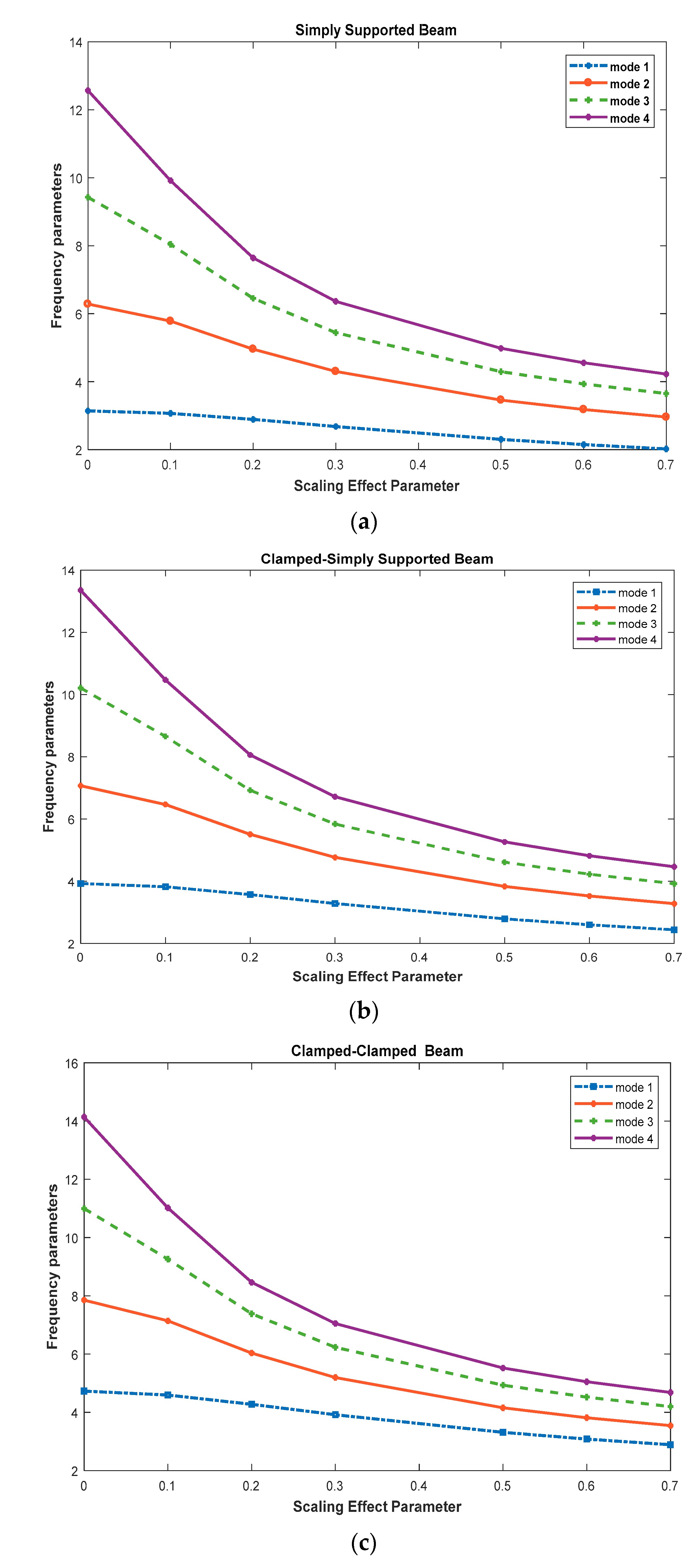
6. Numerical Results and Discussions

The frequency parameter $\lambda$ has been obtained by solving Equation (15) using the Matlab program developed by the authors.

In the numerical evaluation, we have taken single-walled carbon nanotube (SWNT) with the properties:

diameter $d=0.678\mathrm{nm}$; length $L=10\mathrm{d}$; Young’s Modulus $E=5.5\mathrm{TPa}$; $G=\frac{E}{\left[2\left(1+v\right)\right]}$; Poisson’s ratio $v=0.19$ and $I=\pi d^4/64$, α = 0.5 [11].

In

Table 1. Convergence of first three frequency parameters for Simply Supported beam.

N	First	Second	Third
3	2.302557	3.847474	5.058655
4	2.302557	3.466762	5.058655
5	2.302231	3.466762	4.323108
6	2.302231	3.460430	4.323108
7	2.302231	3.460430	4.294516
8	2.302231	3.460401	4.294516
9	2.302231	3.460401	4.294516
10	2.302231	3.460401	4.294516

we represent the convergence of first three frequency parameters for Simply Supported beam taking the Bernstein polynomials as shape function.

Further, the orthogonal Bernstein polynomials ${\widehat{\varphi }}_i$’ is defined in Equation (17), have been used to find frequency parameters. In

Table 2. Comparison of the convergence of first three frequency parameters for Simply Supported nanobeams using Bernstein polynomials and Orthogonal Bernstein polynomials.

Frequency Parameters	First		Second		Third
N	Orthogonal	Simple	Orthogonal	Simple	Orthogonal	Simple
3	2.3026	2.3026	3.8475	3.8474	5.0587	5.0586
4	2.3026	2.3026	3.4668	3.4668	5.0587	5.0586
5	2.3022	2.3022	3.4668	3.4668	4.3231	4.3231
6	2.3022	2.3022	3.4604	3.4604	4.3231	4.3231
7	2.3022	2.3022	3.4604	3.4604	4.2945	4.2945
8	2.3022	2.3022	3.4604	3.4604	4.2945	4.2945
9	2.3022	2.3022	3.4604	3.4604	4.2941	4.2941
10	2.3022	2.3022	3.4604	3.4604	4.2941	4.2941

, the convergence of first three frequency parameters for Simply Supported nanobeam is compared by using orthogonal Bernstein polynomials as well as Simple Bernstein polynomials with α = 0.5.

In

Table 3. Comparison of the convergence of Frequency Parameters with the results of Reference [18].

Frequency Parameters	First		Second		Third
N	Reference [18]	Present	[18]	Present	[18]	Present
3	2.3026	2.3026	3.8475	3.8474	5.0587	5.0586
4	2.3026	2.3026	3.4668	3.4668	5.0587	5.0586
5	2.3022	2.3022	3.4668	3.4668	4.3231	4.3231
6	2.3022	2.3022	3.4604	3.4604	4.3231	4.3231
7	2.3022	2.3022	3.4604	3.4604	4.2945	4.2945
8	2.3022	2.3022	3.4604	3.4604	4.2945	4.2945
9	2.3022	2.3022	3.4604	3.4604	4.2941	4.2941
10	2.3022	2.3022	3.4604	3.4604	4.2941	4.2941

we compare our numerical results with Behera and Chakraverty [18]. The results are found to be in good agreement. We observed that the number of approximations is same but the computational time is less while using orthogonal Bernstein polynomials. We observed that for N = 10 the run time is 6.743 s and for orthogonal Bernstein polynomial, it is 6.170 s by using Matlab programming.

Further, we have also used the Laguerre polynomials as shape functions and study the convergence of first three frequency parameters to have a comparison with Bernstein polynomials. In

Table 4. First three frequency parameters taking Laguerre polynomials as shape functions (S-S, α = 0.5).

N	First	Second	Third
3	2.3026	3.8475	5.0587
4	2.3026	3.4668	5.0587
5	2.3022	3.4668	4.3231
6	2.3022	3.4604	4.3231
7	2.3022	3.4604	4.2945
8	2.3022	3.4604	4.2945
9	2.3022	3.4604	4.2945
10	2.3022	3.4604	4.2941
11	2.3022	3.4604	4.2941

, we present the convergence of first three frequency parameters for Simply Supported nanobeam with scaling parameter α = 0.5 taking Laguerre polynomials as shape functions.

From Table 4, we may observe that we need at least 11 terms for the convergence of first three frequencies whereas in the case of orthogonal Bernstein polynomials, it starts converging from 10th term. It is worth mentioning that for getting the converged third frequency only, orthogonal Bernstein polynomials are a winner by one term in this particular case. So, in general, we may see that the number of terms for both the polynomials needs similar but as said earlier that orthogonal Bernstein polynomials have less computational complexity.

In

Table 5. Comparison of first three frequency parameters for Simply Supported nanobeam with different scaling parameters

Frequency Parameter		α = 0		α = 0.1	α = 0.3		α = 0.5		α = 0.7
OBPs	Reference [11]	OBPs	[11]	OBPs	[11]	OBPs	[11]	OBPs	[11]	OBPs
Simply Supported-Simply Supported (S-S)
First	3.1416	3.1416	3.0685	3.0685	2.6800	2.6800	2.3022	2.3022	2.0212	2.0212
Second	6.2832	6.2832	5.7817	5.7817	4.3013	4.3013	3.4604	3.4604	2.9585	2.9585
Third	9.4248	9.4248	8.0400	8.0400	5.4423	5.4423	4.2941	4.2941	3.6486	3.6486
Fourth	12.566	12.566	9.9162	9.9162	6.3630	6.3630	4.9820	4.9820	4.2234	4.2234
Clamped-Simply Supported (C-S)
First	3.9226	3.9226	3.8209	3.8209	3.2828	3.2828	2.7899	2.7899	2.4364	2.4364
Second	7.0686	7.0686	6.4649	6.4649	4.7668	4.7668	3.8325	3.8325	3.2776	3.2776
Third	10.210	10.210	8.6517	8.6517	5.8371	5.8371	4.6105	4.6105	3.9201	3.9201
Fourth	13.252	13.252	10.469	10.469	6.7145	6.7145	5.2633	5.2633	4.4645	4.4645
Clamped-Clamped (C-C)
First	4.7300	4.7300	4.5945	4.5945	3.9184	3.9184	3.3153	3.3153	2.8893	2.8893
Second	7.8532	7.8532	7.1402	7.1402	5.1963	5.1963	4.1561	4.1561	3.5462	3.5462
Third	10.996	10.996	9.2583	9.2583	6.2317	6.2317	4.9328	4.9328	4.1996	4.1996
Fourth	14.137	14.137	11.016	11.016	7.0482	7.0482	5.5213	5.5213	4.6817	4.6817

we compare first four frequency parameters with different scaling parameters and different boundary conditions with the result of Wang et al. [11]. The results are found to be in good agreement.

For nanobeams, the scaling effect parameter plays a significant influence. This may be visualized in Figure 1, where we represent the variation of first four frequency parameters with respect to scaling effect parameters for various boundary conditions, such as Figure 1a for Simply Supported-Simply Supported, Figure 1b for Clamped-Simply supported, and Figure 1c for Clamped-Clamped.

We observed that the frequency parameters are becoming smaller when the scaling effect parameters are increased. However, it is interesting to note that the deflection is high with respect to scaling effects for higher modes with various boundary conditions. Thus we may conclude that the nanobeams are more flexible due to small scale effects.

7. Conclusions

In this investigation, an efficient numerical technique has been developed for the study of vibration of Euler–Bernoulli nanobeam using Eringen’s nonlocal theory and considering the Bernstein polynomials as base functions. Bernstein polynomials are easy to handle different boundary conditions and also it takes less computational time. The convergence study of frequency parameters are studied in terms of tables. Furthermore, the results are in good agreement with Wang et al. [11]. Here we also introduce the Orthogonal Berstein Polynomials and we found that the number of approximations is same but the computational time is less while using orthogonal Bernstein polynomials. Further comparisons have also been made with other polynomials as shape functions viz. that of Laguerre polynomials. It is demonstrated that Laguerre polynomials take more terms with respect to particular frequency but the requirement of the number of terms compared to orthogonal Bernstein polynomials is not so significant. The main value of the use of the Bernstein polynomials takes less time in computation and simple computer implementation. A new convergence theorem has been developed here to show the theoretical convergence of displacement function with respect to the Bernstein polynomials.

Finally, we may conclude that this method may easily be extended to other nanostructures related vibration problems.

References

1. Peng, H.B.; Chang, C.W.; Aloni, S.; Yuzvinsky, T.D.; Zettl, A. Ultrahigh frequency nanotube resonators. Phys. Rev. Lett. 2006, 97, 087203. [Google Scholar] [CrossRef] [PubMed]
2. Dubey, A.; Sharma, G.; Mavroidis, C.; Tomassone, M.S.; Nikitczuk, K.; Yarmush, M.L. Computational studies of viral protein nano-actuators. J. Comput. Theor. Nanosci. 2004, 1, 18–28. [Google Scholar] [CrossRef]
3. Ruud, J.A.; Jervis, T.R.; Spaepan, F. Nanoindentation of Ag/Nimultilayered thin films. J. Appl. Phys. 1994, 75, 4969. [Google Scholar] [CrossRef]
4. Wang, L.F.; Hu, H.Y. Flexural wave propagation in single-walled carbon nanotubes. Phys. Rev. B 2005, 71, 195412. [Google Scholar] [CrossRef]
5. Eringen, A.C. Nonlocal polar elastic continua. Int. J. Eng. Sci. 1972, 10, 1–16. [Google Scholar] [CrossRef]
6. Reddy, J.N. Nonlocal theories for bending, buckling and vibration of beams. Int. J. Eng. Sci. 2007, 45, 288–307. [Google Scholar] [CrossRef]
7. Wang, C.M.; Kitipornchai, S.; Lim, C.W.; Eisenberger, M. Beambending solution based on nonlocal Timoshenko beam theory. J. Eng. Mech. ASCE 2008, 134, 475–481. [Google Scholar] [CrossRef]
8. Wang, Q. Wave propagation in carbon nanotubes via nonlocal continuum mechanics. J. Appl. Phys. 2005, 98, 124301. [Google Scholar] [CrossRef]
9. Zhang, Y.Q.; Liu, G.R.; Xie, X.Y. Free transverse vibrations of double-walled carbon nanotubes using a theory of nonlocal elasticity. Phys. Rev. B 2005, 71, 195404. [Google Scholar] [CrossRef]
10. Aydogdu, M. A general nonlocal beam theory: Its application to nanobeam bending, buckling and vibration. Low Dimens. Syst. Nanostruct. 2009, 41, 1651–1655. [Google Scholar] [CrossRef]
11. Wang, C.M.; Zhang, Y.Y.; He, X.Q. Vibration of nonlocal Timoshenko beams. Inst. Phys. 2007, 18, 105401. [Google Scholar] [CrossRef]
12. Phadikar, J.K.; Pradhan, S.C. Variational formulation and finite element analysis for nonlocal elastic nanobeams and nanoplates. Comput. Mater. Sci. 2010, 49, 492–499. [Google Scholar] [CrossRef]
13. Eltaher, M.A.; Emam, S.A.; Mahmoud, F.F. Free vibration analysis of functionally graded size-dependent nanobeams. Appl. Math. Comput. 2012, 218, 7406–7420. [Google Scholar] [CrossRef]
14. Mohammadi, B.; Ghannadpour, S.A.M. Energy approach vibration analysis of nonlocal Timoshenko beam theory. Procedia Eng. 2011, 10, 1766–1771. [Google Scholar] [CrossRef]
15. Roque, C.M.C.; Ferreira, A.J.M.; Reddy, J.N. Analysis of Timoshenko nanobeams with a nonlocal formulation and meshless method. Int. J. Eng. Sci. 2011, 49, 976–984. [Google Scholar] [CrossRef]
16. Pradhan, S.C.; Murmu, T. Application of nonlocal elasticity and DQM in the flapwise bending vibration of rotating nanocantilever. Physica E Low Dimens. Syst. Nanostruct. 2010, 42, 1944–1949. [Google Scholar] [CrossRef]
17. Jena, S.K.; Chakerverty, S. Free vibration analysis of Euler–Bernoulli Nanobeam using differential transform method. Int. J. Comput. Mater. Sci. Eng. 2018, 7, 1850020. [Google Scholar] [CrossRef]
18. Behera, L.; Chakraverty, S. Free vibration of Euler and Timoshenko nanobeams using boundary characteristic orthogonal polynomial. Appl. Nanosci. 2014, 4, 347–358. [Google Scholar] [CrossRef]
19. Singh, B.; Chakraverty, S. Use of characteristic orthogonal polynomials in two dimensions for transverse vibration of elliptic and circular plates with variable thickness. J. Sound Vib. 1994, 173, 289–299. [Google Scholar] [CrossRef]
20. Behera, L.; Chakraverty, S. Static analysis of nanobeams using the Rayleigh-Ritz method. J. Mech. Mater. Struct. 2017, 12, 603–616. [Google Scholar] [CrossRef]
21. Chakraverty, S.; Behera, L. Static and Dynamic Problems of Nanobeams and Nanoplates, 1st ed.; World Scientific Publishing Co.: Singapore, 2016. [Google Scholar]
22. Chakraverty, S. Vibration of Plates; CRC Press: Boca Raton, FL, USA, 2009. [Google Scholar]
23. Fernández-Sáez, J.; Zaera, R.; Loya, J.A.; Reddy, J.N. Bending of Euler-Bernoulli beams using Eringen’s integral formulation: A paradox resolved. Int. J. Eng. Sci. 2016, 99, 107–116. [Google Scholar] [CrossRef] [Green Version]
24. Joy, K.I. Bernstein Polynomials, On-Line Geometric Modeling Notes; Computer Science Department, University of California, Davis: Davis, CA, USA, 2000. [Google Scholar]
25. Civalek, O.; Akgoz, B. Free vibration analysis of microtubules as cytoskeleton components: Nonlocal Euler–Bernoulli beam modeling. Sci. Iran. Trans. B Mech. Eng. 2010, 17, 367–375. [Google Scholar]
Figure 1. Variation of frequency parameters (first four) with changes of scaling effects for different boundary conditions ((a) for Simply Supported (S-S), (b) for Clamped-Simply Supported (C-S), (c) for Clamped-Clamped (C-C)).
Jcs 03 00099 g001