Phase Change with Density Variation and Cylindrical Symmetry: Application to Selective Laser Melting

Abstract

In this paper we introduce an analytical approach for predicting the melting radius during powder melting in selective laser melting (SLM) with minimum computation duration. The purpose of this work is to evaluate the suggested analytical expression in determining the melt pool geometry for SLM processes, by considering heat transfer and phase change effects with density variation and cylindrical symmetry. This allows for rendering first findings of the melt pool numerical prediction during SLM using a quasi-real-time calculation, which will contribute significantly in the process design and control, especially when applying novel powders. We consider the heat transfer problem associated with a heat source of power $\dot{Q\prime } \left(\mathrm{W}/\mathrm{m}\right)$ per unit length, activated along the span of a semi-infinite fusible material. As soon as the line heat source is activated, melting commences along the line of the heat source and propagates cylindrically outwards. The temperature field is also cylindrically symmetric. At small times (i.e., neglecting gravity and Marangoni effects), when the density of the solid material is less than that of the molten material (i.e., in the case of metallic powders), an annulus is created of which the outer interface separates the molten material from the solid. In this work we include the effect of convection on the melting process, which is shown to be relatively important. We also justify that the assumption of constant but different properties between the two material phases (liquid and solid) does not introduce significant errors in the calculations. A more important result; however, is that, if we assume constant energy input per unit length, there is an optimum power of the heat source that would result to a maximum amount of molten material when the heat source is deactivated. The model described above can be suitably applied in the case of selective laser melting (SLM) when one considers the heat energy transferred to the metallic powder bed during scanning. Using a characteristic time and length for the process, we can model the energy transfer by the laser as a heat source per unit length. The model was applied in a set of five experimental data, and it was demonstrated that it has the potential to quantitatively describe the SLM process.

1. Introduction

Consider a semi-infinite solid slab, initially at temperature $T_{\infty }$. At time $t=0$, a continuous line heat source $\dot{Q\prime }\left(W/m\right)$ is activated along the line $r=0$. The temperature distribution in the semi-infinite medium is found to be [1] (pg. 261, Equation (5))

$$T=T_{\infty }+\frac{\dot{Q\prime }}{2 \pi k} E_1\left[\frac{r^2}{4 \alpha t}\right]$$

(1)

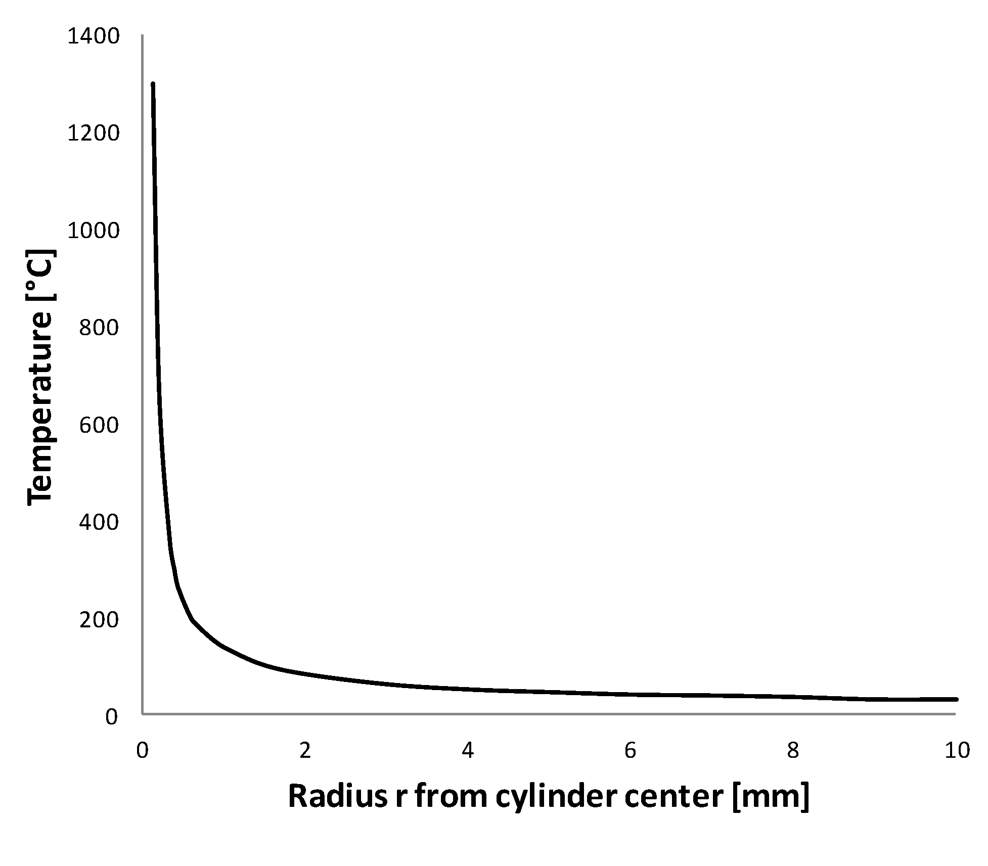
where $k$ is the thermal conductivity of the solid, and $E_1\left[x\right]$ is the exponential integral defined as $E_1\left[x\right]={{\displaystyle \int }}_x^{\infty }{e}^{-t}/t dt$. Similar to 1D Cartesian coordinates, there is no steady-state solution in 1D cylindrical coordinates. The temperature field is cylindrically symmetric, ranging from infinite at $r=0$ to $T_{\infty }$ at the far field. In reality though, if $T_{\infty }$ is less than the melting temperature $T_{\mathrm{melt}}$ of the material, the high temperature developed around $r=0$ would lead to melting of the material and a cylindrical interface would emerge separating the solid phase (metal powder) from the liquid phase (molten material). Hence, one has to take into consideration the different properties between the liquid and the solid phases and, in addition, the latent heat of melting L per unit mass at the interface. For a pure substance the interface is sharp at the melting temperature $T_{\mathrm{melt}}$ of the material, and it moves cylindrically outwards separating the two phases, solid and liquid. Similar arguments apply for the solidification process.

For the case of melting or solidification of a material due to a line source/sink, with constant but different properties between the liquid and solid phases but equal densities, an analytical solution has been obtained by Patterson [2], who combined two expressions similar to Equation (1). The boundary condition for the energy balance leads to an algebraic equation (characteristic equation) where the unknown, which can be considered to be an eigenvalue, is proportional to the position of the liquid-solid interface (i.e., the speed of melting of the material). The characteristic equation is monotonic with respect to the eigenvalue so there is only one single solution. The analysis is valid when the two phases have the same density. A review is given by Hu and Argyropoulos [3] and Alexiades and Solomon [4], where they present the major methods of mathematical modeling of solidification and melting. For the case where the two phases have different densities, the energy balance equation is different [4,5], and furthermore a convection term must be included in the heat equation of the liquid phase. The convection term can be obtained from the radially-symmetric continuity equation in cylindrical coordinates with constant density [4]. A similar approach is used for the analysis of melting of nanoparticles [6] and bubble growth and oscillations [7,8,9,10,11].

The major difference between bubble growth/oscillations and melting/solidification is that, for the former case, the bubble interface is set in motion by the pressure field, hence one has to solve the momentum equation. On the contrary, for the latter case the interface between the liquid and the solid phase is controlled by the conduction process; hence, the heat equation is decoupled from the momentum equation.

In this work, similar to Font et al. [6], we first solve the continuity equation in the liquid phase to find an expression for the velocity field using mass conservation. Subsequently we solve the heat equation in the two phases using a similarity transformation of the form $r/\sqrt{t}$, and through the energy boundary condition on the interface we obtain an algebraic (characteristic) equation for the eigenvalue $\lambda$, which is proportional to the location of the interface. Unlike Font et al. [6], we have neglected the kinetic energy term in the energy equation because it is small compared to other terms (see Section 2.2). Furthermore, if needed, an expression for the pressure field in the liquid phase can be obtained by substituting the expression of the velocity field in the radial momentum equation.

In this work, we apply the melting process described above, as a simplified model to describe the dynamics of selective laser melting (SLM) processes. Of course, for the prediction of the melt pool when a particular SLM or selective laser sintering (SLS) process is concerned, different mathematical approaches have been introduced and studied in the literature. Cheng and Chou [12] described an unsteady temperature simulation based on the finite element method (FEM) of the alloy IN718 [13], concentrating on the effect of varying scan length on the melt pool size. Polivnikova [14] studied the melt pool dynamics by means of a finite-element simulation for an SLS/SLM process. The numerical model considered the interaction between laser beam and powder material and phase transformations, while sub-models were developed to describe the capillary phenomena in the powder bed during SLS/SLM processing. Li et al. [15] investigated the heat transfer and phase transition during an SLM process with a moving volumetric heat source using the finite difference method. They proposed a model incorporating a phase function to differentiate the powder phase, melting liquid phase, dense solid phase and vaporized gas phase that also includes the volume shrinkage induced by the density change during the melting process. Letenneur et al. proposed a three dimensional analytical model which enables the calculation of the temperature distribution in powder for a Gaussian laser heat source [16]. In [17], Li et al. enhanced their proposed approach by including the residual stress field analysis. A similar numerical approach was presented by Tan et al. [18] based on a model addressing thermal, metallurgical, and mechanical effects for selective laser melting of titanium alloy. The aforementioned numerical models, although they consider all physical phenomena and elucidate the physical processes involved in the melt pool formation, are computationally intensive and cannot be used for real-time process control and optimization.

Thus, for the design of a thermal control system, the development of an efficient model is inevitable, and an analytical or semi-analytical model is necessary. On one hand, it should contain all the necessary physics, and on the other hand it should be characterized by the necessary computational efficiency, so that it can be used as an in-process reference for a control algorithm. Examples are available in the literature for pure heat transfer operations, such as scanned thermal processing [19,20] and for serial thermal processing methods such as arc welding [21] and SLM and laser cutting [22]. The model can be validated through an experimental apparatus via infrared camera and laser profilometry. This kind of sensor was used for output feedback in a closed loop geometry control system in a gas metal arc welding (GMAW) process [23]. Besides control, a simplified model can also be used to compute the structural shape and residual stresses [24]. In what follows, we develop a simple model based on the melting achieved due to a line heat source.

2. Mathematical Modeling

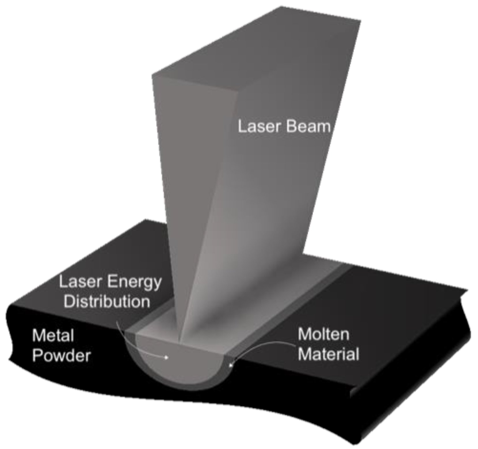
Our model is motivated by the melting achieved by a rapidly scanning laser beam moving along the span of a powder-bed [25]. Figure 1 and Figure 2 provide a detailed description of the model.

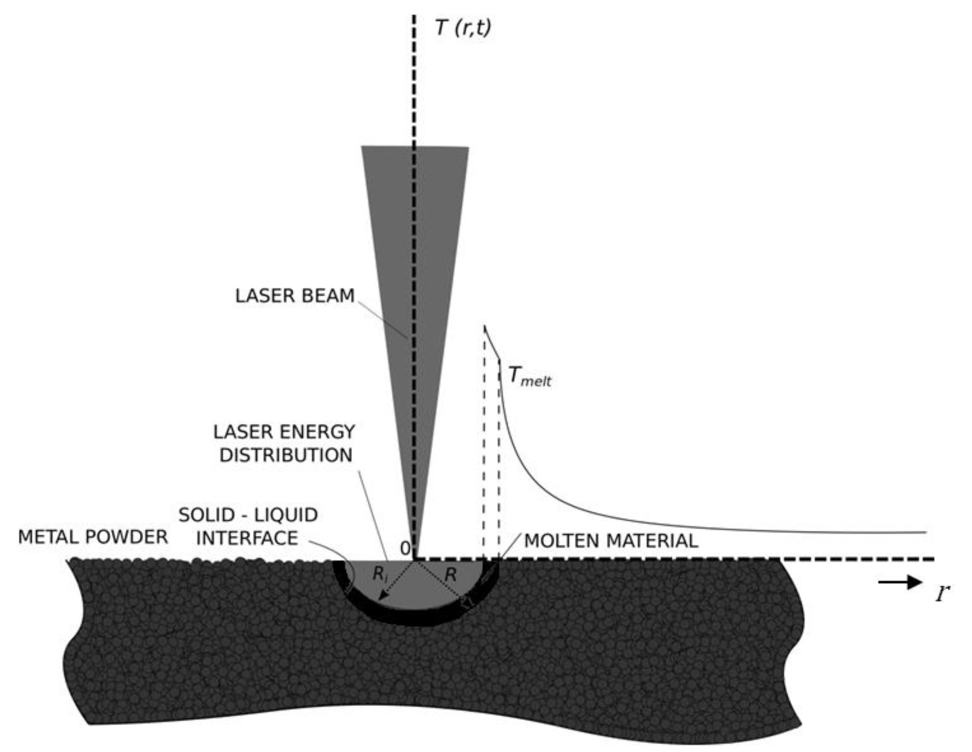
Initially, the semi-infinite bed of the fusible material (metal powder, powder-bed) is at the temperature $T_{\infty }$, lower than the melting temperature $T_{\mathrm{melt}}$ of the powder. A line heat source of strength $\dot{Q\prime }\left(W/m\right)$ is distributed initially along $r=0$ and is activated for a brief period of time $\tau$. The release of energy causes the temperature to increase higher than $T_{\mathrm{melt}}$, hence the melting commences at the origin. Because the density of the liquid phase is higher than the density of the solid phase (powder), an inner interface is created with radius $R_i$ (liquid-air interface, Figure 2). Hence, an annulus is created with an inner surface of radius $R_i\left[t\right]$, and an outer surface of radius $R\left[t\right]$. The latter separates the liquid (melted material) from the solid (powder) (i.e., $T\left[r=R\left[t\right]\right]=T_{\mathrm{melt}}$; Figure 2); assuming a pure substance, and by ignoring the kinetics of phase change in melting, the interface ($r=R\left[t\right]$) is sharp. Both the inner $r=R_i\left[t\right]$ and the outer $r=R\left[t\right]$ interfaces move in the positive r-direction with cylindrical symmetry, as shown in Figure 1 and Figure 2. During the time period $0<t\le \tau$, we assume that the laser beam is distributed evenly over the interface $R_i\left[t\right]$ due to irradiation and reflections of the laser beam, whereas at $t=0$ the laser beam is a line heat source distributed along $r=0$. For small times we can neglect gravity and Marangoni effects, hence the process is cylindrically symmetric, and, in addition, a radially-symmetric convection current $u_r\left[r,t\right]$ is developed in the annulus.

In order to apply this model to SLM of metallic powders a number of assumptions/parameters were adopted as described in detail in the following sections. The metal powder, which rests on a metal substrate, is molten by the scanning laser beam and solidifies into a metal deposit fused to the substrate. The density and thermal properties of the deposit are significantly different from the metal powder (see beginning of Section 3). We assume that during the initial stages of melting, the gravity and Marangoni effects can be neglected, hence the process is cylindrically symmetric. Furthermore, because the conductivity of the metal powder is on the order of 100 times smaller than that of the metal substrate, we assume that the heat transfer process is controlled by the powder bed, and the heat transfer process is prevalent in the molten pool [1]. Hence, during the initial melting of the powder, we neglect the presence of the metal substrate and assume a semi-infinite layer of metal powder.

The analysis that follows proceeds along the same lines as the analysis by Font et al. [6] for melting of a nanoparticle, and the analysis by Scriven [9] for bubble growth and oscillations [7,8,9,10,11], where an explicit expression for the convection term is obtained from the continuity equation and mass conservation.

2.1. Flow Field

Assuming constant density in the liquid phase (i.e., zero thermal expansion coefficient), the equation of continuity in cylindrical coordinates [26] takes the form $\frac{1}{r} \frac{\partial }{\partial r}\left({\rho }_{\ell } r u_{\mathrm{r}}\right)=0$. Integrating with respect to $r$, and enforcing the conditions at $r=R\left[t\right]$ or $r= R_i\left[t\right]$ we obtain:

$$u_{\mathrm{r}}\left[r,t\right]= \frac{ R\left[t\right] {\upsilon }_{\ell }}{r}= \frac{ R_i\left[t\right] {\dot{R}}_i\left[t\right]}{r}$$

(2)

where $u_{\mathrm{r}}\left[r,t\right]$ is the velocity of the fluid at radius r and time t and ${\upsilon }_{\ell } \equiv u_{\mathrm{r}}\left[r=R\left[t\right],t\right]$ is the velocity of the fluid perpendicular to the interface $r=R\left[t\right]$. Similar expressions are obtained in the case of a moving spherical interface [6,7,8,9,10,11]. We should point out that, while the velocity of the fluid (molten material) is ${\dot{R}}_i\left[t\right]$ at $r=R_i$, its velocity is not $\dot{R}\left[t\right]$ at $r=R\left[t\right]$. In order to find a relation for ${\upsilon }_{\ell }$ we use mass conservation in a frame moving with the interface to obtain

$$-{\rho }_s \dot{R}\left[t\right]=\left({\upsilon }_{\ell }-\dot{R}\left[t\right]\right) {\rho }_{\ell },$$

where ${\rho }_s$ is the density of the solid and ${\rho }_{\ell }$ is the density of the liquid at the melting temperature $T_{\mathrm{melt}}$, which can be is resolved to

$${\upsilon }_{\ell }=\frac{\left({\rho }_{\ell }-{\rho }_s\right)}{{\rho }_{\ell }} \dot{R}\left[t\right].$$

(3)

This is the equation obtained by Özişik [5] (pg. 403, Equation (10-9b)). To relate $R_i\left[t\right]$ to $R\left[t\right]$, we use mass conservation [6] on a unit span of the annulus of the molten pool to obtain

$$\frac{1}{2}\frac{\mathrm{d}}{\mathrm{d}t}\left[{\rho }_{\ell } \pi \left(R{\left[t\right]}^2-R_i{\left[t\right]}^2\right)\right]=\pi {\rho }_s R\left[t\right]\dot{R}\left[t\right].$$

Integrating above expression we obtain

$$\begin{gathered} {\rho }_{\ell } \left(R{\left[t\right]}^2-R_i{\left[t\right]}^2\right)={\rho }_s R{\left[t\right]}^2 \\ \Rightarrow R\left[t\right]\sqrt{\frac{{\rho }_{\ell }-{\rho }_s}{{\rho }_{\ell }}}=R_i\left[t\right] \end{gathered}$$

(4)

Substituting Equation (3) or Equation (4) in Equation (2), we obtain an equation for the velocity field in terms of the location $R\left[t\right]$ and velocity $\dot{R}\left[t\right]$ of the interface:

$$u_{\mathrm{r}}\left[r,t\right]= \frac{\left({\rho }_{\ell }-{\rho }_s\right)}{{\rho }_{\ell }} \frac{ R\left[t\right] \dot{R}\left[t\right]}{r}$$

(5)

2.2. Governing Equations

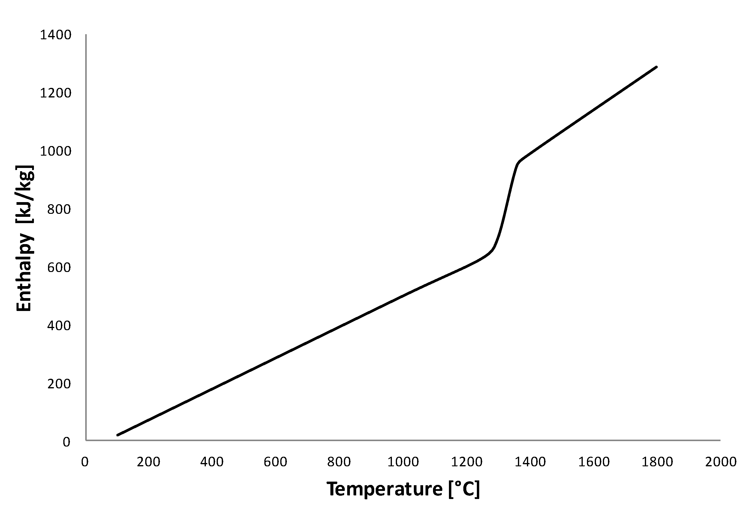
Assuming that the properties of the powder and the molten material are constant but different, the mathematical formulation of this problem is given by

$$\begin{gathered} {\rho }_{\ell } c_{p\ell } \left(\frac{\partial T_{\ell }}{\partial t} + u_{\mathrm{r}}\left[r,t\right]\frac{\partial T_{\ell }}{\partial r}\right)= \frac{1}{r} \frac{\partial }{\partial r}\left(k_{\ell } r \frac{\partial T_{\ell }}{\partial r}\right) \mathrm{in}\mathrm{the}\mathrm{region} R_i\left[t\right] <r <R\left[t\right],t>0 \\ {\rho }_s c_{ps} \frac{\partial T_s}{\partial t}= \frac{1}{r} \frac{\partial }{\partial r}\left(k_s r \frac{\partial T_s}{\partial r}\right) \mathrm{in}\mathrm{the}\mathrm{region} R\left[t\right] <r <\infty ,t>0 \end{gathered}$$

(6)

where, as mentioned earlier (Equation (5)),

$$u_{\mathrm{r}}\left[r,t\right]= \frac{\left({\rho }_{\ell }-{\rho }_s\right)}{{\rho }_{\ell }} \frac{ R\left[t\right] \dot{R}\left[t\right]}{r}$$

with the initial condition

$$T=T_{\infty } \mathrm{at}t=0$$

and the boundary conditions

$$\begin{gathered} -\pi r k_{\ell } \frac{\partial T_{\ell }}{\partial r}={\dot{Q}}^{\prime }\mathrm{at} r=R_i\left[t\right],t>0, \\ {T}_s= T_{\ell }= T_{\mathrm{melt}} \mathrm{at}r=R\left[t\right], t>0, \\ {k}_s \frac{\partial T_s}{\partial r}- k_{\ell } \frac{\partial T_{\ell }}{\partial r}=L {\rho }_s \frac{dR}{dt} \mathrm{at}r=R\left[t\right],t>0 \\ {T}_s\to T_{\infty } \mathrm{as}r\to \infty ,t>0. \end{gathered}$$

(7)

In the above equations, $\rho$ represents the density, $c_p$ the specific heat, and $k$ the conductivity, while the subscripts $\ell$ and $s$ represent the liquid and the solid phases, respectively. As shown in Özişik [5] (pg. 403, Equation (10-10a)), the third boundary condition is developed by performing an energy balance across the melting interface at $r=R\left[t\right]$. In a coordinate system moving with the interface the energy balance takes the form:

$$\dot{R}\left[t\right] H_s {\rho }_s+k_s\frac{\partial T_s}{\partial r}= \left(\left(\dot{R}\left[t\right]-{\upsilon }_{\ell }\right)H_{\ell }{\rho }_{\ell }+ k_{\ell }\frac{\partial T_{\ell }}{\partial r}\right)$$

If we substitute Equation (3) for ${\upsilon }_{\ell }$ we obtain

$$k_s\frac{\partial T_s}{\partial r}-k_{\ell }\frac{\partial T_{\ell }}{\partial r}= \dot{R}\left[t\right] \left(H_{\ell } {\rho }_{\ell }-\frac{\left({\rho }_{\ell }-{\rho }_s\right)}{{\rho }_{\ell }}{H}_{\ell } {\rho }_{\ell }-H_s {\rho }_s\right)$$

$$\Rightarrow k_s\frac{\partial T_s}{\partial r}-k_{\ell }\frac{\partial T_{\ell }}{\partial r}= \dot{R}\left[t\right] \left(H_{\ell } {\rho }_{\ell }-\left({\rho }_{\ell }-{\rho }_s\right) H_{\ell }-H_s {\rho }_s\right)$$

which is finally simplified to

$$\Rightarrow k_s\frac{\partial T_s}{\partial r}-k_{\ell }\frac{\partial T_{\ell }}{\partial r}= \dot{R}\left[t\right] {\rho }_s \left(H_{\ell }-H_s\right)=\dot{R}\left[t\right] {\rho }_s L,$$

where $L$ is the latent heat, $L=H_{\ell }-H_s$.

A common mistake that appears in phase change problems with density variations is the exclusion of the kinetic energy term [4,6]. This term is the consequence of the density change which forces the fluid to move, and results in a kinetic energy deficit or surplus. This term is equal to $\pm \frac{{\rho }_s}{2} {\left(1-\frac{{\rho }_s}{{\rho }_{\ell }}\right)}^2{\left(\dot{R}\left[t\right]\right)}^3$ and it is usually excluded if it is small compared to the term related to the latent heat $\left(\dot{R}\left[t\right] {\rho }_s L\right)$. It is important only at very small times and when the value of the latent heat $L$ is small [4]; an exception is the melting of nanoparticles [6]. In our simulation the latent heat is of the order $L\sim {10}^5$ (J/kg) and the smaller value of the activation time $\tau \sim$0.0001 (s). As we will show later $\dot{R}\left[t\right]=\frac{\lambda \sqrt{{\alpha }_{\ell } }}{\sqrt{t}}$, hence the kinetic energy term is of the order $\sim {10}^{-2}$ (kg/s³) and it does not introduce any significant error. The important advantage of neglecting this term is that it allows for a similarity solution for the system of equations [2,4,5] in the form $z=r/R\left[t\right]$. The partial derivatives transform as follows:

$$\frac{\partial }{\partial r}= \frac{1}{R\left[t\right]} \frac{\partial }{\partial z},\frac{\partial }{\partial t}=\frac{\partial }{\partial t}- \frac{r \dot{R}\left[t\right] }{R{\left[t\right]}^2} \frac{\partial }{\partial z}.$$

Substituting in the partial differential Equations (6) and the boundary conditions (7), we obtain the following system of ordinary differential equations, which we assume that they are independent of time ($t$):

$${\rho }_{\ell }{c}_{p\ell } \left( - \frac{r \dot{R}\left[t\right] }{R{\left[t\right]}^2} \frac{\mathrm{d}{T}_{\ell }}{\mathrm{d}z}+ \frac{u_{\mathrm{r}}\left[r,t\right]}{R\left[t\right]}\frac{\mathrm{d}{T}_{\ell }}{\mathrm{d}z}\right)= \frac{1}{r R\left[t\right]} \frac{\mathrm{d}}{\mathrm{d}z}\left(k_{\ell } \frac{r}{R\left[t\right]} \frac{\mathrm{d}{T}_{\ell }}{\mathrm{d}z}\right) \mathrm{for}\frac{R_i\left[t\right]}{R\left[t\right]} <z <1$$

$${\rho }_s c_{ps}\left( - \frac{r \dot{R}\left[t\right] }{R{\left[t\right]}^2} \frac{\mathrm{d}{T}_s}{\mathrm{d}z}\right)= \frac{1}{r R\left[t\right]} \frac{\mathrm{d}}{\mathrm{d}z}\left(k_s \frac{r}{R\left[t\right]} \frac{\mathrm{d}{T}_s}{\mathrm{d}z}\right) \mathrm{for} 1<z <\infty$$

with boundary conditions

$$-\pi \frac{r}{R\left[t\right]} k_{\ell } \frac{\mathrm{d}{T}_{\ell }}{\mathrm{d}z}=\dot{Q^{\prime }} \mathrm{at}z=\frac{R_i\left[t\right]}{R\left[t\right]},$$

$$T_s= T_{\ell }= T_{\mathrm{melt}} \mathrm{at}z=1$$

$$\frac{k_s}{R\left[t\right]} \frac{\mathrm{d}{T}_s}{\mathrm{dz}}- \frac{k_{\ell }}{R\left[t\right]} \frac{\mathrm{d}{T}_{\ell }}{\mathrm{d}z}=L {\rho }_s \frac{dR}{dt} \mathrm{at}r=1,$$

$$T_s\to T_{\infty } \mathrm{at}z\to \infty .$$

Note that the last equation also describes the initial condition. Multiplying by $R{\left[t\right]}^2$ and substituting the expression for $u_{\mathrm{r}}\left[r,t\right]= \frac{\left({\rho }_{\ell }-{\rho }_s\right)}{{\rho }_{\ell }} \frac{ R\left[t\right] \dot{R}\left[t\right]}{r}$ (Equation (4)) and $R_i\left[t\right]=R\left[t\right]\sqrt{\frac{{\rho }_{\ell }-{\rho }_s}{{\rho }_{\ell }}}$ (Equation (4)), the above system simplifies to

$${\rho }_{\ell }{c}_{p\ell } \left( - \frac{r R\left[t\right] \dot{R}\left[t\right] }{R\left[t\right]} \frac{\mathrm{d}{T}_{\ell }}{\mathrm{d}z}+ \frac{R{\left[t\right]}^2\left({\rho }_{\ell }-{\rho }_s\right)}{{\rho }_{\ell }} \frac{\dot{R}\left[t\right]}{r}\frac{\mathrm{d}{T}_{\ell }}{\mathrm{d}z}\right)= \frac{R\left[t\right]}{r } \frac{\mathrm{d}}{\mathrm{d}z}\left(k_{\ell } \frac{r}{R\left[t\right]} \frac{\mathrm{d}{T}_{\ell }}{\mathrm{d}z}\right) \mathrm{for}\sqrt{\frac{{\rho }_{\ell }-{\rho }_s}{{\rho }_{\ell }}} <z <1$$

$${\rho }_s c_{ps}\left( - \frac{r R\left[t\right] \dot{R}\left[t\right] }{R\left[t\right]} \frac{\mathrm{d}{T}_s}{\mathrm{d}z}\right)= \frac{R\left[t\right]}{r} \frac{\mathrm{d}}{\mathrm{d}z}\left(k_s \frac{r}{R\left[t\right]} \frac{\mathrm{d}{T}_s}{\mathrm{d}z}\right) \mathrm{for} 1 <z <\infty$$

with boundary conditions

$$-\pi z k_{\ell } \frac{\mathrm{d}{T}_{\ell }}{\mathrm{d}z}=\dot{Q^{\prime }} \mathrm{at}z=\sqrt{\frac{{\rho }_{\ell }-{\rho }_s}{{\rho }_{\ell }}},$$

$$T_s= T_{\ell }= T_{\mathrm{melt}} \mathrm{at}z=1,$$

$$k_s \frac{\mathrm{d}{T}_s}{\mathrm{dz}}- k_{\ell } \frac{\mathrm{d}{T}_{\ell }}{\mathrm{d}z}=L {\rho }_s R\left[t\right]\frac{dR}{dt} \mathrm{at}z=1,$$

$$T_s\to T_{\infty } \mathrm{as}z\to \infty .$$

Above equations are independent of time only if $R\left[t\right]\dot{R}\left[t\right]=c$ (i.e., $R\left[t\right]=\sqrt{2 c t}$, where $c$ is a constant to be determined). We finally obtain:

$${\rho }_{\ell } c_{p\ell } \left( - z c \frac{\mathrm{d}{T}_{\ell }}{\mathrm{d}z}+ \frac{\left({\rho }_{\ell }-{\rho }_s\right)}{{\rho }_{\ell }} \frac{c}{z}\frac{\mathrm{d}{T}_{\ell }}{\mathrm{d}z}\right)= \frac{1}{z } \frac{\mathrm{d}}{\mathrm{d}z}\left(k_{\ell } z \frac{\mathrm{d}{T}_{\ell }}{\mathrm{d}z}\right) \mathrm{for}\sqrt{\frac{{\rho }_{\ell }-{\rho }_s}{{\rho }_{\ell }}} <z <1$$

$${\rho }_{s }{c}_{ps}\left( - z c \frac{\mathrm{d}{T}_s}{\mathrm{d}z}\right)= \frac{1}{z} \frac{\mathrm{d}}{\mathrm{d}z}\left(k_s\left[T\right] z \frac{\mathrm{d}{T}_s}{\mathrm{d}z}\right) \mathrm{for} 1<z <\infty$$

with boundary conditions

$$-\pi z k_{\ell }\left[T\right] \frac{\mathrm{d}{T}_{\ell }}{\mathrm{d}z}=\dot{Q^{\prime }} \mathrm{at}z=\sqrt{\frac{{\rho }_{\ell }-{\rho }_s}{{\rho }_{\ell }}},$$

$$T_s= T_{\ell }= T_{\mathrm{melt}} \mathrm{at}z=1$$

$$k_s\left[T\right] \frac{\mathrm{d}{T}_s}{\mathrm{dz}}- k_{\ell }\left[T\right] \frac{\mathrm{d}{T}_{\ell }}{\mathrm{d}z}=L {\rho }_s\left[{\rm T}\right] c \mathrm{at}z=1,$$

$$T_s\to T_{\infty } \mathrm{as}z\to \infty ,$$

where the square brackets [T] indicate a temperature dependency of the thermal conductivity k and the density ρ. The above system can be brought in the following form:

$$\begin{gathered} \frac{{\mathrm{d}}^2{T}_{\ell }}{\mathrm{d}{z}^2}+\left(\frac{1}{z}+ \frac{z c}{{\alpha }_{\ell }} - \frac{\epsilon }{{\alpha }_{\ell }} \frac{c}{z}\right)\frac{\mathrm{d}{T}_{\ell }}{\mathrm{d}z}=0 \mathrm{for}\sqrt{\epsilon } <z <1 \\ \frac{{\mathrm{d}}^2{T}_s}{\mathrm{d}{z}^2}+ \left(\frac{1}{z} + \frac{z c}{{\alpha }_s}\right)\frac{\mathrm{d}{T}_s}{\mathrm{d}z} =0 \mathrm{for}1 <z <\infty \end{gathered}$$

(8)

with boundary conditions

$$\begin{gathered} -\pi z k_{\ell } \frac{\mathrm{d}{T}_{\ell }}{\mathrm{d}z}=\dot{Q^{\prime }} \mathrm{at} z=\sqrt{\epsilon }, \\ {T}_s= T_{\ell }= T_{\mathrm{melt}} \mathrm{at}z=1, \\ {k}_s \frac{\mathrm{d}{T}_s}{\mathrm{dz}}- k_{\ell } \frac{\mathrm{d}{T}_{\ell }}{\mathrm{d}z}=L {\rho }_s c \mathrm{at}z=1, \\ {T}_s\to T_{\infty } \mathrm{as}z\to \infty . \end{gathered}$$

(9)

where $\alpha = k/\left(\rho c_p\right)$ is the thermal diffusivity and $\epsilon =\left({\rho }_{\ell }-{\rho }_s\right)/ {\rho }_{\ell }$. Note that if we set $\epsilon =0$, the effect of convection is “switched off”; however, the density difference is still included in the energy balance equation (Equation (9), third equation; i.e., we obtain a result similar to Özişik [5] (pg. 415).

2.3. Characteristic Equation

The system of ordinary differential equations (ODEs) (8) can be integrated once to obtain

$$\begin{gathered} \frac{\mathrm{d}{T}_{\ell }}{\mathrm{d}z}= A_1{e}^{-c{z}^2/\left(2{\alpha }_{\ell }\right)} z^{\left(c\epsilon /{\alpha }_{\ell }-1\right)}, \\ \frac{\mathrm{d}{T}_s}{\mathrm{d}z}=A_2{e}^{-c{z}^2/\left(2{\alpha }_s\right)} z^{-1}. \end{gathered}$$

(10)

Using the first boundary condition from Equations (9) we obtain that

$$A_1= -\frac{\dot{Q\prime } e^{\frac{c\epsilon }{2{\alpha }_{\ell }}} {\epsilon }^{-\frac{c\epsilon }{2{\alpha }_{\ell }}}}{\pi k_{\ell }}=-\frac{\dot{Q\prime } }{\pi k_{\ell }} {\left(\frac{e}{\epsilon }\right)}^{\frac{c\epsilon }{2{\alpha }_{\ell }}}.$$

(11)

An expression for $T_{\ell }$ can be obtained in the form of the incomplete gamma function and the second boundary condition (Equation (9)); however, it is not required in order to obtain an expression for the eigenvalue $c$. An expression for $T_s$ can be obtained in the form of the exponential integral $E_1\left[x\right]={{\displaystyle \int }}_x^{\infty }{e}^{-t}/t \mathrm{d}t$ using the substitution $\zeta =c{z}^2/\left(2{\alpha }_s\right)$:

$$\frac{\mathrm{d}{T}_s}{\mathrm{d}\zeta }=\frac{A_2}{2}{e}^{-\zeta }/ \zeta .$$

Employing the second and fourth boundary conditions we can obtain an expression for $A_2$:

$$A_2=\frac{2\left(T_{\infty }-T_{\mathrm{melt}}\right)}{E_1\left[c/\left(2{\alpha }_s\right)\right]}$$

(12)

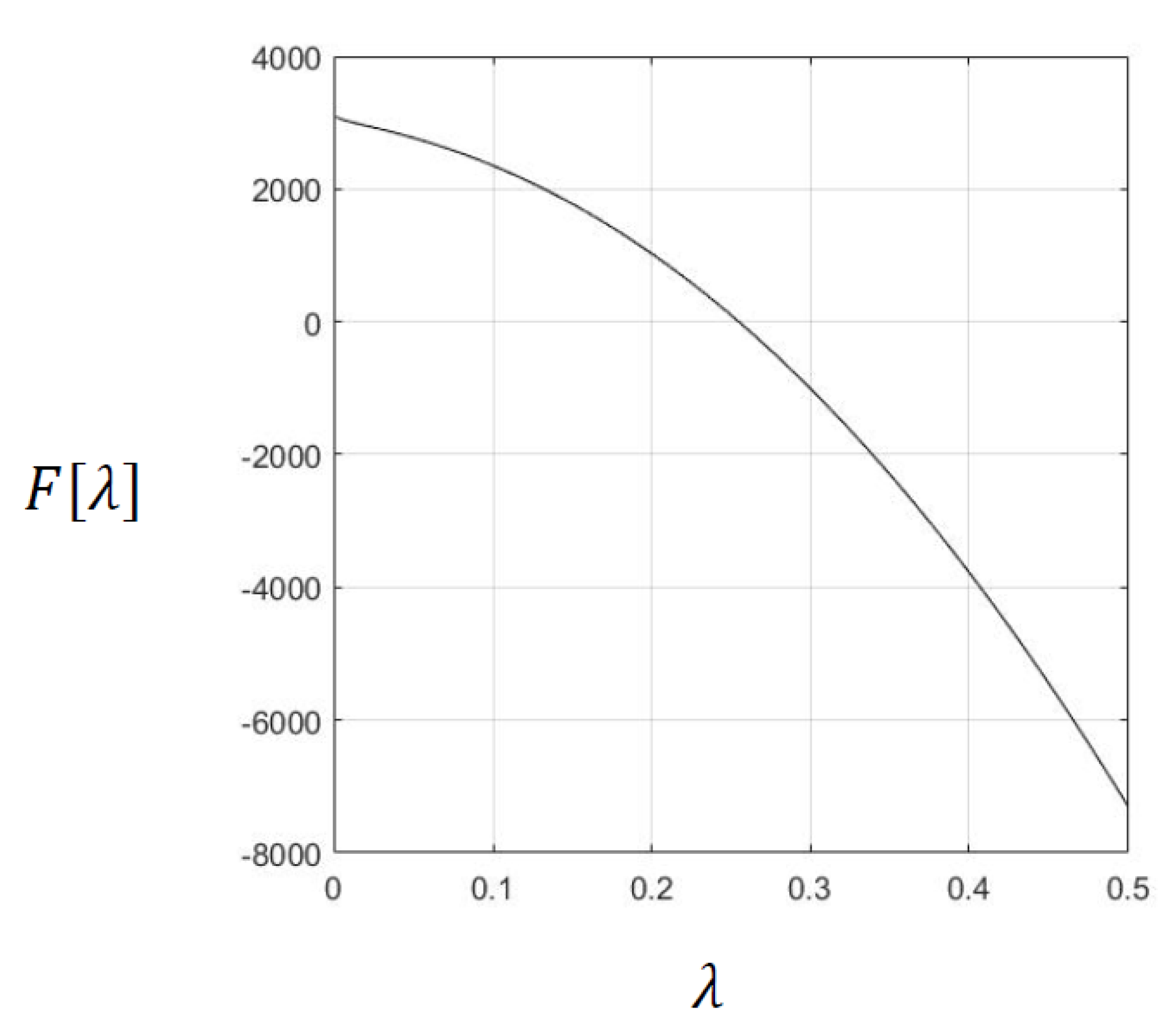
Substituting (10)–(12) in the third boundary condition of Equation (9), we obtain an algebraic equation (i.e., the characteristic equation) for $c$:

$$\frac{\dot{Q\prime } }{\pi } {\left(\frac{e}{\epsilon }\right)}^{c\epsilon /\left(2{\alpha }_{\ell }\right)}{e}^{-c/\left(2{\alpha }_{\ell }\right)}+ k_s \frac{2\left(T_{\infty }-T_{\mathrm{melt}}\right)}{E_1\left[c/\left(2{\alpha }_s\right)\right]}{e}^{-c/\left(2{\alpha }_s\right)}=L {\rho }_s c$$

If we replace $c$ with $c=2 {\alpha }_{\ell } {\lambda }^2$, we obtain a result similar to Carslaw and Jaeger [26] (pg. 296):

$$\begin{gathered} R\left[t\right]=2 \lambda \sqrt{{\alpha }_{\ell } t}, \\ F\left[\lambda \right]= \frac{\dot{Q\prime } }{\pi }{e}^{-{\lambda }^2}{\left(\frac{e}{\epsilon }\right)}^{\left({\lambda }^2\epsilon \right)}+\frac{2 k_s \left(T_{\infty }-T_{\mathrm{melt}}\right)e^{\left(-{\lambda }^2{\alpha }_{\ell }/{\alpha }_s\right)}}{E_1\left[{\lambda }^2 {\alpha }_{\ell }/{\alpha }_s\right]}-2 L {\rho }_s {\lambda }^2 {\alpha }_{\ell }=0. \end{gathered}$$

(13)

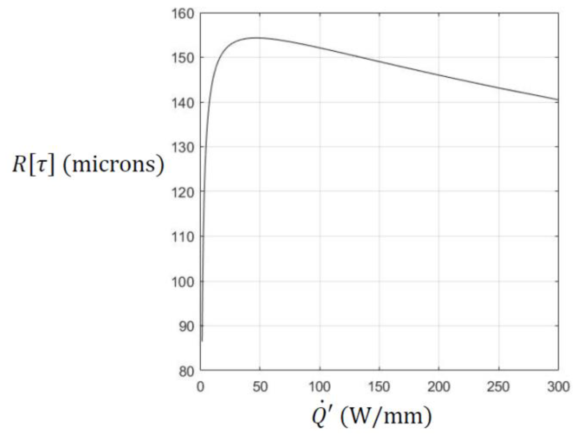
The factor 1/2, instead of 1/4, is due to the fact that we have considered a semi-infinite domain instead of an infinite domain. We can reproduce the result by Carslaw and Jaeger [1] if we neglect the convection term (i.e., if we set $\epsilon =0$, and replace $E_1\left[x\right]$ with $E_1\left[x\right]=-Ei\left[-x\right])$. If we know the properties of the material and the power $\dot{Q\prime }$ per unit length of the heat source, the above equation can be solved to find $\lambda$; hence the location of the liquid-solid interface $R\left[t\right]$ can be obtained for the time period $\tau$ that the heat source is activated.

3. Numerical Results of the Characteristic Equation

3.1. Application for Material Properties of IN718 Powder

The final result of the previous section was the transcendental equation (characteristic Equation (13)) for the constant $\lambda$, through which we obtained the velocity of the interface (i.e., the speed of melting of the material). Equation (13) is monotonic so there is only one single value for the eigenvalue $\lambda$ that satisfies the equation [2,5]. Furthermore, the effect of convection was to enhance the effect of the power $\dot{Q\prime }$, because the term ${\left(e/\epsilon \right)}^{\left({\lambda }^2\epsilon \right)}$ is always greater than one. Hence, we expect that the effect of convection would lead to larger values of $\lambda$ and, consequently, of the radius $R\left[t\right]$ of the melted material. The thermophysical properties of solid and liquid IN718 alloy were taken from the literature [12,13,27]. For our calculations we used the following values for the properties of the material which resembled the average IN718 powder properties for temperature close to melting point (i.e., in the range 800–1000 °C:

$${\rho }_{\ell }=7756 \mathrm{kg}/{\mathrm{m}}^3, c_{p\ell }=643 \mathrm{J}/\left(\mathrm{kg}·\mathrm{K}\right),k_{\ell }=26.63\mathrm{W}/\left(\mathrm{m}·\mathrm{K}\right),$$

$${\rho }_s=3926 \mathrm{kg}/{\mathrm{m}}^3, c_{ps}=351 \mathrm{J}/\left(\mathrm{kg}·\mathrm{K}\right),k_s=0.37\mathrm{W}/\left(\mathrm{m}·\mathrm{K}\right),$$

$$\begin{gathered} T_{\mathrm{melt}}=1300 °\mathrm{C},T_{\infty }=20 °\mathrm{C},L=\left(643-351\right)\times \left(1300+273.15\right) \mathrm{J}/\mathrm{kg}=459360\mathrm{J}/\mathrm{kg}, \\ \epsilon =0.4934. \end{gathered}$$

The melting temperature $T_{\mathrm{melt}}=$1300 °C used to model the melt pool was averaged from the liquid-solid phase distribution ranging from 1260 to 1336 °C [27]. An experimental measurement of enthalpy as a function of temperature indicating the temperature range for the liquid-solid phase change is shown in Figure 3 [28].

As an example, we set the power $\dot{Q\prime }=10000 \mathrm{W}/\mathrm{m}$. In Figure 4, we show a plot of the function $F\left[\lambda \right]$ vs $\lambda$. As mentioned earlier, the function $F\left[\lambda \right]$ is monotonic and it is straightforward to obtain numerically the root $\lambda =0.255$, hence the radius of the interface is $R\left[t\right]=2 \lambda \sqrt{{\alpha }_{\ell } t}=0.0012 \sqrt{t} \mathrm{m}$. This expression is valid while the heat source is activated (i.e., $0 \le t\le \tau )$.

To evaluate the effect of convection we set the parameter of the density ratio $\epsilon$ equal to zero. As expected the eigenvalue $\lambda$ decreased to $\lambda =0.2471$. The decrease in radius was of the order of 3%, hence the effect of convection is relatively important.

Equation (13) was derived based on the fact that the properties of both the liquid and solid phase are constant. In order to evaluate the effect of this assumption, we increased the properties of the liquid phase by 10%. The new root is $\lambda =0.2545$, which is 0.1% lower from the original root $\lambda =0.2549$, hence we can claim that our assumption of constant properties has limited impact on the results.

The temperature distribution in the solid powder as a function of the radius r from the cylinder center starting at the liquid-solid interface (i.e., radius of the molten pool of 0.12 mm), as calculated by solving Equation (10), is shown in Figure 5.

3.2. Optimum Value of the Line Heat Source

While the heat source is active (for the time period $\tau$), the location of the interface of the melted material is given by $R\left[t\right]=2 \lambda \sqrt{{\alpha }_{\ell } t}$ for $t\le \tau$. Of course, melting may continue for a brief period of time after the heat source is deactivated; however, this is beyond the scope of the current work. As expected, the longer the time period $\tau$ and the higher the power $\dot{Q\prime }$, the larger the radius $R\left[\tau \right]$. This raises the question on how the power is affecting the radius of melting for a fixed value of energy input per unit length:

$$Q\prime =\dot{Q\prime }·\tau (\mathrm{J}/\mathrm{m}).$$

(14)

Hence, in Equation (13), we replaced $\dot{Q\prime }$ with $Q\prime /\tau$, and found the value of the eigenvalue $\lambda$ as a function of the activation time $\tau$ of the heat source. For each value of the eigenvalue we determined the radius of the melted material at time $\tau$ (i.e., $R\left[\tau \right]=2 \lambda \sqrt{{\alpha }_{\ell } \tau })$. As an example, we set the total energy input to $Q\prime =150(\mathrm{J}/\mathrm{m}$). For the range of $\tau$ between 0.0001 and 0.1, we obtained that there was an optimum power per unit length $\dot{Q\prime },$ such that $R\left[\tau \right]$ was maximized, as shown in Figure 6.

From the numerical solution of Equation (13) for a fixed amount of energy per length $Q\prime =150\mathrm{J}/\mathrm{m}$, we obtained that the optimum power of the line heat source was approximately $\dot{Q\prime }=48.4\mathrm{kW}/\mathrm{m}$, which would lead to a radius $R\left[\tau =0.0031s\right]=154 \mathrm{microns}$.

However, in real SLM processes such short time periods τ (i.e., velocities in the order of 100 m/s) are not feasible. State-of-the-art processing speeds were found in the literature to be in the order of 0.01 to 2 m/s for high performance metallic alloys with a laser power of 100 to 1000 W.

4. Application of the Model to an SLM Process

Selective laser melting (SLM) is an additive rapid manufacturing technique where a laser is used to fuse metal powder that consists of micro- and nano-particles, into a specified three-dimensional geometry. In this section, we will apply the results of Section 2 (Equation (13)) to experimental data obtained in an SLM (selective laser melting) manufacturing process.

In

Table 1. SLM experiments using the alloy IN718. In the table we show the data of the five experiments, the energy per unit length delivered by the laser, and the upper bound (i.e., the maximum possible radius of molten material).

	Experiment 1	Experiment 2	Experiment 3	Experiment 4	Experiment 5
$\dot{Q}$ (W)	$300$	$360$	$240$	$300$	300
$v$ (m/s)	1.6	1.6	1.6	1.92	1.28
width (μm)	147	139	110	127	140
depth (μm)	94	83	53	84	139
$Q\prime \left(\mathrm{J}/\mathrm{m}\right)$	188	225	150	156	234
Equivalent radius $R$ = $\sqrt{\mathrm{width}/2\times \mathrm{depth}}$	83	76	54	73	99
Maximum radius (Equation (15))	183	200	164	167	205
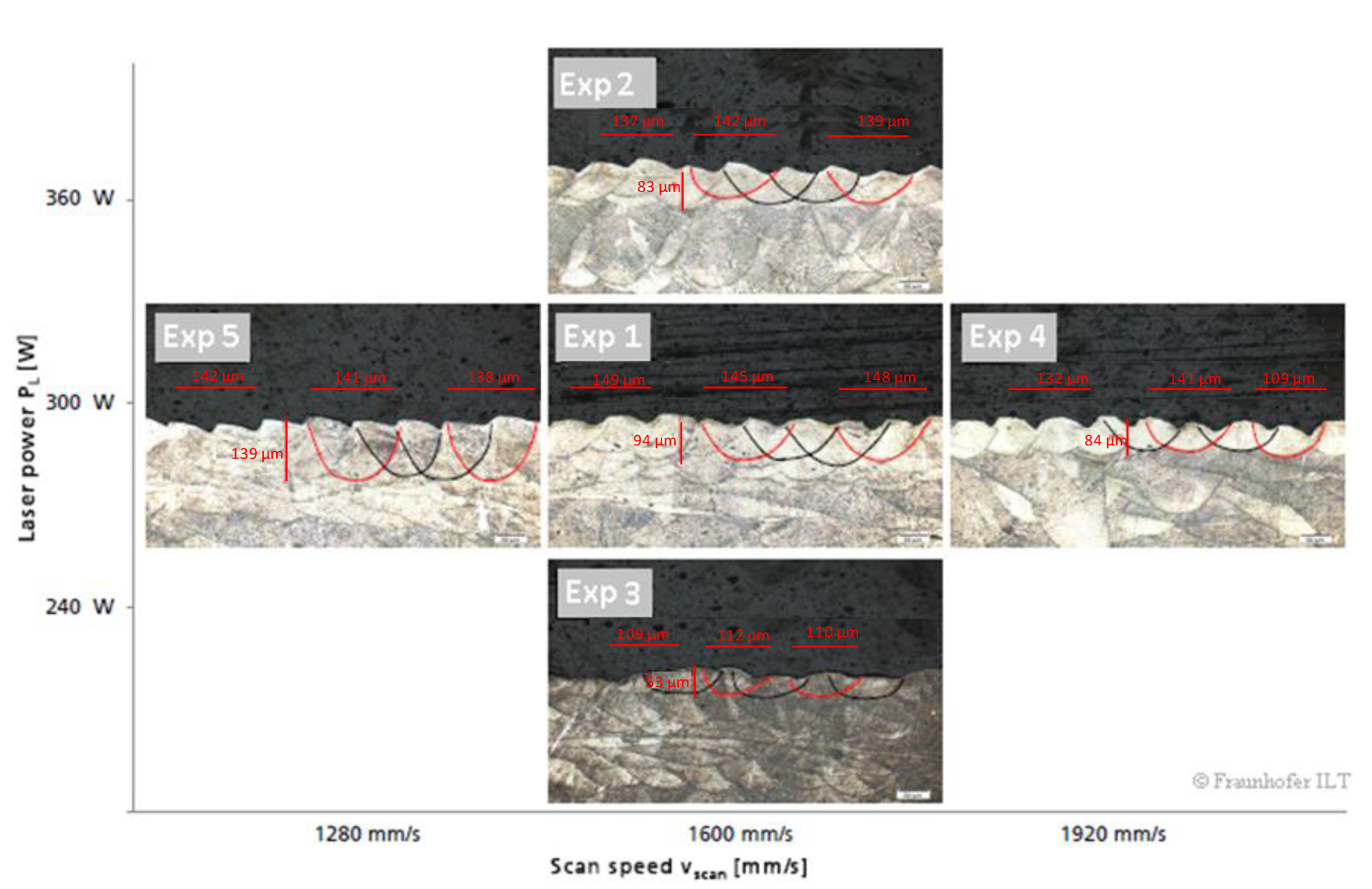
Relative error (%)	55	62	67	56	52

and

Table 2. SLM experiments using the alloy IN718. In the table we show the data of the five experiments, the equivalent heat source, the equivalent radius of the elliptical pool, and the radius calculated using Equation (13).

	Experiment 1	Experiment 2	Experiment 3	Experiment 4	Experiment 5
$\dot{Q}$ (W)	$300$	$360$	$240$	$300$	300
$v$ (m/s)	1.6	1.6	1.6	1.92	1.28
width (μm)	147	139	110	127	140
depth (μm)	94	83	53	84	139
$Q\prime \left(\mathrm{J}/\mathrm{m}\right)$	188	225	150	156	234
${\dot{Q}}_{eq}^{\prime }\left(\mathrm{W}/\mathrm{m}\right)$	1293	1552	1035	1078	1616
Equivalent radius R = $\sqrt{\mathrm{width}/2\times \mathrm{depth}}$	83	76	54	73	99
Numerical radius (Equation (13))	70	85	54	52	99
Relative error	15%	12%	<1%	28%	<1%

, we show the results of five experiments for the investigated IN718 alloy, based on the macrographs of a real SLM process, which are shown in Figure 7. The experiments were performed in the context of the MERLIN project on an SLM 280 HL machine (SLM solutions) with varying scan speed and laser powder [13]. Further process parameters were kept constant: laser focus diameter d_f = 90 μm (Gauss), hatch distance Δy = 80 μm, and layer thickness D = 30 μm. The weld pool geometry that resulted in each experiment approximates a cylindrical shape with a varying degree of deviation to the cylindrical shape because of surface (radiation, gas convection, Marangoni effect) and depth effects (conduction to solid substrate, gravity etc). Whereas experiment 1, 2, and 4 proved a marginal deviation from the cylindrical shape, a higher deviation was noticed for higher energy per unit length, i.e., experiment 5, due to the higher laser power and lower scan speed. This phenomenon is known as the keyhole effect during which the laser power density is so high that the metallic material reaches temperatures beyond melting, i.e., it vaporizes. The vaporizing metal reaching the gas state expands creating a keyhole or a capillary penetrating from the surface down to weld depth. As the laser beam moves across the surface, the keyhole follows and creates a typically deep and narrow weld. As long as the laser power is great enough and the travel speed is not excessive, this keyhole will remain open. Process parameter combinations which lead to higher energy per unit length values and, thus, higher weld pool penetration, apart from being energy costly and/or slow, are prone to higher sensitivity to porosity [29]. In order to achieve process feasibility in SLM, keyhole effects in melt pools are to be avoided, so that overlap with underlying layers and adjacent scan vectors during processing can be attained without failures. For this reason, a cylindrical approach proves to be consistent for modeling melt pool geometries for SLM applications. As the numerical/analytical results (Equation (13)) were obtained under the assumption of cylindrical symmetry (i.e., the cross-section of the melt pool is a semi-circle), for comparison with the experimental results we introduced the equivalent radius $R$ (Table 1 and Table 2) (i.e., the radius of the semicircle with an area equal to the area of experimental melt pool; Figure 7).

An upper bound of the radius of the melt pool was obtained by assuming no conduction, and that all the energy per meter $Q\prime$ delivered by the laser was used to melt the powder at the melting temperature $T_{\mathrm{melt}}$:

$$\begin{gathered} Q^{\prime }\left(\mathrm{J}/\mathrm{m}\right)=\dot{Q }/v={\rho }_{s }\frac{\pi R^2}{2} c_{ps} \delta T+{\rho }_s\frac{\pi R^2}{2} L \\ \Rightarrow R=\sqrt{\frac{2Q^{\prime }}{{\rho }_s \pi \left(c_{ps} \delta T+L\right)}}= \sqrt{\frac{2Q^{\prime }}{3926 \pi \left(351\times 1280+459360\right)}} \end{gathered}$$

(15)

where $R$ represents the equivalent radius, $\dot{Q }\left(\mathrm{W}\right)$ is the laser power and $v\left(\mathrm{m}/\mathrm{s}\right)$ is the velocity of the laser beam. In Table 1, we show the experimental data associated with the five experiments, the energy per unit meter delivered by the laser $Q\prime \left(\mathrm{J}/\mathrm{m}\right)$, the equivalent radius, and the maximum possible (upper bound) radius of molten material that can be achieved, as described by Equation (15). It is easily concluded that only a small fraction of the available laser energy is responsible for the melting of the material. Hence, it is expected that a model that includes conduction would provide better results. Such a model is the model developed in Section 2 of the paper.

In order to compare the experimental data (Figure 7) with the results of Section 2, a number of assumptions/parameters were adopted. As already described in Section 2, the metal powder, which rests on a metal substrate, is molten by the scanning laser beam and solidifies into a metal deposit fused to the substrate. The density and the thermal material properties of the molten material during the fusion process are significantly different from the metal powder, as presented in Section 3. Furthermore, we assumed that during the initial stages of melting, the gravity and Marangoni effects can be neglected, hence the process is cylindrically symmetric. Since the conductivity of the metal powder is in the order of 100 times smaller than that of the metal substrate, we assumed that the heat transfer process is controlled by the powder bed, and the heat transfer process is prevalent in the molten pool [1]. Hence, during the initial melting of the powder, we neglected the presence of the metal substrate and assumed a semi-infinite layer of metal powder. The melting is achieved by a rapidly scanning laser beam of power $\dot{Q}\left(\mathrm{W}\right)$ moving with velocity $v (\mathrm{m}/\mathrm{s}$) along the span of a powder-bed, and delivering an amount of energy $Q\prime \left(\mathrm{J}/\mathrm{m}\right)= \dot{Q}/ v$ per unit length/span [24]. The energy is conducted through the powder-bed, which was assumed to be a continuum medium. Since the optical or mechanical scanning of the laser beam is much faster than the thermal dynamics in the material, the process can be modeled as a heat source of power $\dot{Q\prime }\left(\mathrm{W}/\mathrm{m}\right)$ per unit length, distributed simultaneously and evenly along the inner surface $r=R_i\left[t\right]$ of the molten material (Figures 1 and 2 [24]), due to irradiation and reflections. As the heat is conducted through, a phase-change takes place. In particular, an interface $r=R\left[t\right]$ is developed at temperature $T_{\mathrm{melt}}$ that separates the molten material (liquid) from the solid material (powder), where $T_{\mathrm{melt}}$ is the melting temperature of the material. Assuming a pure substance, and by ignoring the kinetics of phase change in melting (i.e., the latent heat of fusion $L$ is provided instantaneously), the interface is sharp ($r=R\left[t\right]$). Furthermore, in order to relate the experimentally obtained $Q\prime$ with the $\dot{Q\prime }$ of the numerical model, we defined the characteristic time $t_c$ and length ${\ell }_c$ of the process. The characteristic parameters are process parameters that were obtained experimentally for a set of experiments performed under similar conditions. They can be obtained by fitting the numerical model (Equation (13)) to the available experimental data (Table 2), and can be continuously updated in-process to obtain improved values. In order to find an equivalent power per unit length (${\dot{Q}}_{eq}^{\prime }$) to use in the numerical simulations (Equation (13)) and an activation time ($\tau$), we used the characteristic parameters as follows:

$$\begin{gathered} {\dot{Q}}_{eq}^{\prime }\left(\mathrm{W}/\mathrm{m}\right)= Q^{\prime }/t_c =\dot{Q}/(v\times t_c), \\ \tau ={\ell }_c/v, \end{gathered}$$

where the energy delivered to the powder bed per unit length is equal to

$$Q\prime \left(\mathrm{J}/\mathrm{m}\right)= \dot{Q}/ v.$$

Hence, in the characteristic equation for the eigenvalue $\lambda$ and radius $R\left[\tau \right]$ (Equation (13)), we replaced $\dot{Q\prime }$ with ${\dot{Q}}_{eq}^{\prime }$ and $\tau$ with ${\ell }_c/v$. Furthermore, the experimentally-determined melt pool is not circular, hence, for comparison with the numerical results, we used the equivalent radius, described earlier.

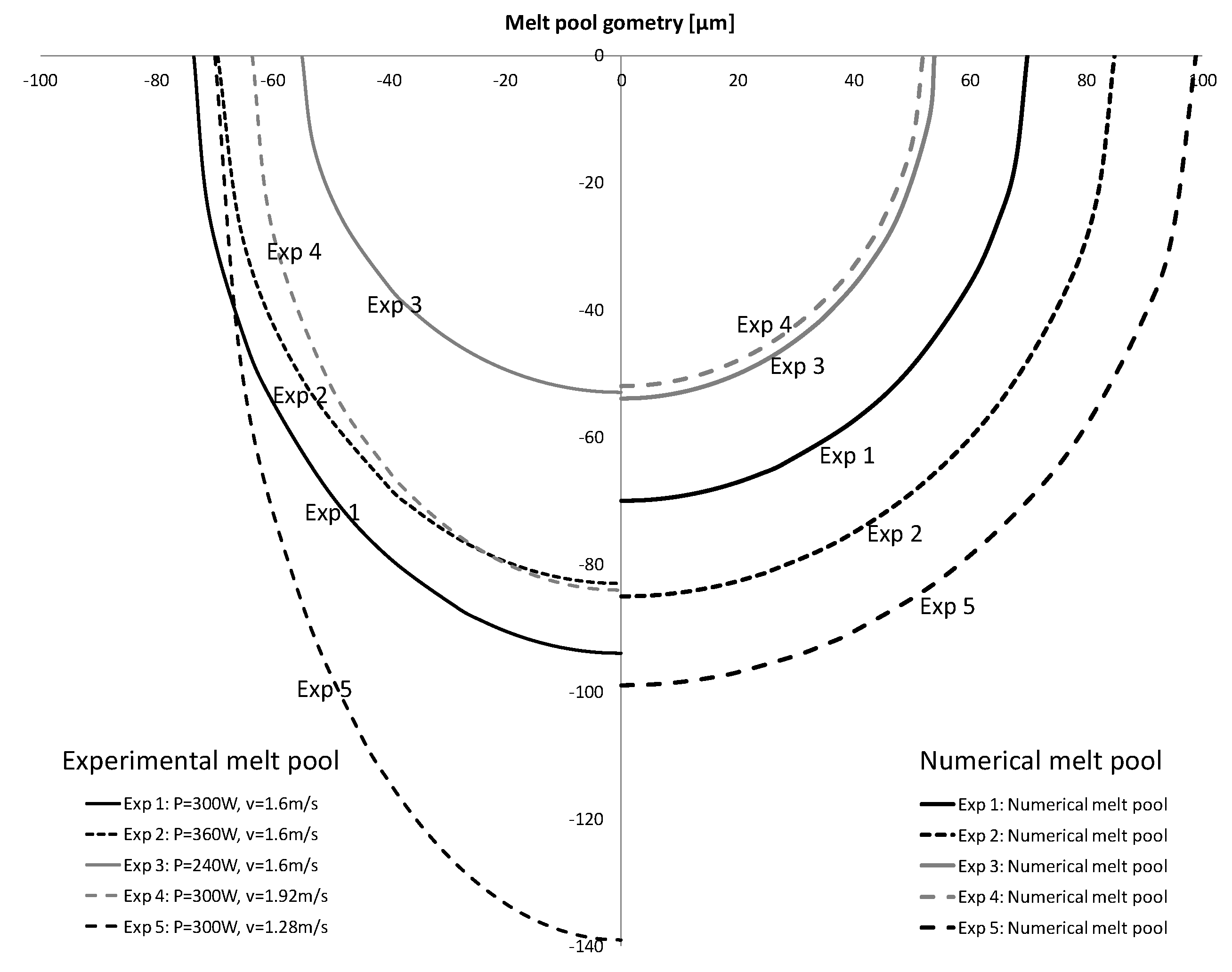
Using the data of the experiments and Equation (13) we performed a best fit, and estimated a characteristic time $t_c\left(\mathrm{s}\right)=0.121 \mathrm{s}$ and length ${\ell }_c=0.099 \mathrm{m}$. The numerically calculated radius is shown in the second to last row of Table 2. Out of the five sets of data, we obtained an excellent fit for two sets, a reasonable fit for the other two sets, and a poor fit for one data set among experimental and numerical results as illustrated in Figure 8 and Figure 9. The fact that our model required two fitted parameters, it was expected to fit at least two sets of data well. Although the fitting (Table 2) looks promising, a larger amount of experimental data is necessary in order to justify its applicability to an SLM process. For example, we used a far field temperature of $T_{\infty }=20 °\mathrm{C}$. However, temperature changed during the course of the experiment due to pre-heating, which occurred in the processed layer due the conduction during laser scanning of the adjacent powder (i.e., previously deposited and underlying beads). This was because in actual SLM there is no time for previous deposits and the substrate to cool down to room temperature before the current new bead is processed. Furthermore, the deviation from the circular shape, although it should be avoided for an SLM process, is a dominant effect in the experimental data. Finally, although the power of the laser was known, the total energy delivered to the melt pool was unknown (i.e., the duration of the laser scanning was not reported). Hence, although the results shown in Table 1 prove that the aforementioned model and assumptions could provide reliable results in a very efficient manner in terms of computation time, further controlled experiments are necessary in order to improve, justify, and extend the applicability of the model.

A comprehensive illustration of the results in Table 2 is provided in Figure 8. The numerical results of the melt pool cylindrical shape on the right of the figure are compared with the experimental measurements of the melt pool on the left of the figure for all five experiments.

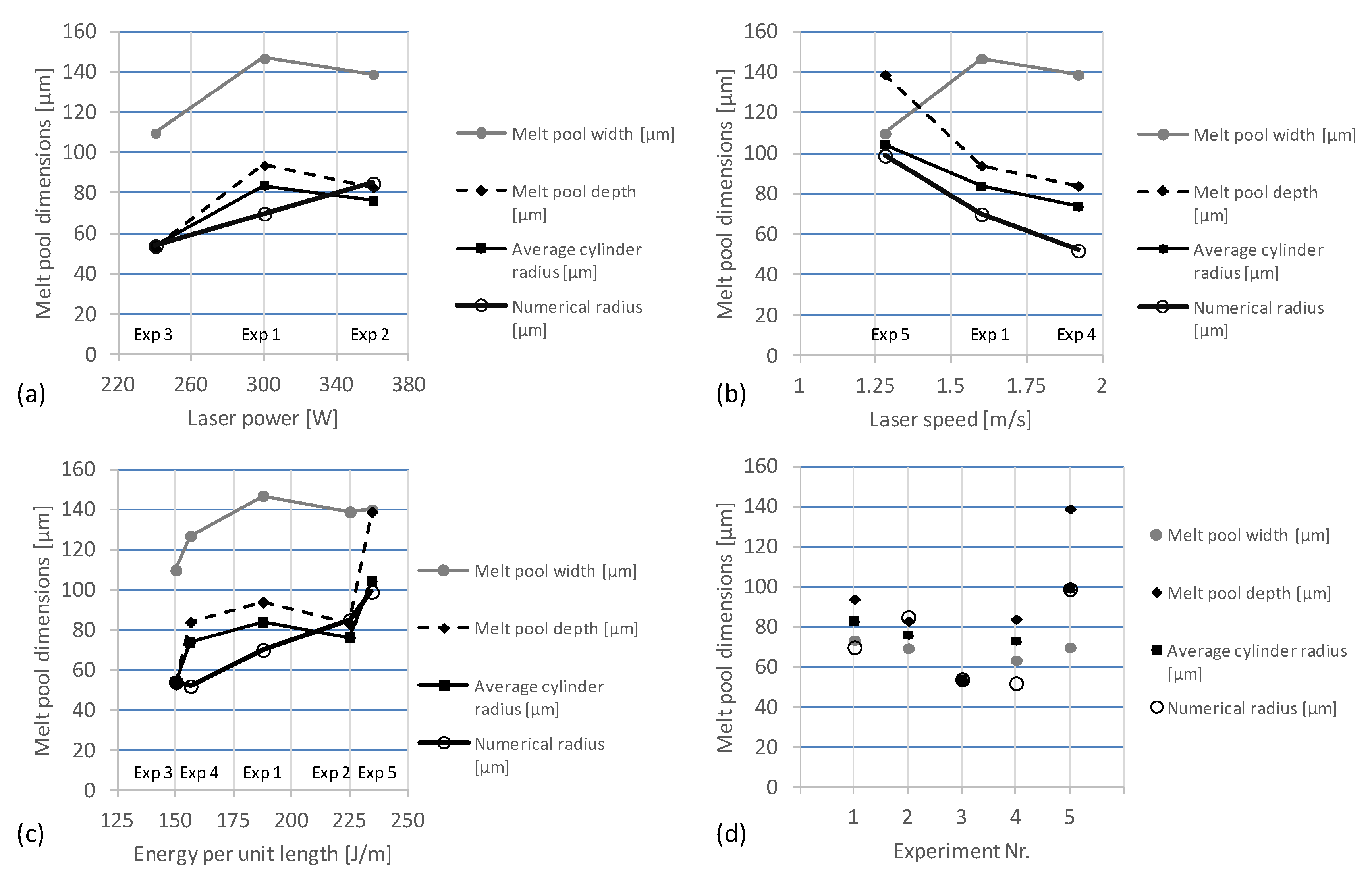
Figure 9 summarizes the numerical and experimental results of the melt pool dimensions in terms of the variation of (a) the laser power, (b) the laser speed, and (c) the energy per unit length. The results for all five experiments (d) demonstrate the deviation of the proposed analytical model compared to real melt pool dimensions.

5. Summary and Conclusions

We address the classical problem of a heat source activated along the span of a semi-infinite material. The material is solid (metal powder) and the melting commences immediately at the location of the line heat source due to the singular nature of the heat input. The temperature profile is cylindrically symmetric and the liquid-solid interface propagates radially outwards. The contribution of the current work is that we have included convection effects due to the density difference between the solid (metal powder) and the liquid (molten powder). Because the liquid has higher density than the powder, an annulus is developed with a radially-symmetric flow field; at small times we neglect gravitational and Marangoni effects. We show analytically that the convection enhances the melting speed and it is relatively important. We also show that if the properties of both the liquid and the solid phases of the material are varied by 10%, that does not affect significantly the results, hence constant properties can be used in numerical simulations. An important result of this work; however, is that, for a fixed amount of input energy per unit length, there exists an optimum combination of power input and time period of activation of the line heat source, which would lead to a maximum radius of the liquid-solid interface (i.e., a maximum amount of material would have melted during the activation time).

Finally, we use the analysis of the heat source per unit length to model an SLM process. We show that the point heat source associated with an SLM process can be represented with an equivalent heat source per unit length using an experimentally-determined characteristic time and length. The benefit of using a heat source model of this kind is twofold. On one hand, a rapid in-process computation of the melt pool can be achieved which can facilitate a real-time process parameter observation and optimization within the feasible process window, and on the other hand it can be applied for process control purposes during the SLM process. Additionally, such a simplified heat source model can be transferred comfortably in a subsequent thermo-mechanical model for computation of the structural shape and residual stresses. A comparison with experimental results has shown that the numerical results could provide a quantitative description of the process. However, further experiments are necessary in order to determine the conditions of applicability of the analytical model.

References

1. Carslaw, H.H.; Jaeger, J.C. Conduction of Heat in Solids; Oxford University Press: Oxford, UK, 1959; p. 296. [Google Scholar]
2. Paterson, S. Propagation of a boundary of fusion. Proc. Glasgow Math. Assoc. 1952, 1, 42–47. [Google Scholar] [CrossRef]
3. Hu, H.; Argyropoulos, A.S. Mathematical modelling of solidification and melting: A review. Model. Simul. Mater. Sci. Eng. 1996, 4, 371–396. [Google Scholar] [CrossRef]
4. Alexiades, V.; Lunardini, V.J.; Solomon, A.D. Mathematical Modeling of Melting and Freezing Processes. J. Sol. Energy Eng. 1993, 115, 121. [Google Scholar] [CrossRef]
5. Özişik, M.N. Heat Conduction; John Wiley & Sons: Hoboken, NJ, USA, 1980; p. 402. [Google Scholar]
6. Font, F.; Myers, T.G.; Mitchell, S.L. A mathematical model for nanoparticle melting with density change. Microfluid. Nanofluidics 2014, 18, 233–243. [Google Scholar] [CrossRef]
7. Eller, A. Rectified Diffusion during Nonlinear Pulsations of Cavitation Bubbles. J. Acoust. Soc. Am. 1965, 37, 493–503. [Google Scholar] [CrossRef]
8. Plesset, M.S.; Zwick, S.A. A Nonsteady Heat Diffusion Problem with Spherical Symmetry. J. Appl. Phys. 1952, 23, 95. [Google Scholar] [CrossRef]
9. Brenner, P.B.; Hilgenfeldt, S.; Lohse, D. Single bubble sonoluminescence. Rev. Mod. Phys. 2002, 74, 425–484. [Google Scholar] [CrossRef]
10. Chu, S.; Prosperetti, A. History effects on the gas exchange between a bubble and a liquid. Phys. Rev. Fluids 2016, 1, 1. [Google Scholar] [CrossRef]
11. Fyrillas, M.M.; Szeri, A.J. Dissolution or growth of soluble spherical oscillating bubbles. J. Fluid Mech. 1994, 277, 381. [Google Scholar] [CrossRef]
12. Cheng, B.; Chou, K. Melt Pool Evolution Study in Selective Laser Melting. In Proceedings of the 26th Annual International Solid Freeform Fabrication Symposium, Austin, TX, USA, 10–12 August 2015; Bourell, D.L., Ed.; University of Texas: Austin, TX, USA, 2015; pp. 1182–1194. [Google Scholar]
13. MERLIN Project. Development of Aero Engine Component Manufacture using Laser Additive Manufacturing, 7th Framework Programme FP7; Rolls-Royce plc: Derby, UK, 2013. [Google Scholar]
14. Polivnikova, T. Study and Modelling of the Melt Pool Dynamics during Selective Laser Sintering and Melting. Ph.D. Thesis, Ecole Polytechnique Federale de Lausanne, Lausanne, Switzerland, 2015. [Google Scholar]
15. Li, Y.; Zhou, K.; Tor, S.B.; Chua, C.K.; Leong, K.F. Heat transfer and phase transition in the selective laser melting process. Int. J. Heat Mass Transf. 2017, 108, 2408–2416. [Google Scholar] [CrossRef]
16. Letenneur, M.; Kreitcberg, A.; Brailovski, V. Optimization of Laser Powder Bed Fusion Processing Using a Combination of Melt Pool Modeling and Design of Experiment Approaches: Density Control. J. Manuf. Mater. Process. 2019, 3, 21. [Google Scholar] [CrossRef]
17. Li, Y.; Zhou, K.; Tan, P.; Tor, S.B.; Chua, C.K.; Leong, K.F. Modeling temperature and residual stress fields in selective laser melting. Int. J. Mech. Sci. 2018, 136, 24–35. [Google Scholar] [CrossRef]
18. Tan, P.; Shen, F.; Li, B.; Zhou, K. A thermo-metallurgical-mechanical model for selective laser melting of Ti6Al4V. Mater. Des. 2019, 168, 107642. [Google Scholar] [CrossRef]
19. Doumanidis, C. Simulation for control of sequential and scanned thermal processing. Int. J. Modeling Simul. 1997, 17, 169–177. [Google Scholar] [CrossRef]
20. Doumanidis, C.; Fourligkas, N. Temperature Distribution Control in Scanned Thermal Processing of Thin Circular Parts. IEEE Trans. Control Syst. Technol. 2001, 9, 708–717. [Google Scholar] [CrossRef]
21. Doumanidis, C.; Hardt, D.E. Simultaneous in-process control of heat-affected zone and cooling rate during arc welding. Weld. Res. Suppl. 1990, 69, 186–196. [Google Scholar]
22. Kruth, J.P.; Duflou, J.; Mercelis, P.; Van Vaerenbergh, J.; Craeghs, T.; De Kuester, J. On-line monitoring and process control in selective laser melting and laser cutting. In Proceedings of the 5th Lane Conference, Laser Assisted Net Shape Engineering, Erlangen, Germany, 25–28 September 2007; pp. 23–37. [Google Scholar]
23. Doumanidis, C.C. Modeling and Control of Timeshared and Scanned Torch Welding. J. Dyn. Syst. Meas. Control 1994, 116, 387–395. [Google Scholar] [CrossRef]
24. Papadakis, L.; Loizou, A.; Risse, J.; Bremen, S.; Schrage, J. A Computational Reduction Model for Appraising Structural Effects in Selective Laser Melting Manufacturing: A Methodical Model Reduction Proposed for Time-Efficient Finite Element Analysis of Larger Components in Selective Laser Melting. J. Virtual Phys. Prototyp. 2014, 9, 17–25. [Google Scholar] [CrossRef]
25. Doumanidis, C.; Fyrillas, M.; Polychronopoulou, K.; Ioannou, Y. Analytical model for geometrical characteristics control of laser sintered surfaces. Int. J. Nanomanuf. 2010, 6, 300. [Google Scholar]
26. Panton, L.P. Incompressible Flow; John Wiley & Sons: Hoboken, NJ, USA, 2005. [Google Scholar]
27. Davis, J.R. ASM Specialty Handbook: Heat-Resistant Materials; ASM International: Geauga County, OH, USA, 1997. [Google Scholar]
28. Hosaeus, H.; Seifter, A.; Kaschnitz, E.; Pottlacher, G. Thermophysical Properties of Solid and liquid Inconel 718. Alloy. High Temp. High Press. 2001, 33, 405–410. [Google Scholar] [CrossRef]
29. Shi, X.; Ma, S.; Liu, C.; Chen, C.; Wu, Q.; Chen, X.; Lu, J. Performance of High Layer Thickness in Selective Laser Melting of Ti6Al4V Materials. Materials 2016, 9, 975. [Google Scholar] [CrossRef] [PubMed]
Figure 1. Heat source (light gray color) of strength Q ˙ ( W / m ) distributed along the inner surface of the molten material as power per unit length.
Jmmp 03 00062 g001
Figure 2. A semi-infinite slab of fusible material melts cylindrically due to a heat source Q ˙ ( W / m ) . The temperature field is cylindrically symmetric. The uniformly cylindrical power distribution from the laser source (gray color) is assumed over the inner surface of the molten material with radius Ri.
Jmmp 03 00062 g002
Figure 3. Liquid-solid phase distribution for IN718 powder shown on the basis of the enthalpy change as a function of temperature based on data from [27,28].
Jmmp 03 00062 g003
Figure 4. The characteristic Equation (13) as a function of the eigenvalue λ . The root is at the point where F [ λ ] = 0 (i.e., λ = 0.255 ) .
Jmmp 03 00062 g004
Figure 5. Temperature distribution as a function of radius r from the cylinder center with a melt pool radius of 0.12 mm at time t = τ . The power per unit length is set to Q ˙ = 10000   W / m .
Jmmp 03 00062 g005
Figure 6. Radius of the melted material at time t = τ , as a function of power per unit length. The energy per unit length is constant Q = Q ˙ · τ = 150   J / m .
Jmmp 03 00062 g006
Figure 7. Macrographs of five selective laser melting (SLM) experiments with varying process parameters [13].
Jmmp 03 00062 g007
Figure 8. Comparison of the numerical melt pool cylindrical shape (right) vs. the measured melt pool dimensions (left) for the five sets of experiments.
Jmmp 03 00062 g008
Figure 9. Numerical vs. experimental results of the melt pool dimensions with varying laser power (a), laser speed (b), and energy per unit length (c). The deviation of the proposed analytical model compared to real melt pool dimensions for all five experiments is summarized in (d).
Jmmp 03 00062 g009