Energy Optimal Trajectory Planning for the Morphing Solar-Powered Unmanned Aerial Vehicle Based on Hierarchical Reinforcement Learning

Abstract

Trajectory planning is crucial for solar aircraft endurance. The multi-wing morphing solar aircraft can enhance solar energy acquisition through wing deflection, which simultaneously incurs aerodynamic losses, complicating energy coupling and challenging existing planning methods in efficiency and long-term optimization. This study presents an energy-optimal trajectory planning method based on Hierarchical Reinforcement Learning for morphing solar-powered Unmanned Aerial Vehicles (UAVs), exemplified by a Λ-shaped aircraft. This method aims to train a hierarchical policy to autonomously track energy peaks. It features a top-level decision policy selecting appropriate bottom-level policies based on energy factors, which generate control commands such as thrust, attitude angles, and wing deflection angles. Shaped properly by reward functions and training conditions, the hierarchical policy can enable the UAV to adapt to changing flight conditions and achieve autonomous flight with energy maximization. Evaluated through 24 h simulation flights on the summer solstice, the results demonstrate that the hierarchical policy can appropriately switch its bottom-level policies during daytime and generate real-time control commands that satisfy optimal energy power requirements. Compared with the minimum energy consumption benchmark case, the proposed hierarchical policy achieved 0.98 h more of full-charge high-altitude cruise duration and 1.92% more remaining battery energy after 24 h, demonstrating superior energy optimization capabilities. In addition, the strong adaptability of the hierarchical policy to different quarterly dates was demonstrated through generalization ability testing.

1. Introduction

High-altitude solar-powered Unmanned Aerial Vehicles (UAVs) rely on solar cells mounted on their wings to power the propulsion system, onboard electronic equipment, and other payloads. Due to their ability to achieve diurnal energy cycling, they are capable of sustained flight in the stratosphere for tens or even hundreds of hours [1]. These UAVs are characterized by strong endurance, high cruising altitudes, and wide operational ranges, which make them widely used in both military and civilian applications, such as communication relays, airborne early warning, and ground reconnaissance [2]. Considering the long-term and high-cost investments required for the development of advanced photovoltaic cells and energy storage batteries, planning trajectories to maximize solar energy utilization has become a cost-effective and convenient way to enhance the flight performance of high-altitude solar-powered UAVs [3].

Because of the inherent conditions of photovoltaic cell efficiency, high-altitude solar-powered UAVs face the problem of low energy harvesting efficiency in environments with limited solar radiation. Typical scenarios include dates approaching winter, or twilight periods containing dawn and dusk during daylight hours at any season, where phenomena such as low solar altitude angles and diminished solar irradiance power are prevalent. To address this challenge, the Aurora Flight Sciences Odysseus aircraft proposes a multi-wing morphing configuration design as a technical solution. During nocturnal operations, the UAV adopts a straight-wing configuration to increase aspect ratio, thereby reducing induced drag and electrical energy consumption [4]. In daylight flight phases, it optimizes solar incidence angles on outer wing surfaces through wing deflection mechanisms, effectively enhancing solar irradiance absorption efficiency. However, the morphing process can also cause some complications, such as suboptimal incidence angles of sunlight on partial wings, shadows caused by deflection, reducing effective illuminated surface area, and diminished effective lift-generating area with increasing deformation angles. These factors deepen the coupling relationship between energy consumption and energy absorption, thereby increasing the complexity of trajectory planning for such solar-powered UAVs.

1.1. Existing Research on Trajectory Planning for Solar-Powered Aircraft

Considering the optimal energy target, the flight trajectory optimization of high-altitude solar-powered UAVs is a complex problem that involves multiple constraints such as solar irradiance, atmospheric wind fields, flight attitude, and mission requirements. Ignoring the impact of wind fields, current research on UAV trajectory optimization mainly focuses on two aspects [5]. On the one hand, studies have focused on the incident angle of solar radiation on photovoltaic panels during flight, aiming to optimize flight attitude for greater solar energy harvesting. Klesh et al. [6] were among the first to investigate the path optimization problem of solar-powered UAVs. They discussed in detail the effects of bank angle and velocity on energy absorption and proposed a dimensionless power ratio parameter. Using the maximum principle, they predicted the qualitative characteristics of the aircraft’s energy optimization. In the three-dimensional (3D) aspect, Spangelo et al. [7] constrained the operational space of the solar-powered UAV to a vertical cylindrical surface and proposed an optimization method using periodic spline functions to solve the 3D trajectory of the UAV. Huang et al. [8] also restricted the flight platform on a cylindrical surface, transforming the three-dimensional space into a two-dimensional surface. They then disregarded the path within the cylinder and evaluated the impact of lateral motion on solar energy acquisition. Ailon [9] utilized differential flatness to plan a constant-altitude flight trajectory for a solar-powered UAV. This method does not require solving the nonlinear differential equations that arise from the dynamics and energy models, and it allows for real-time updates to the energy-optimal path. On the other hand, there is exploration of energy management strategies based on large-scale altitude changes, which aim to reduce the reliance of solar aircraft on batteries through gravitational energy storage. Gao et al. [10] studied an energy management strategy for solar-powered UAVs to convert solar energy into gravitational potential energy for storage. This strategy divides the day-night flight into three stages. In the first stage, the UAV stores solar energy in both batteries and gravitational potential. In the second stage, it releases gravitational potential energy through gravitational gliding. In the third stage, it relies on batteries for energy supply. Simulation results show that this strategy can effectively improve the remaining battery energy after the day-night flight. Ma et al. [11] researched the variable altitude flight trajectory and its application effects for solar aircraft based on the principle of gravitational energy storage, described the specific components of the variable altitude trajectory and the movement patterns of each part, established physical and mathematical models for the trajectory and time nodes of each part, and proposed a general parameter design method for solar aircraft applicable to the variable altitude trajectory. In addition, Marriott et al. [12], comprehensively considering the changes in altitude and attitude angle, introduced a greedy algorithm with buffering to plan the optimal 24-h energy flight trajectory of solar-powered aircraft in cylindrical space, which boasts faster computation speed, with only 1.5 min required for optimizing the flight trajectory every 30 min. Sun et al. [13] took into account the mission altitude constraint and divided the energy management strategy (EMS) of the solar aircraft into five stages: night-time low-altitude flight, maximum power ascent to mission altitude, level flight at mission altitude, maximum power ascent altitude, and longest endurance glide. They solved the optimal flight attitude in each stage separately. Compared to the existing EMS, the new EMS can store about 22.9% of the remaining energy, which is equivalent to reducing the weight of the rechargeable battery from 16.0 kg to 12.3 kg. Ni et al. [14] implemented deep reinforcement learning technology to enhance energy optimization. By holistically considering flight attitude parameters and gravitational potential energy storage mechanisms in their reward function design and employing the Soft Actor-Critic (SAC) algorithm for trajectory planning model training, their approach significantly improves the residual battery energy level after a 24 h flight of the solar-powered aircraft.

While existing studies predominantly focus on solar-powered UAVs with conventional configurations, preliminary studies have been conducted on multi-wing morphing configuration solar aircraft. For morphing aircraft, Montalvo [15] initially conducted a detailed study on the dynamic characteristics of multiple fixed-wing aircraft after wingtip docking and achieved the corresponding attitude control and trajectory tracking control. An et al. [16] conducted stability analysis on wingtip docking aircraft and studied its stabilization control. Zhou et al. [17] developed an attitude control system based on PID for the aircraft after wingtip docking. In the field of trajectory planning for morphing solar aircraft, Wang et al. [18] studied the three-dimensional path planning of a wing tip docking combined solar aircraft under mission constraints, focusing on exploring the optimal path of the aircraft in separation mode, but lacking consideration for the angle between the two wings in the combined state. Wu et al. [19,20,21] investigated solar-powered UAVs with multiple morphing configurations, demonstrating that appropriate wing deflection strategies under cross-latitude and cross-seasonal conditions can enhance solar energy harvesting. Their work also computed sun-tracking trajectories for morphing UAVs pursuing maximum solar irradiance. Li et al. [22] established an integrated modeling framework incorporating the communication link models, the solar irradiance prediction model, and the mass estimation model for a triple-fuselage configuration solar aircraft. By considering communication mission constraints and energy equilibrium constraints, their heuristic algorithm-based simulation analysis revealed that morphing design can reduce total airframe mass by 12–15%. Ma et al. [23] addressed the issue of weak solar radiation intensity in winter by changing the deflection angle of the winglet to enhance solar energy absorption and calculated the optimal deflection angle.

1.2. Existing Research on Trajectory Planning Based on Deep Reinforcement Learning

Based on a review of existing research on trajectory planning of solar-powered aircraft, their methods can be broadly categorized into two types. The first category involves offline trajectory optimization over the entire flight mission duration. The resulting strategy is fixed and predetermined, making it unable to adapt to uncertain conditions encountered mid-flight. Consequently, these methods cannot meet the adaptive requirements for uncertain environments, such as the Gaussian Pseudospectral Method (GPM) [24] and the direct collocation method using SNOPT computation [8]. The second category enables real-time trajectory computation through iterative calculations within finite horizons using flight data and idealized environmental models. However, its continuous re-planning process suffers from excessive computational load and low solving efficiency, as exemplified by the Model Predictive Control (MPC) method [25]. Morphing-configuration solar-powered UAVs, compared to conventional configurations, possess more complex models, which further accentuate the problems faced by both aforementioned categories of methods. Moreover, existing research on their trajectory planning considering energy constraints has only attempted direct numerical solutions or heuristic algorithms, leaving a lack of exploration into planning methods that can ensure real-time capability.

Deep Reinforcement Learning (DRL) possesses both powerful long-term planning capability and real-time decision-making ability. This stems from its value function incorporating the long-term rewards of actions, and its policy network structure resembling state feedback control. Furthermore, the deep neural network module it contains also exhibits powerful non-linear representation capability. Owing to these aforementioned advantages, DRL has been extensively applied in the field of aircraft trajectory planning in recent years. Pandian et al. [26], focusing on the UAV trajectory planning problem with energy constraints, conducted a comprehensive comparison between on-policy algorithms (TRPO, PPO) and off-policy algorithms (DQN, DDPG, TD3, SAC). The simulation results indicated that off-policy algorithms capable of addressing continuous action spaces, particularly SAC and TD3, demonstrated superior performance in optimizing energy consumption while ensuring mission completion. Chen et al. [27] proposed an energy-efficient path planning method based on reinforcement learning for the multi-target path planning problem of quadrotor UAVs in turbulent wind environments. In each iteration, the predicted energy consumption of the discrete path is incorporated into the neural network’s observations. Simulation results show that this method outperforms traditional algorithms such as SAC and TD3 in terms of reward gain and robustness in complex turbulent environments. Li et al. [28] proposed a novel Quantum-inspired Experience Replay (QiER) framework for DRL-based navigation tasks in cellular-connected drones, which associates the importance of experienced transition with its associated quantum bit and applies amplitude amplification technology based on Grover iteration. The DRL-QiER solution demonstrated effectiveness and excellence in numerical results.

Some researchers have also made preliminary attempts to utilize DRL to address trajectory planning problems that consider energy harvesting from the environment. Reddy [29] employed a reinforcement learning approach, incorporating wind field information and aerodynamic parameters into the observations, to guide an agent learning from extensive real flight data spanning several days. This agent enabled a glider to devise navigation strategies that effectively utilize updrafts. References [14,30], using conventional solar-powered UAVs as the flight platform, adopted a reinforcement learning framework based on the SAC algorithm to investigate 24 h energy-optimal trajectory planning strategies, analyzing scenarios with and without considering wind fields.

1.3. The Potential of Hierarchical Reinforcement Learning

Traditional DRL methods still exhibit certain shortcomings when applied to the trajectory planning of solar-powered UAVs. To enable a trained agent to plan a 24 h trajectory achieving energy loop closure, a whole day of environmental information, including solar irradiance, is required as training data. The sheer volume of this data can make it difficult for neural networks of limited scale to fully extract the hidden features within the flight information, potentially leading to underfitting issues. For instance, the agent’s performance reported in reference [14] did not fully adhere to the designed reward structure. Hierarchical Reinforcement Learning (HRL) decomposes the problem on the basis of DRL and is better able to adapt to complex environments or large-scale tasks [31]. Currently, the application of HRL in trajectory planning and flight decision-making has been explored. Chai et al. [32] applied HRL to air combat problems, modeling the UAV’s air combat decision-making process as two loops. The outer loop determines macro strategies based on the current combat situation, while the inner loop generates flight commands according to the macro strategy. Both controllers are trained using the PPO algorithm, demonstrating superior air combat strategy tracking capabilities and higher win rates compared to traditional methods. Lv et al. [33] proposed a flight hierarchical trajectory planning framework based on the TD3 algorithm, which decomposes airship tasks into two layers: the long-range path planning task and the short-range path planning task. The effectiveness of the framework is verified through simulated flights in forecasted wind fields. In addition, references [34,35,36] also explored the applications of HRL in UAV path planning and flight decision-making. The typical 24 h trajectory of a solar-powered UAV exhibits distinct phase characteristics. By setting different policies, potentially corresponding to these phases, HRL can address the challenge posed by the large volume of 24 h data. Therefore, generating 24 h trajectory planning policies for solar-powered UAVs using HRL is a method worth exploring.

1.4. Work of This Study

In summary, this study will focus on the energy-optimal trajectory planning problem for morphing configuration solar-powered UAVs, adopting HRL as the design method for its trajectory planning policy. The specific research will be carried out based on a Λ-shaped aircraft, aiming to achieve both real-time performance and aircraft energy optimization during trajectory generation.

The main contributions of this study are as follows:

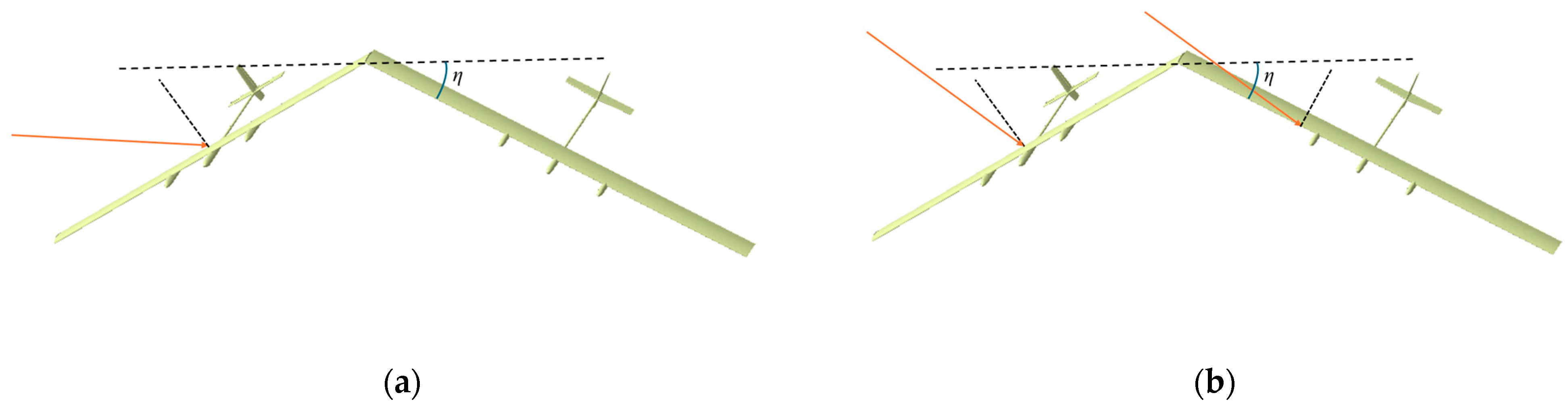
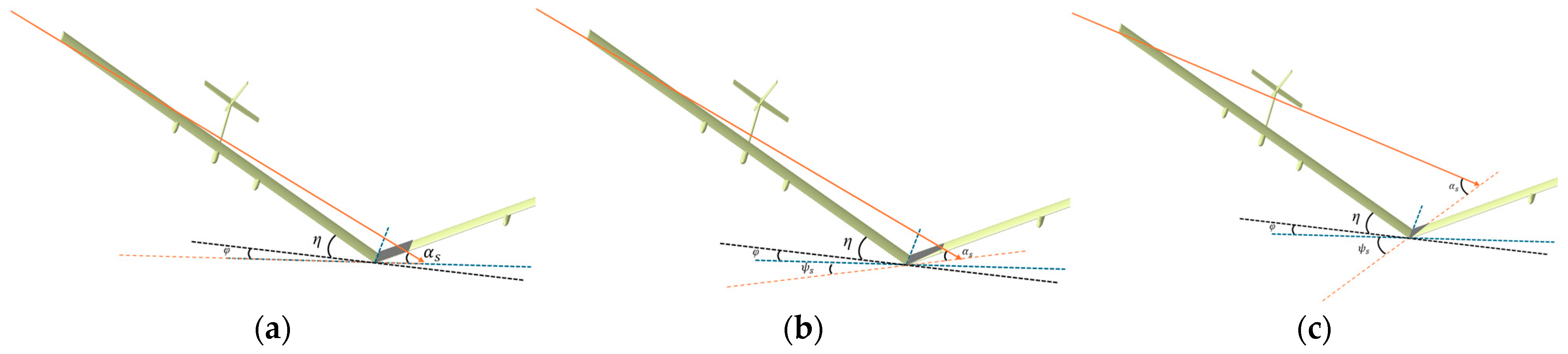
• The simulation mathematical model for the Λ-shaped morphing solar-powered UAV is established, including its aerodynamic model, dynamics and kinematics model, solar energy absorption model, and energy storage and consumption model. These provide a modeling foundation for its trajectory planning.
• Based on the phased characteristics of the 24 h trajectory of solar-powered UAVs, a classification method for the operating conditions of the Λ-shaped solar-powered UAV during 24 h flight is proposed with energy as the reference. On the basis of classification, HRL is employed to address the energy-optimal trajectory planning problem for the UAV, and a complete hierarchical policy training process is designed.
• The trajectory planning policy based on HRL can adaptively respond to different flight operating conditions within a 24 h period. Based on flight information, it outputs appropriate real-time commands for thrust, attitude angles, and wing deflections, thereby continuously tracking the peak energy power and maintaining the optimal energy state.

The remainder of this paper is organized as follows. Section 2 details the simulation model of the Λ-shaped solar-powered UAV. Section 3 describes the method for dividing the operating conditions of the Λ-shaped solar-powered UAV during a 24 h flight. Section 4 introduces the principle of the HRL algorithm based on the Option Framework and the trajectory planning model based on HRL. Section 5 provides a detailed introduction to the key design for training the hierarchical trajectory planning policy. Section 6 evaluates the performance of the HRL-based policy through simulated flight and compares it with a benchmark method. Finally, Section 7 summarizes the main findings of this paper and suggests directions for future research.

2. Model

The mathematical models of the Λ-shaped UAV used in this work include the aerodynamic model, dynamics and kinematics model, inner loop response model, solar irradiation model, solar energy absorption model, and energy consumption and storage model, which are described in detail as follows.

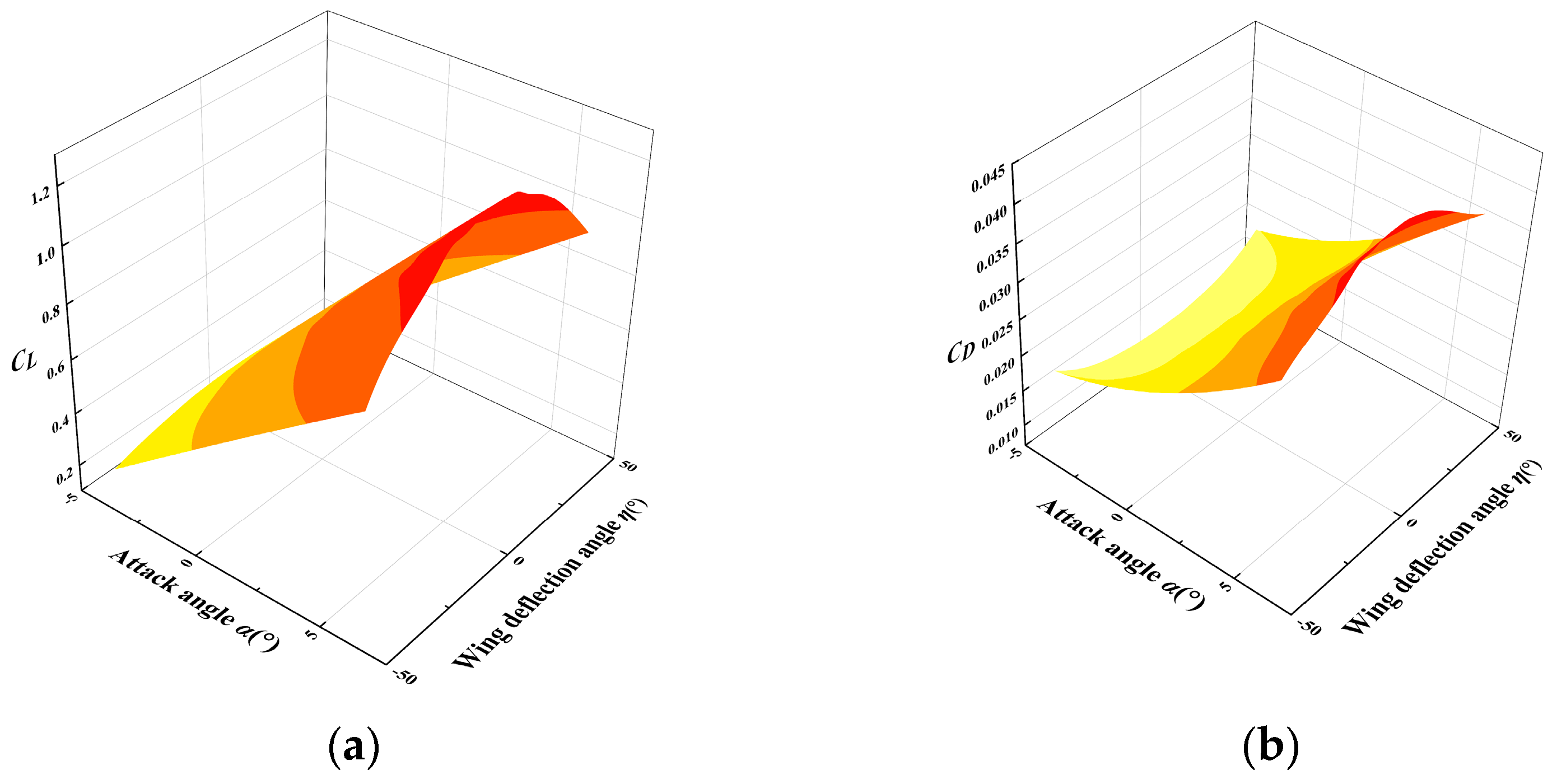
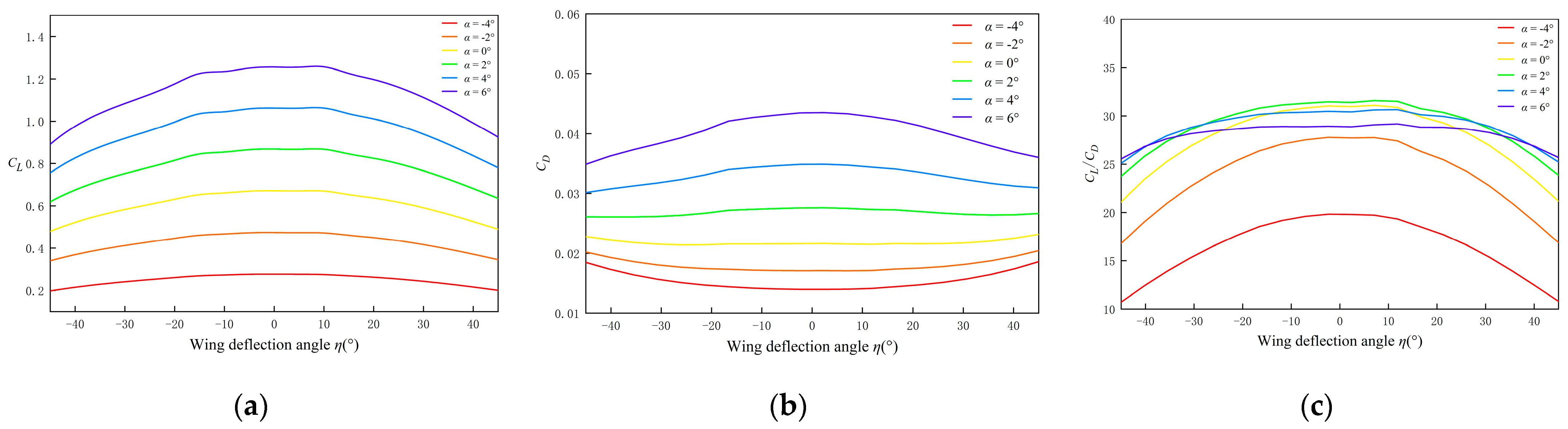
2.1. The Aerodynamic Model

In this study, the Λ-shaped UAV draws on the scheme in reference [21], which is formed by joining two conventional configuration solar-powered UAVs at their wingtips. It can adjust its attitude and the angle between its wing surfaces (inter-wing angle) while flying in the stratosphere to track solar irradiation based on its current position and time. The wingtip connection is achieved through a hinge, and the change in the inter-wing angle is achieved by adjusting the wing deflection. To focus on the trajectory planning problem, this study treats the connection as an ideal rotatable mechanism, which is a common assumption in existing research in this field [19]. Due to the symmetrical configuration of the Λ-shaped aircraft, this paper defines the magnitude of the wing deflection angle η as half the supplementary angle of the angle between the two wings. Upward deflection is considered positive, while downward deflection is considered negative. Figure 1 shows the UAV with η of 0° and 20°.

The aerodynamic coefficients of the UAV at different wing deflection angles are calculated using the open-source simulation software OpenVSP v.3.32.2. The simulation is carried out using the vortex lattice method, and to reduce errors, the attack angle range is limited to −4° to 6°, with the sideslip angle not considered. Selected conditions of attack angle and wing deflection angle are used to calculate the lift coefficient $C_L$ and drag coefficient $C_D$. The obtained results are provided in Appendix A. The interpolation of these results reveals the relationship between aerodynamic coefficients and both attack angle α and wing deflection angle η, as illustrated in Figure 2.

To intuitively analyze the aerodynamic characteristics of the Λ-shaped UAV, several specific attack angles are selected, and curves showing the variation of its lift coefficient, drag coefficient, and lift-to-drag ratio with wing deflection angle are presented, as shown in Figure 3a–c. It can be observed that when the attack angle is positive, the larger the absolute value of the wing deflection angle, the smaller the drag coefficient, and conversely, the smaller the absolute deflection angle, the larger the drag coefficient. However, regardless of whether the attack angle is positive or negative, the larger the absolute value of the wing deflection angle, the smaller both the lift coefficient and the lift-to-drag ratio become. Depending on the attack angle, the deflection angle range where the maximum lift coefficient or maximum lift-to-drag ratio occurs is approximately −2° to 10°. The above phenomenon is consistent with the research results of the existing studies on the influence of wing dihedral angle on aerodynamic performance [37,38]. This indicates that if solely considering the achievement of good aerodynamic efficiency, the UAV should avoid its wing deflection as much as possible.

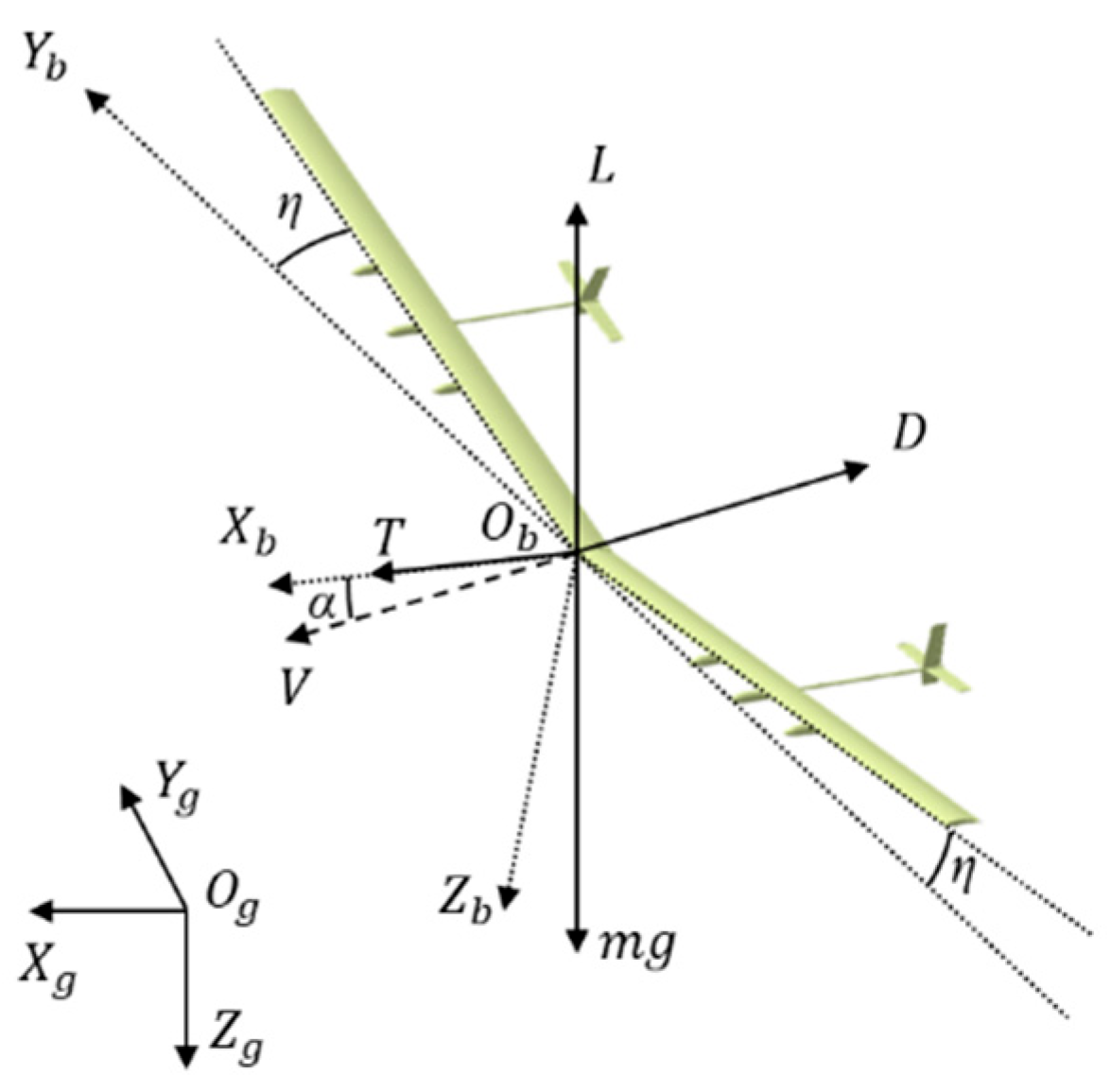
2.2. The Dynamic and Kinematic Model

In large-scale trajectory planning, the aircraft can be treated as a mass point. Therefore, this paper employs a simplified 3-DOF particle model. The effects of the sideslip angle and installation angle of the propulsion system are neglected. Meanwhile, since the morphing solar-powered UAV is designed for application in the stratosphere, where the atmosphere is thin and the wind field gradient is minimal, having little impact on centroid dynamics, this study also neglects the effects of weather and the wind field. The coordinate system for the Ʌ-shaped UAV is shown in Figure 4, where $O_g{X}_g{Y}_g{Z}_g$ represents the north-east-down inertial coordinate system, and $O_b{X}_b{Y}_b{Z}_b$ is the body coordinate system. $O_b{X}_b$ points towards the front of the aircraft, $O_b{Y}_b$ towards the right wingtip at $0^{°}$ wing deflection angle, and $O_b{Z}_b$ points downwards. Previous studies have calculated the wingtip angle based on the bank angle of each sub aircraft [15], but in this study, as described in Section 2.1, due to the symmetrical configuration of the Ʌ-shaped UAV, calculating using the wing deflection angle and the overall aircraft bank angle is equivalent to using the bank angles of two sub aircrafts. The bank angle of the overall aircraft depends on the relationship between the body coordinate system and the inertial coordinate system.

Through force analysis, the kinematic and dynamic equations for the Ʌ-shaped UAV are obtained as follows [39]:

$$\left\{\begin{array}{c}\begin{array}{c}\dot{V}={\displaystyle \frac{1}{m}}\left(T\mathrm{c}\mathrm{o}\mathrm{s}\alpha -D-mg\mathrm{s}\mathrm{i}\mathrm{n}\gamma \right)\\ \dot{\gamma }={\displaystyle \frac{1}{mV}}\left[\left(T\mathrm{s}\mathrm{i}\mathrm{n}\alpha +L\right)\mathrm{c}\mathrm{o}\mathrm{s}\phi -\mathrm{m}\mathrm{g}\mathrm{c}\mathrm{o}\mathrm{s}\gamma \right]\\ \dot{\psi }={\displaystyle \frac{1}{mV\mathrm{c}\mathrm{o}\mathrm{s}\gamma }}\left[\left(T\mathrm{s}\mathrm{i}\mathrm{n}\alpha +L\right)\mathrm{s}\mathrm{i}\mathrm{n}\phi \right]\end{array}\\ \begin{array}{c}\dot{x}=V\mathrm{c}\mathrm{o}\mathrm{s}\gamma \mathrm{c}\mathrm{o}\mathrm{s}\psi \\ \dot{y}=V\mathrm{c}\mathrm{o}\mathrm{s}\gamma \mathrm{s}\mathrm{i}\mathrm{n}\psi \\ \dot{z}=-V\mathrm{s}\mathrm{i}\mathrm{n}\gamma \end{array}\\ \begin{array}{c}L={\displaystyle \frac{1}{2}}\rho V^2{f}_L\left(\alpha , \eta \right)S_r\\ D={\displaystyle \frac{1}{2}}\rho V^2{f}_D\left(\alpha , \eta \right)S_r\end{array}\end{array}\right.,$$

(1)

where V represents the airspeed, γ is the trajectory inclination angle, ψ is the yaw angle, x, y, and z are the positions of the aircraft in the inertial coordinate system, α is the attack angle, which is the angle between $O_b{X}_b$ and the velocity vector, φ is the bank angle, m is the total mass, g is the acceleration due to gravity, which is 9.8 m/s², $S_r$ is the aerodynamic reference area, which varies with η, while $f_L$ and $f_D$ are the interpolation functions for the lift and drag coefficients, respectively, determined by α and η. Additionally, the pitch angle θ can be calculated as follows:

$$\theta =\gamma +\alpha ,$$

(2)

The thrust T, lift L, and drag D are the forces acting on the aircraft. Here, T is generated by the propulsion system, parallel to the $O_b{X}_b$ axis and in the same direction. L and D arise from the airflow, with L perpendicular to the airspeed vector and D parallel to the airspeed vector but in the opposite direction.

2.3. The Ideal Inner-Loop Response Model

For the dynamic process of generating control commands for the UAV to track the trajectory, an ideal inner-loop controller is selected to simplify the problem. For a given command, the proportional feedback control mechanism based on the preset time scale $t_a$ is adopted to calculate the command response u at the current moment, as described below:

$$\left\{\begin{array}{c}{t}_a{\displaystyle \frac{du}{dt}}=u_d-u\\ u_d=u_0+∆u_{cmd}\end{array}\right.,$$

(3)

In the response process of control commands, $u_d$ represents the expected value of different types of control commands, $u_0$ is the initial state of the control command, and $∆u_{cmd}$ is the numerical increment of the control command. According to Equation (1), control commands for the UAV during trajectory planning should be T, α, φ, and η.

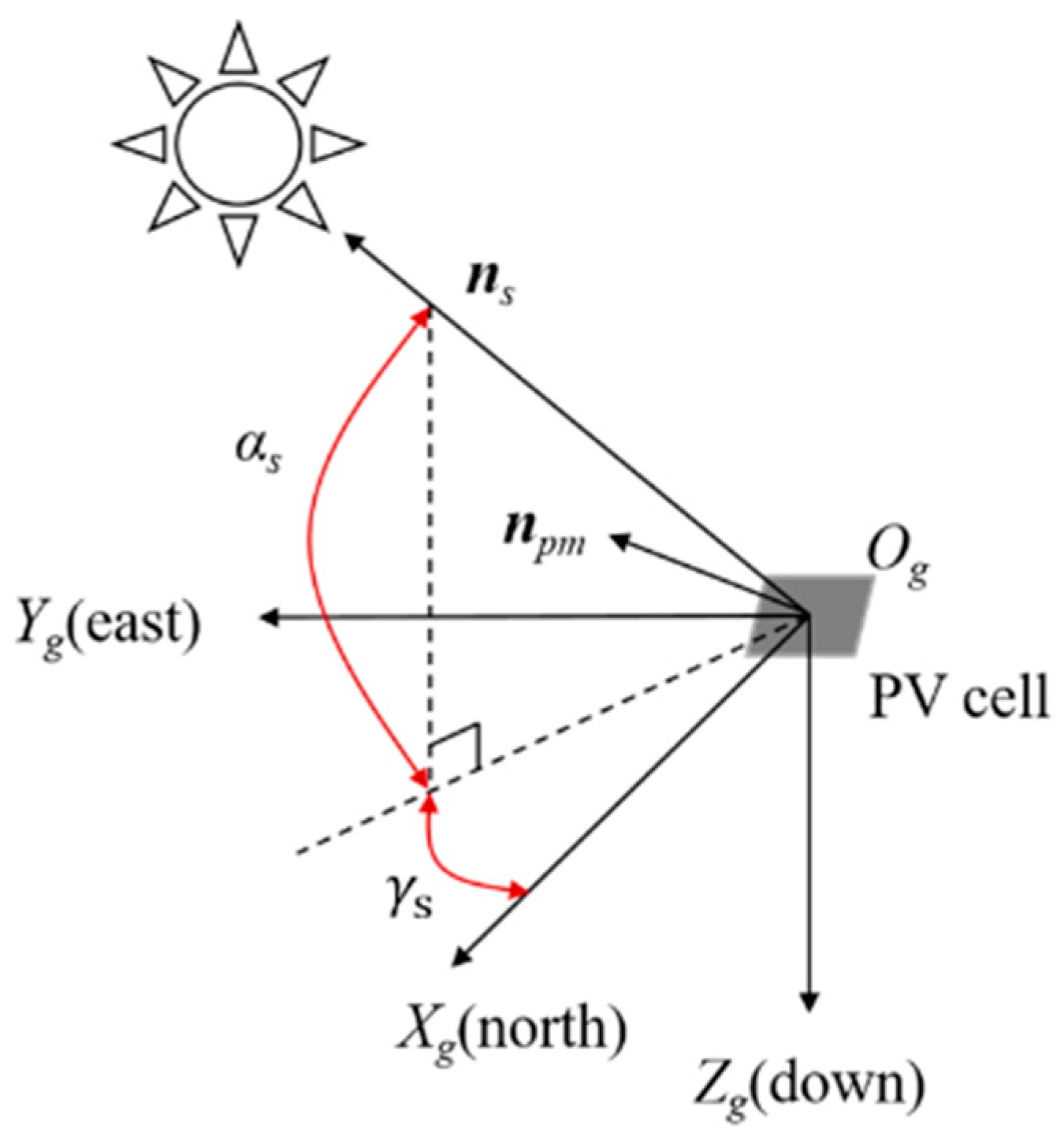
2.4. The Solar Irradiation Model

This study adopts the mathematical model introduced by B. Keidel et al. [40] for real-time calculation of solar radiation information. The incident angle of sunlight on a photovoltaic (PV) cell is shown in Figure 5, where ${\alpha }_s$ is the solar altitude angle, ${\gamma }_s$ is the solar azimuth angle, $n_s$ points from the center of the PV cell to the sun, and $n_{pm}$ is perpendicular to the PV cell.

During flight in the stratosphere, due to the thinness of clouds and the scarcity of impurities in the atmosphere, the impact of reflected radiation can be neglected. Therefore, the solar radiation received by the PV cell can be categorized into two types. One type is direct radiation $I_{dir}$, which travels directly from the sun to the photovoltaic cell. The other type is scattered radiation $I_{diff}$, which is scattered repeatedly by the atmosphere before reaching the photovoltaic cell. Hence, the expression for the total radiation $I_{tot}$ is as follows:

$$I_{tot}=I_{dir}+I_{diff},$$

(4)

where $I_{dir}$ can be expressed as:

$$I_{dir}=I_{on}\mathrm{e}\mathrm{x}\mathrm{p}\left(-{\displaystyle \frac{0.375\mathrm{e}\mathrm{x}\mathrm{p}\left(-h/7\right)}{{\mathrm{s}\mathrm{i}\mathrm{n}\left(\frac{{\alpha }_s+{\alpha }_{dep}}{1+{\alpha }_{dep}/90}\right)}^{0.678+h/40}}}\right),$$

(5)

and $I_{diff}$ can be calculated by the following equation:

$$I_{diff}=0.08I_{dir}\mathrm{e}\mathrm{x}\mathrm{p}(-h/7),$$

(6)

where h is the altitude, $I_{on}$ is the exoatmospheric solar irradiance on the $n_d$ day of the year, and ${\alpha }_{dep}$ is the corrected value of ${\alpha }_s$ relative to the ground. They can be calculated by the following equations:

$$\left\{\begin{array}{c}{I}_{on}=G_{sc}\left[1+0.033\mathrm{c}\mathrm{o}\mathrm{s}\left(360n_d/365\right)\right]\\ {\alpha }_{dep}=0.57+\mathrm{arc}\cos \left[R_{earth}/\left(R_{earth}+h\right)\right]\end{array}\right.,$$

(7)

Among Equation (7), $G_{sc}$ is the standard solar radiation constant, which is 1367 W/m², and $R_{earth}$ is Earth’s radius, 6357 km.

2.5. The Energy Absorption Model

For the i-th PV cell with an area of $S_{PV}^i$, its solar irradiance flux can be calculated using $n_{pm}$ and $n_s$, and the expression is as follows:

$${\Phi }_i=I_{tot}{S}_{PV}^i\mathrm{c}\mathrm{o}\mathrm{s}(n_s,n_{pm}),$$

(8)

Ignoring the installation angle of the PV cell on the wing upper surface, when there is no wing deflection angle, $n_s$ and $n_{pm}$ can be expressed using the aircraft attitude angle, solar azimuth angle ${\gamma }_s$, and solar altitude angle ${\alpha }_s$, with their expressions as follows [40]:

$$\left\{\begin{array}{c}{n}_s={\left[-\mathrm{c}{\mathrm{o}\mathrm{s}\alpha }_s\mathrm{c}\mathrm{o}\mathrm{s}{\gamma }_s,-\mathrm{c}\mathrm{o}\mathrm{s}{\alpha }_s\mathrm{s}\mathrm{i}\mathrm{n}{\gamma }_s,-\mathrm{s}\mathrm{i}\mathrm{n}{\alpha }_s\right]}^T\\ n_{pm}=-\left[\begin{array}{c}\cos \psi \sin \theta \cos \phi +\sin \psi \sin \phi ;\\ \sin \psi \sin \theta \cos \phi -\cos \psi \sin \phi ;\\ \cos \theta \cos \phi \end{array}\right]\end{array}\right.,$$

(9)

When there is a wing deflection angle η, the normal vectors of the PV cells on the upper surface of the left or right wing are represented as follows:

$$\left\{\begin{array}{c}{n}_{pm,left}=-\left[\begin{array}{c}\cos \psi \sin \theta \cos \left(\phi +\eta \right)+\sin \psi \sin \left(\phi +\eta \right);\\ \sin \psi \sin \theta \cos \left(\phi +\eta \right)-\cos \psi \sin \left(\phi +\eta \right);\\ \cos \theta \cos (\phi +\eta )\end{array}\right]\\ n_{pm, right}=-\left[\begin{array}{c}\cos \psi \sin \theta \cos \left(\phi -\eta \right)+\sin \psi \sin \left(\phi -\eta \right);\\ \sin \psi \sin \theta \cos \left(\phi -\eta \right)-\cos \psi \sin \left(\phi -\eta \right);\\ \cos \theta \cos (\phi -\eta )\end{array}\right]\end{array}\right.,$$

(10)

It is assumed that the onboard PV cells of the Λ-shaped solar-powered UAV are symmetrically and uniformly distributed on its left and right wings. Substituting Equation (10) into Equation (8) yields the following expression for the solar irradiation flux on the i-th pair of PV cells:

$${\Phi }_i=I_{tot}{S}_{PV}^i\left(\mathrm{c}\mathrm{o}\mathrm{s}\right(n_s,n_{pm,left})+\mathrm{c}\mathrm{o}\mathrm{s}(n_s,n_{pm,right}\left)\right),$$

(11)

When $\mathrm{c}\mathrm{o}\mathrm{s}(n_s,n_{pm,left})$ or $\mathrm{c}\mathrm{o}\mathrm{s}(n_s,n_{pm,right})$ is less than 0, it signifies that the corresponding wing upper surface faces away from the sun and cannot receive solar irradiation. Furthermore, it may potentially shadow the illuminated area of the other wing’s upper surface. When the wing deflection angle η ≤ 0, the illumination situation is shown in Figure 6, where (b) indicates that a wing upper surface facing completely away from the sun does not obstruct the illuminated area of the other wing. When the wing deflection angle η > 0, let ${\psi }_s$ be the angle between the horizontal projection of the sunlight vector and the line perpendicular to the horizontal projection of $O_b{X}_b$, which can be calculated by (ψ − ${\gamma }_s$ − 90°). As $\left|\mathrm{t}\mathrm{a}\mathrm{n}\left({\psi }_s\right)\right|$ increases, the illuminated area of the sun-receiving wing surface gradually increases, as shown in Figure 7.

Let S be the reference area of the upper surface of a single wing, l be the span of a single wing, and c be the wing chord length. According to Figure 7a–c, when the right wing surface is backlit and the left wing surface is illuminated, the gray area on the left wing surface represents the shadow caused by the occlusion of the right wing. Therefore, the expression for the illuminated area S′ of the left wing surface is as follows:

$$\left\{\begin{array}{c}if \left|\tan {\psi }_s\right|=0, S_1^{\prime }=(1-{\displaystyle \frac{\mathrm{s}\mathrm{i}\mathrm{n}(\eta -(\phi +{\alpha }_s\left)\right)}{\mathrm{s}\mathrm{i}\mathrm{n}(\eta +(\phi +{\alpha }_s\left)\right)}})S \\ if l{\displaystyle \frac{\mathrm{s}\mathrm{i}\mathrm{n}(\eta -(\phi +{\alpha }_s\left)\right)}{\mathrm{s}\mathrm{i}\mathrm{n}(\eta +(\phi +{\alpha }_s\left)\right)}}\cos \left(\eta +\phi \right)\left|\mathrm{t}\mathrm{a}\mathrm{n}{\psi }_s\right|\le c, S_2^{\prime }=S_1^{\prime }+0.5l^2{\left({\displaystyle \frac{\mathrm{s}\mathrm{i}\mathrm{n}(\eta -(\phi +{\alpha }_s\left)\right)}{\mathrm{s}\mathrm{i}\mathrm{n}(\eta +(\phi +{\alpha }_s\left)\right)}}\right)}^2\cos \left(\eta +\phi \right)\left|\mathrm{t}\mathrm{a}\mathrm{n}{\psi }_s\right|\\ if l{\displaystyle \frac{\mathrm{s}\mathrm{i}\mathrm{n}(\eta -(\phi +{\alpha }_s\left)\right)}{\mathrm{s}\mathrm{i}\mathrm{n}(\eta +(\phi +{\alpha }_s\left)\right)}}\cos \left(\eta +\phi \right)\left|\mathrm{t}\mathrm{a}\mathrm{n}{\psi }_s\right|>c, S_3^{\prime }=S_1^{\prime }-{\displaystyle \frac{0.5c^2}{\cos \left(\eta +\phi \right)\left|\mathrm{t}\mathrm{a}\mathrm{n}{\psi }_s\right|}}\end{array}\right.$$

(12)

The progression of the three conditions in Equation (12) represents the UAV’s heading transitioning from being completely perpendicular to the solar irradiation direction to gradually facing the solar irradiation direction, thereby causing the shadow area on the left wing to gradually decrease. Similarly, when the left wing surface is backlit and the right wing surface is illuminated, the expression for the illuminated area S′ of the right wing surface is as follows:

$$\left\{\begin{array}{c}if \left|\tan {\psi }_s\right|=0, S_1^{\prime }=(1-{\displaystyle \frac{\mathrm{s}\mathrm{i}\mathrm{n}(\eta +(\phi -{\alpha }_s\left)\right)}{\mathrm{s}\mathrm{i}\mathrm{n}(\eta -(\phi -{\alpha }_s\left)\right)}})S \\ if l{\displaystyle \frac{\mathrm{s}\mathrm{i}\mathrm{n}(\eta +(\phi -{\alpha }_s\left)\right)}{\mathrm{s}\mathrm{i}\mathrm{n}(\eta -(\phi -{\alpha }_s\left)\right)}}\cos \left(\eta -\phi \right)\left|\mathrm{t}\mathrm{a}\mathrm{n}{\psi }_s\right|\le c, S_2^{\prime }=S_1^{\prime }+0.5l^2{\left({\displaystyle \frac{\mathrm{s}\mathrm{i}\mathrm{n}(\eta +(\phi -{\alpha }_s\left)\right)}{\mathrm{s}\mathrm{i}\mathrm{n}(\eta -(\phi -{\alpha }_s\left)\right)}}\right)}^2\cos \left(\eta -\phi \right)\left|\mathrm{t}\mathrm{a}\mathrm{n}{\psi }_s\right|\\ if l{\displaystyle \frac{\mathrm{s}\mathrm{i}\mathrm{n}(\eta +(\phi -{\alpha }_s\left)\right)}{\mathrm{s}\mathrm{i}\mathrm{n}(\eta -(\phi -{\alpha }_s\left)\right)}}\cos \left(\eta -\phi \right)\left|\mathrm{t}\mathrm{a}\mathrm{n}{\psi }_s\right|>c, S_3^{\prime }=S_1^{\prime }-{\displaystyle \frac{0.5c^2}{\cos \left(\eta -\phi \right)\left|\mathrm{t}\mathrm{a}\mathrm{n}{\psi }_s\right|}}\end{array}\right.$$

(13)

Summarizing the above, the expression for the solar energy absorption power of the Λ-shaped solar-powered UAV is as follows:

$$\left\{\begin{array}{c}if \eta >0 \mathrm{and} {\alpha }_s<\left|\phi \right| \mathrm{and} \cos \left(n_s,n_{pm,left}\right)<0 \mathrm{and} \cos \left(n_s,n_{pm,right}\right)>0,\\ P_{solar}={\displaystyle \frac{S^{\prime }}{S}}{\displaystyle \sum _i}{\eta }_{MPPT}{\eta }_{PV}{I}_{tot}{S}_{PV}^i\left(\cos \left(n_s,n_{pm,right}\right)\right)\\ else if \eta >0 \mathrm{and} {\alpha }_s<\left|\phi \right| \mathrm{and} \cos \left(n_s,n_{pm,left}\right)>0 \mathrm{and} \cos \left(n_s,n_{pm,right}\right)<0,\\ P_{solar}={\displaystyle \frac{S^{\prime }}{S}}{\displaystyle \sum _i}{\eta }_{MPPT}{\eta }_{PV}{I}_{tot}{S}_{PV}^i\left(\cos \left(n_s,n_{pm,left}\right)\right)\\ else P_{solar}={\displaystyle \sum _i}{\eta }_{MPPT}{\eta }_{PV}{I}_{tot}{S}_{PV}^i(\cos \left(n_s,n_{pm,left}\right)+\cos \left(n_s,n_{pm,right}\right))\end{array}\right.$$

(14)

where $S_{PV}^i$ represents the area of one cell from the i-th pair of photovoltaic cells, ${\eta }_{PV}$ is the efficiency of the PV cell, and ${\eta }_{MPPT}$ is the efficiency of the Maximum Power Point Tracking (MPPT). The solar energy absorption power is 0 when the cosine of the angle between $n_s$ and $n_{pm}$ for the PV cell is negative.

2.6. The Energy Consumption Model

The propulsion system and avionics generate the main energy consumption during the flight of the Ʌ-shaped UAV [41], so the required power $P_{need}$ can be determined as Equation (15).

$$\left\{\begin{array}{c}{P}_{prop}={\displaystyle \frac{TV}{{\eta }_{prop}{\eta }_{mot}}}\\ P_{need}=P_{prop}+P_{acc}\end{array}\right.,$$

(15)

where T is the thrust, V is the flight velocity, ${\eta }_{prop}$ is the efficiency of the propeller, ${\eta }_{mot}$ is the efficiency of the motor, $P_{prop}$ is the required power for the propulsion system, and $P_{acc}$ is the required power for the avionics.

2.7. The Energy Storage Model

The net power of the battery $P_{battery}$ depends on the solar energy absorption power $P_{solar}$ and the required power $P_{need}$ [42]. The percentage of the remaining battery charge relative to its maximum storage capacity represents the current battery energy state of the UAV, referred to as the State of Charge (SOC). Its rate of change, which depends on $P_{battery}$, is shown in Equations (17) and (18).

$$P_{battery}=P_{solar}-P_{need},$$

(16)

$$SOC={\displaystyle \frac{E_{battery}}{E_{battery,max}}},$$

(17)

$$\dot{SOC}=\left\{\begin{array}{c}{\displaystyle \frac{\dot{E_{battery}}}{E_{battery,max}}}={\displaystyle \frac{P_{battery}}{E_{battery,max}}}, SOC<100\%\\ {\displaystyle \frac{P_{battery}}{E_{battery,max}}} or 0, SOC=100\%\end{array}\right.,$$

(18)

where $E_{battery}$ is the current battery energy, $E_{battery,max}$ is the maximum battery energy. When the battery is not fully charged, the rate of change in SOC is proportional to $P_{battery}$. When the battery remains fully charged, the rate of change in $E_{battery}$ is 0, then the rate of change in SOC is 0. During the fully charged period, $\dot{SOC}$ is non-zero only in two critical states: when the battery is just fully charged or when it starts to discharge from the fully charged state.

In addition to battery energy, gravitational potential energy is another form of energy storage for the UAV, which can be released through unpowered gliding. The expression for the gravitational potential energy stored by the aircraft is shown in (19), where $h_0$ is set as the initial takeoff altitude of the aircraft.

$$E_{potential}=mg(h-h_0),$$

(19)

The parameters required for the aforementioned models are shown in

Table 1. The model parameters.

Parameter	Description	Value	Parameter	Description	Range
m (kg)	Aircraft mass	70	h (m)	Altitude	[15,000, 25,000]
Sr,0 (m2)	Reference area when η is 0°	31.84	R (m)	Flight radius	[0, 5000]
c (m)	Chord length	1.0272	V (m/s)	Airspeed	[15, 80]
l (m)	Wingspan of a single wing	15.1	T (N)	Thrust	[0, 100]
SPV (m2)	Solar panel area of a single wing	12	α (°)	Attack angle	[−4, 6]
Ebattery,max (kWh)	Maximum battery energy	16	φ (°)	Bank angle	[−5, 5]
Pacc (kW)	Avionics power	0.3	η (°)	Wing deflection angle	[−45, 45]
ηMPPT	MPPT efficiency	0.95	θ (°)	Pitch angle	[−15, 15]
ηPV	Solar panel efficiency	0.3	ψ (°)	Yall angle	[−180, 180]
ηprop	Propeller efficiency	0.82	SOC	State of Charge	[0.15, 1]
ηmot	Motor efficiency	0.9	${\alpha }_s$ (°)	Solar altitude angle	[−90, 90]
ta (s)	Inner loop response time	3.33	${\gamma }_s$ (°)	Solar azimuth angle	[−180, 180]

.

3. Minimum Energy Consumption Trajectory Analysis

This section will plan and analyze the minimum energy consumption benchmark trajectory of the Ʌ-shaped solar-powered UAV combined with gravity energy storage and attitude optimization, and then summarize the operating conditions faced by the Ʌ-shaped UAV during the 24 h flight, serving as the design basis for the hierarchical trajectory planning policy.

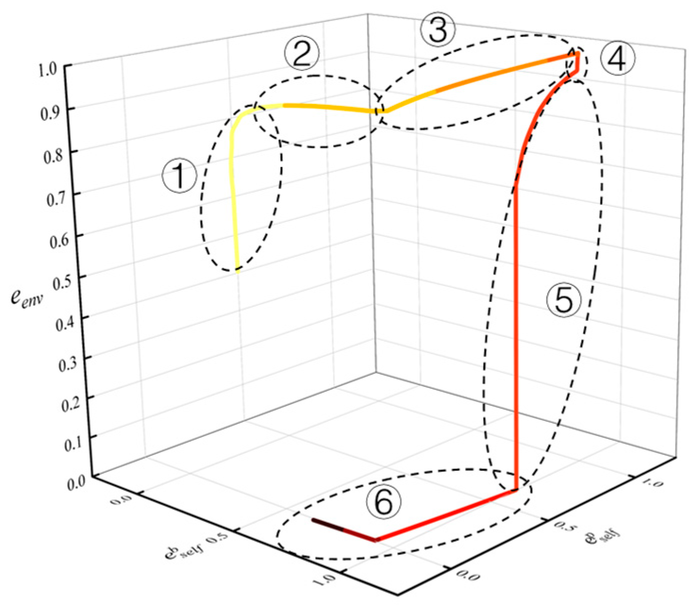
3.1. Minimum Energy Consumption State-Machine Policy

State-Machine policy is a widely adopted benchmark trajectory planning policy in the field. Guided by this policy, a UAV always maintains minimum energy consumption circling flight and changes its operations, such as cruising, climbing, and descending, according to certain rules.

The computation form for maintaining circling flight with the minimum energy consumption at any altitude of the Λ-shaped UAV is as follows:

$$\left\{\begin{array}{c}minimize { P}_{need}\\ with respect to V, T,\alpha ,\phi , \eta \\ \begin{array}{cc}subject to& \begin{array}{c}\dot{V}=0\\ \dot{\gamma }=0\\ \dot{\psi }={\displaystyle \frac{V}{R}}\end{array}\end{array}\end{array}\right.,$$

(20)

where R is the radius of circling flight, and γ determines whether the UAV is horizontal circling, circular climbing, or circular descending. This study sets the rules of the State-Machine policy as follows:

• Low-altitude charging cruising: The UAV cruises horizontally with minimum energy consumption power at the initial altitude until the SOC reaches a threshold.
• Climbing: After the SOC reaches the threshold, the UAV climbs until it reaches the maximum altitude or its SOC begins to decrease.
• High-altitude cruising: The UAV cruises horizontally at the end of the climbing until the SOC begins to decrease.
• Descent: The UAV descends to the lowest altitude.
• Low-altitude cruising: The UAV cruises horizontally after returning to the lowest altitude.

In order to comprehensively analyze the different states of the morphing solar-powered UAV, the summer solstice day with the largest range of solar altitude angle changes is selected as the simulation flight date. The minimum and maximum altitudes are based on the upper and lower limits of altitude in Table 1. The initial altitude is the same as the minimum altitude, the initial time is set to 4:24, which corresponds to sunrise, the initial SOC is set to 30%, and the flight location is (39.92° N, 116.42° E). The SOC threshold for initiating the climb is set to 95%, which is a common setting to reduce battery degradation from charging and discharging cycles. γ is 1.5° during climbing and −1.5° during descent, and R is 5000 m. The planned State-Machine benchmark trajectory is shown in Figure 8.

3.2. Classification of Flight Conditions

The stored energy and environmental energy of the UAV in this trajectory are analyzed. According to the energy storage model, the stored energy of the UAV itself includes battery energy $E_{battery}$ and gravitational potential energy $E_{potential}$. According to the energy absorption model, the solar energy absorption power $P_{solar}$ is related to the total solar radiation power $I_{tot}$, PV cell area, attitude angle, and wing deflection angle. Only $I_{tot}$ completely depends on natural factors such as altitude and time. Therefore, $I_{tot}$ at any time in the trajectory is used to represent the environmental energy of the UAV at that time. The total energy state at any time t in the trajectory can be expressed in vector form as follows:

$${\mathit{e}}_{\mathit{t}}={\left[e_{self}^b, e_{self}^p, e_{env}\right]}_t,$$

(21)

Among them, $e_{self}^b$ represents the UAV’s battery energy storage, which is equivalent to SOC. $e_{self}^p$ represents the UAV’s potential energy storage, and $e_{env}$ represents the external energy faced by the UAV, which are, respectively, normalized by $E_{potential}$ and $I_{tot}$. They are plotted as three-dimensional coordinates to obtain the total energy variation curve of the Ʌ-shaped UAV, as shown in Figure 9. The color from light to dark represents time from morning to night. This curve can be finely divided into six stages.

Stage ① lasts for about 1 h from sunrise to the first arrival of $e_{env}$ at about 0.86. In this stage, the solar altitude angle ${\alpha }_s$ is relatively low, and $I_{tot}$ faced by the UAV is weak, which means that the environmental energy is relatively scarce. $e_{self}^b$ remains relatively unchanged, indicating that the UAV has difficulty charging through solar radiation at this stage.

Stage ② lasts for about 3 h when $e_{env}$ ranges from 0.86 to about 0.96. During this stage, ${\alpha }_s$ and $I_{tot}$ gradually increase, and $e_{self}^b$ gradually rises to 0.95, representing that the UAV raises its SOC to the threshold through solar radiation charging.

Stage ③ lasts for about 5.3 h from the end of stage ② until $e_{self}^p$ reaches 1. During this stage, $e_{env}$ and $e_{self}^b$ reach and remain at their maximum values, while $e_{self}^p$ increases from 0 to 1, indicating that the UAV’s battery energy and environmental energy are sufficiently abundant to convert excess solar energy into gravitational potential energy, thereby increasing the UAV’s total energy storage.

Stage ④ lasts for about 4 h from the end of stage ③ to the beginning of the decrease in $e_{self}^p$. During this stage, $e_{self}^b$ and $e_{self}^p$ remain at their maximum values, while $e_{env}$ slightly decreases, indicating that ${\alpha }_s$ and $I_{tot}$ begin to diminish over time, but it does not affect the UAV’s ability to maintain its own energy storage.

Stage ⑤ lasts for about 1.5 h from the end of stage ④ until $e_{env}$ reaches 0. At this stage, $e_{self}^b$ has not reduced, while $e_{self}^p$ and $e_{env}$ have significantly decreased, indicating that the diminishing in ${\alpha }_s$ and $I_{tot}$ near sunset has affected the solar energy absorption of the UAV, causing it to release gravitational potential energy to maintain battery energy.

Stage ⑥ lasts for 9.2 h from the end of stage ⑤ until the end of the 24 h flight. At this stage, $e_{env}$ is 0, and both $e_{self}^b$ and $e_{self}^p$ gradually decrease. $e_{self}^p$ drops to 0 first compared to $e_{self}^b$, after that, the rate of decrease of $e_{self}^b$ rises significantly, indicating that the UAV can only consume its own stored energy and chooses to prioritize the consumption of stored gravitational potential energy to reduce the loss of battery energy.

Based on the changes in $e_{self}^b$, $e_{self}^p$, and $e_{env}$, the above six stages are summarized as three flight operating conditions that the Ʌ-shaped solar-powered UAV needs to face during 24 h flight. At the same time, the optimal flight strategy for the UAV in each operating condition is given.

Operating Condition 1: During daytime, solar irradiation is present, and the UAV’s battery energy is scarce. In this condition, the Λ-shaped solar-powered UAV needs to significantly enhance its solar irradiation absorption efficiency to shorten the time required to fully charge the battery. The UAV, in the trajectory shown in Figure 8, only flies with minimum energy consumption and does not consider utilizing wing deflection to improve solar energy absorption efficiency; consequently, it performs poorly in stage ①. For the Λ-shaped UAV, it should utilize wing deflection as much as possible to leverage its energy harvesting advantage in low solar altitude angle scenarios, provided that aerodynamic losses can be compensated.

Operating Condition 2: During daytime, solar irradiation is present, and the UAV’s battery energy is abundant. In this condition, the Λ-shaped solar-powered UAV needs to adopt a flight strategy that balances battery charge and gravitational potential energy. Gaining potential energy should not come at the expense of battery charge, and the duration of stage ⑤ should be shortened through appropriate wing deflection.

Operating Condition 3: During nighttime, there is no solar irradiation. In this condition, the UAV cannot harvest energy and needs to consistently fly with minimum energy consumption.

The aforementioned content is summarized as shown in

Table 2. Flight operating condition classification and optimization strategies.

Operation Condition	Stage	${\mathit{e}}_{\mathit{e}\mathit{n}\mathit{v}}$ > 0		${\mathit{e}}_{\mathit{e}\mathit{n}\mathit{v}}$ = 0		Energy Optimal Flight Strategies
		$\mathbf{Scare} {\mathit{e}}_{\mathit{s}\mathit{e}\mathit{l}\mathit{f}}^{\mathit{b}}$	$\mathbf{Abundant} {\mathit{e}}_{\mathit{s}\mathit{e}\mathit{l}\mathit{f}}^{\mathit{b}}$	$\mathbf{Scare} {\mathit{e}}_{\mathit{s}\mathit{e}\mathit{l}\mathit{f}}^{\mathit{b}}$	$\mathbf{Abundant} {\mathit{e}}_{\mathit{s}\mathit{e}\mathit{l}\mathit{f}}^{\mathit{b}}$
1	①②	√				Enhancing solar energy absorption efficiency at low solar altitude angles through wing deflection.
2	③④⑤		√			(1) Balancing battery energy and gravitational potential energy; (2) Shortening the duration of stage ⑤.
3	⑥			√		Minimum energy consumption flight.

. This table can provide guidance for the design and training of the hierarchical trajectory planning policy for the Λ-shaped UAV.

4. Hierarchical Reinforcement Learning

This section details an HRL algorithm based on an Options Framework and a Ʌ-shaped solar-powered UAV trajectory planning model that relies on this algorithm.

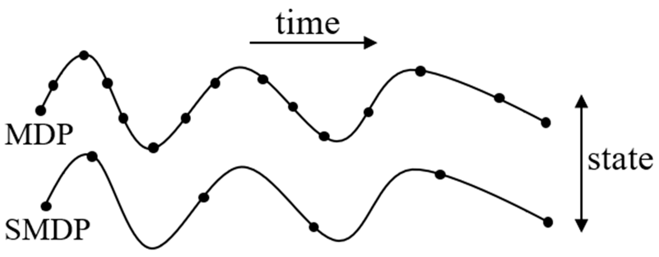
4.1. Option-Based HRL

The essence of HRL is to abstract complex long-term planning problems into different hierarchical levels, so as to solve them more effectively. In this study, the Options Framework [31], a method commonly used in HRL, is adopted. Next, the details of the Options Framework and the reason for selecting it will be introduced.

An option is a meaningful time series decision process, which can also be interpreted as a macro action performed over a duration. In a Markov Decision Process (MDP) with a given state set S and action set A, an option can be defined as a triple $(I, \pi ,\beta )$. Among them, $\pi :S\times A⟶[0, 1]$ represents the policy within the option, $\beta :S⟶[0, 1]$ denotes the termination condition, where $\beta \left(s\right)$ indicates the probability that the option terminates in state s, and $I\subseteq S$ is the initial state set of the option, which is available for state s only when $s\in I$. When the option starts executing, the agent selects actions through the intra-option policy $\pi$ until termination. To solve HRL problems using the Options Framework, the policy-over-option $\mu :S\times O_s⟶[0, 1]$ also needs to be defined, where $O$ represents the set of all options, and $O_s$ denotes the set of available options in state s. $\mu (s,o)$ indicates the probability of selecting o as the current option in state s.

Formally, a set of options defined on MDP constitutes the Semi-Markov Decision Process (SMDP), which provides the theoretical basis for the Option Framework. Based on the standard MDP, the state transition probability $P$ in the SMDP is expressed as $P(s^{,},\tau |s,a)$, which represents the probability that the transition time is $\tau$ when the action $a$ is executed in state s. In the SMDP, the action $a$ actually corresponds to the option o in the Option Framework.

The state trajectories of MDP and SMDP are shown in Figure 10. An option spans from $s_t$ to $s_{t+\tau }$. For every intermediate time in the interval $t\le k\le t+\tau$, the MDP is determined exclusively by $s_k$. In contrast, the SMDP may rely on the entire sequence of states. Applying SMDP to Q-learning, updates are carried out after each option ends with the formula given by:

$$Q\left(s,o\right)\leftarrow Q\left(s,o\right)+\alpha \left[r+{\gamma }^{\tau }{\displaystyle \genfrac{}{}{0pt}{}{max}{o^{\prime }\in O_{s^{\prime }}}}Q\left(s^{\prime },o^{\prime }\right)-Q\left(s,o\right)\right],$$

(22)

The flight trajectory of a UAV can essentially be described as the outcome of a sequence of discrete actions. As known from Section 3.2, the 24 h trajectory of the Ʌ-shaped solar-powered UAV exhibits distinct phased characteristics. In different stages, the UAV needs to adopt action sequences with different tendencies to obtain the maximum reward for the current phase. Therefore, its trajectory planning policy requires two capabilities. First, the ability to select an appropriate action sequence based on the current flight operating conditions. Second, the capability for the chosen action sequence to effectively guide the UAV towards acquiring the maximum energy return. This necessitates that the policy learns both the selection of action sequences and the selection of actions within those sequences. This aligns with the fundamental logic of the Options Framework in HRL algorithms. Consequently, the HRL trajectory planning method in this research is established based on the Options Framework.

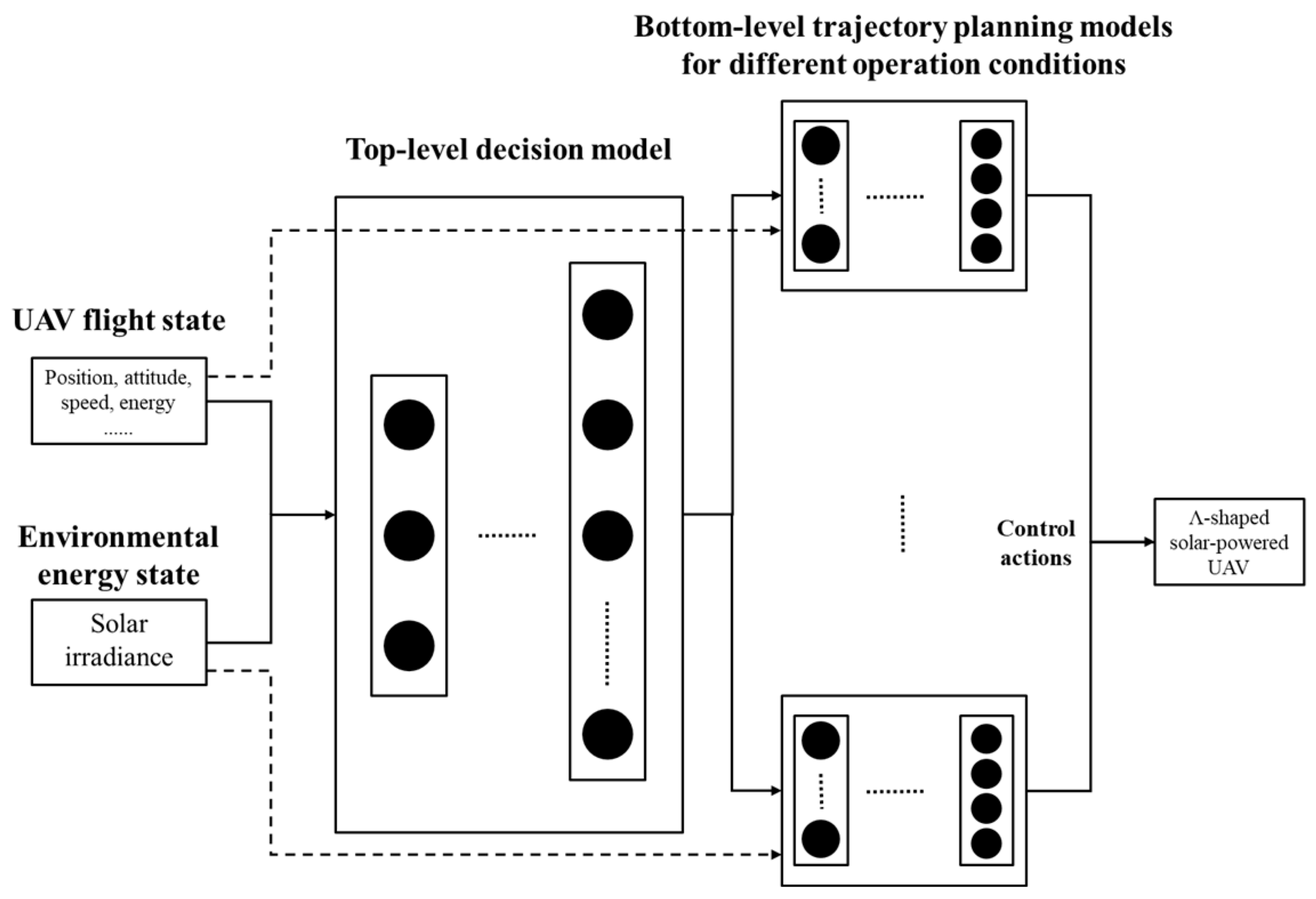
4.2. Option-Based Hierarchical Trajectory Planning Model

In general, in options-based HRL methods, it is necessary to simultaneously train the intra-option policies, the termination policy, and the policy-over-option. In the work presented in this research, the SMDP adopts a fixed number of steps. Each intra-option policy terminates after this fixed duration, at which point the policy-over-option chooses a new option. Consequently, the termination policy $\beta$ does not need to be updated. It is expressed in the following fixed form:

$${\beta }_k=\left\{\begin{array}{c}0, k<\tau \\ 1, k=\tau \end{array}\right.,$$

(23)

where $\tau$ denotes the fixed number of time steps in the SMDP, and the option will not terminate until it has been executed for $\tau$ steps.

Furthermore, adopting an integrated training approach presents challenges for the intra-option policies in learning logical action sequences, particularly for complex problems like trajectory planning. There is also a risk of overfitting individual actions instead of meaningful action sequences. Therefore, it is necessary to pre-train the intra-option policies using expert knowledge or experience. Consequently, this research adopts a fixed termination function and employs a sequential training approach, first training the intra-option policies and then the policy-over-option.

Based on the above, the hierarchical trajectory planning model for the Ʌ-shaped solar-powered UAV, founded on the Options Framework, is illustrated in Figure 11. The neural network of each bottom-level model, acting as an intra-option policy network, learns trajectory planning policies adapted to different flight operating conditions. Concurrently, the neural network of its top-level decision model, serving as the policy-over-option network, learns the option selection policy. The hierarchical policy can generate the energy-optimal trajectory adaptively for the UAV according to changes in flight operating conditions. By outputting control actions through the currently selected bottom-level policy network, it guides the UAV throughout its 24 h day-night flight mission.

5. Hierarchical Trajectory Planning Policy

Based on the results of the preceding benchmark trajectory analysis and the HRL-based trajectory planning model, this section details the design of the hierarchical policy, including the training algorithm, state space, action space, reward function, and training settings.

5.1. The Bottom-Level Policies

According to Table 2, the Ʌ-shaped solar-powered UAV encounters three flight operating conditions during its day-and-night flight. Consequently, corresponding bottom-level trajectory planning policies need to be designed for each type of operating condition to serve as intra-option policies, which enable the UAV to effectively pursue the optimal energy state.

On the basis of the mathematical model established in Section 2, the UAV’s flight information can be described by the state vector s, as shown in Equation (24). This vector includes its position, flight attitude, wing deflection, flight velocity, battery energy, solar angles, and control information.

$$\mathit{s}=[x,y,h,\phi ,\theta ,\psi ,\eta ,V,\alpha ,T,{\alpha }_s,{\gamma }_s,SOC],$$

(24)

Each bottom-level policy will define its state space by selecting appropriate components from the state vector s, tailored to the specific flight operating condition. To obtain finer trajectories, the bottom-level policies adopt continuous action spaces and are trained using the high-performance and stable SAC algorithm [43].

5.1.1. SAC Algorithm

SAC algorithm is a model-free reinforcement learning method and an off-policy algorithm. Its distinct feature from other algorithms lies in the simultaneous maximization of both the reward and the policy entropy. Introducing maximum entropy ensures that the policy remains as random as possible, allowing the agent to fully explore the state space, avoid premature convergence to a local optimum, and discover multiple feasible solutions to complete assigned tasks, thereby enhancing interference resistance. Additionally, to improve algorithm performance, techniques from Deep Q-Network (DQN) are adopted, including the introduction of two Q-networks and target networks. An adaptive temperature coefficient α is introduced to quantify the significance of entropy maximization. By tuning α for different scenarios, the problem is constructed as a constrained optimization task: maximizing expected returns while ensuring policy entropy remains above a predefined threshold. The pseudocode for the SAC algorithm is presented in Algorithm 1.

Algorithm 1. Soft Actor-Critic.

Input: ${\theta }_1, {\theta }_2, \phi$  ${\overline{\theta }}_1\leftarrow {\theta }_1$, ${\overline{\theta }}_2\leftarrow {\theta }_2$    $D\leftarrow \varnothing$  for each iteration do    for each environment step do      $a_t~{\pi }_{\phi }\left(a_t|s_t\right)$      $s_{t+1}~p\left(s_{t+1}|s_t,a_t\right)$      $D\leftarrow D\cup \left\{\left(s_t,a_t,r\left(s_t,a_t\right),s_{t+1}\right)\right\}$    end for    for each gradient step do      ${\theta }_i\leftarrow {\theta }_i-{\lambda }_Q{\widehat{\nabla }}_{{\theta }_i}{J}_Q\left({\theta }_i\right) \mathrm{f}\mathrm{o}\mathrm{r} i \in \left\{\mathrm{1,2}\right\}$      $\phi \leftarrow \phi -{\lambda }_{\pi }{\widehat{\nabla }}_{\phi }{J}_{\pi }\left(\phi \right)$      $\alpha \leftarrow \alpha -\lambda {\widehat{\nabla }}_{\alpha }J\left(\alpha \right)$      ${\overline{\theta }}_i\leftarrow \tau {\theta }_i+\left(1-\tau \right){\overline{\theta }}_i$ $for i \in \left\{\mathrm{1,2}\right\}$    end for  end for Output: ${\theta }_1, {\theta }_2, \phi$

5.1.2. The Bottom-Level Policy for Operating Condition 1

This policy needs to guide the Λ-shaped solar-powered UAV to enhance its solar energy absorption efficiency, thereby accelerating the charging rate. According to Equations (16)–(18), the rate of change of SOC before it reaches its maximum is directly proportional to the battery power. Therefore, the action reward for this policy at any given time t is designed as a dense reward function, formulated as follows:

$$r_t=P_{battery,t}=P_{solar,t}-P_{need,t},$$

(25)

Since the reward function is independent of SOC, the state space observed by this policy during its training is as follows:

$${\mathit{s}}_{\mathit{t}}=[x_t,y_t,h_t,{\phi }_t,{\theta }_t,{\psi }_t,{\eta }_t,V_t,{\alpha }_t,T_t,{\alpha }_{s,t},{\gamma }_t],$$

(26)

According to the inner-loop response model in Section 2.3, the action space for this policy consists of the thrust increment $∆T_{cmd}$, the attack angle increment $∆{\alpha }_{cmd}$, the bank angle increment $∆{\phi }_{cmd}$, and the wing deflection angle increment $∆{\eta }_{cmd}$. Considering the physical constraints of the UAV, the value ranges for these command increments are shown in

Table 3. The range of the action space.

Action Command	Min Value	Max Value
$∆T_{cmd} \left(N\right)$	−10	10
$∆{\alpha }_{cmd }(°)$	−5	5
$∆{\phi }_{cmd} (°)$	−5	5
$∆{\eta }_{cmd}(°)$	−10	10

.

This policy aims to plan an efficient charging trajectory for the UAV after sunrise. Therefore, the environmental conditions for each of its training episodes are set as shown in

Table 4. The episode settings of the bottom-level policy for Operation Condition 1.

Parameter	Description	Value or Range
$t_0$	Initial time	4:24
$t_{span}$ (h)	Training duration	6
$[x_0,y_0]$ (m)	Initial location	$R_0$ < 5000
$h_0$ (m)	Initial altitude	15,000
${SOC}_0$	Initial SOC	[0.15, 1]

, where ‘Range’ indicates that at the beginning of each episode, the relevant parameter is randomly sampled from within this specified range, and $R_0$ represents the horizontal projection of the distance between the takeoff position and $O_g$.

5.1.3. The Bottom-Level Policy for Operating Condition 2

This policy needs to guide the Λ-shaped solar-powered UAV to acquire gravitational potential energy when its battery energy is abundant. It must also balance this with maintaining the battery charge level, preventing a reduction in SOC, and simultaneously enhancing the UAV’s solar energy absorption efficiency when environmental energy becomes scarce again, particularly as sunset approaches. Considering these requirements, the dense reward function for this policy is designed as follows:

$$r_t=P_{battery,t}+E_{potential,t},$$

(27)

Since the reward function also does not involve SOC, the state space and action space of this policy are the same as those of the policy for Operating Condition 1. Considering that the specific timing for the UAV to begin acquiring gravitational potential energy is uncertain, and that optimal charging cruise might change the UAV’s flight altitude, the initial time and initial altitude for each training episode will be randomly selected within a certain range. The specific environmental conditions are set as shown in

Table 5. The episode settings of the bottom-level policy for Operation Condition 2.

Parameter	Description	Value or Range
$t_0$	Initial time	7:24~10:24
$t_{span}$ (h)	Training duration	$t_{down}-t_0$
$\left[x_0,y_0\right]$ (m)	Initial location	$R_0$ < 5000
$h_0$ (m)	Initial altitude	[15,000, 15,200]
${SOC}_0$	Initial SOC	[0.15, 1.0]

, where $t_{down}$ represents the sunset time, which is 19:15 on the summer solstice.

5.1.4. The Bottom-Level Policy for Operating Condition 3

This policy needs to guide the Λ-shaped solar-powered UAV to fly with minimum energy consumption after sunset, thereby slowing down the depletion rate of the UAV’s stored energy. Considering that the reward should encourage the policy to complete the entire training episode, the reciprocal of the required power $P_{need}$ is used as the action reward. The reward function is as follows:

$$r_t={\displaystyle \frac{1}{P_{need,t}}},$$

(28)

The action space of this policy is the same as that for Operating Conditions 1 and 2. Since this policy operates under nocturnal conditions, solar angles do not need to be considered. Therefore, the state space observed by this policy during its training is as follows:

$$s_t=[x_t,y_t,h_t,{\phi }_t,{\theta }_t,{\psi }_t,{\eta }_t,V_t,{\alpha }_t,T_t],$$

(29)

Due to the absence of solar energy influence, the training time for each episode can be arbitrarily chosen during the nighttime. To ensure that the policy can learn the minimum energy consumption flight method starting from any altitude, the initial altitude for each training episode must be randomly selected between the upper and lower altitude bounds. The specific environmental conditions are set as shown in

Table 6. The episode settings of the bottom-level policy for Operation Condition 3.

Parameter	Description	Value or Range
$t_0$	Initial time	$t_{down}$~$(t_f-t_{span})$
$t_{span}$ (h)	Training duration	4
$[x_0,y_0]$ (m)	Initial location	$R_0$ < 5000
$h_0$ (m)	Initial altitude	[15,000, 25,000]
${SOC}_0$	Initial SOC	[0.15, 1.0]

, where $t_f$ represents the end time of the 24 h flight, i.e., 4:24 the next day.

5.1.5. Network Settings

The network architecture used for training the bottom-level policies through the SAC algorithm includes a policy network, two Q-value networks, and their target networks. The policy network and Q-value network both consist of two hidden fully connected layers of 512 units, each followed by a ReLU activation function. In this study, the action selection probability distribution is a Gaussian distribution. Therefore, the output layer of the policy network includes two parallel linear layers, which, respectively, encode the mean and standard deviation of the action selection probability. The output layer of the Q-value network outputs the Q-value for the corresponding state and action. The target Q-value network is structured identically to the Q-value network, and the soft update is applied to the target Q network.

5.2. The Top-Level Policy

The three bottom-level policies aim to fully optimize the UAV’s flight trajectory under their respective conditions. The top-level decision policy, on the other hand, needs to guide the UAV to make appropriate choices based on changes in environmental energy to ensure an optimal state of its own energy. At time step n, a portion of the state vector s that represents the UAV’s energy storage and the environmental energy is selected as the state space for the top-level policy, expressed as follows:

$$s_n=[{soc}_n,h_n,{\alpha }_{s,n},{\gamma }_n],$$

(30)

According to Equation (23), the duration of each top-level decision is fixed, set here as 0.2 h. Let each bottom-level time step represent a duration of ∆t, which satisfies the following relationship with the number of bottom-level time steps τ for each top-level decision:

$$\tau \times ∆t=0.2\mathrm{h}$$

(31)

Due to the fact that the training setting of the bottom-level policy for Operating Condition 3 covers all scenarios of nighttime flight, the UAV can directly switch to this bottom-level policy after sunset. Therefore, the top-level policy only needs to choose between the bottom-level policies of Operating Conditions 1 and 2 during daylight hours. The action space includes two discrete actions, $a_1^h$ and $a_2^h$. $a_1^h$ represents the bottom-level trajectory planning policy adapted to Operating Condition 1, and $a_2^h$ represents the bottom-level trajectory planning policy adapted to Operating Condition 2.

The top-level policy essentially needs to address when the UAV can end its charging cruise and perform gravity energy storage, and existing methods mostly adopt the empirical design of climbing after full charge [14,30]. To explore the strategy that is truly beneficial for improving the total energy storage of the UAV, this study takes the sum of battery energy and gravitational potential energy without weighting as the decision reward. The dense reward function is designed as follows:

$$R_n=E_{battery,n}+E_{potential,n},$$

(32)

Adopting the classic discrete action algorithm DQN to train the top-level policy, the use of a Q-value network and its target network is required. Its network structure is set to include two hidden fully connected layers with 256 units, and the ReLu function is used to activate each unit. The network outputs the Q-value corresponding to the discrete action. The pseudocode of the DQN algorithm is shown in Algorithm 2, and the specific settings for each training episode of the top-level policy are shown in

Table 7. The episode settings of the top-level policy.

Parameter	Description	Value or Range
$t_0$	Initial time	4:24
$t_{span}$ (h)	Training duration	$t_{down}-t_0$
$[x_0,y_0]$ (m)	Initial location	$R_0$ < 5000
$h_0$ (m)	Initial altitude	15,000
${SOC}_0$	Initial SOC	0.3

.

Algorithm 2. Deep Q-Network.

Input: $\overline{\theta }\leftarrow \theta$, $D\leftarrow \varnothing$   for each iteration do     for each environment step do       $a_t~{\pi }_{\epsilon } or {\pi }_{max}\left(a_t|s_t\right)$       $s_{t+1}~p\left(s_{t+1}|s_t,a_t\right)$       $D\leftarrow D\cup \left\{\left(s_t,a_t,r\left(s_t,a_t\right),s_{t+1}\right)\right\}$     end for     for each gradient step do       $\theta \leftarrow \theta -{\nabla }_{\theta }{(y_j-Q\left(s,a;\theta \right))}^2$       where $y_j=\left\{\begin{array}{c}{r}_j\\ r_j+\gamma {max}_{a_{t+1}}\overline{Q}\left(s_{t+1},a_{t+1};\overline{\theta }\right)\end{array}\right. \begin{array}{c}if termination\\ otherwise\end{array}$       ${\overline{\theta }}_i\leftarrow \tau {\theta }_i+\left(1-\tau \right){\overline{\theta }}_i$ $for i \in \left\{\mathrm{1,2}\right\}$     end for     every C step do       $\overline{\theta }\leftarrow \theta$   end for Output: $\theta$

6. Results and Discussion

6.1. Simulation Settings

The simulated flight of the Λ-shaped solar-powered UAV remains set at (39.92° N, 116.42° E), with the flight date designated as the summer solstice. The origin of the ground coordinate system is set on the sea level at this location. Table 1 provides the basic parameters and constraints of the UAV. The hyperparameter settings for the SAC algorithm are shown in

Table 8. SAC hyperparameter settings.

Optimizer	Minibatch	Buffer	Learning Rate	α	γ	$\mathit{\tau }$
Adam	256	$1\times {10}^6$	$3\times {10}^{-4}$	0.2	0.99	$5\times {10}^{-3}$

, while those for the DQN algorithm are detailed in

Table 9. DQN hyperparameter settings.

Optimizer	Minibatch	Buffer	Learning Rate	γ	$\mathit{\epsilon }$
Adam	256	$1\times {10}^4$	$2\times {10}^{-3}$	0.95	0.05

. Considering the advantage that the SAC algorithm is insensitive to hyperparameters, the influence of different hyperparameters of DQN on the training of the top-level policy is tested in Appendix B to ensure that the settings in Table 9 are reasonable.

The UAV’s flight state changes within one bottom-level time step are updated using the Runge–Kutta method. In this study, one bottom-level time step is set to represent 20 s. According to Equation (31), each decision of the top-level policy lasts for 36 bottom-level time steps. The maximum number of time steps per training episode for each bottom-level policy is calculated by dividing its episode duration by 20 s and then rounding down. Consequently, the maximum number of bottom-level steps per episode for the policies corresponding to Operating Conditions 1, 2, and 3 are 1080 steps, 1594–2134 steps, and 720 steps, respectively. For the top-level policy, the maximum number of top-level decision steps per training episode is calculated by dividing its episode duration by 0.2 h and taking the floor, resulting in 74 steps, which is equivalent to 2664 bottom-level time steps. The training is implemented using the Python-based open-source DRL platform Tianshou v.0.4.3. The complexity analysis of the algorithm is provided in Appendix C. The trained neural networks are deployed on a laptop equipped with an AMD Ryzen-9-5900HX CPU, where the average decision time for the top-level policy is approximately 0.56 ms, and the average decision time for the bottom-level policy is approximately 1.67 ms.

6.2. Training and Testing

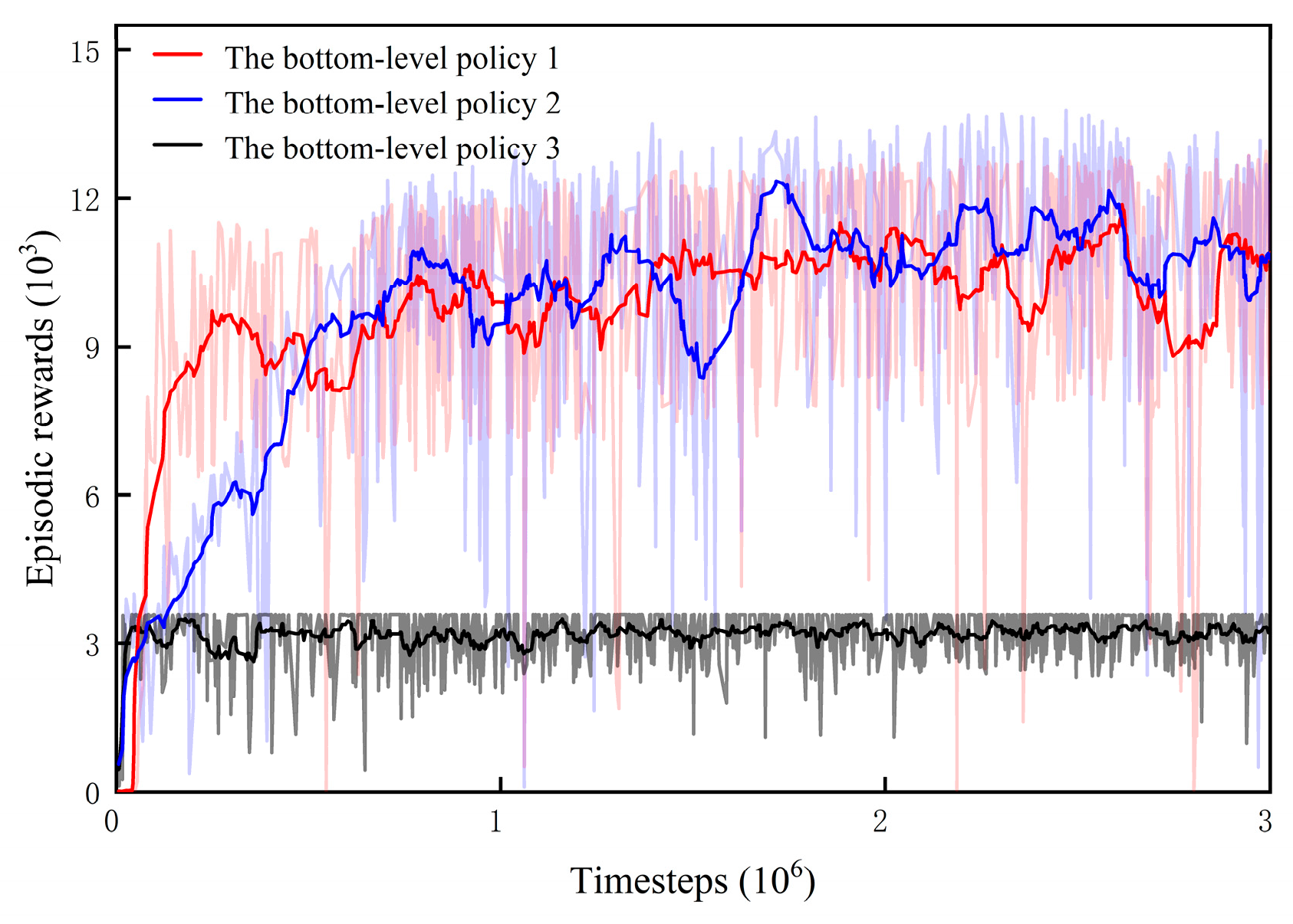
6.2.1. Training and Testing of the Bottom-Level Policies

Figure 12 shows the reward curves during the training process for the bottom-level policies corresponding to Operating Conditions 1, 2, and 3. They have been smoothed using a moving average method with a window size of 50. The horizontal axis represents the number of training steps, and the vertical axis represents the cumulative reward per training episode. After 2.5 million training steps, the episodic rewards for all three bottom-level policies demonstrate convergence. For ease of narration, the bottom-level policies for Operating Conditions 1, 2, and 3 will hereafter be referred to as bottom-level policy 1, bottom-level policy 2, and bottom-level policy 3, respectively.

1.

Testing of bottom-level policy 1

The converged bottom-level policy 1 is used to guide the flight of the Λ-shaped solar-powered UAV, with simulation flight settings as referenced in Table 4. The UAV’s wing deflection angle and battery power curves are shown in Figure 13a, and the solar altitude angle curve is presented in Figure 13b. It can be observed that, due to the low solar altitude angle shortly after sunrise, the efficiency of solar energy absorption is low when the wings are not deflected, and the upward deflection would significantly reduce the illuminated area of the wing upper surfaces. Therefore, the UAV chooses to deflect its wings significantly downward to achieve greater solar energy absorption power. As time progresses and the solar altitude angle gradually increases, the UAV’s wing deflection angle gradually transitions to near 0°, and it continues to fly in an approximately flat configuration.

2.

Testing of bottom-level policy 2

In the testing of bottom-level policy 2, random initial times are selected. The altitude and battery power curves for the trajectory planned by this policy for the Λ-shaped solar-powered UAV are shown in Figure 14a,b. Notably, takeoff times of 6:30 and 11:00 are chosen, which were outside the initial time range set during the training period of bottom-level policy 2. Despite this, the UAV was still able to perform climbing flight normally and maintain good battery power, indicating that the policy possesses a certain generalization capability. This provides an ample time window for selection by the top-level policy, meaning it is not necessary to wait until the earliest initial time specified during the policy’s training phase before this policy can be selected.

3.

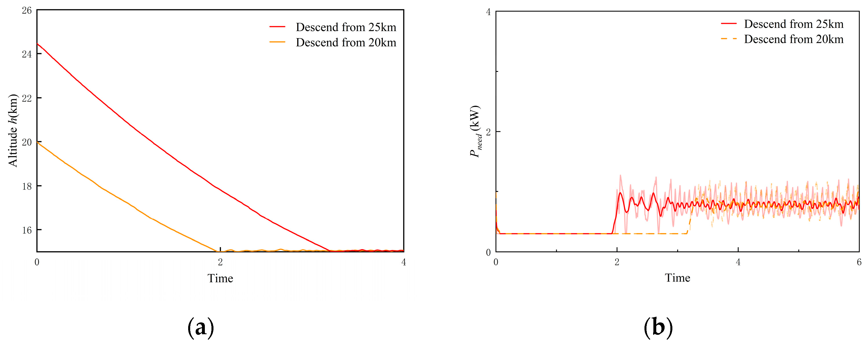
Testing of bottom-level policy 3

In the testing of bottom-level policy 3, different initial altitudes were set. The altitude and battery power curves of the trajectories planned by this policy for the Λ-shaped solar-powered UAV are shown in Figure 15a and Figure 15b, respectively. UAVs released from different initial altitudes, after undergoing powerless gliding, all maintain cruise flight near the minimum altitude with their required power being essentially consistent, which is about 0.76 kW.

The aforementioned tests demonstrate the feasibility of the bottom-level policies to plan trajectories, which can support the subsequent training of the top-level policy.

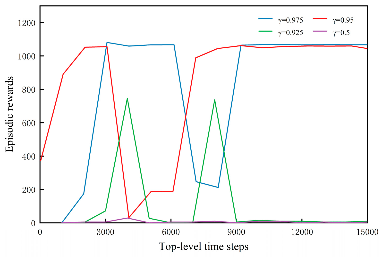
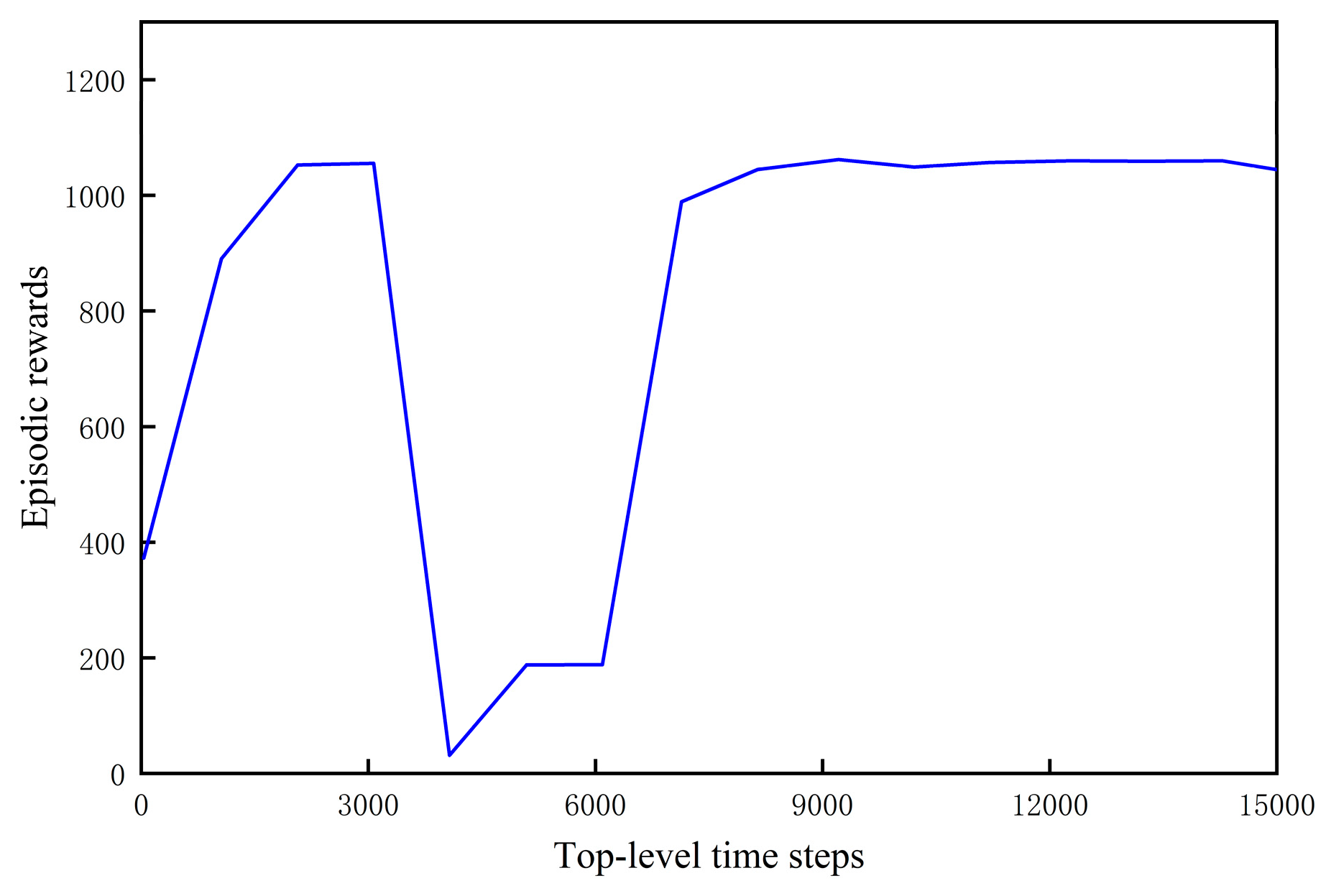
6.2.2. Training of the Top-Level Policy

The reward curve during the training process for the top-level policy is shown in Figure 16. The horizontal axis represents the top-level decision time steps, and the vertical axis represents the cumulative reward per training episode. After 15,000 top-level time steps, which corresponds to 540,000 bottom-level time steps of training, the episodic cumulative reward for the top-level policy demonstrates convergence.

6.2.3. The 24 h Trajectory Simulation and Comparison

As illustrated in Figure 11, the converged bottom-level policies and the top-level policy are combined to form an HRL agent. The agent is used to plan flight trajectories for the Λ-shaped solar-powered UAV on the summer solstice, with relevant settings detailed in Table 7, and the flight duration extended to 24 h. The top-level policy only needs to select between bottom-level policy 1 or 2 during daylight hours; it automatically switches to bottom-level policy 3 when the solar altitude angle falls below $0^{°}$. By setting different random seeds to generate various initial conditions (i.e., initial positions) for the agent’s trajectory planning tasks, the altitude curves and SOC curves of the 24 h trajectories are shown in Figure 17a. It can be seen that the changes in battery energy and gravitational potential energy of the trajectories planned by the agent from any initial condition are consistent. Next, the trajectory based on random seed 156,854 is selected for detailed analysis. This trajectory is plotted as a red curve in Figure 17b. To analyze the optimization performance of the hierarchical policy, the minimum energy consumption State-Machine policy from Section 3.1 is adopted as a comparative baseline. For this State-Machine policy, its high-altitude cruising height is set to be consistent with the minimum high-altitude cruising height of the HRL-planned trajectory. Furthermore, its climb rate during the ascent phase and descent rate during the descent phase are set to the average values observed in the corresponding phases of the HRL-planned trajectory. Other settings remain unchanged, and the trajectory planned by this State-Machine policy is shown as the blue curve in Figure 17b.

The SOC and altitude curves for the Λ-shaped solar-powered UAV in the HRL-planned trajectory are shown in Figure 18a. Throughout the entire process, the altitude comparison curves for the two trajectories are presented in Figure 18b, the energy comparison curves in Figure 18c, and the battery power comparison curves in Figure 19a,b. Comparison curves for state information such as airspeed, thrust, wing deflection angle, bank angle, and attack angle are displayed in Figure 20a–c. The time on the horizontal axis for these figures is converted by setting 4:24 as the zero point. The changing trends of the UAV flight information in both trajectories over the 24 h period are analyzed using the operating condition classification method outlined in Table 2.

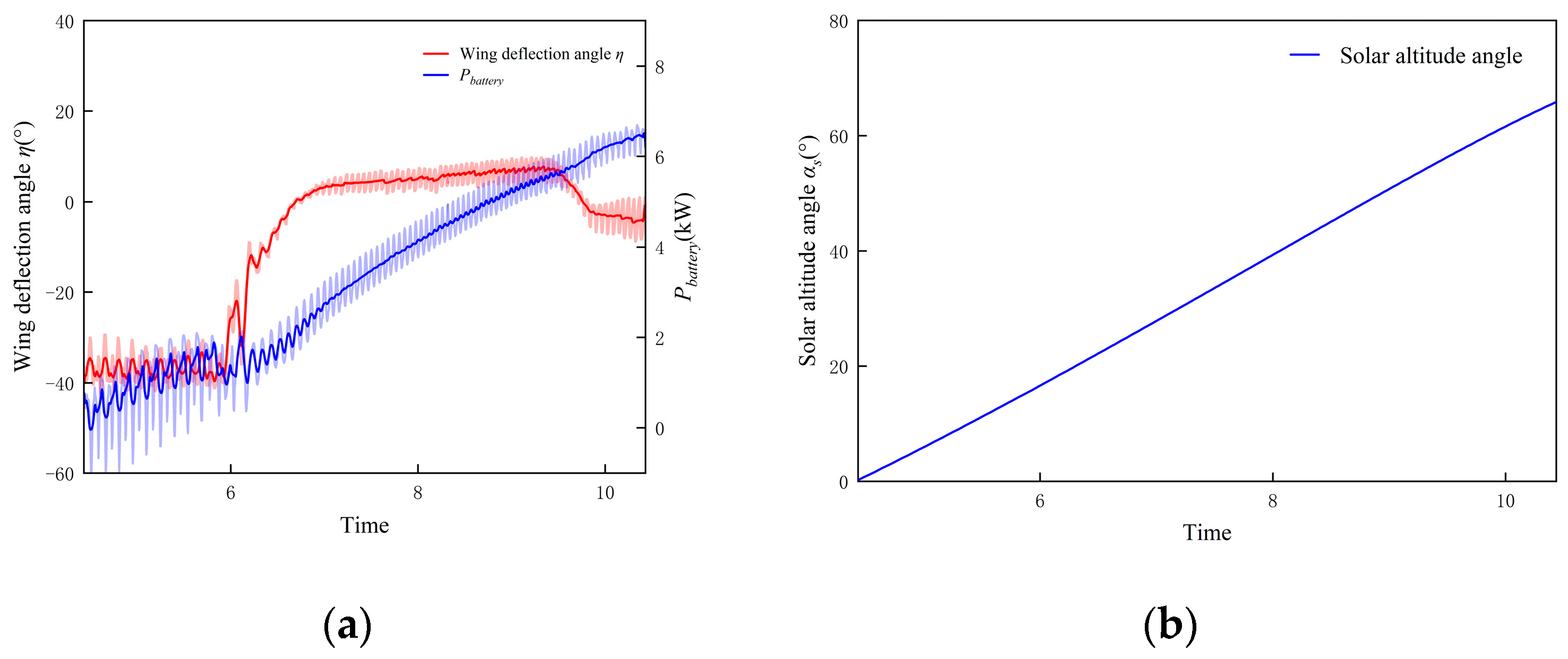
• Operating Condition 1: During daytime with scarce battery energy.

The Λ-shaped solar-powered UAV commences its flight at 4:24 with a SOC of 30%. The top-level policy selects the bottom-level policy 1 to guide the UAV until 8:02, a duration of 3.6 h. During this period, the charging process of the UAV can be divided into two phases: 4:24–6:44 and 6:44–8:02. This aligns with the test results shown in Figure 13. In the first phase, the UAV maintains a wing deflection angle of approximately −40° to achieve a more optimal solar incidence angle. In the subsequent phase, as the solar altitude angle gradually increases, the UAV’s wings tend to flatten. In contrast, the UAV with the State-Machine policy consistently maintains a wing deflection angle of 9.26° to preserve optimal lift coefficient. As illustrated in Figure 19a and Figure 20b,c, during the 4:24–6:44 interval, compared to the State-Machine policy, the hierarchical policy results in the UAV’s airspeed being approximately 5 m/s higher and its thrust approximately 10 N higher, which increases the required power. However, while ensuring an effective illuminated area, it significantly enhances the UAV’s solar energy absorption efficiency. The maximum difference in battery power between the two policies can reach up to 2.36 kW. Between 6:44 and 8:02, even after the wings tend to flatten, the hierarchical policy can still shorten the battery power fluctuation period by employing a smaller turning radius. Concurrently, as indicated by Figure 18b and Figure 19b, during this time, the UAV following the hierarchical policy gradually increases its altitude to 16 km to pursue greater solar irradiation intensity. The gain in solar energy absorption power resulting from this operation is sufficient to compensate for the additionally incurred required power, thereby allowing its battery power to remain higher than that of the State-Machine policy. During Operating Condition 1, the thrust of the UAV guided by the hierarchical policy is maintained at approximately 26 N, slightly higher than the 22 N of the State-Machine policy, while its SOC growth rate is significantly higher than the latter, as can be clearly observed in Figure 18c.

2.

Operating Condition 2: During daytime with abundant battery energy.

The top-level policy selected the bottom-level policy 2 starting from 8:02 and continued to do so until sunset. As can be seen in Figure 18a, when the UAV begins its climb guided by the bottom-level policy 2, its SOC is approximately 78%. This is because the reward function used during the training of the top-level policy incorporates both battery energy and gravitational potential energy. Initiating the climb from 8:02 has a relatively minor impact on the SOC growth rate, and instead, it allows for the acquisition of higher total stored energy, comprising both battery energy and gravitational potential energy, for the UAV as a reward. The hierarchical policy guides the UAV to climb from 8:02 to 10:48. The UAV’s thrust first increases to around 75 N, then begins decreasing gradually near 23 km. Upon reaching approximately 24.5 km, it commences high-altitude cruising to avoid exceeding the maximum altitude limit, with the thrust stabilizing at around 24 N. During the climb, the UAV’s airspeed gradually increases to around 32 m/s, while the absolute value of the wing deflection angle decreases, and the attack angle simultaneously increases to obtain higher aerodynamic lift. After entering high-altitude cruising, the UAV’s wing deflection angle, attack angle, and roll angle stabilize around 0°, 4°, and 3°, respectively. Compared to the cruise phase between 6:44 and 8:02 at an altitude of approximately 16 km, which is characterized by low wing deflection angles, both the attack angle and roll angle are slightly elevated. Driven by bottom-level policy 2, as the Λ-shaped UAV cruises at high altitude and approaches evening, it will re-deflect its wings to maintain a battery power greater than zero. It is not until 18:34 that it can no longer sustain a full charge. After 18:53, the UAV will reduce its cruise altitude to lower its required power, continuing until it enters the nighttime phase at 19:15.

As can be seen from Figure 18b,c and Figure 20b,c, the UAV with the State-Machine policy only initiates its climb after its SOC reaches the threshold, which is 95%, and its thrust and airspeed during climbing are lower than those of the UAV with the hierarchical policy. Consequently, it reaches full charge earlier than the UAV guided by the hierarchical policy, which starts climbing sooner. However, the UAV with the hierarchical policy benefits from its superior charging efficiency during Operating Condition 1, meaning its time to reach full charge is only 0.19 h later. Furthermore, the hierarchical policy’s decision to climb earlier enables its UAV to enter the full-charge high-altitude cruising stage 0.4 h sooner than the UAV with the State-Machine policy. From Figure 20a, during high-altitude cruising, the UAV with the State-Machine policy maintains its wing deflection at an approximately flat state of −0.89° to achieve maximum aerodynamic lift. However, this also reduces its solar energy absorption efficiency. As a result, it is unable to maintain a 100% SOC while cruising at high altitude after 17:59, and begins to descend according to the rules, which is 0.58 h earlier than the hierarchical policy. Therefore, throughout the entire full-charge high-altitude cruising stage, the UAV with the hierarchical policy cruises for 0.98 h longer than the one with the State-Machine policy.

3.

Operating Condition 3: During nighttime.

The UAV with the State-Machine policy starts unpowered descent at 17:59, whereas the hierarchical policy switches to the bottom-level policy 3 at 19:15 to initiate unpowered descent. At the same descent rate, the bottom-level policy 3 enables the UAV to maintain zero thrust throughout the descent, while the duration for which the State-Machine policy maintains zero thrust is slightly shorter. Because the State-Machine policy initiates unpowered descent as soon as the battery power drops below zero, its SOC can remain at 100% until 19:15. In contrast, when the hierarchical policy initiates unpowered descent at 19:15, its SOC is already below 100%. Consequently, at the beginning of Operating Condition 3, the battery energy of the UAV with the State-Machine policy is superior to that of the UAV with the hierarchical policy, as shown in Figure 18c. However, this also leads to the State-Machine policy starting low-altitude cruising approximately 1.2 h earlier than the hierarchical policy, which results in higher battery energy consumption. During the descent stage, the airspeed, bank angle, and attack angle of the UAVs in both trajectories gradually decrease, while their wings are deflected to some extent within the −20° to 30° range to adjust aerodynamic efficiency. After entering low-altitude cruising, from Figure 19a and Figure 20a–c, the UAV with the State-Machine policy maintains a wing deflection angle of 9.26° and flies at a minimum airspeed of 15 m/s. In contrast, the UAV with the hierarchical policy, to avoid falling below the minimum airspeed limit, maintains its airspeed around 16 m/s. Its wing deflection angle fluctuates between 0° and 15° with circling flight, and its average battery power is only about 0.0269 kW lower than that of the State-Machine policy.

4.

Evaluation of the necessity of the top-level policy

The analysis of Operating Condition 2 mentions that the UAV with the hierarchical policy starts climbing when the SOC is approximately 78%, which originates from the decision of the top-level policy. The previous comparison has proven the superiority of the bottom-level policies, and the necessity of the top-level policy’s long-term planning capability for the hierarchical agent also needs to be evaluated. A new comparative case is set up as a flat agent that removes the top-level policy and retains only the bottom-level policies, which are switched by a rule. The rule follows the State-Machine policy, first executing the bottom-level policy 1, and switching to the bottom-level policy 2 after the SOC reaches the threshold of 95%. With the random seed and other conditions unchanged, the altitude and energy curves of the trajectories planned by the hierarchical agent and the flat agent are compared, as shown in Figure 21. It can be seen that the final remaining battery energy and total remaining energy of the rule-driven flat agent are consistent with those of the hierarchical agent, as both adopt the same bottom-level policies. However, while the hierarchical agent takes 0.28 h longer to fully charge compared to the flat agent, it can start climbing approximately 0.6 h earlier and has a better total energy storage status. This result indicates that the top-level policy in the hierarchical agent is necessary for the UAV to maintain optimal total energy stored during the 24 h flight period.

Through the aforementioned comparative simulations and analysis, the HRL-based trajectory planning policy for the Λ-shaped solar-powered UAV demonstrates two key advantages in terms of energy optimization.

(1)

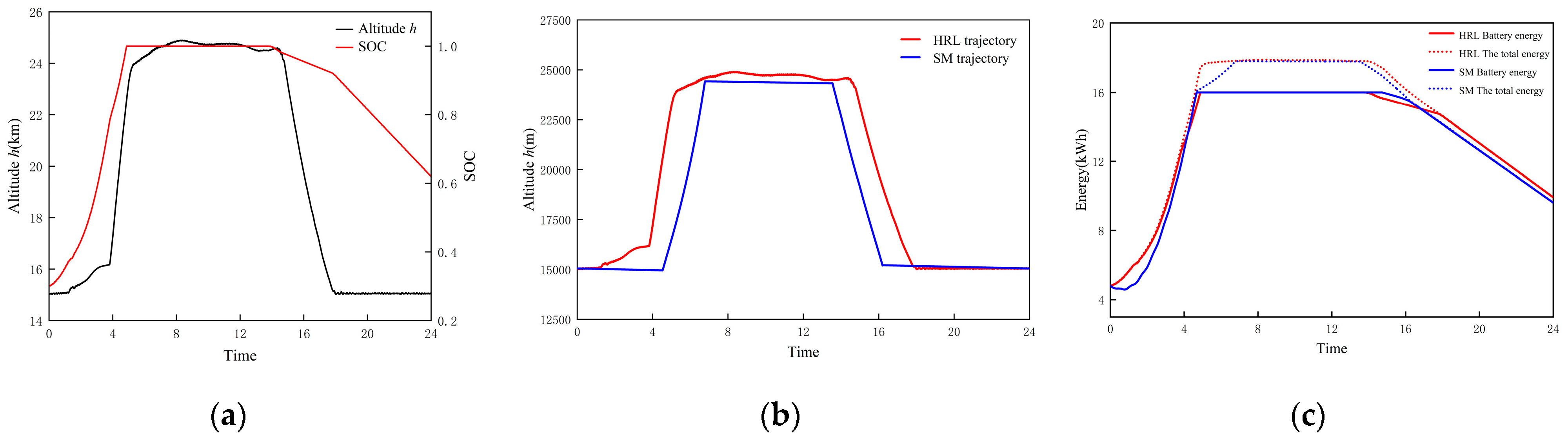
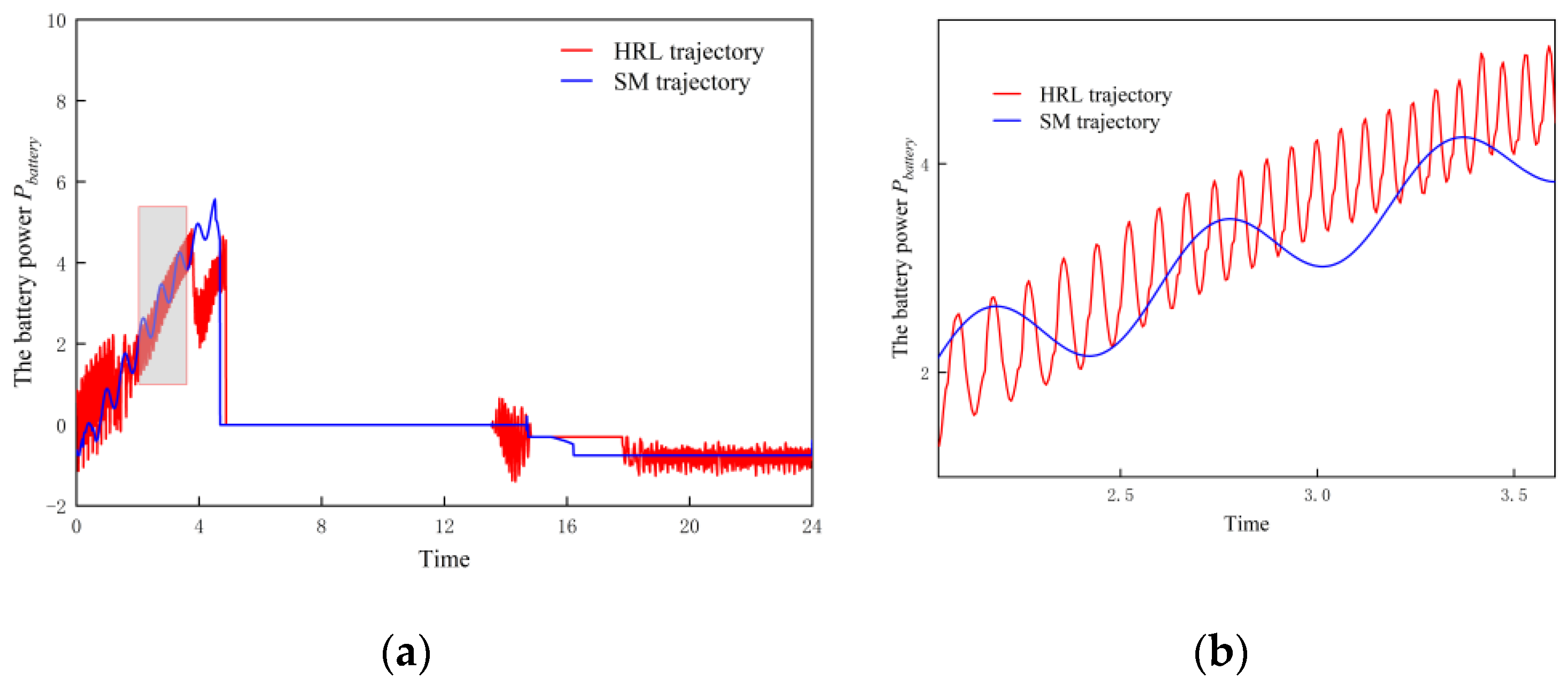
Superior energy state during flight: This policy enables the UAV to achieve better solar energy absorption efficiency during the charging stage, allowing its SOC to continuously increase. In contrast, the battery energy of the UAV with the State-Machine policy experiences a brief decrease after takeoff. Regarding gravitational potential energy storage, this policy does not adhere to the traditional heuristic of climbing only after reaching full charge. Instead, it makes autonomous decisions based on its own energy status and environmental energy information. By starting to climb earlier, it achieves a longer duration of optimal total energy stored, and the comparison with the flat agent strongly corroborates this result. The superior solar energy absorption capability of this policy’s bottom-level sub-policy as sunset approaches further extends this period. This is specifically manifested as an additional 0.98 h of full-charge high-altitude cruising duration compared to the State-Machine policy.

(2)

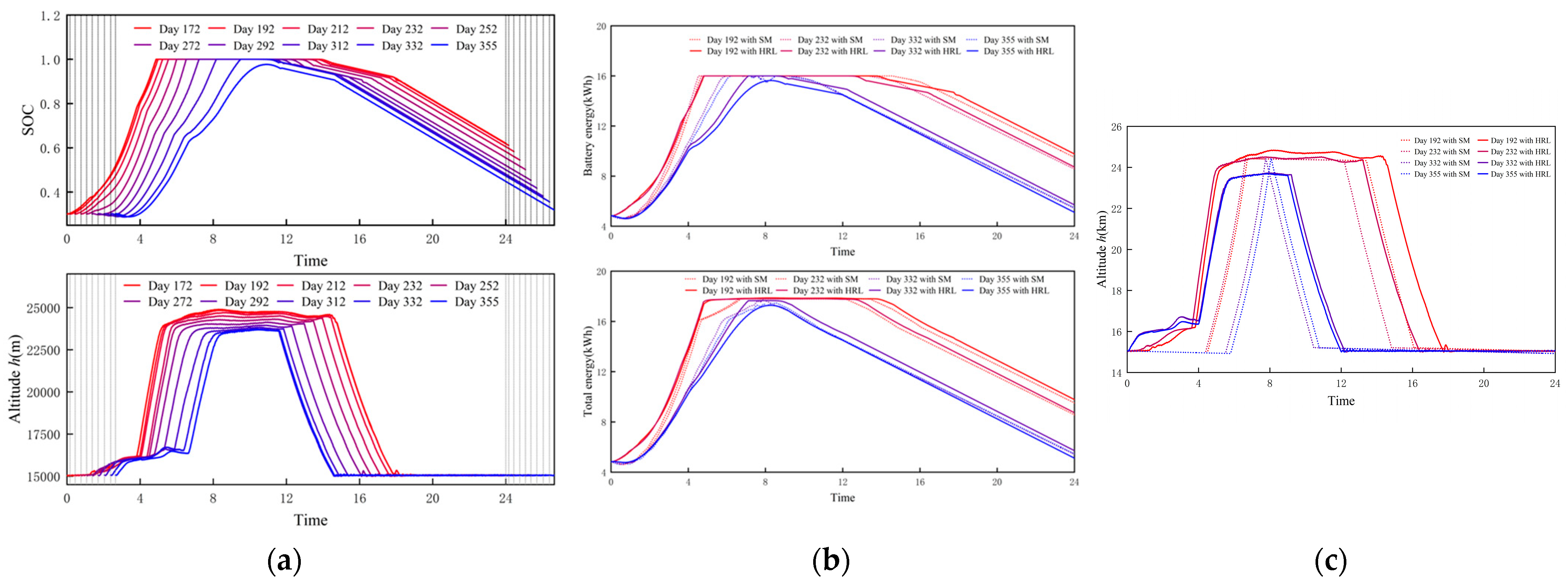
More remaining energy: The remaining energy of the UAV after a 24 h flight is the most direct indicator for evaluating its energy-optimal trajectory planning policy. After completing the 24 h flight, the UAV guided by this policy has a remaining battery energy of 9.93 kWh, a remaining total stored energy of 9.94 kWh, and a remaining SOC of 62.04%. The UAV guided by the State-Machine policy has a remaining battery energy of 9.62 kWh, a remaining total stored energy of 9.63 kWh, and a remaining SOC of 60.12%. Compared to the latter, the former results in 0.31 kWh more remaining battery energy, 0.31 kWh more remaining total stored energy, and 1.92% higher remaining SOC, thus achieving better energy returns.

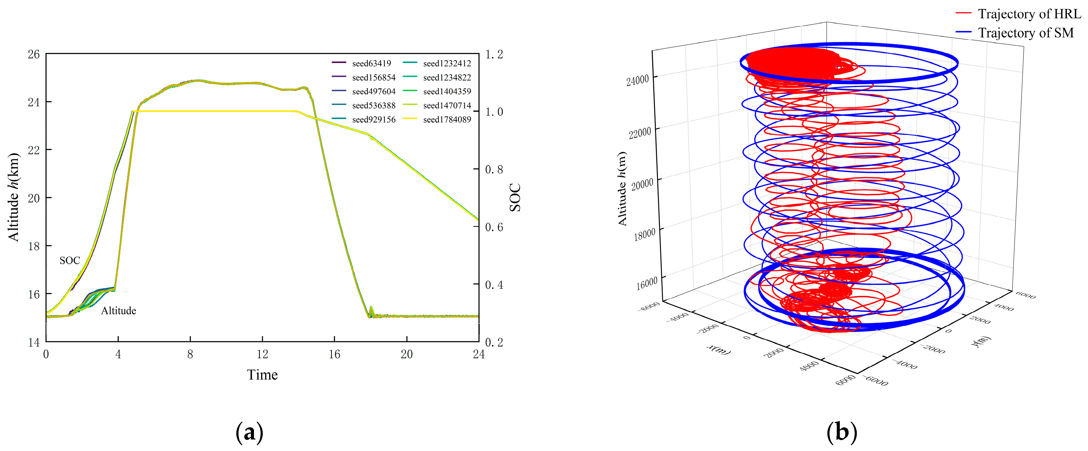
6.2.4. Testing of the Generalization Ability

To test the generalization ability of the hierarchical planning policy, one day is selected every 20 days from the summer solstice to the winter solstice for the Λ-shaped UAV to conduct simulated flights guided by the hierarchical agent. Except for adjusting the initial time to the sunrise time of the day, all other settings remained unchanged. The obtained flight profiles are shown in Figure 22a, where the zero point on the horizontal axis represents the real time of 4:24, indicating that the hierarchical agent trained based on the summer solstice can still generate effective trajectories on other dates. The SOC curves show that the 24 h remaining battery energy of the UAV gradually decreases from the summer solstice to the winter solstice, as the sunrise time is continuously delayed and the sunset time is continuously advanced, causing a gradual extension of nighttime. According to the altitude curves, the hierarchical agent can adapt to changes in flight dates, gradually delaying the climbing time and reducing the height of high-altitude cruising to effectively pursue the total energy. The test results on days 192, 232, 332, and 355 (i.e., the winter solstice) are selected for comparison with the State-Machine policy, as shown in Figure 22b,c. It can be seen that until day 332, the hierarchical agent still has advantages in the UAV’s remaining energy, high-altitude cruising duration, and total energy storage status, proving that the HRL-based trajectory planning policy has powerful cross-quarter adaptive capability. It is worth noting that the reason why the hierarchical policy shows disadvantages on the winter solstice is that it fails to postpone the climbing time in a more timely manner, resulting in an excessive decrease in the SOC growth rate caused by climbing. The UAV fails to fully charge during the daytime, and the obtained gravitational potential energy cannot make up for the indirect loss of battery energy caused by the decision. This indicates that the winter solstice environment exceeds the adaptation range of the hierarchical policy based on the summer solstice.

7. Conclusions and Future Work

This paper proposes a trajectory planning policy based on HRL to address the 24 h energy-optimal trajectory planning problem for a Λ-shaped morphing solar-powered UAV. First, a detailed mathematical simulation model was established, encompassing aerodynamics, energy, and dynamics and kinematics. Secondly, based on the variations of the UAV’s self-energy and environmental energy along a minimum energy consumption benchmark trajectory, a flight operating condition classification method was proposed, and corresponding optimization focuses were identified for different operating conditions. Thirdly, according to the operating condition classification results, an HRL method based on the Options Framework was adopted, combining the DQN and SAC algorithms, to design the training method for the hierarchical trajectory planning policy of the Λ-shaped solar-powered UAV. Finally, simulation results indicate that after training convergence, the bottom-level policies of the hierarchical policy can output appropriate commands for thrust, attitude angles, and wing deflection angles, to pursue their respective optimization objectives. Meanwhile, the top-level policy of the hierarchical policy can appropriately switch between bottom-level policies based on flight information during daytime flight to achieve a better self-energy state. Comparison with the minimum energy consumption benchmark trajectory shows that the HRL-based trajectory planning policy can effectively increase the UAV’s full-charge high-altitude cruising duration and its remaining self-energy after a 24 h flight. The testing of generalization ability proves that the hierarchical policy can also autonomously adapt to new dates with intervals of several months. Therefore, this method not only ensures real-time and autonomous trajectory planning but also demonstrates excellent energy optimization capability and environmental adaptability.

The future work is expected to focus on the following three aspects. Firstly, in terms of model improvement, the influence of wind fields will be further considered in the environmental model. Although the wind field gradient in the stratosphere is small, the energy provided by the gradient wind field is still a considerable source due to the long flight time of solar UAVs. The research focus will be on balancing the comprehensive effects of wing deflection on wind gradient energy collection, solar energy absorption, and aerodynamic losses. Additionally, the idealized inner-loop response model in this study will be further explored, and DRL algorithms gradually applied to attitude control research will be considered to solve the wing deflection control of morphing solar-powered UAVs. The end-to-end problem of integrating trajectory planning and inner loop control can also adopt an HRL architecture. Secondly, in terms of algorithm design, the state and action spaces of the bottom-level policies in this study are relatively large. Although the standard SAC algorithm can achieve the training purpose, it still requires high training costs. Future plans include improving the existing algorithm by using methods such as prioritized experience replay or pre-training the bottom-level network with offline optimal trajectories generated by classical optimal control methods. Furthermore, integrating wind fields into the environmental model will increase energy optimization indicators, increasing the difficulty of designing reward functions and training policies. In the future, multi-objective reinforcement learning algorithms combining reinforcement learning and multi-objective optimization will be considered to improve the hierarchical trajectory planning policy, achieving the best balance among various energy indicators. Thirdly, in terms of practical validation, the trained neural networks will be deployed on embedded flight control computers, and their effectiveness will be validated through hardware-in-the-loop simulations and scaled prototype flights. Challenges such as latency and computational resource constraints in real deployments of policy networks need to be addressed. These research efforts will provide theoretical support and technical reference for enhancing the intelligence, endurance, and mission efficiency of morphing configuration solar-powered UAVs.

References

1. Zhu, X.; Guo, Z.; Hou, Z. Solar-Powered Airplanes: A Historical Perspective and Future Challenges. Prog. Aerosp. Sci. 2014, 71, 36–53. [Google Scholar] [CrossRef]
2. Alvi, O.U.R. Development of Solar Powered Aircraft for Multipurpose Application. In Collection of Technical Papers—AIAA/ASME/ASCE/AHS/ASC Structures, Structural Dynamics and Materials Conference; American Institute of Aeronautics and Astronautics Inc. (AIAA): Reston, VA, USA, 2010. [Google Scholar]
3. Wang, S.Q.; Ma, D.L. Three dimensional trajectory optimization of high-altitude solar powered unmanned aerial vehicles. J. Beijing Univ. Aeronaut. Astronaut. 2019, 45, 936–943. [Google Scholar] [CrossRef]
4. Richfield, P. Aloft for 5 Years: DARPA’s Vulture Project Aims for Ultra Long UAV Missions. Def. News 2007, 22, 30. [Google Scholar]
5. Gao, Z.X. General planning method for energy optimal flight path of solar-powered aircraft in near space. Chin. J. Aeronaut. 2023, 44, 6–27. [Google Scholar]
6. Klesh, A.; Kabamba, P. Energy-Optimal Path Planning for Solar-Powered Aircraft in Level Flight. In Collection of Technical Papers—AIAA Guidance, Navigation, and Control Conference 2007; AIAA: Hilton Head, SC, USA, 2007; Volume 3, pp. 2966–2982. [Google Scholar] [CrossRef]
7. Spangelo, S.C.; Gilbert, E.G. Power Optimization of Solar-Powered Aircraft with Specified Closed Ground Tracks. J. Aircr. 2013, 50, 232–238. [Google Scholar] [CrossRef]
8. Huang, Y.; Chen, J.; Wang, H.; Su, G. A Method of 3D Path Planning for Solar-Powered UAV with Fixed Target and Solar Tracking. Aerosp. Sci. Technol. 2019, 92, 831–838. [Google Scholar] [CrossRef]
9. Ailon, A. A Path Planning Approach for Unmanned Solar-Powered Aerial Vehicles. Renew. Energy Power Qual. J. 2023, 21, 109–114. [Google Scholar] [CrossRef]
10. Gao, X.-Z.; Hou, Z.-X.; Guo, Z.; Liu, J.-X.; Chen, X.-Q. Energy Management Strategy for Solar-Powered High-Altitude Long-Endurance Aircraft. Energy Convers. Manag. 2013, 70, 20–30. [Google Scholar] [CrossRef]
11. Ma, D.; Bao, W.; Qiao, Y. Study of flight path for solar-powered aircraft based on gravity energy reservation. Hangkong Xuebao/Acta Aeronaut. Astronaut. Sin. 2014, 35, 408–416. [Google Scholar]
12. Marriott, J.; Tezel, B.; Liu, Z.; Stier-Moses, N.E. Trajectory Optimization of Solar-Powered High-Altitude Long Endurance Aircraft. In Proceedings of the 2020 6th International Conference on Control, Automation and Robotics, ICCAR 2020, Singapore, 20–23 April 2020; pp. 473–481. [Google Scholar] [CrossRef]
13. Sun, M.; Shan, C.; Sun, K.-W.; Jia, Y.-H. Energy Management Strategy for High-Altitude Solar Aircraft Based on Multiple Flight Phases. Math. Probl. Eng. 2020, 2020, 6655031. [Google Scholar] [CrossRef]
14. Ni, W.; Ying, B.I.; Di, W.U.; Xiaoping, M.A. Energy-Optimal Trajectory Planning for Solar-Powered Aircraft Using Soft Actor-Critic. Chin. J. Aeronaut. 2022, 35, 337–353. [Google Scholar] [CrossRef]
15. Montalvo, C. Meta Aircraft Flight Dynamics and Controls. Ph.D. thesis, Georgia Institute of Technology, Atlanta, GA, USA, 2014. [Google Scholar]
16. Chao, A.; Xie, C.-C.; Meng, Y.; Liu, D.-X.; Yang, C. Flight dynamics and stable control analyses of multi-body aircraft. Gongcheng Lixue/Eng. Mech. 2021, 38, 248–256. [Google Scholar]
17. Liu, D.; Xie, C.; Hong, G. Dynamic characteristics of wingtip-jointed composite aircraft. J. Beijing Univ. Aeronaut. Astronaut. 2021, 47, 2311–2321. [Google Scholar]
18. Wang, X.; Yang, Y.; Wang, D.; Zhang, Z. Mission-Oriented Cooperative 3D Path Planning for Modular Solar-Powered Aircraft with Energy Optimization. Chin. J. Aeronaut. 2022, 35, 98–109. [Google Scholar] [CrossRef]
19. Wu, M.; Xiao, T.; Ang, H.; Li, H. Optimal Flight Planning for a Z-Shaped Morphing-Wing Solar-Powered Unmanned Aerial Vehicle. J. Guid. Control. Dyn. 2018, 41, 497–505. [Google Scholar] [CrossRef]
20. Wu, M.; Shi, Z.; Ang, H.; Xiao, T. Theoretical Study on Energy Performance of a Stratospheric Solar Aircraft with Optimum Λ-Shaped Rotatable Wing. Aerosp. Sci. Technol. 2020, 98, 105670. [Google Scholar] [CrossRef]
21. Wu, M.; Shi, Z.; Xiao, T.; Ang, H. Flight Trajectory Optimization of Sun-Tracking Solar Aircraft under the Constraint of Mission Region. Chin. J. Aeronaut. 2021, 34, 140–153. [Google Scholar] [CrossRef]
22. Li, Z.-r.; Yang, Y.-p.; Zhang, Z.-j.; Ma, X.-p. Overall Design and Energy Efficiency Optimization for Communication-Oriented Morphing Solar-Powered UAV. J. Beijing Univ. Aeronaut. Astronaut. 2022, 48. [Google Scholar] [CrossRef]
23. Ma, D.; Bao, W.; Qiao, Y. Study of solar-powered aircraft configuration beneficial to winter flight. Hangkong Xuebao/Acta Aeronaut. Et Astronaut. Sin. 2014, 35, 1581–1591. [Google Scholar]
24. Wang, S.; Ma, D.; Yang, M.; Zhang, L.; Li, G. Flight Strategy Optimization for High-Altitude Long-Endurance Solar-Powered Aircraft Based on Gauss Pseudo-Spectral Method. Chin. J. Aeronaut. 2019, 32, 2286–2298. [Google Scholar] [CrossRef]
25. Martin, R.A.; Gates, N.S.; Ning, A.; Hedengren, J.D. Dynamic Optimization of High-Altitude Solar Aircraft Trajectories under Station-Keeping Constraints. J. Guid. Control. Dyn. 2019, 42, 538–552. [Google Scholar] [CrossRef]
26. Pandian, A.P.D. Sustainable Energy Efficient Unmanned Aerial Vehicles with Deep Q-Network and Deep Deterministic Policy Gradient. In Proceedings of the 2024 International Symposium on Networks, Computers and Communications, ISNCC 2024, Washington, DC, USA, 22–25 October 2024. [Google Scholar] [CrossRef]
27. Chen, S.; Mo, Y.; Wu, X.; Xiao, J.; Liu, Q. Reinforcement Learning-Based Energy-Saving Path Planning for UAVs in Turbulent Wind. Electronics 2024, 13, 3190. [Google Scholar] [CrossRef]
28. Li, Y.; Aghvami, A.H.; Dong, D. Path Planning for Cellular-Connected UAV: A DRL Solution With Quantum-Inspired Experience Replay. IEEE Trans. Wirel. Commun. 2022, 21, 7897–7912. [Google Scholar] [CrossRef]
29. Reddy, G.; Wong-Ng, J.; Celani, A.; Sejnowski, T.J.; Vergassola, M. Glider Soaring via Reinforcement Learning in the Field. Nature 2018, 562, 236–239. [Google Scholar] [CrossRef]
30. Xi, Z.; Wu, D.; Ni, W.; Ma, X. Energy-Optimized Trajectory Planning for Solar-Powered Aircraft in a Wind Field Using Reinforcement Learning. IEEE Access 2022, 10, 87715–87732. [Google Scholar] [CrossRef]
31. Sutton, R.S.; Precup, D.; Singh, S. Between MDPs and Semi-MDPs: A Framework for Temporal Abstraction in Reinforcement Learning. Artif. Intell. 1999, 112, 181–211. [Google Scholar] [CrossRef]
32. Chai, J.; Chen, W.; Zhu, Y.; Yao, Z.-X.; Zhao, D. A Hierarchical Deep Reinforcement Learning Framework for 6-DOF UCAV Air-to-Air Combat. IEEE Trans. Syst. Man Cybern.-Syst. 2023, 53, 5417–5429. [Google Scholar] [CrossRef]
33. Lv, C.; Zhu, M.; Guo, X.; Ou, J.; Lou, W. Hierarchical Reinforcement Learning Method for Long-Horizon Path Planning of Stratospheric Airship. Aerosp. Sci. Technol. 2025, 160, 110075. [Google Scholar] [CrossRef]
34. Raoufi, M.; Telikani, A.; Zhang, T.; Shen, J. Fire Front Path Planning and Tracking Control of Uncrewed Aerial Vehicles Using Deep Reinforcement Learning. Robot. Auton. Syst. 2025, 193, 105076. [Google Scholar] [CrossRef]
35. Kong, W.; Zhou, D.-Y.; Du, Y.-J.; Zhou, Y.; Zhao, Y.-Y. Hierarchical Multi-Agent Reinforcement Learning for Multi-Aircraft Close-Range Air Combat. IET Control Theory Appl. 2023, 17, 1840–1862. [Google Scholar] [CrossRef]
36. Wang, H.T.; Yu, C.M. Trajectory Planning of Morphing Aircraft Based on the Probability of Passing through Threat Zones. Aerosp. Control 2024, 42, 35–41. [Google Scholar] [CrossRef]
37. Sachs, G.; Holzapfel, F. Flight Mechanic and Aerodynamic Aspects of Extremely Large Dihedral in Birds. In Collection of Technical Papers—45th AIAA Aerospace Sciences Meeting, Reno, NV, USA, 8–11 January 2007; AIAA: Reston, VA, USA, 2007. [Google Scholar] [CrossRef]
38. Zhang, J.; Si, J. Study on the Wingbody Longitudinal Characters with Different Wing Dihedral Angles. Chin. J. Appl. Mech. 2013, 30, 167–172. [Google Scholar] [CrossRef]
39. Etkin, B. Dynamics of Atmospheric Flight; Courier Corporation: Chelmsford, MA, USA, 2012. [Google Scholar]
40. Keidel, B. Design and Simulation of High-Flying Permanently Stationary Solar Drones. Ph.D. Dissertation, Technical University of Munich Faculty of Mechanical Engineering, Munich, Bavaria, Germany, 2000. [Google Scholar]
41. Asselin, M. An Introduction to Aircraft Performance; AIAA: Reston, VA, USA, 1997. [Google Scholar]
42. Shiau, J.-K.; Ma, D.-M.; Yang, P.-Y.; Wang, G.-F.; Gong, J.H. Design of a Solar Power Management System for an Experimental UAV. IEEE Trans. Aerosp. Electron. Syst. 2009, 45, 1350–1360. [Google Scholar] [CrossRef]
43. Haarnoja, T.; Zhou, A.; Hartikainen, K.; Tucker, G.; Ha, S.; Tan, J.; Kumar, V.; Zhu, H.; Gupta, A.; Abbeel, P.; et al. Soft Actor-Critic Algorithms and Applications. arXiv 2018, arXiv:1812.05905. [Google Scholar]
44. Guo, S.; Zhao, X. Multi-agent deep reinforcement learning based transmission latency minimization for delay-sensitive cognitive satellite UAV networks. IEEE Trans. Commun. 2022, 71, 131–144. [Google Scholar] [CrossRef]
Figure 1. Schematic diagram of the Ʌ-shaped solar-powered UAV.
Drones 09 00498 g001
Figure 2. (a) Relationship between C L and α, η. (b) Relationship between C D and α, η.
Drones 09 00498 g002
Figure 3. (a) The relationship between C L and η at different α. (b) The relationship between C D and η at different α. (c) The relationship between C L / C D and η at different α.
Drones 09 00498 g003
Figure 4. Aircraft coordinate system and forces.
Drones 09 00498 g004
Figure 5. Angular relationship between photovoltaic cells and solar radiation.
Drones 09 00498 g005
Figure 6. (a) Wing deflection angle η ≤ 0 and the left wing facing away from solar radiation. (b) Wing deflection angle η ≤ 0 and both wings facing solar radiation.
Drones 09 00498 g006
Figure 7. (a) Wing deflection angle η > 0, t a n ( ψ s ) = 0, and there is no oblique illumination in the shaded area of the left wing. (b) Wing deflection angle η > 0, t a n ( ψ s ) > 0, and the length of oblique illumination in the shadow of the left wing does not exceed the chord length. (c) Wing deflection angle η > 0, t a n ( ψ s ) > 0, and the length of oblique illumination in the shadow of the left wing exceeds the chord length.
Drones 09 00498 g007
Figure 8. 24 h minimum energy consumption State-Machine benchmark trajectory.
Drones 09 00498 g008
Figure 9. The total energy state variation curve.
Drones 09 00498 g009
Figure 10. State trajectories of MDP and SMDP.
Drones 09 00498 g010
Figure 11. The hierarchical trajectory planning model for the Ʌ-shaped solar-powered UAV.
Drones 09 00498 g011
Figure 12. Reward curves during bottom-level policy training.
Drones 09 00498 g012
Figure 13. (a) Wing deflection angle and battery power curves for the test cases; (b) Solar altitude angle curve for the test case.
Drones 09 00498 g013
Figure 14. (a) Altitude curves for test cases; (b) Battery power curves for test cases.
Drones 09 00498 g014
Figure 15. (a) Altitude curves for test cases; (b) Required power curves for test cases.
Drones 09 00498 g015
Figure 16. The reward curve during the top-level policy training.
Drones 09 00498 g016
Figure 17. (a) SOC curves and altitude curves of HRL-planned trajectories with different random seeds; (b) 3D trajectories planned by the hierarchical policy (random seed 156,854) and the State-Machine policy.
Drones 09 00498 g017
Figure 18. (a) The SOC and altitude curves in the HRL-planned trajectory; (b) The altitude comparison curves; (c) The energy comparison curves.
Drones 09 00498 g018
Figure 19. (a) The battery power comparison curves; (b) The enlarged section of the battery power curves.
Drones 09 00498 g019
Figure 20. (a) The bank angle and wing deflection angle curves; (b) The attack angle and airspeed curves; (c) The thrust curves.
Drones 09 00498 g020
Figure 21. Comparison between the hierarchical agent and flat agent.
Drones 09 00498 g021
Figure 22. (a) SOC and altitude curves; (b) Battery energy and total energy curves; (c) Altitude curves.
Drones 09 00498 g022