Multi-Layer Path Planning for Complete Structural Inspection Using UAV ^†

Highlights

What are the main findings?

• The proposed algorithm can generate suitable inspection paths for different inspection purposes (distances), including crack detection and photogrammetry.
• The proposed optimization method generates a feasible inspection path that shows improvement in terms of overall turning angle and acceleration when compared with conventional approaches.

What is the implication of the main finding?

• A mixed-viewpoint generation technique is essential in generating suitable inspection path for different purposes while satisfying the varying coverage requirements.
• The inclusion of turning angle in the optimization objective can help improving the overall smoothness of the inspection path, reducing the traversal difficulty.

Abstract

This article addresses the path planning problem for complete structural inspection using an unmanned aerial vehicle (UAV). The proposed method emphasizes the scalability of the viewpoints and aims to provide practical solutions to different inspection distance requirements, eliminating the need for extra view-planning procedures. First, the mixed-viewpoint generation is proposed. Then, the Multi-Layered Angle-Distance Traveling Salesman Problem (ML-ADTSP) is solved, which aims to reduce overall energy consumption and inspection path complexity. A two-step Genetic Algorithm (GA) is used to solve the combinatorial optimization problem. The performance of different crossover functions is also discussed. By solving the ML-ADTSP, the simulation results demonstrate that the mean accelerations of the UAV throughout the inspection path are flattened significantly, improving the overall path smoothness and reducing traversal difficulty. With minor low-level optimization, the proposed framework can be applied to inspect different structures.

1. Introduction

Unmanned aerial vehicles (UAVs) have gained traction across various industries due to their low cost and three-dimensional mobility. Their high mobility and ease of deployment make UAVs suitable for numerous applications, including mapping, reconnaissance, and search and rescue. This paper focuses on one such application: structural inspection.

Current manual inspection techniques are time-consuming and cost-ineffective, prompting many contractors to adopt UAV-aided inspection methods. However, most of these methods still require trained professionals to remotely control the vehicles, which increases operating costs and the risk of human error. An ideal solution is a sensor-equipped UAV that can autonomously navigate around the target structure, minimizing the need for human input. Therefore, a fully autonomous inspection system represents the optimal approach.

For an autonomous inspection system, the coverage path planning problem (CPP) needs to be addressed. This can be divided into two sub-problems: view planning and path generation. The view planning problem, which focuses on data gathering, has been the subject of extensive research. Solutions to this problem can generally be categorized into two types: model-based [1,2,3,4,5,6,7,8,9,10,11,12,13,14,15,16,17,18,19,20,21,22,23] and non-model-based approaches [24,25].

The model-based approach generates viewpoints using a 3D model of the inspection target, while the non-model-based approach, utilizing the “next-best-view” method, generates viewpoints without a 3D model. In this paper, we focus on the model-based approach, which can be further categorized based on its relation to the target’s geometry. Approaches with a closer relation to the inspection target’s geometry typically position viewpoints near the target.

William [1] proposed a model-based view planning approach that generates viewpoints for each surface patch of a rough model of the inspection target. This method formulates and solves a Set Cover Problem (SCP) to obtain the optimal set of viewpoints, followed by solving the Traveling Salesman Problem (TSP) to determine the inspection path connecting all viewpoints. The complexity of this method increases with the refinement level of the 3D model. However, since it was designed for object inspections, such as workpiece quality control, it does not account for inspection path complexity, making it unsuitable for structural inspection. Alexis et al. [2] extended a similar approach to structural inspection. They first generate viewpoints for each triangular mesh of a down-scaled 3D model by offsetting the mesh and then solve the TSP to obtain the inspection path. This method allows for iterative refinement, generating additional viewpoints to cover new meshes, thus offering flexibility for different inspection requirements. Nonetheless, it does not consider path complexity, which increases with model refinement, leading to a sub-optimal inspection path as previous solutions cannot be altered. Brendan and Franz  [3] proposed a sampling-based sweep planning method closely related to the geometry of the inspection target. In this approach, viewpoints are sampled near the selected surface segment, and optimal viewpoints are chosen by solving the SCP. The inspection path is then constructed by connecting these viewpoints through the TSP. This sweep path closely follows the contours of the inspection target, allowing for detailed information gathering with a high-precision sensor. However, this method requires the vehicle to operate very close to the inspection target, necessitating precise maneuvers. Consequently, the high hardware requirements hinder the practical application of this technique.

For view planning approaches that have a lower relation to the geometry of the inspection target, viewpoints are typically located further away from the target. A spherical dilation method was proposed by Tarbox and Gottschlich [4], where viewpoints are generated and sampled on the surface of a sphere that encapsulates the inspection target. While this method achieves a high coverage percentage, it was originally designed for object inspection. When applied directly to structural inspection, the spherical dilation method may lead to significant variations in viewing distance. Additionally, the dilated sphere may encompass nearby structures, potentially causing occlusions that reduce the quality of the gathered information. Jing et al. [5] introduced a sampling-based view planning approach in which viewpoints and their corresponding orientations are sampled within a defined sampling space. The SCP is then solved to obtain the optimal set of viewpoints. This method allows viewpoint generation to be independent of the inspection target’s geometry. However, it relies entirely on sampling, which may prove inadequate if the inspection target is complex or if the sensor specifications are limited.

When designing the inspection path, it is essential to consider the specific inspection techniques being employed. Tarek and Alice [26] summarized various autonomous inspection systems utilized in unmanned aircraft systems (UASs). In brief, the industry primarily employs three main inspection techniques: crack detection [27,28], thermography [29,30], and photogrammetry [31,32]. The inspection distances vary significantly depending on the technique, ranging from 3 meters for crack detection [27] to 25 meters for photogrammetry  [31]. A review of the existing literature indicates that a single viewpoint generation method is insufficient for generating viewpoints with varying distances suitable for different inspection techniques. Since multiple inspection techniques may be required for a single target, a unified viewpoint generation technique is necessary for such applications. The view planning solution should provide a scalable approach that accommodates various inspection purposes.

In this paper, we propose a preliminary path planning framework for comprehensive structural inspection. The framework divides the coverage path planning (CPP) into two subproblems: view planning and path generation. Within the view planning problem, viewpoint generation is categorized into two processes: revolving viewpoints and gap-filling viewpoints. The revolving viewpoints are uniformly distributed around the inspection target, while the gap-filling viewpoints are generated to address any insufficiencies in the revolving viewpoints, ensuring that inspection requirements are met. Unlike other state-of-the-art inspection path planning algorithms, the design of the proposed algorithm considers the requirements of various inspection methods, including viewing distance for close-up inspections and overlapping rate for 3D reconstruction. Consequently, this approach is not limited to a specific inspection method, allowing it to generate suitable inspection paths for diverse inspection applications. A feasible inspection path is generated by solving the Multi-layered Angle-Distance Traveling Salesman Problem (ML-ADTSP), which allows for the creation of a spiral path. The final inspection path can be directly imported into mission planning software and executed using a commercial UAV, such as the DJI Phantom 4 Pro, facilitating the implementation of autonomous inspection. The main contributions of this paper are as follows:

1.

Mixed-viewpoint generation that can generate a scalable viewpoint set that suits different inspection purposes.

2.

A newly proposed ML-ADTSP that can generate a kinodynamically feasible inspection path to ease trajectory optimization in future processes while increasing energy efficiency.

3.

Numerical simulations are performed to extensively study the effects of including kinodynamic constraints during preliminary path planning.

The rest of the paper is organized as follows: Section 2 details the proposed mixed-viewpoint generation framework. Section 3 describes the proposed ML-ADTSP for preliminary path planning. In Section 4, the results of the numerical simulations are provided, and the energy efficiency of the proposed method is proved. Finally, Section 5 concludes the paper.

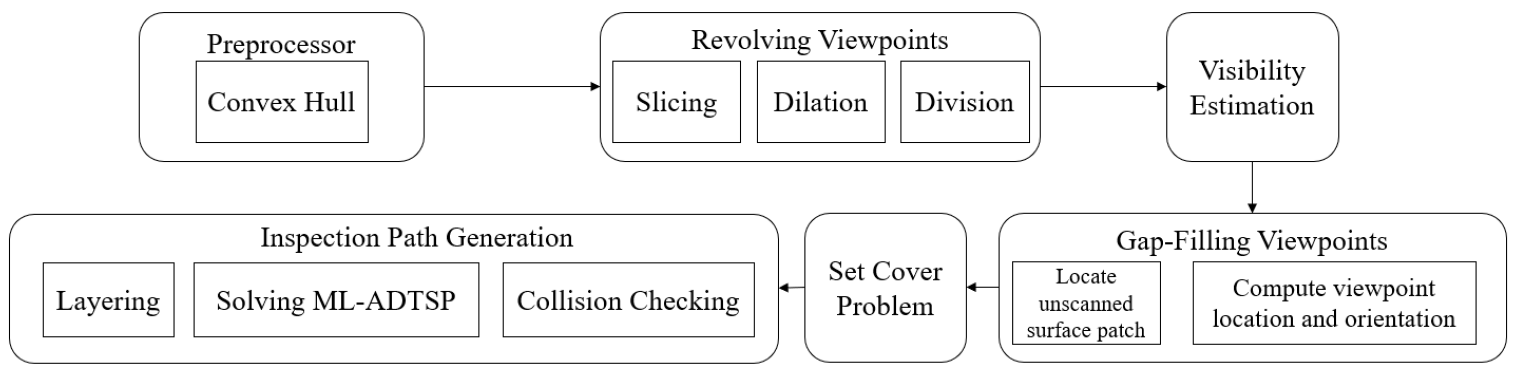
2. Mixed-Viewpoint Generation

The structure of the proposed method is summarized in Figure 1, and it adopted a similar structure as our previous work [33]. A high-definition camera is selected as the sensor, as the information collected can be utilized for both crack detection and photogrammetry. First, the 3D model of the inspection target is processed using a preprocessor to eliminate any convex or concave features. Next, the revolving viewpoints $R_{vp}$ are generated to ensure essential coverage of the inspection target. The visibility information of these viewpoints is evaluated to identify uncovered surface patches. Subsequently, gap-filling viewpoints $G_{vp}$ are explicitly generated to cover these patches. To address significant overlaps among the viewpoints, the SCP is solved to eliminate redundant viewpoints while ensuring that coverage requirements are met. With the optimal set of viewpoints established, the novel ML-ADTSP is solved to obtain a spiral path, enhancing energy efficiency.

To generate a scalable viewpoint set suitable for different inspection purposes, a mixed-viewpoint generation approach is adopted. The revolving viewpoints, which have a higher relation to the target’s geometry, provide guiding points for the inspection path. This ensures that the scalable inspection path maintains consistent viewing distances, thereby enhancing the quality of the data collected. In contrast, the gap-filling viewpoints, which are less dependent on the target’s geometry, offer unique coverage to meet the diverse coverage requirements for various inspection purposes. This combination allows for a comprehensive and adaptable inspection strategy.

2.1. Problem Statement

The proposed inspection path planning algorithm aims to tackle the problem of planning a collision-free inspection that can satisfy the pre-defined inspection requirements. The algorithm assumes that the 3D model of the inspection target is available, and the inspection target is located in an open space such that potential collision with external object and visual occlusions caused by other objects are not considered in this paper.

2.2. Model Preprocessor

In the proposed method, mesh models are utilized instead of point clouds, as they are self-contained and provide additional information, such as surface normals. Consequently, no extra computation is required to acquire the information needed for the path generation process. Furthermore, mesh models can be easily modified using model editing software, such as MeshLab [34].

Before viewpoint generation, the 3D model requires additional refinement. The model may contain convex or concave features, such as balconies, which can increase the risk of intrusion if the UAV closely follows the contours of the inspection target. To minimize these risks, a convex hull is applied to the 3D model, effectively eliminating all concave features. This results in a smooth and featureless model, enhancing the safety and effectiveness of the inspection process.

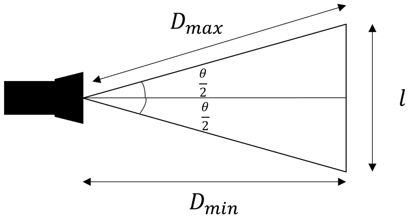
2.3. Revolving Viewpoint Generation

To generate the revolving viewpoint, the contour of the inspection target at different levels is first extracted. The featureless model is divided into different layers through a slicing process. For more flexible slicing size adjustment, the slicing interval is determined by the overlapping rate and the viewing plane height, where the overlapping rate can be adjusted. The vertical viewing plane is illustrated in Figure 2. For a camera with a minimum viewing distance $D_{min}$ and a field of view $\theta$, the height of the vertical viewing plane h should be

$$h=2D_{min}tan\left({\displaystyle \frac{\theta }{2}}\right).$$

(1)

If the slicing interval l equals the viewing plane height h, minimum overlapping is achieved. An overlapping rate $\mu$ is added to h such that

$$l={\displaystyle \frac{2}{\mu }}{D}_{min}tan\left({\displaystyle \frac{\theta }{2}}\right),$$

(2)

with maximum overlapping achieved when $\mu =\infty$ and minimum overlapping achieved when $\mu =1$. The density of the slices can be adjusted based on the inspection requirements. The intersections from each slice are then extracted. A 2D convex hull is applied to the intersections to obtain a polygon that encloses all the intersections. The polygon is then dilated by the minimum viewing distance to create the viewpoint base on which the revolving viewpoints will be generated. The dilated distance ensures that the surface patches are within the viewing distance, allowing the UAV to operate at a safe distance. The slicing process is summarized in Algorithm 1.

Algorithm 1 Viewpoint Base Generation

Input: Surface patches of the 3D model $\mathit{N}(x,y,z)$, Camera matrix $\mathit{C}$, Camera minimum viewing distance $D_{\min }$, Overlapping rate $\mu$. Output: Viewpoint base $\mathit{B}$ 1: $\theta \leftarrow$ FOV$\left(\mathit{C}\right)$ 2: $\Delta l\leftarrow$ FindInterval($D_{\min },\mu ,\theta$) 3: $l_1\leftarrow$${\min }_z$($\mathit{N}$) + $\Delta l$ 4: while $l_i$< ${\max }_z$($\mathit{N}$) do 5:     $Int{t}_i$($x,y,z$) ← Intersection($\mathit{N},l_i$) 6:     ${\mathit{B}}_i\leftarrow$ Convexhull($In{t}_i$($x,y,z$)) 7:     ${\mathit{B}}_i\leftarrow$ Dilate($D_{\min }$, ${\mathit{B}}_i$) 8:     $l_{i+1}\leftarrow l_i$ + $\Delta l$ 9: end while 10: return $\mathit{B}$

To maintain flexibility in viewpoint generation, the overlapping rate should also be used to adjust the number of revolving viewpoints at each level. For a vision cone, the viewing width w is given by

$$w=2D_{min}tan\left({\displaystyle \frac{\theta }{2}}\right).$$

(3)

If the perimeter of the viewpoint base ${\mathit{B}}_i$ at level i is L, minimum horizontal overlapping is achieved when the number of viewpoints is

$$n={\displaystyle \frac{L}{w}}.$$

(4)

By substituting w with ${\displaystyle \frac{2}{\mu }}{D}_{min}tan\left({\displaystyle \frac{\theta }{2}}\right)$, we obtain the general form

$$n={\displaystyle \frac{\mu L}{2D_{min}tan\left(\frac{\theta }{2}\right)}}.$$

(5)

From this general form, it can be observed that maximum horizontal overlapping occurs when $\mu =\infty$, while minimum horizontal overlapping occurs when $\mu =1$. Since the revolving viewpoints are generated along the dilated contour at different levels, collision checks become unnecessary, which helps to reduce computational time.

After the generation of the revolving viewpoints, the visibility information is evaluated. A pinhole camera model [35] is used to simulate the performance of a high-definition camera. The characteristics of the camera can be estimated using the camera matrix, which can be expressed as

$$\mathit{C}=\mathit{K}\times [\mathit{R}\mid t],$$

(6)

where $[\mathit{R}\mid t]$ is the camera extrinsic matrix, which represents the camera’s orientation and position in the 3D world. This matrix consists of the rotation matrix $\mathit{R}$ and the translation vector t. The matrix $\mathit{K}$ is the camera intrinsic matrix, representing the camera’s specifications such as focal length and location of the optical center.

The centroid of the corresponding triangular mesh is used to represent the location of the surface patch. By multiplying the centroid’s location by the camera matrix, as expressed in Equation (7), the arbitrary scalar s and the projection of the centroid on the camera image plane, denoted as ${\left[x_{\mathrm{img}}{y}_{\mathrm{img}}\right]}^T\in {\mathbb{R}}^2$ can be obtained using

$$s{\left[x_{\mathrm{img}}{y}_{\mathrm{img}}1\right]}^T=\mathit{K}\times [\mathit{R}\mid t]\times {\left[x_{\mathrm{world}}{y}_{\mathrm{world}}{z}_{\mathrm{world}}1\right]}^T,$$

(7)

and the visibility can be determined.

The sensor dimensions of the camera are considered when determining visibility. For an image plane with dimensions $[X_{\mathrm{sensor}},Y_{\mathrm{sensor}}]$, if the projection of the world point is within the sensor dimensions, such that

$$0\le x_{\mathrm{img}}\le X_{\mathrm{sensor}}\mathrm{and}0\le y_{\mathrm{img}}\le Y_{\mathrm{sensor}},$$

the surface patch will be visible to the camera.

To ensure image quality, the viewing distance is also limited. The viewing distance should be within an admissible range such that the constraint

$$D_{\min }\le D\le D_{\max }$$

is satisfied. Additionally, to further enhance data quality, the viewing angle $\delta$ is constrained, which is the angle between the surface patch’s normal vector $\overrightarrow{{\mathit{n}}_{\mathit{sp}}}$ and the camera’s viewing direction $\overrightarrow{{\mathit{n}}_{\mathit{vp}}}$.

If the surface patch satisfies all these constraints, it will be considered visible to the camera. A visibility matrix $\mathit{M}$ is generated, where ${\mathit{M}}_{\mathit{i}\mathit{j}}=1$ indicates that the surface patch i is visible to the viewpoint j. With $\mathit{M}$, the overall visibility information of the revolving viewpoints is determined.

2.4. Gap-Filling Viewpoint Generation

The evenly distributed revolving viewpoints may not adequately inspect convex or concave features. Therefore, an additional set of viewpoints, known as gap-filling viewpoints, is required to meet the coverage requirements. After evaluating visibility, the unscanned surface patches and their corresponding normal vectors are extracted. The coordinates of these identified surface patches are extended along their normal vectors by the minimum viewing distance. The new sets of coordinates represent the locations of the gap-filling viewpoints, while the opposite vector of the normal vector indicates the viewing direction.

Using the dilation technique, viewpoints are generated for each unscanned surface patch. However, the resulting viewpoint locations may pose collision risks, especially if the dilated surface patch originates from a concave feature. To mitigate this risk, randomness is introduced into the dilation process. The visibility information is then evaluated, and viewpoints that can provide additional coverage while remaining collision-free are retained. Coverage requirements are also considered; for inspection techniques such as photogrammetry, multiple overlaps are necessary to generate an accurate model. Consequently, viewpoints will also be created for surface patches that do not meet the coverage requirements. Gap-filling viewpoints are generated such that the visibility $M_i$ for surface patch i satisfies the coverage requirement $\epsilon$. Algorithm 2 summarizes the gap-filling viewpoint generation process.

Algorithm 2 Gap-Filling Viewpoint Generation

Input: Unscanned surface patches $\mathit{Surf}(x,y,z)$, Surface patches of 3D model $\mathit{N}(x,y,z)$, Minimum viewing distance $D_{min}$, Normal vectors of unscanned surface patches $\overrightarrow{{\mathit{n}}_{\mathit{sp}}}$ Output: Gap-filling viewpoints ${\mathit{G}}_{\mathit{vp}}(x,y,z)$, Viewing direction $\overrightarrow{{\mathit{n}}_{\mathit{vp}}}$ 1: for $s_i\in \mathit{Surf}$ do 2:      while $M_i<\epsilon$ do 3:          while true do 4:             ${G_{vp}}_i\leftarrow$ RandomSampling($D_{min},s_i,\overrightarrow{{{\mathit{n}}_{\mathit{sp}}}_{\mathit{i}}}$) 5:             $\overrightarrow{{{\mathit{n}}_{\mathit{vp}}}_{\mathit{i}}}\leftarrow$ OppoVector($\overrightarrow{{{\mathit{n}}_{\mathit{sp}}}_{\mathit{i}}}$) 6:             if VisEst(${G_{vp}}_i,\overrightarrow{{{\mathit{n}}_{\mathit{vp}}}_{\mathit{i}}},\mathit{N}$) and ColliCheck(${G_{vp}}_i$) then 7:                ${\mathit{G}}_{\mathit{vp}}\leftarrow$ Append(${\mathit{G}}_{\mathit{vp}},{G_{vp}}_i,\overrightarrow{{{\mathit{n}}_{\mathit{vp}}}_{\mathit{i}}}$) 8:                $M_i$ = $M_i$+1 9:                break 10:            end if 11:          end while 12:     end while 13: end for 14: return ${\mathit{G}}_{\mathit{vp}}$,$\overrightarrow{{\mathit{n}}_{\mathit{vp}}}$

2.5. Time Complexity–Viewpoint Generation

For the viewpoint generation process, the most computationally demanding task is visibility estimation, as it requires evaluating all the surface patches of the 3D model to determine their visibility from each viewpoint. Consequently, the time complexity of the visibility estimation process outweighs that of the viewpoint generation itself. The computation time for visibility estimation is proportional to the number of viewpoints and the complexity of the 3D model, represented as $O\left(n_r{N}_N\right)+O\left(n_g{N}_N\right)$, where $n_r$ and $n_g$ denote the number of revolving and gap-filling viewpoints, respectively, and $N_N$ represents the number of surface patches on the 3D model. This time complexity reflects the worst-case scenario in which the algorithm must evaluate all surface patches to determine visibility. In the proposed algorithm, the 3D model is discretized, allowing only a section of the model to be used in the visibility estimation process. This approach helps prevent excessive computation.

2.6. Set Cover Problem

With the coverage requirements satisfied, an optimal set of viewpoints is essential to minimize the total number of viewpoints. The Set Cover Problem (SCP) is solved for this purpose. The SCP aims to minimize the total number of viewpoints used while meeting the coverage requirements. The SCP of n viewpoints with a coverage requirement $\epsilon$ can be expressed as

$$\begin{array}{cc}\hfill \min \sum _{j=1}^n& x_j,\hfill \\ \hfill \mathrm{s}.\mathrm{t}.\mathrm{for}{V}_i\in \mathit{V},& \sum _{j=1}^n{M}_{ij}\ge \epsilon ,\hfill \\ \hfill \mathrm{where}{x}_n& \in 0,1.\hfill \end{array}$$

(8)

The objective function ensures that the minimum number of viewpoints is selected, while the main constraints guarantee that each surface patch $V_i$ is covered at least $\epsilon$ times, satisfying the minimum coverage requirement. The variable $x_j$ is the decision variable, where $x_j=1$ indicates that the corresponding viewpoint is selected, and $x_j=0$ indicates otherwise.

3. Multi-Layered Angle-Distance Traveling Salesman Problem

With the optimal viewpoint set established, a complete path is needed to connect these viewpoints. While most UAV-aided inspection methods obtain the inspection path by solving the Traveling Salesman Problem (TSP) [2,3,10], they often overlook energy consumption and path smoothness.

A novel Multi-Layered Angle-Distance Traveling Salesman Problem (ML-ADTSP) is formulated to provide an energy-efficient inspection path. Studies [36,37,38] have examined the energy consumption model for UAVs and offer references for energy-efficient path generation. These studies reveal that UAV energy consumption is directly proportional to the distance traveled when flying vertically upwards. Therefore, to minimize vertical motion energy consumption, changes in altitude should be avoided, making a continuously ascending inspection path desirable. For horizontal motion, energy spikes occur when the UAV accelerates; thus, continuous horizontal motion is preferred. Sharp turns, which may cause sudden acceleration and deceleration, should also be avoided to reduce traversal difficulty. In summary, a continuous spiral path is ideal for an energy-efficient inspection. The altitude change should be limited, and the path planning algorithm should focus on minimizing the overall path length and turning angles.

The ML-ADTSP is designed to minimize altitude changes and overall turning angles to reduce energy consumption. The ML-ADTSP can be divided into three steps. First, the viewpoints are categorized into different layers based on their altitude, which limits the overall altitude change. While varying altitudes are permitted within each layer, the resulting inspection path will maintain a spiral shape. After segmentation, the Open-Loop Angle-Distance Traveling Salesman Problem (OL-ADTSP) is solved locally within each layer. By dividing the viewpoints into layers, the number of nodes in each OL-ADTSP is reduced, thereby decreasing the computation time. Finally, the OL-ADTSP tours are connected to obtain a continuous spiral inspection path.

3.1. Angle-Distance Traveling Salesman Problem (ADTSP)

The OL-ADTSP is necessary to create connecting nodes for different layers, and it can be divided into two parts. First, the ADTSP is discussed. The ADTSP aims to minimize the total tour length and the total turning angle. The formulations of the problem are as follows:

$$min{w}_1\sum _{i=1}^n\sum _{i\ne j,j=1}^n{d}_{ij}{p}_{ij}+w_2\sum _{i=1}^n\sum _{i\ne j,j=1}^n\sum _{i\ne j\ne k,k=1}^n{a}_{ijk}{q}_{ijk},$$

(9)

$$\mathrm{s}.\mathrm{t}.\sum _{i=1,i\ne j}^n{p}_{ij}=1,\forall j\in V,$$

(10)

$$\sum _{j=1,j\ne i}^n{p}_{ij}=1,\forall i\in V,$$

(11)

$$\sum _{i\ne j\in S}{p}_{ij}\le \left|S\right|-1\forall S\subset V,S\ne \varnothing ,$$

(12)

$$p_{ij}\in 0,1,$$

(13)

$$q_{ijk}\in 0,1.$$

(14)

where $w_1$ and $w_2$ are the weights for the total distance cost $c_d$ and the total turning angle cost $c_a$, respectively. $p_{ij}$ and $q_{ijk}$ are the decision variables, representing the connections between nodes 2 and 3, respectively. The term $d_{ij}$ represents the distance cost of the path $p_{ij}$, which connects nodes i and j. The term $a_{ijk}$ represents the turning angle cost of three consecutive nodes i, j, and k, which can be expressed as

$$a_{ijk}=arccos({\displaystyle \frac{p_j-p_i}{\parallel p_j-p_i\parallel }}·{\displaystyle \frac{p_k-p_j}{\parallel p_k-p_j\parallel }}).$$

(15)

The turning angle considered is the yaw angle of the UAV, which is independent of the camera’s yaw. Constraints (10) and (11) ensure that for each node, there exists one entry path and one exit path. Constraint (12) is the subtour elimination constraint, which ensures that a complete tour can be obtained. Constraints (13) and (14) guarantee the integrality of the variables.

Since the distance cost only considers two consecutive nodes, while the turning angle cost considers three consecutive nodes, different variables are needed to represent them. In addition, separated arrays are required to store the distance and turning angle data as they are computed differently. To ease the computation process, the formulated problem can benefit from the unification of variables. Specifically, the formulations can be further simplified by replacing $p_{ij}$ with $q_{ijk}$ and $d_{ij}$ with $d_{ijk}$, such that the distance cost is associated with every three nodes visited consecutively.

$$\min w_1\sum _{i=1}^n\sum _{i\ne j,j=1}^n\sum _{i\ne j\ne k,k=1}^n{d}_{ijk}{q}_{ijk}+w_2\sum _{i=1}^n\sum _{i\ne j,j=1}^n\sum _{i\ne j\ne k,k=1}^n{a}_{ijk}{q}_{ijk},$$

(16)

$$\mathrm{subject} \mathrm{to}{p}_{ij}=\sum _{(i,j,k)\in V}{q}_{ijk}=\sum _{(k,i,j)\in V}{q}_{kij},(i,j)\in A.$$

(17)

Constraint (17) ensures that for a selected arc $(i,j)\in A$, there exists a node $k\in V$ such that the path $(i,j,k)$ is included in the tour. Additionally, there must exist another node $k^{\prime }\in V$ such that the path $(k^{\prime },i,j)$ is also included in the tour. As proven in [39], this ADTSP model is a formulation of the Quadratic Traveling Salesman Problem (QTSP).

The Genetic Algorithm (GA) [40] is selected to solve the combinatorial optimization problem due to its well-established application to the TSP. The GA offers fast computation times and high flexibility in terms of algorithm design. Its modular genetic operators can be swapped in and out to suit specific optimization objectives. The GA is a search algorithm that aims to discover superior genetic features and improve candidate solutions based on those features. It initially generates a random set of candidate solutions $G_c$, also known as the population. The corresponding fitness values for these solutions are calculated. Elitism is performed to retain candidate solutions with higher fitness values, passing them to the next generation $G_n$. Different evolution functions are then applied to the candidate solutions based on probability. Crossover is performed first, where two parents with high fitness values are selected to produce a child candidate solution. This child solution retains the superior genetic features and may outperform the parents, fulfilling the evolutionary purpose. To prevent the population from getting trapped in local minima, mutation is required. Under this function, some features in the candidate solution are altered. Through these evolution functions, a new population of solutions is generated that is distributed across the search space, leading to improved fitness values. The overall fitness continues to enhance across different generations. The GA searches for the optimal combination in consecutive iterations until the terminating condition is met. The structure of the GA is summarized in Algorithm 3.

Algorithm 3 Genetic Algorithm for ADTSP

Input: Number of generations $N_G$, Population Size $N_p$, Elitism Rate $P_E$, Crossover Rate $P_c$, Mutation Rate $P_M$. Output: Close Loop Tour for the ADTSP T 1: $G_c\leftarrow$ Initialize($N_P$) 2: Fitness value evaluation 3: for $i\leftarrow 2$ to $N_G$ do 4:     $Elite\leftarrow$ Elitism($G_c,P_E$) 5:     $G_n\leftarrow$ Append($Elite,G_n$) 6:     for $j\leftarrow N_p\times P_E+1$ to $N_p$ do 7:         ${\mathrm{parent}}_1$← Roulette wheel selection 8:         ${\mathrm{parent}}_2$← Roulette wheel selection 9:         child ← Random Selection $\mathrm{(}{\mathrm{parent}}_1$, ${\mathrm{parent}}_2$) 10:        if random $\le P_c$ then 11:            child ← Crossover $\mathrm{(}{\mathrm{parent}}_1$, ${\mathrm{parent}}_2$) 12:        end if 13:        if random $\le P_M$ then 14:            child ← SwapMutation(child) 15:        end if 16:        if random $\le P_M$ then 17:            child ← InversionMutation(child) 18:        end if 19:        if random $\le P_M$ then 20:            child ← ScrambleMutation(child) 21:        end if 22:        $G_n\leftarrow$ Append($G_n$, child) 23:     end for 24:     Evaluate fitness value of $G_n$ 25: end for 26: return best solution of $G_c$

The fitness value is used to guide the population, allowing it to evolve throughout the generations. As the objective of the ADTSP is to minimize the total cost defined in (9), the fitness value is represented as the reciprocal of (9). Candidate solutions with higher fitness values are more desirable under the GA. Roulette wheel selection is employed to choose the parent solutions. In this selection method, candidate solutions with higher fitness values have a greater probability of being selected. By using roulette wheel selection, the quality of the parent solutions is ensured, further facilitating the evolution process during the GA.

The GA approach to solving the TSP has been studied extensively, and ref.  [41] summarizes various evolution functions proposed for the TSP. The crossover function is directly related to improving the solution’s quality; therefore, an appropriate function should be selected to ensure this quality. As evaluated in [41], the Edge Recombination crossover (ER) and the Order crossover (OX) can achieve the best solutions within a reasonable time.

The ER produces the child solution by first constructing an edge map using information from the parents. A starting node is selected from either parent, and all possible connections are identified using the edge map. The ER selects the next city to visit by considering the number of possible connections, choosing the node with the least connections as the next node. This method helps pass on common features from the parents to the child.

The OX, on the other hand, conserves a subtour within the parents. It first dissects the parents into different subtours, preserves one subtour as fixed, and then pastes the other subtours at different locations. By preserving the subtour, superior genetic features are passed on to the offspring, enhancing the quality of the next generation.

However, both crossover functions do not precisely identify the superior genetic features within the parents. Genetic evolution is achieved only by predicting the location of these features. To ensure proper identification, the fitness of different combinations should be evaluated. Hence, the Best Fit crossover (BF) is proposed. The BF first selects a random node as the starting point, identifies possible connections from the parents, and calculates the additional costs of these connections. The connection with the least additional cost is selected as the next node. By evaluating the costs of different combinations, superior genetic features can be identified while also exploring other genetic features that could improve solution quality.

The performance of the mentioned crossover functions is further evaluated using a TSP with 20 cities scattered across a 2D plane. Their performance is summarized in

Table 1. Performance comparison of different crossover functions.

	OX	ER	BF
Best tour length	129 m	125 m	125 m
Average tour length	184 m	150 m	150 m
Required generations	/	26	13

.

The performance of the crossover functions is evaluated over 300 generations with a population size of 200. The crossover rate, mutation rate, and mutation functions remain consistent throughout the evaluation. The optimal solution of the TSP is 125 m, which both the ER and BF successfully identify, while the OX fails to do so. The ER and BF exhibit similar average tour lengths; however, the BF identifies the best combination in fewer generations, while the ER requires an additional 13 generations. Thus, the BF achieves the best solution with the least number of generations. Therefore, the BF is utilized in this paper.

To prevent the population from getting trapped in local minima, mutation functions are essential to the GA. In this paper, three mutation functions are selected: swap mutation, scramble mutation, and inverse mutation. Their corresponding details are summarized as follows:

1.

Swap Mutation: Two random cities are selected, and their positions within the solution are swapped, while the positions of the remaining cities remain unchanged.

2.

Scramble Mutation: A subtour of random size within the child is conserved, while the other cities are redistributed at random.

3.

Inverse Mutation: The direction of a subtour of random size is inverted.

The proposed MO optimization problem has conflicting objectives. To simplify the problem, a weighted sum approach is employed to combine the objectives. Corresponding weights determine the importance of each objective. For $w_1=1$ and $w_2=0$, the conventional Euclidean TSP (ETSP) can be obtained. For $w_1=0$ and $w_2=1$, the angle TSP [42] is derived, where the objective is to minimize the total turning angle. Thus, there should exist a ratio $\Phi$ between the weights such that the objective function minimizes both tour distance and turning angle simultaneously. This ratio can be represented as follows:

$$\Phi ={\displaystyle \frac{w_2{c}_a}{w_1{c}_d+w_2{c}_a}},$$

(18)

where $w_1=1$ because the magnitude of $c_d$ is greater than that of $c_a$. Numerical tests were performed using a 2D variation of the ADTSP, and the results indicate that a ratio of 50–70% yields desirable outcomes. Since the ratio is determined with known distance and angle costs, $w_2$ is calculated by first solving the ETSP to estimate these costs. From these estimations, $w_2$ can be determined, and the ADTSP is subsequently solved. The two-step GA process is summarized in Algorithm 4.

Algorithm 4 ADTSP

Input: Revolving Viewpoints $R_{vp}$, Gap-filling Viewpoints $G_{vp}$, $\Phi$ Output: Close Loop ASTSP Tour $\mathit{T}$ 1: $w_1\leftarrow 1$ 2: $w_2\leftarrow 0$ 3: $({c_d}_{est},{c_a}_{est})\leftarrow$ GA($R_{vp},G_{vp},w_1,w_2$) 4: $w_2\leftarrow$ Update($\Phi ,{c_d}_{est},{c_a}_{est}$) 5: $\mathit{T}\leftarrow$ GA($R_{vp},G_{vp},w_1,w_2$) 6: return $\mathit{T}$

3.2. Open-Loop Angle-Distance Traveling Salesman Problem

While a closed-loop tour can be obtained by solving the ADTSP, openings are needed for interlayer connections. As a result, the ADTSP is further modified to the OL-ADTSP. Before solving the ADTSP, a phantom node located away from the existing nodes is created. With the additional phantom node, the ADTSP is then solved. The ADTSP tour containing the phantom node will introduce two additional connections while removing one existing connection. The open-loop tour can be obtained by removing the phantom node and the corresponding connections. By placing the phantom node at a desirable location, the position of the opening can be adjusted. If the phantom node is placed at a random location in each layer, the openings for each layer will become inconsistent, leading to complications when connecting the path segments between layers. To prevent such issues, the location of the phantom node should be precisely determined, and its placement should be aligned between layers. This alignment ensures that the openings for each path segment have a similar orientation. In the proposed method, the phantom nodes at different layers are positioned along the x-axis. The openings therefore face the same direction, ensuring that the distance of the connecting path between the different layers is minimized.

3.3. Time Complexity—ADTSP

The time complexity of solving the ADTSP depends on the designed GA. It can be represented as $(O(N_G\times N_P\times s)$, where s is a constant representing the time required for fitness evaluation, crossover, and mutation operations. In the proposed approach, the viewpoints are divided into different layers, allowing the ADTSP to be solved locally. This division reduces the complexity of each subproblem, thereby decreasing the overall time required to compute the complete inspection path.

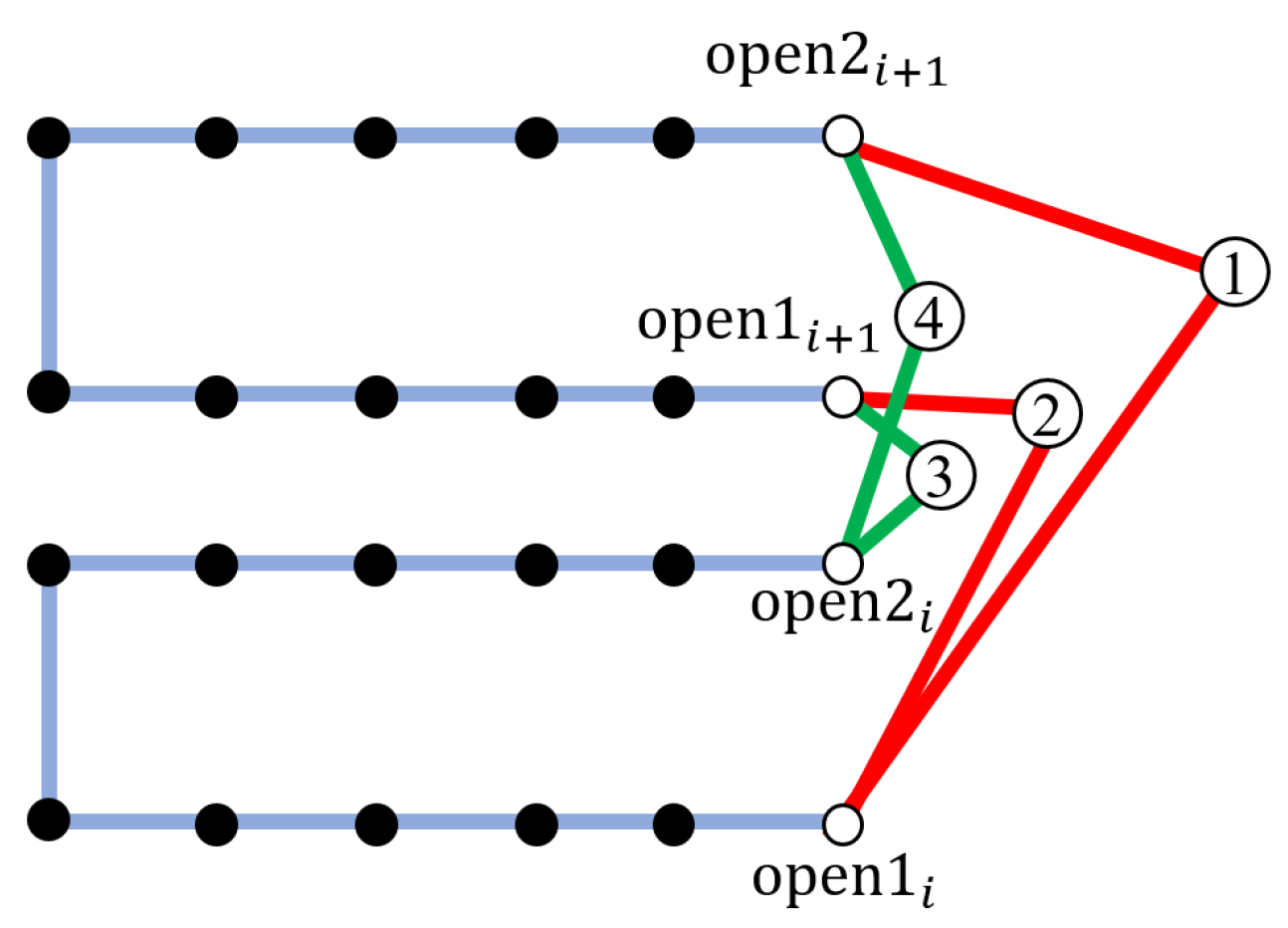
3.4. Inter-Layer Connection

Since the objective of the ADTSP is to minimize the inspection path length and the total turning angle, the inter-layer connections follow the same objective. However, the traversal direction significantly affects the total cost, particularly the turning angle cost. Therefore, the traversal direction is considered when estimating the total cost of different connection combinations. For the opening nodes at layer i, ${\mathrm{open}1}_i$ and ${\mathrm{open}2}_i$, and the opening nodes at layer $i+1$, ${\mathrm{open}1}_{i+1}$ and ${\mathrm{open}2}_{i+1}$, there are four possible connection combinations, as illustrated in Figure 3. The costs of all possible combinations are calculated, and the combination with the lowest cost is selected.

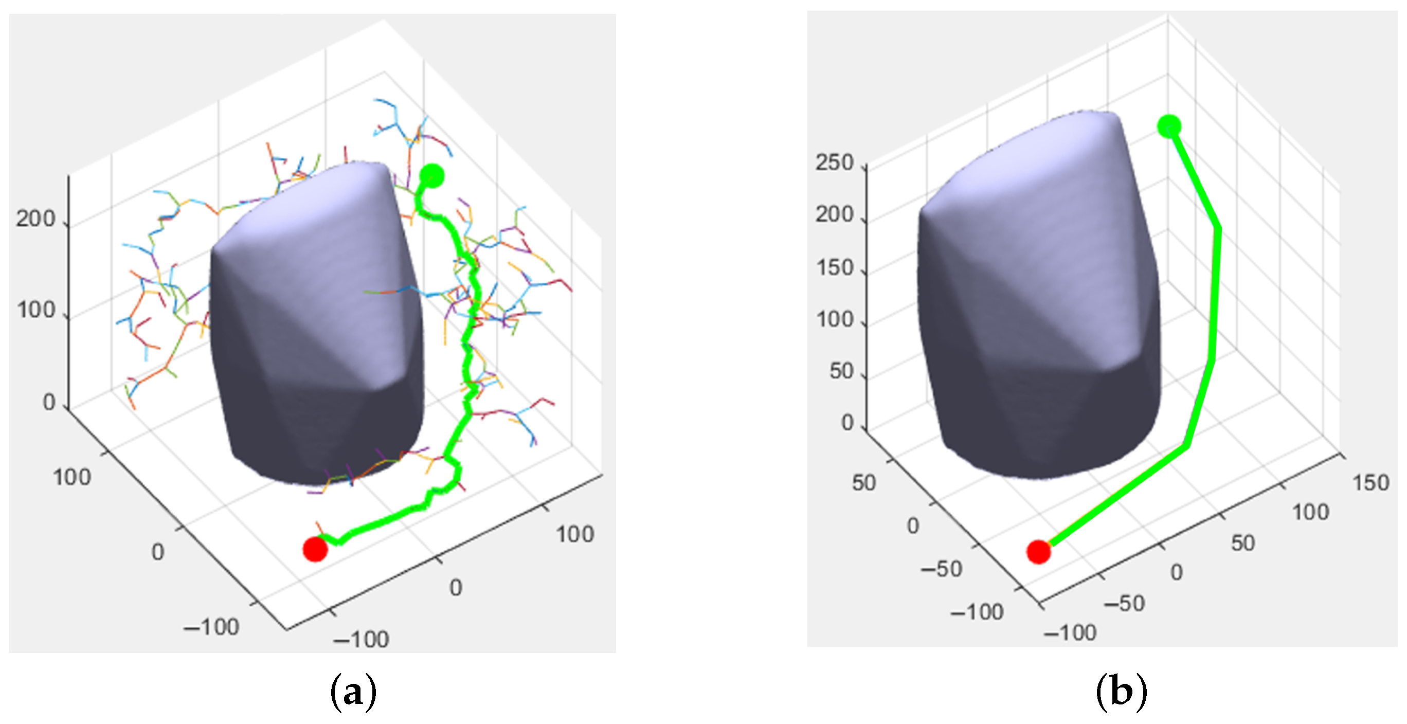
3.5. Collision Check

Since the ADTSP aims to find the optimal traversal sequence, possible collisions are not initially considered. Therefore, additional collision checks are required. With the ADTSP tours, collision checks are performed, and the collision paths are identified. In this paper, the Rapidly Exploring Random Tree (RRT) is selected as the local planner. However, the resulting path from the RRT may contain rapidly changing headings and redundant waypoints. Since the waypoints should be executable by the UAV directly, further processing is necessary.

A path simplification technique is employed to smooth the RRT path and remove any redundant waypoints. Algorithm 5 summarizes the smoothing algorithm. In the smoothing technique, the starting node is first selected. Collision checks are performed on all node pairs that include the starting node. The furthest collision-free node pair is selected, and the ending node of the pair is saved and designated as the current node. According to the triangle inequality, the sum of the distances of all intermediate paths will always be longer than the direct path connecting the two nodes. As a result, all intermediate nodes can be eliminated. Collision checks are then performed on the possible node pairs that include the current node. The iterations continue until the terminal node of the RRT path is reached. Using the simplification method, the number of waypoints in the RRT path can be significantly reduced while preserving the original traversal sequence computed by the ADTSP. Figure 4 illustrates the effect of the simplification process.

Algorithm 5 RRT Smoothening

Input: RRT Path $\mathit{Path}$ Output: Smoothened RRT Path ${\mathit{Path}}_{\mathit{s}}$ 1: $n_c\leftarrow Pat{h}_{start}$ 2: ${\mathit{Path}}_{\mathit{s}}\leftarrow$ Append $(Pat{h}_{start},{\mathit{Path}}_{\mathit{s}})$ 3: while true do 4:     for $i=n_c$ to $Pat{h}_{end}$ do 5:         if CollisionCheck($n_c,Pat{h}_i$) then 6:            $n_{next}\leftarrow Pat{h}_i$ 7:         end if 8:     end for 9:     ${\mathit{Path}}_{\mathit{s}}\leftarrow$ Append($n_{next},{\mathit{Path}}_{\mathit{s}}$) 10:    $n_c\leftarrow n_{next}$ 11:    if $n_{next}={\mathit{Path}}_{\mathit{end}}$ then 12:         break 13:    end if 14: end while 15: return ${\mathit{Path}}_{\mathit{s}}$

4. Simulation Results and Discussion

The performance of the proposed method is examined using various numerical simulations, starting with an analysis of the scalability of the proposed approach. Two infrastructures are used as inspection targets, each presenting different features that challenge the planning capabilities of the proposed algorithm: the Bank of China Tower in Hong Kong and Big Ben. The 3D models are in STL file format, and they are obtained through online library. To avoid excessive computation, the models are downscaled to reduce the number of surface patches while preserving the overall geometry. This is achieved using the isotropic explicit remeshing function of MeshLab [34]. To demonstrate the local scalability of the proposed method, both crack detection and photogrammetry are selected as inspection techniques, with detailed configurations summarized in

Table 2. Simulation configurations.

Inspection Method	Crack Detection	Photogrammetry
Max. Viewing Distance(m)	[10, 15]	[20, 25]
Field of View	${84}^{\circ }$	${84}^{\circ }$
Overlapping Rate, $\mu$	15	20
Viewing Angle, $\delta$	${60}^{\circ }$	${60}^{\circ }$
Coverage Requirement, $\epsilon$	1	3

. The simulations imitate the performance of the DJI Phantom 4 Pro V2, and the configurations of the onboard camera are obtained through calibration using a checkerboard. The simulation assumes that the inspection target is located in an open space, with no other structures present. Therefore, potential collisions with other structures are not considered. The mounted camera has three degrees of freedom: pitch, roll, and yaw. It should be noted that in practical applications, the camera’s degrees of freedom are limited, particularly the pitch, due to obstruction from the UAV’s body frame and blades. This issue can be mitigated by using a UAV equipped with a top-mounted camera, as demonstrated in [19]. The configurations of the GA used is summarized in

Table 3. Genetic Algorithm configurations.

Parameters	Value
Number of Generations, $N_G$	500
Population Size, $N_P$	300
Elitism Rate, $P_E$	0.05
Crossover Rate, $P_C$	0.7
Mutation Rate, $P_M$	0.3

. The simulation results are summarized in

Table 4. Simulation results.

	Number of Viewpoints		Traveling Distance (m)
Inspection Method	Model 1	Model 2	Model 1	Model 2
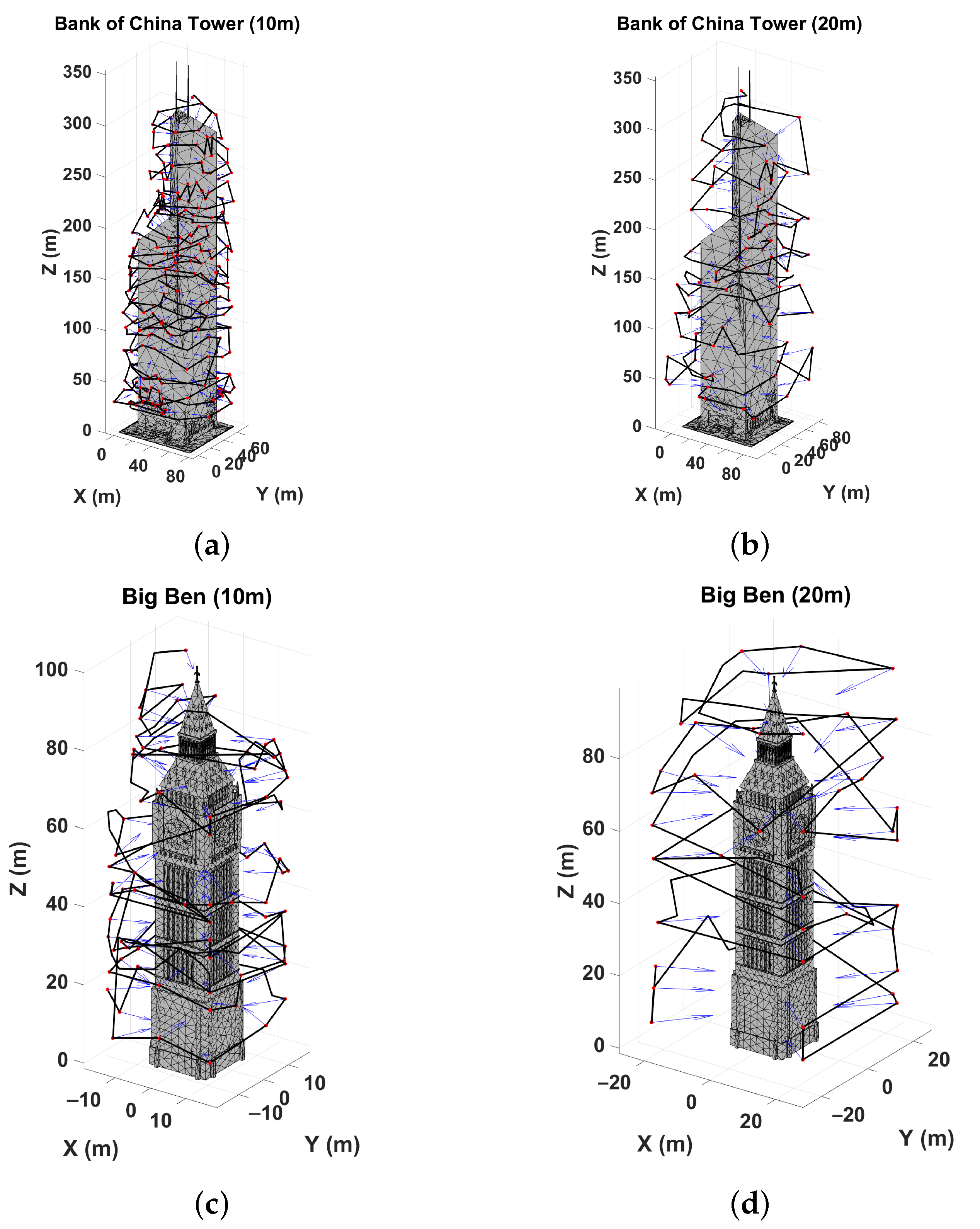
Crack Detection	290	87	5996	2202
Photogrammetry	87	47	3676	1768

and Figure 5.

The proposed method can generate a complete inspection for different models with different inspection methods while satisfying the corresponding coverage requirements. Model 1 contains large concave features that may challenge the view planning ability of the proposed method. While the uniformly generated revolving viewpoints may not be able to provide adequate coverage in those areas, the gap-filling viewpoints are able to compensate for the limitations of the revolving viewpoints by providing unique coverage at those areas. For Model 2, which contains more uniform surfaces, the revolving viewpoints provide the most coverage, and fewer gap-fill viewpoints are required, resulting in more uniformly distributed viewpoints. For the photogrammetry on both models, the revolving viewpoints provide adequate redundancy such that the overlapping requirements are met. Therefore, fewer gap-fill viewpoints are required. Different viewpoints contribute to the overall coverage of the different inspection methods. The simulation results again emphasize the importance of utilizing a mixed viewpoint generation technique to generate inspection paths that suit different inspection purposes. With the unified viewpoint generation method, the coverage requirements of different inspection methods can be met while maintaining information quality.

The proposed method can generate a comprehensive inspection for different models using various inspection methods while satisfying the corresponding coverage requirements. For Model 1, which features large concave areas that may challenge the view planning capabilities of the proposed method, the uniformly generated revolving viewpoints may not provide adequate coverage in those regions. However, the gap-filling viewpoints can compensate for the limitations of the revolving viewpoints by offering unique coverage in these areas. For Model 2, which has more uniform surfaces, the revolving viewpoints provide the most coverage, resulting in a reduced need for gap-fill viewpoints and a more uniformly distributed set of viewpoints. In terms of photogrammetry for both models, the revolving viewpoints offer sufficient redundancy to meet the overlapping requirements, thereby necessitating fewer gap-fill viewpoints.

Different viewpoints contribute significantly to the overall coverage of the various inspection methods. The simulation results further highlight the importance of employing a mixed viewpoint generation technique to create inspection paths tailored to different inspection purposes. With the unified viewpoint generation method, the coverage requirements of various inspection methods can be met while maintaining high information quality.

The effects of the ADTSP are then studied. The simulations were performed using the viewpoints generated for the photogrammetry of Big Ben. In the simulation, the performance of the ADTSP is compared to that of the ETSP. After dividing the viewpoints into different layers, the ADTSP and ETSP are solved. The minimum snap trajectory required to navigate through the inspection path is then estimated with a targeted velocity of $1{\mathrm{ms}}^{-1}$. The simulation results are summarized in

Table 5. Simulated results of the minimum snap trajectories. The bold value highlights the superior values.

	ML-ETSP	ML-ADTSP	% Change
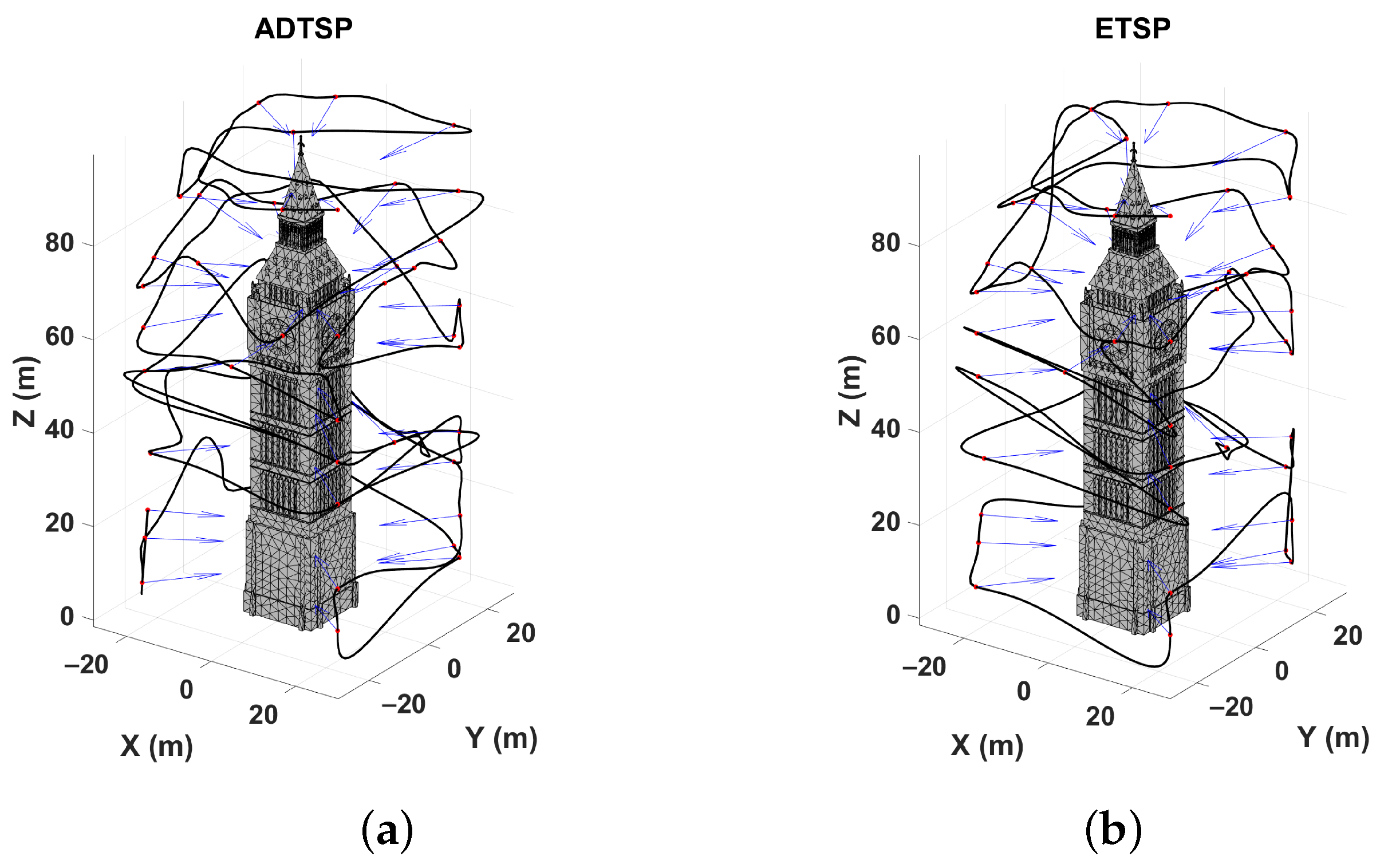
Mission Time (s)	1442	1768	$+22\%$
Mean Turning Angle (rad)	1.48	1.28	$-15\%$
Mean x-acceleration $\left({\mathrm{ms}}^{-2}\right)$	0.06	0.055	$-9\%$
Mean y-acceleration $\left({\mathrm{ms}}^{-2}\right)$	0.051	0.050	$-2\%$
Mean z-acceleration $\left({\mathrm{ms}}^{-2}\right)$	0.058	0.057	$-1.7\%$

and Figure 6 and Figure 7.

Since the objective of the ADTSP is to obtain a tour that minimizes both tour length and turning angle simultaneously, a tradeoff is observed. The resulting tour of the ADTSP shows an increased distance and mission time. However, with the increased tour length, the total turning angle is significantly reduced, with the ADTSP tour achieving a 15% reduction in turning angle. By minimizing the total turning angle, sharp turns are eliminated from the tour. Without sharp turns, the UAV can traverse through the viewpoints at a more consistent velocity, reducing the need for sudden acceleration and deceleration. The effect of the ADTSP can be observed in the mean accelerations of the simulated minimum snap trajectories. The ETSP exhibits higher mean accelerations across all three axes, while the ADTSP shows significant improvement. As noted earlier, acceleration induces energy consumption spikes that increase overall energy usage. Therefore, the ADTSP can lower overall energy consumption by reducing mean acceleration. A study of the overall acceleration indicates that the estimated acceleration of the ADTSP is smoother than that of the ETSP. With more consistent acceleration, the UAV can navigate through the viewpoints more comfortably, thereby reducing traversal difficulty.

More significant improvements are observed in areas with a high viewpoint density. In these locations, the ETSP tends to connect nearby nodes, often ignoring the turning angle of such connections. Consequently, the ETSP connections may contain sharp turns, increasing both traversal difficulty and energy consumption. While dense viewpoint distributions are inevitable, particularly in close-up inspections like crack detection, the ADTSP is essential for enhancing traversal smoothness. During this simulation, a relatively low traversal speed was selected, and significant improvements were noted (see Table 5). In scenarios where the UAV is required to travel at higher speeds, the impact of sharp turns would be even more pronounced, further highlighting the importance of the ADTSP. Additionally, the traversal order remains consistent in the low-level planning process. The simulation results demonstrate that to generate a more energy-efficient and less kinodynamically challenging path, fundamental dynamic constraints such as turning angle or altitude change should be incorporated during the preliminary planning phase.

5. Conclusions

This work addresses the path planning problem for complete structure inspection, emphasizing the scalability of viewpoint generation. A novel mixed-viewpoint generation method is proposed. Two practical application challenges are considered: coverage requirements and information quality. With unified viewpoint generation, the generated viewpoints can provide quality information for various inspection methods, such as crack detection and photogrammetry, which operate at different viewing distances. A novel ML-ADTSP is then introduced. The optimal viewpoint set obtained from the SCP is divided into different layers, limiting altitude changes along the inspection path. The ADTSP is solved locally within each layer, and the optimization function aims to minimize both the total tour length and turning angle simultaneously. By solving the ADTSP, the average acceleration of the inspection path is significantly reduced, which in turn decreases overall energy consumption and navigation difficulty. The importance of incorporating fundamental dynamic constraints during preliminary planning is highlighted by the simulation results. As for future work, the proposed system can be further enhanced by the following:

1.

Accurate viewpoint generation, which seeks to reduce overall computation time while maintaining scalability.

2.

Multi-agent inspection systems, aimed at reducing overall mission time and further improving information gain.

References

- Scott, W.R. Model-based view planning. Mach. Vis. Appl. 2009, 20, 47–69. [Google Scholar] [CrossRef]
- Alexis, K.; Papachristos, C.; Siegwart, R.; Tzes, A. Uniform coverage structural inspection path–planning for micro aerial vehicles. In Proceedings of the 2015 IEEE International Symposium on Intelligent Control (ISIC), Sydney, NSW, Australia, 21–23 September 2015; pp. 59–64. [Google Scholar] [CrossRef]
- Englot, B.; Hover, F.S. Sampling-based sweep planning to exploit local planarity in the inspection of complex 3D structures. In Proceedings of the 2012 IEEE/RSJ International Conference on Intelligent Robots and Systems, Vilamoura-Algarve, Portugal, 7–12 October 2012; pp. 4456–4463. [Google Scholar] [CrossRef]
- Tarbox, G.; Gottschlich, S. Planning for Complete Sensor Coverage in Inspection. Comput. Vis. Image Underst. 1995, 61, 84–111. [Google Scholar] [CrossRef]
- Jing, W.; Polden, J.; Lin, W.; Shimada, K. Sampling-based view planning for 3D visual coverage task with Unmanned Aerial Vehicle. In Proceedings of the 2016 IEEE/RSJ International Conference on Intelligent Robots and Systems (IROS), Daejeon, Republic of Korea, 9–14 October 2016; 2016; pp. 1808–1815. [Google Scholar] [CrossRef]
- Papachristos, C.; Alexis, K.; Carrillo, L.R.G.; Tzes, A. Distributed infrastructure inspection path planning for aerial robotics subject to time constraints. In Proceedings of the 2016 International Conference on Unmanned Aircraft Systems (ICUAS), Arlington, VA, USA, 7–10 June 2016; pp. 406–412. [Google Scholar] [CrossRef]
- Biundini, I.Z.; Pinto, M.F.; Melo, A.G.; Marcato, A.L.M.; Honório, L.M.; Aguiar, M.J.R. A Framework for Coverage Path Planning Optimization Based on Point Cloud for Structural Inspection. Sensors 2021, 21, 570. [Google Scholar] [CrossRef] [PubMed]
- Gu, W.; Hu, D.; Cheng, L.; Cao, Y.; Rizzo, A.; Valavanis, K.P. Autonomous Wind Turbine Inspection using a Quadrotor. In Proceedings of the 2020 International Conference on Unmanned Aircraft Systems (ICUAS), Athens, Greece, 1–4 September 2020; pp. 709–715. [Google Scholar] [CrossRef]
- Mansouri, S.S.; Kanellakis, C.; Fresk, E.; Kominiak, D.; Nikolakopoulos, G. Cooperative coverage path planning for visual inspection. Control Eng. Pract. 2018, 74, 118–131. [Google Scholar] [CrossRef]
- Almadhoun, R.; Taha, T.; Seneviratne, L.; Dias, J.; Cai, G. GPU accelerated coverage path planning optimized for accuracy in robotic inspection applications. In Proceedings of the 2016 IEEE 59th International Midwest Symposium on Circuits and Systems (MWSCAS), Abu Dhabi, United Arab Emirates, 16–19 October 2016; pp. 1–4. [Google Scholar] [CrossRef]
- Song, S.; Jo, S. Online inspection path planning for autonomous 3D modeling using a micro-aerial vehicle. In Proceedings of the 2017 IEEE International Conference on Robotics and Automation (ICRA), Singapore, 29 May–3 June 2017; pp. 6217–6224. [Google Scholar] [CrossRef]
- Cheng, P.; Keller, J.; Kumar, V. Time-optimal UAV trajectory planning for 3D urban structure coverage. In Proceedings of the 2008 IEEE/RSJ International Conference on Intelligent Robots and Systems, Nice, France, 22–26 September 2008; pp. 2750–2757. [Google Scholar] [CrossRef]
- Almadhoun, R.; Taha, T.; Dias, J.; Seneviratne, L.; Zweiri, Y. Coverage Path Planning for Complex Structures Inspection Using Unmanned Aerial Vehicle (UAV). In Intelligent Robotics and Applications; Springer: Cham, Switzerland, 2019; pp. 243–266. [Google Scholar] [CrossRef]
- Jing, W.; Deng, D.; Xiao, Z.; Liu, Y.; Shimada, K. Coverage Path Planning using Path Primitive Sampling and Primitive Coverage Graph for Visual Inspection. In Proceedings of the 2019 IEEE/RSJ International Conference on Intelligent Robots and Systems (IROS), Macau, China, 3–8 November 2019; pp. 1472–1479. [Google Scholar] [CrossRef]
- Jung, S.; Song, S.; Youn, P.; Myung, H. Multi-Layer Coverage Path Planner for Autonomous Structural Inspection of High-Rise Structures. In Proceedings of the 2018 IEEE/RSJ International Conference on Intelligent Robots and Systems (IROS), Madrid, Spain, 1–5 October 2018; pp. 1–9. [Google Scholar] [CrossRef]
- Jing, W.; Deng, D.; Wu, Y.; Shimada, K. Multi-UAV Coverage Path Planning for the Inspection of Large and Complex Structures. In Proceedings of the 2020 IEEE/RSJ International Conference on Intelligent Robots and Systems (IROS), Las Vegas, NV, USA, 24 October 2020–24 January 2021; pp. 1480–1486. [Google Scholar] [CrossRef]
- Freimuth, H.; König, M. Planning and executing construction inspections with unmanned aerial vehicles. Autom. Constr. 2018, 96, 540–553. [Google Scholar] [CrossRef]
- Jing, W.; Polden, J.; Tao, P.Y.; Lin, W.; Shimada, K. View planning for 3D shape reconstruction of buildings with unmanned aerial vehicles. In Proceedings of the 2016 14th International Conference on Control, Automation, Robotics and Vision (ICARCV), Phuket, Thailand, 13–15 November 2016; pp. 1–6. [Google Scholar] [CrossRef]
- Almadhoun, R.; Taha, T.; Gan, D.; Dias, J.; Zweiri, Y.; Seneviratne, L. Coverage Path Planning with Adaptive Viewpoint Sampling to Construct 3D Models of Complex Structures for the Purpose of Inspection. In Proceedings of the 2018 IEEE/RSJ International Conference on Intelligent Robots and Systems (IROS), Madrid, Spain, 1–5 October 2018; pp. 7047–7054. [Google Scholar] [CrossRef]
- Bircher, A.; Alexis, K.; Burri, M.; Oettershagen, P.; Omari, S.; Mantel, T.; Siegwart, R. Structural inspection path planning via iterative viewpoint resampling with application to aerial robotics. In Proceedings of the 2015 IEEE International Conference on Robotics and Automation (ICRA), Seattle, WA, USA, 26–30 May 2015; pp. 6423–6430. [Google Scholar] [CrossRef]
- Liu, X.; Yi, W.; Chen, P.; Tan, Y. Flight path planning of UAV-driven refinement inspection for construction sites based on 3D reconstruction. Autom. Constr. 2025, 177, 106360. [Google Scholar] [CrossRef]
- Zhang, J.; Zhu, X.; Li, J. Intelligent Path Planning with an Improved Sparrow Search Algorithm for Workshop UAV Inspection. Sensors 2024, 24. [Google Scholar] [CrossRef] [PubMed]
- Xu, W.; Cui, C.; Ji, Y.; Li, X.; Li, S. A UAV path planning algorithm for bridge construction safety inspection in complex terrain. Sci. Rep. 2025, 15, 13564. [Google Scholar] [CrossRef] [PubMed]
- Song, S.; Jo, S. Surface-Based Exploration for Autonomous 3D Modeling. In Proceedings of the 2018 IEEE International Conference on Robotics and Automation (ICRA), Brisbane, QLD, Australia, 21–25 May 2018; pp. 4319–4326. [Google Scholar] [CrossRef]
- Palazzolo, E.; Stachniss, C. Effective Exploration for MAVs Based on the Expected Information Gain. Drones 2018, 2, 9. [Google Scholar] [CrossRef]
- Rakha, T.; Gorodetsky, A. Review of Unmanned Aerial System (UAS) applications in the built environment: Towards automated building inspection procedures using drones. Autom. Constr. 2018, 93, 252–264. [Google Scholar] [CrossRef]
- Ellenberg, A.; Kontsos, A.; Bartoli, I.; Pradhan, A. Masonry Crack Detection Application of an Unmanned Aerial Vehicle. In Proceedings of the 2014 International Conference on Computing in Civil and Building Engineering, Orlando, FL, USA, 23–25 June 2014; Volume 93, pp. 1788–1795. [Google Scholar] [CrossRef]
- Yu, H.; Yang, W.; Zhang, H.; He, W. A UAV-based crack inspection system for concrete bridge monitoring. In Proceedings of the 2017 IEEE International Geoscience and Remote Sensing Symposium (IGARSS), Fort Worth, TX, USA, 23–28 July 2017; pp. 3305–3308. [Google Scholar] [CrossRef]
- Maes, W.H.; Huete, A.R.; Steppe, K. Optimizing the Processing of UAV-Based Thermal Imagery. Remote Sens. 2017, 9, 476. [Google Scholar] [CrossRef]
- Lee, E.J.; Shin, S.Y.; Ko, B.C.; Chang, C. Early sinkhole detection using a drone-based thermal camera and image processing. Infrared Phys. Technol. 2016, 78, 223–232. [Google Scholar] [CrossRef]
- Zulgafli, M.N.; Tahar, K.N. Three dimensional curve hall reconstruction using semi-automatic UAV. ARPN J. Eng. Appl. Sci. 2017, 12, 3228–3232. [Google Scholar]
- Haala, N.; Cramer, M.; Weimer, F.; Trittler, M. Performance Test on Uav-Based Photogrammetric Data Collection. Int. Arch. Photogramm. Remote Sens. Spatial Inf. Sci. 2011, XXXVIII-1/C22, 7–12. [Google Scholar] [CrossRef]
- Tong, H.W.; Li, B.; Huang, H.; Wen, C. UAV Path Planning for Complete Structural Inspection using Mixed Viewpoint Generation. In Proceedings of the 2022 17th International Conference on Control, Automation, Robotics and Vision (ICARCV), Singapore, 11–13 December 2022; pp. 727–732. [Google Scholar] [CrossRef]
- Cignoni, P.; Callieri, M.; Corsini, M.; Dellepiane, M.; Ganovelli, F.; Ranzuglia, G. MeshLab: An Open-Source Mesh Processing Tool. In Eurographics Italian Chapter Conference; The Eurographics Association: Eindhoven, The Netherlands, 2008; Volume 29, pp. 129–136. [Google Scholar] [CrossRef]
- Hartley, R.; Zisserman, A. Multiple View Geometry in Computer Vision; Cambridge University Press: Cambridge, UK, 2003. [Google Scholar]
- Abeywickrama, H.V.; Jayawickrama, B.A.; He, Y.; Dutkiewicz, E. Comprehensive Energy Consumption Model for Unmanned Aerial Vehicles, Based on Empirical Studies of Battery Performance. IEEE Access 2018, 6, 58383–58394. [Google Scholar] [CrossRef]
- Abeywickrama, H.V.; Jayawickrama, B.A.; He, Y.; Dutkiewicz, E. Empirical Power Consumption Model for UAVs. In Proceedings of the 2018 IEEE 88th Vehicular Technology Conference (VTC-Fall), Chicago, IL, USA, 27–30 August 2018; pp. 1–5. [Google Scholar] [CrossRef]
- Alyassi, R.; Khonji, M.; Karapetyan, A.; Chau, S.C.K.; Elbassioni, K.; Tseng, C.M. Autonomous Recharging and Flight Mission Planning for Battery-Operated Autonomous Drones. IEEE Trans. Autom. Sci. Eng. 2022, 20, 1034–1046. [Google Scholar] [CrossRef]
- Fischer, A.; Fischer, F.; Jäger, G.; Keilwagen, J.; Molitor, P.; Grosse, I. Exact algorithms and heuristics for the Quadratic Traveling Salesman Problem with an application in bioinformatics. Discret. Appl. Math. 2014, 166, 97–114. [Google Scholar] [CrossRef]
- Holland, J.H. Adaptation in Natural and Artificial Systems: An Introductory Analysis with Applications to Biology, Control, and Artificial Intelligence; MIT Press: Cambridge, UK, 1992. [Google Scholar]
- Larrañaga, P.; Kuijpers, C.; Murga, R.; Inza, I.; Dizdarevic, S. Genetic Algorithms for the Travelling Salesman Problem: A Review of Representations and Operators. Artif. Intell. Rev. 1990, 13, 129–170. [Google Scholar] [CrossRef]
- Alok, A.; Don, C.; Sanjeev, K.; Rajeev, M.; Baruch, S. The Angular-Metric Traveling Salesman Problem. SIAM J. Comput. 2000, 29, 697–711. [Google Scholar] [CrossRef]