Integral Backstepping Sliding Mode Control for Unmanned Autonomous Helicopters Based on Neural Networks

Abstract

In this paper, we propose an adaptive control approach to deal with the problems of input saturation, external disturbances, and uncertainty in the unmanned autonomous helicopter system. The dynamics of the system take into account the presence of input saturation, uncertainty, and external disturbances. Auxiliary systems are built to handle the input saturation. The neural networks are applied to approximate the uncertain terms. The control scheme combining integral backstepping and sliding mode control is developed in position and attitude subsystems, respectively. In the closed-loop system, the boundedness of the signals is proved by means of the Lyapunov theory. The simulation demonstrates that the approach has good robustness and tracking performance.

1. Introduction

Unmanned autonomous helicopters (UAHs) have received increasing attention in recent years due to their high cost-performance ratio and important contributions to surveillance, search, remote sensing, geographic research, and various military and security applications. UAHs have rotorcraft structures, enabling them to take off and land vertically, hover in the air, fly at low altitudes, and more. Due to their portability and flexibility, the application and research of miniature UAHs have rapidly developed. According to the rotor type, UAHs can be divided into single rotors with tail rotor types, coaxial rotor types, tilting rotor types, multi-rotor types, and so on [1]. Among them, conventional single-rotor UAHs with tail rotors are the most widely equipped nowadays. Their structures are simple and easy to operate. The main rotor is used to provide lift and the tail rotor is used to balance the reverse torque generated by the high-speed rotation of the main rotor. In this paper, we focus on the conventional single-rotor UAH with the tail rotor. Medium UAHs refer to UAHs with takeoff weights of 500–1000 kg [2], which have more load and endurance, better wind resistance, and anti-disturbance, and can perform more tasks that small helicopters cannot accomplish. These advantages make medium UAHs have broader application prospects in various fields. As a typical nonlinear strongly coupled underactuated system, the UAH system inevitably suffers from various disturbances and uncertain factors in the flight environment, such as model parameter changes, gust disturbances, air circulation, etc. These adverse effects may cause flight performance degradation or even loss of the stability provided by the control system. All of these bring challenges to the design of high-quality UAH controllers. Therefore, it is of crucial theoretical and engineering practical significance to investigate the applications of advanced control methods to UAH flight control systems.

With the booming development of control theory, many theoretical approaches have been widely applied to UAH flight control. Among linear control methods, PID control has played an important role due to its simple design process and independence from an accurate mathematical model [3,4]. In addition, $H_{\infty }$ control [5], linear quadratic regulator (LQR) [6], $\mu$-synthesis control [7], and fuzzy control [8] have also been implemented in flight control. Unlike the linear controller, which only considers the system performance near the operating point, the control method based on a nonlinear dynamics model has become a research hotspot for flight control. In existing literature studies, most research studies and applications of nonlinear UAH controls concentrate on dynamic inversion [9,10], feedback linearization [11,12], the backstepping technique, sliding mode control, and so on.

As a classical recursive design method for nonlinear feedback systems, the backstepping technique benefits from its systematic design process and has been utilized in various control systems. The authors of reference [13] designed an adaptive backstepping method for the UAH system with parameter uncertainties to track the upper reference trajectory. In [14], the attitude and altitude tracking controls were studied for the UAH based on the backstepping method. Reference [15] took a class of UAHs modeled by the rotation matrix as the research object and designed an adaptive backstepping tracking controller. On the premise of accomplishing various practical aviation tasks, an adaptive backstepping-based controller was designed in [16] for UAH; it makes the system stable and ensures the tracking of the reference trajectory. The integral backstepping method is improved on the basis of the traditional backstepping method by adding the integral term of the tracking error, which can compensate for the steady-state error and ensure the high precision of control [17]. It combines integration and backstepping to make the system robustness stronger [18].

The sliding mode control (SMC), which is also known as the sliding mode variable structure control, has been successfuly applied in nonlinear underactuated systems because of its simplicity and insensitivity to parameter changes and disturbances [19,20,21,22,23,24]. Unfortunately, the SMC’s disadvantages include discontinuous control signals and chattering. Given the characteristics of the SMC and integral backstepping, the advantages of the two methods can be combined to modify the controller. In [25], a controller that combines integral backstepping and SMC was developed to solve the control problem of the wagon–pendulum system. The results show that the controller can suppress disturbances well. This control method was also proposed to figure out trajectory tracking control for a quadrotor in [26]. It has obvious advantages in robustness to uncertain disturbances and tracking accuracy. However, the application of this method to UAHs is still relatively rare. As universal function approximation tools, neural networks (NNs) are popular in dealing with the uncertainties of nonlinear systems. The control scheme that combines NNs with other conventional control approaches has rapidly developed in UAHs [27,28,29]. An adaptive observer based on NN and the extended Kalman filter was designed to detect faults in [30], while an active fault-tolerant control was proposed on this basis so that the helicopter could track the target trajectory uninterruptedly. In [31], a new multivariable finite-time disturbance observer combined with NNs was investigated to process the disturbance and uncertainty; it was applied to the tracking control of the unmanned helicopter formation. NN was introduced to deal with the uncertainty and input dead zone of the helicopter system in [32]. An adaptive safe tracking control was realized in [33] by combining NN and the disturbance observer.

In the UAH system, the control input saturation cannot be avoided due to the physical condition of the actuator [34]. Input saturation can affect the control performance and lead to unacceptable control errors in severe cases. From the perspective of system security, input saturation is a hot research topic, and there have been many research studies in recent years. In [35], an adaptive neural tracking controller for a near-space vehicle was designed based on the backstepping method to cope with the input nonlinearity. In [36], auxiliary systems were adopted to deal with actuator saturation and faults; the reliability and safety operations of UAH were improved. An adaptive method was used for helicopters in [37] to compensate for the saturation error and external perturbation. System uncertainty, external disturbances, and input saturation should be considered when designing a control system. Therefore, the control design of a medium UAH requires further research.

Inspired by the above discussion, this paper presents an adaptive control for the UAH with input saturation, external disturbances, and uncertainty. The developed integral backstepping control strategy combined with NN and SMC avoids the discontinuity of control signals and improves tracking accuracy. The layout of the remaining contents is arranged as follows. Section 2 illustrates the simple theoretical analysis of modeling and presents the problems and preliminaries. In Section 3, an adaptive controller is built to guarantee the expected control performance. Some simulation results of the proposed control scheme are given in Section 4. Section 5 presents a summary of the main content.

2. Problem Formulation

The helicopter model is the basis of flight control design and the premise of simulation verification. Based on the previous research results, a simplified nonlinear mathematical model of a six-degree-of-freedom medium UAH was established. Firstly, the UAH is regarded as a symmetric rigid body with constant mass. Secondly, two coordinates frequently used in the modeling process are defined, namely the body’s fixed frame and the inertial frame. The motion forms of the UAH are mainly divided into translation motion and rotation motion. We define $P_e={[x,y,z]}^{\mathrm{T}}$ as the positional vector in the inertial coordinate system and $V_e={[u,v,w]}^{\mathrm{T}}$ as the translational velocity vector. We define $\Lambda ={[\varphi ,\theta ,\psi ]}^{\mathrm{T}}$ as the angle vector in the body-fixed frame and $\Omega ={[p,q,r]}^{\mathrm{T}}$ as the angular rate vector.

Then, the Newton–Euler equation is used to describe the dynamics of the UAH, which can be represented as [1,38]

$$\begin{array}{ccc}{\dot{P}}_e\hfill & =\hfill & V_e\hfill \\ {\dot{V}}_e\hfill & =\hfill & G+m^{-1}{R}_b^e{F}_b\hfill \\ \dot{\Lambda }\hfill & =\hfill & H\Omega \hfill \\ \dot{\Omega }\hfill & =\hfill & -I_n^{-1}\Omega \times I_n\Omega +I_n^{-1}{\Xi }_b\hfill \end{array}$$

(1)

where the mass of UAH is denoted by m and $G={[0,0,g]}^{\mathrm{T}}$; g means the gravitational acceleration. $F_b={\left[0,0,-T_m\right]}^{\mathrm{T}}$ and ${\Xi }_b={\left[L,M,N\right]}^{\mathrm{T}}$, respectively, represent the resultant external force vector and moment vector of the UAH. The inertia matrix is defined as $I_n=\mathrm{diag}\left\{I_{xx},I_{yy},I_{zz}\right\}$. The matrix $R_b^e$ is expressed as [1,38]

$$R_b^e=\left[\begin{array}{ccc}{T}_c\theta T_c\psi & T_s\varphi T_s\theta T_c\psi -T_c\varphi T_s\psi & T_s\varphi T_s\psi +T_c\varphi T_s\theta T_c\psi \\ T_s\psi T_c\theta & T_s\varphi T_s\theta T_s\psi +T_c\varphi T_c\psi & -T_s\varphi T_c\psi +T_c\varphi T_s\theta T_s\psi \\ -T_s\theta & T_s\varphi T_c\theta & T_c\varphi T_c\theta \end{array}\right],$$

(2)

which is the direction cosine converted from the body fixed frame to the inertial frame. Moreover, H is the attitude kinematic matrix defined as [1,38]

$$H=\left[\begin{array}{ccc}1& T_s\varphi T_t\theta & T_c\varphi T_t\theta \\ 0& T_c\varphi & -T_s\varphi \\ 0& T_s\varphi /T_c\theta & T_c\varphi /T_c\theta \end{array}\right].$$

(3)

The symbols $T_c$, $T_s$, and $T_t$ are abbreviations for the trigonometric functions cos, sin and tan, respectively.

We define $u_c={[T_m,L,M,N]}^{\mathrm{T}}$. The saturation function of the control input is expressed as [34]

$$\mathrm{sat}(u_{ci})=\left\{\begin{array}{cc}\mathrm{sign}(u_{ci}){\overline{u}}_{ci},& \left|u_{ci}\right|>{\overline{u}}_{ci}\\ u_{ci},& \left|u_{ci}\right|\le {\overline{u}}_{ci}\end{array}\right.$$

(4)

where $i=1,2,3,4$, and ${\overline{u}}_{ci}>0$ is the upper bound of the control signal.

To improve the control performance and reliability of the UAH system, the existence of system uncertainty, external disturbance, and control input saturation should be taken into account during modeling. Let $F_{bs}={\left[0,0,-\mathrm{sat}(T_m)\right]}^{\mathrm{T}}$, ${\Xi }_{bs}={\left[\mathrm{sat}(L),\mathrm{sat}(M),\mathrm{sat}(N)\right]}^{\mathrm{T}}$. The dynamics of the velocity/angular rate can be redefined as

$$\begin{array}{ccc}\hfill {\dot{V}}_e& =& G+\Delta G+m^{-1}{R}_b^e{F}_{bs}+d_1\hfill \end{array}$$

(5)

$$\begin{array}{ccc}\hfill \dot{\Omega }& =& f(\Omega )+\Delta f+I_n^{-1}{\Xi }_{bs}+d_2\hfill \end{array}$$

(6)

where $f(\Omega )=-I_n^{-1}\Omega \times I_n\Omega$, $\Delta G$, and $\Delta f$ are the system uncertainties, while $d_1$ and $d_2$ are external force type disturbance and torque type disturbance acting on the UAH, respectively.

The objective of the paper was to develop an adaptive control scheme for UAHs that can ensure the tracking of desired signals and the boundedness of signals in the overall closed-loop system in the presence of input saturation, uncertainty and external disturbances.

To facilitate the handling of the UAH system’s control problem, some relevant assumptions and lemmas need to be briefly described.

Assumption A1 ([14]). 

The pitch angle θ and roll angle ϕ are always kept within a reasonable range that satisfies the inequality constraints: $\left|\varphi \right|<\frac{\pi }{2}$ and $\left|\theta \right|<\frac{\pi }{2}$.

Assumption A2 ([39]). 

The external disturbances of the UAH $d_i(i=1,2)$ are bounded, i.e., $\parallel d_i\parallel \le \overline{d_i}$ with $\overline{d_i}>0$.

Assumption A3 ([40]). 

Both the desired trajectory $y_d$ and its derivatives ${\dot{y}}_d,{\ddot{y}}_d$ are all bounded. That is to say, there is a positive unknown constant $o_d$ satisfying $E_d:=\{(y_d,{\dot{y}}_d,{\ddot{y}}_d):{∥y_d∥}^2+{∥{\dot{y}}_d∥}^2+{∥{\ddot{y}}_d∥}^2\le o_d\}$, where $E_d$ is a compact set.

Assumption A4 ([34]). 

The difference between the desired input and the actual input caused by input saturation is bounded. In other words, $\Delta u_{ci}(i=1,2,3,4)$ satisfies the condition $∥\Delta u_{ci}∥\le {\sigma }_i$, where $\Delta u_{ci}$ is the difference expressed as $\Delta u_{ci}=\mathrm{sat}(u_{ci})-u_{ci}$ and ${\sigma }_i$ is an unknown positive constant.

Lemma 1 ([41]). 

For the studied UAH system, there exists $c_0>0$, $\kappa >0$, and a positive definite Lyapunov function $V(x)$ that satisfies a few conditions: (1) the initial value is bounded; (2) ${\gamma }_1(\parallel x\parallel )\le V(x)\le {\gamma }_2(\parallel x\parallel )$, where ${\gamma }_1,{\gamma }_2:R^n\to R$ are class K functions; (3) $\dot{V}(x)\le -\kappa V(x)+c_0$. Consequently, the solution $x(t)$ is uniformly bounded.

Lemma 2 ([42]). 

The radial basis function NN (RBFNN) is a popular feedforward NN, and its strong nonlinear mapping ability makes it widely utilized in various uncertain nonlinear systems. RBFNN can be frequently employed to estimate a continuous function $\lambda (Z):R^q\to R$; its expression is as follows:

$$\lambda (Z)={\widehat{\Theta }}^{\mathrm{T}}\Pi (Z)+\zeta$$

(7)

where Z means the input vector, ζ is the approximation error and satisfies the conditions $\left|\zeta \right|\le \overline{\zeta }$, and $\overline{\zeta }>0$ is an unknown constant. $\widehat{\Theta }$ means the weight vector, and $\Pi (Z)$ is the basis function (generally picked as the Gaussian function).

Obviously, the function $\lambda (Z)$ on the compact set ${\Omega }_Z$ can be approximated by RBFNN with any precision as

$$\lambda (Z)={\Theta }^{\ast \mathrm{T}}\Pi (Z)+{\zeta }^{\ast }$$

(8)

where ${\zeta }^{\ast }$ represents the minimum approximation error. ${\Theta }^{\ast }$ is the optimal weight value expressed as

$${\Theta }^{\ast }=arg\underset{\widehat{\Theta }\in R^p}{min}\left[\underset{Z\in {\Omega }_Z}{sup}\left|\widehat{\lambda }(Z|\widehat{\Theta })-\lambda (Z)\right|\right]$$

(9)

Remark 1. 

When the UAH is hovering or flying horizontally at a low speed, the flapping angle of the main rotor is small. The lift of the main rotor is regarded as the primary control unit for the position loop, while torque (in the three directions of the body coordinate system) is used for attitude control. During actual flight, operators primarily balance forces and torques on the UAH by controlling two collective pitch inputs generated by the tail rotor and main rotor, as well as longitudinal and transverse periodic pitch inputs produced by the main rotor, to maintain stable flight.

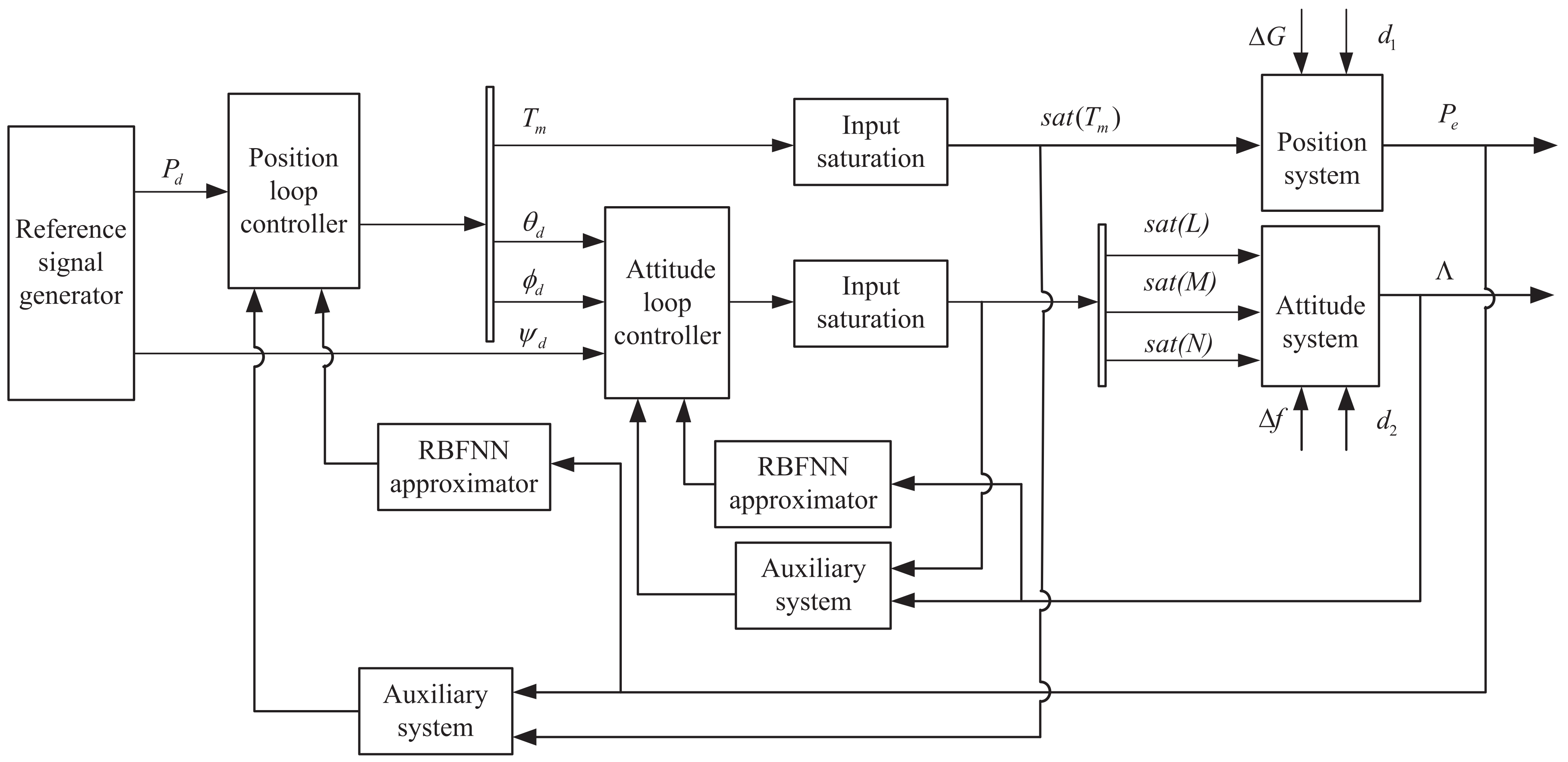
3. Controller Design of the UAH with Input Saturation, Disturbances and Uncertainty

In this section, an adaptive control scheme for the UAH is proposed to track the target trajectory, which is based on integral backstepping and the SMC. Moreover, it can reduce the impact of input saturation, disturbances and uncertainty on the system performance. The control of the position loop and attitude loop are considered separately. The control design flow is given in Figure 1.

3.1. Positional Subsystem Controller

Firstly, the control scheme for the position loop is given. The detailed design steps are as follows.

An auxiliary system is built to handle the input saturation as follows [35]:

$$\left\{\begin{array}{c}{\dot{\xi }}_1=-{\kappa }_1{\xi }_1+{\xi }_2\hfill \\ {\dot{\xi }}_2=-{\kappa }_2{\xi }_2-{\xi }_1+m^{-1}{R}_b^e\Delta u_1\hfill \end{array}\right.$$

(10)

where $\Delta u_1=F_{bs}-F_b$, ${\xi }_1$ and ${\xi }_2$ are state variables of the auxiliary system, ${\kappa }_1$ and ${\kappa }_2$ are diagonal and positive definite matrices.

In combination with the designed auxiliary system, we define the positional tracking error as

$$e_1=P_e-P_d-{\xi }_1+K_1\int (P_e-P_d-{\xi }_1)dt$$

(11)

where $P_d$ is the desired position, and $K_1\in R^{3\times 3}$ is an integral coefficient diagonal matrix that is positive definite.

The Lyapunov function is selected as:

$$V_1=\frac{1}{2}{e}_1^{\mathrm{T}}{e}_1$$

(12)

We define the velocity error as

$$e_2=V_e-{\alpha }_1-{\xi }_2$$

(13)

where ${\alpha }_1$ is the virtual control law to be designed.

Invoking (13) and taking the time derivative of $V_1$, we have

$$\begin{array}{ccc}\hfill {\dot{V}}_1& =& e_1^{\mathrm{T}}{\dot{e}}_1\hfill \\ & =& e_1^{\mathrm{T}}(V_e-{\dot{P}}_d-{\dot{\xi }}_1+K_1\left(P_e-P_d-{\xi }_1\right))\hfill \\ & =& e_1^{\mathrm{T}}(e_2+{\alpha }_1+{\xi }_2-{\dot{P}}_d-{\dot{\xi }}_1+K_1\left(P_e-P_d-{\xi }_1\right))\hfill \\ & =& e_1^{\mathrm{T}}(e_2+{\alpha }_1-{\dot{P}}_d+{\kappa }_1{\xi }_1+K_1(P_e-P_d-{\xi }_1))\hfill \end{array}$$

(14)

Then, we propose the virtual control input as

$${\alpha }_1={\dot{P}}_d-A_1{e}_1-{\kappa }_1{\xi }_1-K_1\left(P_e-P_d-{\xi }_1\right)$$

(15)

where $A_1=A_1^{\mathrm{T}}\in R^{3\times 3}$ is a positive definite matrix.

Thus, we substitute (15) into (14) to obtain

$${\dot{V}}_1=-e_1^{\mathrm{T}}{A}_1{e}_1+e_1^{\mathrm{T}}{e}_2$$

(16)

From (5), we know that the position subsystem is uncertain. To solve the difficulty, a RBFNN is applied to estimate the unknown uncertainty $\Delta G$ with the precision of minimum approximation error ${\zeta }_1$, which is written as [42]

$$\Delta G={\Theta }_1^{\ast \mathrm{T}}\Pi (x_1)+{\zeta }_1$$

(17)

where $x_1={[P_e^{\mathrm{T}},V_e^{\mathrm{T}}]}^{\mathrm{T}}$, ${\zeta }_1$ satisfies $\parallel {\zeta }_1\parallel \le \overline{{\zeta }_1}$, $\overline{{\zeta }_1}>0$ is an unknown constant, and ${\Theta }_1^{\ast }$ denotes the optimal weight of RBFNN.

By substituting (17) into (5), we have

$${\dot{V}}_e=G+{\Theta }_1^{\ast \mathrm{T}}\Pi (x_1)+m^{-1}{R}_b^e{F}_{bs}+{\epsilon }_1$$

(18)

where ${\epsilon }_1={\zeta }_1+d_1$. Combining Assumption 2 with Lemma 2, we have $\parallel {\epsilon }_1\parallel \le {\delta }_1$, and a positive constant ${\delta }_1$ is the upper bound.

We consider the following sliding surface:

$$\begin{array}{ccc}\hfill s_1& =& e_2\hfill \\ & =& V_e-\left({\dot{P}}_d-A_1{e}_1-{\kappa }_1{\xi }_1-K_1\left(P_e-P_d-{\xi }_1\right)\right)-{\xi }_2\hfill \\ & =& {\dot{P}}_e-{\dot{P}}_d-{\dot{\xi }}_1+K_1\left(P_e-P_d-{\xi }_1\right)+A_1{e}_1\hfill \\ & =& {\dot{e}}_1+A_1{e}_1\hfill \end{array}$$

(19)

Invoking (10), (15) and (18), the time derivative of $s_1$ is

$$\begin{array}{ccc}\hfill {\dot{s}}_1& =& {\dot{V}}_e-{\dot{\alpha }}_1-{\dot{\xi }}_2\hfill \\ & =& G+{\Theta }_1^{\ast \mathrm{T}}\Pi (x_1)+m^{-1}{U}_1+{\epsilon }_1-{\dot{\alpha }}_1+{\kappa }_2{\xi }_2+{\xi }_1\hfill \end{array}$$

(20)

where $U_1=R_b^e{F}_b$.

The dynamic surface control technique is applied to overcome differential explosion and obtain the derivative of the virtual control input. Pass ${\alpha }_1$ through the first-order filter to obtain $a_1$ as follow [34]:

$$r_1{\dot{a}}_1+a_1={\alpha }_1,a_1(0)={\alpha }_1(0)$$

(21)

where $r_1$ is a time constant matrix that satisfies $r_1=diag\{r_{11},r_{12},r_{13}\}>0$.

Defining $e_{\alpha 1}=a_1-{\alpha }_1$, we have

$${\dot{e}}_{\alpha 1}={\dot{a}}_1-{\dot{\alpha }}_1=-r_1^{-1}{e}_{\alpha 1}+N_1({\dot{P}}_d,{\xi }_1,e_1)$$

(22)

where $N_1({\dot{P}}_d,{\xi }_1,e_1)=-(\partial {\alpha }_1/\partial P_d){\dot{P}}_d-(\partial {\alpha }_1/\partial {\xi }_1){\dot{\xi }}_1-(\partial {\alpha }_1/\partial e_1){\dot{e}}_1$ represents the sufficiently smooth function vector. According to assumption 3, $N_1\left(•\right)$ is bounded under the given initial condition, which is satisfied $∥N_1\left(•\right)∥\le {\overline{N}}_1,{\overline{N}}_1>0$ [43].

The candidate Lyapunov function is

$$V_2=\frac{1}{2}{e}_1^{\mathrm{T}}{e}_1+\frac{1}{2}{s}_1^{\mathrm{T}}{s}_1+\frac{1}{2}tr({\tilde{\Theta }}_1^{\mathrm{T}}{\Gamma }_1^{-1}{\tilde{\Theta }}_1)+\frac{1}{2}\sum _{i=1}^2{\xi }_i^{\mathrm{T}}{\xi }_i+\frac{1}{2}{e}_{\alpha }^{\mathrm{T}}{e}_{\alpha }$$

(23)

where ${\tilde{\Theta }}_1={\widehat{\Theta }}_1-{\Theta }_1^{\ast }$, ${\Gamma }_1>0$ is a diagonal matrix to be computed.

Its time derivative is

$$\begin{array}{ccc}\hfill {\dot{V}}_2& =& e_1^{\mathrm{T}}{\dot{e}}_1+s_1^{\mathrm{T}}{\dot{s}}_1+tr({\tilde{\Theta }}_1^{\mathrm{T}}{\Gamma }_1^{-1}{\dot{\tilde{\Theta }}}_1)+{\xi }_1^{\mathrm{T}}{\dot{\xi }}_1+{\xi }_2^{\mathrm{T}}{\dot{\xi }}_2+e_{\alpha }^{\mathrm{T}}{\dot{e}}_{\alpha }\hfill \\ & =& e_1^{\mathrm{T}}\left(-A_1{e}_1+s_1\right)+s_1^{\mathrm{T}}({\dot{V}}_e-{\dot{\alpha }}_1-{\dot{\xi }}_2)+tr({\tilde{\Theta }}_1^{\mathrm{T}}{\Gamma }_1^{-1}{\dot{\widehat{\Theta }}}_1)+{\xi }_1^{\mathrm{T}}{\dot{\xi }}_1+{\xi }_2^{\mathrm{T}}{\dot{\xi }}_2+e_{\alpha 1}^{\mathrm{T}}{\dot{e}}_{\alpha 1}\hfill \\ & =& e_1^{\mathrm{T}}\left(-A_1{e}_1+s_1\right)+s_1^{\mathrm{T}}(G+{\Theta }_1^{\ast \mathrm{T}}\Pi (x_1)+m^{-1}{U}_1+{\epsilon }_1-{\dot{\alpha }}_1+{\kappa }_2{\xi }_2+{\xi }_1)\hfill \\ & & +tr({\tilde{\Theta }}_1^{\mathrm{T}}{\Gamma }_1^{-1}{\dot{\widehat{\Theta }}}_1)-{\xi }_1^{\mathrm{T}}{\kappa }_1{\xi }_1-{\xi }_2^{\mathrm{T}}{\kappa }_2{\xi }_2+{\xi }_2^{\mathrm{T}}(m^{-1}{R}_b^e\Delta u_1)+e_{\alpha }^{\mathrm{T}}{\dot{e}}_{\alpha }\hfill \end{array}$$

(24)

The control input of the position subsystem is

$$U_1=m(-G-e_1+{\dot{a}}_1-{\kappa }_2{\xi }_2-{\xi }_1-{\eta }_1\mathrm{Sign}(s_1)-T_1{s}_1-{\widehat{\Theta }}_1^{\mathrm{T}}\Pi (x_1))$$

(25)

where $T_1>0$ is a designed diagonal matrix, and ${\eta }_1$ is a parameter satisfying ${\eta }_1-∥{\epsilon }_1∥\ge 0$. $\mathrm{Sign}(s_1)={[\mathrm{sign}(s_{11}),\mathrm{sign}(s_{12}),\mathrm{sign}(s_{13})]}^{\mathrm{T}}$, and the definition of the sign function is

$$\mathrm{sign}(\upsilon )=\left\{\begin{array}{c}\begin{array}{cc}1,& \upsilon >0\end{array}\hfill \\ \begin{array}{cc}0,& \upsilon =0\end{array}\hfill \\ \begin{array}{cc}-1,& \upsilon <0\end{array}\hfill \end{array}\right.$$

(26)

Remark 2. 

Due to the discontinuous switching on the sliding mode surface, high frequency chattering exists in the SMC. To smooth the control signal, in (25), the hyperbolic tangent function can be selected to replace the sign function, which is defined as

$$tanh(\upsilon )=\frac{-e^{-\upsilon }+e^{\upsilon }}{e^{-\upsilon }+e^{\upsilon }}$$

(27)

Thus, to avoid chattering, the control low is rewritten as

$$U_1=m(-G-e_1+{\dot{a}}_1-{\kappa }_2{\xi }_2-{\xi }_1-{\eta }_1\mathrm{Tanh}(s_1)-T_1{s}_1-{\widehat{\Theta }}_1^{\mathrm{T}}\Pi (x_1))$$

(28)

where $\mathrm{Tanh}(s_1)={[\tanh (s_{11}),\tanh (s_{12}),\tanh (s_{13})]}^{\mathrm{T}}$.

The adaptive update law for ${\dot{\widehat{\Theta }}}_1$ is designed as

$${\dot{\widehat{\Theta }}}_1={\Gamma }_1(\Pi (x_1)s_1^{\mathrm{T}}-{\tau }_1{\widehat{\Theta }}_1)$$

(29)

where ${\tau }_1>0$ is a design parameter.

We substitute (10), (28), and (29) into (24) to obtain

$$\begin{array}{ccc}\hfill {\dot{V}}_2& =& -e_1^{\mathrm{T}}{A}_1{e}_1+s_1^{\mathrm{T}}{\epsilon }_1+s_1{\dot{e}}_{\alpha 1}-s_1^{\mathrm{T}}{\eta }_1\mathrm{Tanh}\left(s_1\right)-s_1^{\mathrm{T}}{T}_1{s}_1-{\tau }_{1}tr({\tilde{\Theta }}_1^{\mathrm{T}}{\widehat{\Theta }}_1)-{\xi }_1^{\mathrm{T}}{\kappa }_1{\xi }_1\hfill \\ & & -{\xi }_2^{\mathrm{T}}{\kappa }_2{\xi }_2+{\xi }_2^{\mathrm{T}}(m^{-1}{R}_b^e\Delta u_1)+e_{\alpha 1}^{\mathrm{T}}{\dot{e}}_{\alpha 1}\hfill \end{array}$$

(30)

We define $\beta =\mathrm{Sign}(s_1)-\mathrm{Tanh}(s_1)$. Then, we obtain

$$\begin{array}{ccc}\hfill {\dot{V}}_2& =& -e_1^{\mathrm{T}}{A}_1{e}_1+s_1^{\mathrm{T}}{\epsilon }_1+s_1{\dot{e}}_{\alpha 1}-s_1^{\mathrm{T}}{\eta }_1(\mathrm{Sign}(s_1)-\beta )-s_1^{\mathrm{T}}{T}_1{s}_1-{\tau }_{1}tr({\tilde{\Theta }}_1^{\mathrm{T}}{\widehat{\Theta }}_1)-{\xi }_1^{\mathrm{T}}{\kappa }_1{\xi }_1\hfill \\ & & -{\xi }_2^{\mathrm{T}}{\kappa }_2{\xi }_2+{\xi }_2^{\mathrm{T}}(m^{-1}{R}_b^e\Delta u_1)+e_{\alpha 1}^{\mathrm{T}}{\dot{e}}_{\alpha 1}\hfill \\ & \le & -e_1^{\mathrm{T}}{A}_1{e}_1+s_1{\dot{e}}_{\alpha 1}+s_1^{\mathrm{T}}{\eta }_1\beta -s_1^{\mathrm{T}}{T}_1{s}_1-{\tau }_{1}tr({\tilde{\Theta }}_1^{\mathrm{T}}{\widehat{\Theta }}_1)-{\xi }_1^{\mathrm{T}}{\kappa }_1{\xi }_1-{\xi }_2^{\mathrm{T}}{\kappa }_2{\xi }_2\hfill \\ & & +{\xi }_2^{\mathrm{T}}(m^{-1}{R}_b^e\Delta u_1)+e_{\alpha 1}^{\mathrm{T}}{\dot{e}}_{\alpha 1}\hfill \end{array}$$

(31)

Consider the following inequalities

$$\begin{array}{ccc}\hfill -{\tau }_{1}tr({\tilde{\Theta }}_1^{\mathrm{T}}{\widehat{\Theta }}_1)& \le & -\frac{1}{2}{\tau }_1\parallel {\tilde{\Theta }}_1{\parallel }^2+\frac{1}{2}{\tau }_1\parallel {\Theta }_1^{\ast }{\parallel }^2\hfill \\ \hfill s_1^{\mathrm{T}}{\eta }_1\beta & \le & {\eta }_1\rho ∥s_1∥\le \frac{b}{2}{\eta }_1^2{\rho }^2{s}_1^{\mathrm{T}}{s}_1+\frac{1}{2b}\hfill \\ \hfill {\xi }_2^{\mathrm{T}}(m^{-1}{R}_b^e\Delta u_1)& \le & \frac{1}{2o_1}{\mathrm{B}}_1^2+\frac{o_1}{2}{\xi }_2^{\mathrm{T}}{\xi }_2\hfill \\ \hfill s_1{\dot{e}}_{\alpha 1}& \le & s_1^{\mathrm{T}}(\frac{1}{2}{∥r_1^{-1}∥}^2+\frac{1}{2})s_1+\frac{1}{2}{e}_{\alpha 1}^{\mathrm{T}}{e}_{\alpha 1}+\frac{1}{2}{\overline{N}}_1^2\hfill \end{array}$$

(32)

where $∥\beta ∥=∥\mathrm{Sign}(s_1)-\mathrm{Tanh}(s_1)∥\le \rho ,0\le \rho \le 2\sqrt{3}$, $∥m^{-1}{R}_b^e\Delta u_1∥\le {\mathrm{B}}_1$, b and $o_1$ are positive constants.

Substituting (32) into (31), we have

$$\begin{array}{ccc}\hfill {\dot{V}}_2& \le & -e_1^{\mathrm{T}}{A}_1{e}_1-s_1^{\mathrm{T}}(T_1-(\frac{b}{2}{\eta }_1^2{\rho }^2+\frac{1}{2}{∥r_1^{-1}∥}^2+\frac{1}{2})I)s_1-\frac{{\tau }_1}{2}{∥{\tilde{\Theta }}_1∥}^2\hfill \\ & & -{\xi }_1^{\mathrm{T}}{\kappa }_1{\xi }_1-{\xi }_2^{\mathrm{T}}({\kappa }_2-\frac{o_1}{2}I)\xi -e_{\alpha 1}^{\mathrm{T}}(r_1^{-1}-I)e_{\alpha 1}\hfill \\ & & +\frac{{\tau }_1}{2}{∥{\Theta }_1^{\ast }∥}^2+\frac{1}{2b}+\frac{1}{2o_1}{\mathrm{B}}_1^2+{\overline{N}}_1^2\hfill \end{array}$$

(33)

3.2. Attitude Subsystem Controller

The UAH is a typical underactuated system that has four inputs but six outputs. For the attitude subsystem and position subsystem, coupling exists between the two. So the yaw angle ${\psi }_d$ is given as a predetermined value, and the remaining two attitude angles need to be solved by the following formula [44]

$$\left\{\begin{array}{c}{\varphi }_d=arctan\left(\frac{cos{\theta }_d(u_{x}sin{\psi }_d-u_{y}cos{\psi }_d)}{u_z}\right)\hfill \\ {\theta }_d=arctan\left(\frac{u_{x}cos{\psi }_d+u_{y}sin{\psi }_d}{u_z}\right)\hfill \end{array}\right.$$

(34)

where the control input $U_1$ is written as $U_1={[u_x,u_y,u_z]}^{\mathrm{T}}$.

Through the inverse solution of formula $U_1=R_b^e{F}_b$ and the controller (28), the main rotor lift can be described as

$$T_m=\frac{u_z}{cos{\varphi }_{d}cos{\theta }_d}$$

(35)

In this subsection, the control scheme of the attitude system is similar to the previous subsystem. The dynamic surface method is applied to process the desired signal.

We define the expected value ${\Lambda }_d={[{\varphi }_d,{\theta }_d,{\psi }_d]}^{\mathrm{T}}$. In order to avoid the variable unavailability and differential explosion caused by multiple derivatives, we adopt the dynamic surface technique to obtain its available derivative. We pass ${\Lambda }_d$ through the first-order filter to obtain ${\lambda }_d$ as follows [34]:

$$\gamma {\dot{\lambda }}_d+{\lambda }_d={\Lambda }_d,\lambda (0)={\Lambda }_d(0)$$

(36)

where $\gamma$ is the time constant matrix that satisfies $\gamma =\mathrm{diag}\{{\gamma }_1,{\gamma }_2,{\gamma }_3\}>0$.

Defining $e_f={\lambda }_d-{\Lambda }_d$, we have

$${\dot{e}}_f={\dot{\lambda }}_d-{\dot{\Lambda }}_d=-{\gamma }^{-1}{e}_f+M(a_1,e_1,s_1,{\xi }_1,{\xi }_2)$$

(37)

where $M(a_1,e_1,s_1,{\xi }_1,{\xi }_2)=-(\partial {\Lambda }_d/\partial a_1){\dot{a}}_1-(\partial {\Lambda }_d/\partial e_1){\dot{e}}_1-(\partial {\Lambda }_d/\partial s_1){\dot{s}}_1-(\partial {\Lambda }_d/\partial {\xi }_1){\dot{\xi }}_1-(\partial {\Lambda }_d/\partial {\xi }_2){\dot{\xi }}_2$ represents the sufficiently smooth function vector. According to Assumption 3, $M\left(•\right)$ is bounded under the given initial condition, which is satisfied $∥M\left(•\right)∥\le \overline{M},\overline{M}>0$ [43].

To handle the input saturation, another auxiliary system is constructed as follows [35]:

$$\left\{\begin{array}{c}{\dot{\xi }}_3=-{\kappa }_3{\xi }_3+H{\xi }_4\hfill \\ {\dot{\xi }}_4=-{\kappa }_4{\xi }_4-H^{\mathrm{T}}{\xi }_3+H{I}_n^{-1}\Delta \Xi \hfill \end{array}\right.$$

(38)

where $\Delta \Xi ={\Xi }_{bs}-{\Xi }_b$, ${\xi }_3$, and ${\xi }_4$ are internal states of the auxiliary system, and ${\kappa }_3$ and ${\kappa }_4$ are diagonal and positive-definite matrices.

In combination with the designed auxiliary system, we define the attitude tracking error as

$$e_3=\Lambda -{\lambda }_d-{\xi }_3+K_3\int (\Lambda -{\lambda }_d-{\xi }_3)dt$$

(39)

We define the velocity error as

$$e_4=\dot{\Lambda }-{\alpha }_3-{\xi }_4$$

(40)

where ${\alpha }_3$ is the virtual control input.

We select the Lyapunov function candidate as

$$V_3=\frac{1}{2}{e}_3^{\mathrm{T}}{e}_3$$

(41)

We take the derivative of $V_3$ to have

$$\begin{array}{ccc}\hfill {\dot{V}}_3& =& e_3^{\mathrm{T}}{\dot{e}}_3\hfill \\ & =& e_3^{\mathrm{T}}(\dot{\Lambda }-{\dot{\lambda }}_d-{\dot{\xi }}_3+K_3(\Lambda -{\lambda }_d-{\xi }_3))\hfill \\ & =& e_3^{\mathrm{T}}(e_4+{\alpha }_3+{\xi }_4-{\dot{\lambda }}_d+{\kappa }_3{\xi }_3-H{\xi }_4+K_3(\Lambda -{\lambda }_d-{\xi }_3))\hfill \end{array}$$

(42)

Then, we design the virtual control input as

$${\alpha }_3={\dot{\lambda }}_d-A_3{e}_3-{\kappa }_3{\xi }_3+(H-I){\xi }_4-K_3(\Lambda -{\lambda }_d-{\xi }_3)$$

(43)

Substituting (43) into (42), we have

$${\dot{V}}_3=e_3^{\mathrm{T}}(-A_3{e}_3+e_4)$$

(44)

Similar to the idea of the positional subsystem, we use a RBFNN to estimate the unknown uncertainty $\Delta f$ expressed as [42]

$$\Delta f={\Theta }_2^{\ast \mathrm{T}}\Pi (x_2)+{\zeta }_2$$

(45)

where ${\Theta }_2^{\ast }$ denotes the optimal weight of the RBFNN, ${\zeta }_2$ denotes the minimum error that satisfies $\parallel {\zeta }_2\parallel \le \overline{{\zeta }_2}$, and $\overline{{\zeta }_2}>0$ is an unknown constant.

Substituting (45) into (6), we have

$$\dot{\Omega }=f\left(\Omega \right)+{\Theta }_2^{\ast \mathrm{T}}\Pi (x_2)+I_n^{-1}{\Xi }_{bs}+{\epsilon }_2$$

(46)

where $x_2={[{\Lambda }^{\mathrm{T}},{\Omega }^{\mathrm{T}}]}^{\mathrm{T}}$, ${\epsilon }_2={\zeta }_2+d_2$. Combining Assumption 2 with Lemma 2, we have $\parallel {\epsilon }_2\parallel \le {\delta }_2$, where ${\delta }_2$ is a positive constant.

Thus, we can obtain the sliding surface as

$$\begin{array}{ccc}\hfill s_2& =& e_4\hfill \\ & =& \dot{\Lambda }-{\dot{\lambda }}_d-{\dot{\xi }}_3+K_3\left(\Lambda -{\lambda }_d-{\xi }_3\right)+A_3{e}_3\hfill \\ & =& {\dot{e}}_3+A_3{e}_3\hfill \end{array}$$

(47)

Invoking (38), (43), and (46), the time derivative of $s_2$ is

$$\begin{array}{ccc}\hfill {\dot{s}}_2& =& \ddot{\Lambda }-{\dot{\alpha }}_3-{\dot{\xi }}_4\hfill \\ & =& \dot{H}\Omega +H\dot{\Omega }-{\dot{\alpha }}_3-(-{\kappa }_4{\xi }_4-H^{\mathrm{T}}{\xi }_3+H{I}_n^{-1}\Delta \Xi )\hfill \\ & =& \dot{H}\Omega +H(f+{\Theta }_2^{\ast \mathrm{T}}\Pi (x_2)+I_n^{-1}{\Xi }_b+{\epsilon }_2)-{\dot{\alpha }}_3+{\kappa }_4{\xi }_4+H^{\mathrm{T}}{\xi }_3\hfill \end{array}$$

(48)

We pass ${\alpha }_3$ through the following filter to obtain $a_3$ [34]:

$$r_3{\dot{a}}_3+a_3={\alpha }_3,a_3(0)={\alpha }_3(0)$$

(49)

where the time constant matrix $r_3$ satisfies $r_3=diag\{r_{31},r_{32},r_{33}\}>0$.

Defining $e_{\alpha 3}=a_3-{\alpha }_3$, we have

$${\dot{e}}_{\alpha 3}={\dot{a}}_3-{\dot{\alpha }}_3=-r_3^{-1}{e}_{\alpha 3}+N_3({\lambda }_d,{\xi }_3,{\xi }_4,e_3)$$

(50)

where $N_3({\lambda }_d,{\xi }_3,{\xi }_4,e_3)=-(\partial {\alpha }_3/\partial {\lambda }_d){\dot{\lambda }}_d-(\partial {\alpha }_3/\partial {\xi }_3){\dot{\xi }}_3-(\partial {\alpha }_3/\partial {\xi }_4){\dot{\xi }}_4-(\partial {\alpha }_3/\partial e_3){\dot{e}}_3$ represents the sufficiently smooth function. According to Assumption 3, $N_3\left(•\right)$ is bounded under the given initial condition, which is satisfied $∥N_3\left(•\right)∥\le {\overline{N}}_3,{\overline{N}}_3>0$ [43].

The candidate Lyapunov function is

$$V_4=\frac{1}{2}{e}_3^{\mathrm{T}}{e}_3+\frac{1}{2}{s}_2^{\mathrm{T}}{s}_2+\frac{1}{2}tr({\tilde{\Theta }}_2^{\mathrm{T}}{\Gamma }_2^{-1}{\tilde{\Theta }}_2)+\frac{1}{2}\sum _{i=3}^4{\xi }_i^{\mathrm{T}}{\xi }_i+\frac{1}{2}{e}_{\alpha 3}^{\mathrm{T}}{e}_{\alpha 3}+\frac{1}{2}{e}_f^{\mathrm{T}}{e}_f$$

(51)

where ${\tilde{\Theta }}_2={\widehat{\Theta }}_2-{\Theta }_2^{\ast }$, and ${\Gamma }_2>0$ is a diagonal matrix to be designed.

Its time derivative is

$$\begin{array}{ccc}\hfill {\dot{V}}_4& =& e_3^{\mathrm{T}}{\dot{e}}_3+s_2^{\mathrm{T}}{\dot{s}}_2+tr({\tilde{\Theta }}_2^{\mathrm{T}}{\Gamma }_2^{-1}{\dot{\tilde{\Theta }}}_2)+{\xi }_3^{\mathrm{T}}{\dot{\xi }}_3+{\xi }_4^{\mathrm{T}}{\dot{\xi }}_4+e_{\alpha 3}^{\mathrm{T}}{\dot{e}}_{\alpha 3}+e_f^{\mathrm{T}}{\dot{e}}_f\hfill \\ & =& e_3^{\mathrm{T}}\left(-A_3{e}_3+s_2\right)+s_2^{\mathrm{T}}(\dot{H}\Omega +H(f+{\Theta }_2^{\ast \mathrm{T}}\Pi (x_2)+I_n^{-1}{\Xi }_b+{\epsilon }_2)-{\dot{\alpha }}_3+{\kappa }_4{\xi }_4+H^{\mathrm{T}}{\xi }_3)\hfill \\ & & +tr({\tilde{\Theta }}_2^{\mathrm{T}}{\Gamma }_2^{-1}{\dot{\widehat{\Theta }}}_2)+{\xi }_3^{\mathrm{T}}{\dot{\xi }}_3+{\xi }_4^{\mathrm{T}}{\dot{\xi }}_4+e_{\alpha 3}^{\mathrm{T}}{\dot{e}}_{\alpha 3}+e_f^{\mathrm{T}}{\dot{e}}_f\hfill \end{array}$$

(52)

The control input is designed as

$$\begin{array}{ccc}\hfill {\Xi }_b& =& I_n(-(f+{\widehat{\Theta }}_2^{\mathrm{T}}\Pi (x_2)+{\eta }_2\mathrm{Sign}(H^{\mathrm{T}}{s}_2))+H^{-1}(-\dot{H}\Omega +{\dot{a}}_3-{\kappa }_4{\xi }_4\hfill \\ & & -H^{\mathrm{T}}{\xi }_3-e_3-T_2{s}_2))\hfill \end{array}$$

(53)

where $T_2>0$ is a diagonal matrix, while ${\eta }_2$ is a positive definite parameter satisfying $∥{\epsilon }_2∥-{\eta }_2\le 0$.

The adaptive update law for ${\dot{\widehat{\Theta }}}_2$ is designed as

$${\dot{\widehat{\Theta }}}_2={\Gamma }_2(\Pi (x_2)s_2^{\mathrm{T}}H-{\tau }_2{\widehat{\Theta }}_2)$$

(54)

where ${\tau }_2>0$ is a designed parameter.

Invoking (38), (52), (53), and (54), we can obtain

$$\begin{array}{ccc}\hfill {\dot{V}}_4& =& -e_3^{\mathrm{T}}{A}_3{e}_3-s_2^{\mathrm{T}}{T}_2{s}_2+s_2^{\mathrm{T}}H({\epsilon }_2-{\eta }_2\mathrm{Sign}(H^{\mathrm{T}}{s}_2))+s_2{\dot{e}}_{\alpha 3}-{\tau }_{2}tr({\tilde{\Theta }}_2^{\mathrm{T}}{\widehat{\Theta }}_2)\hfill \\ & & -{\xi }_3^{\mathrm{T}}{\kappa }_3{\xi }_3-{\xi }_4^{\mathrm{T}}{\kappa }_4{\xi }_4+{\xi }_4^{\mathrm{T}}(H{I}_n^{-1}\Delta \Xi )+e_{\alpha 3}^T{\dot{e}}_{\alpha 3}+e_f^T{\dot{e}}_f\hfill \end{array}$$

(55)

The following inequalities hold:

$$\begin{array}{ccc}\hfill -{\tau }_{2}tr({\tilde{\Theta }}_2^{\mathrm{T}}{\widehat{\Theta }}_2)& \le & -\frac{1}{2}{\tau }_2\parallel {\tilde{\Theta }}_2{\parallel }^2+\frac{1}{2}{\tau }_2\parallel {\Theta }_2^{\ast }{\parallel }^2\hfill \\ \hfill {\xi }_4^{\mathrm{T}}(H{I}_n^{-1}\Delta \Xi )& \le & \frac{1}{2o_2}{\mathrm{B}}_2^2+\frac{o_2}{2}{\xi }_4^{\mathrm{T}}{\xi }_4\hfill \\ \hfill s_2{\dot{e}}_{\alpha 3}& \le & s_2^{\mathrm{T}}(\frac{1}{2}{∥r_3^{-1}∥}^2+\frac{1}{2})s_2+\frac{1}{2}{e}_{\alpha 3}^{\mathrm{T}}{e}_{\alpha 3}+\frac{1}{2}{\overline{N}}_3^2\hfill \\ \hfill e_{\alpha 3}^{\mathrm{T}}{\dot{e}}_{\alpha 3}& \le & -e_{\alpha 3}^{\mathrm{T}}(r_3^{-1}-\frac{1}{2}I)e_{\alpha 3}+\frac{1}{2}{{\overline{N}}_3}^2\hfill \\ \hfill e_f^{\mathrm{T}}{\dot{e}}_f& \le & -e_f^{\mathrm{T}}({\gamma }^{-1}-\frac{1}{2}I)e_f+\frac{1}{2}{\overline{M}}^2\hfill \end{array}$$

(56)

where $∥H{I}_n^{-1}\Delta \Xi ∥\le {\mathrm{B}}_2$, and $o_2$ is a positive constant.

Substituting (56) into (55), we have

$$\begin{array}{ccc}\hfill {\dot{V}}_4& \le & -e_3^{\mathrm{T}}{A}_3{e}_3-s_2^T(T_2-(\frac{1}{2}{∥r_3^{-1}∥}^2+\frac{1}{2})I)s_2-\frac{{\tau }_2}{2}{∥{\tilde{\Theta }}_2∥}^2-{\xi }_3^{\mathrm{T}}{\kappa }_3{\xi }_3-{\xi }_4^{\mathrm{T}}({\kappa }_4-\frac{o_2}{2}I){\xi }_4\hfill \\ & & -e_{\alpha 3}^{\mathrm{T}}(r_3^{-1}-I)e_{\alpha 3}-e_f^{\mathrm{T}}({\gamma }^{-1}-\frac{1}{2}I)e_f+\frac{{\tau }_2}{2}{∥{\Theta }_2^{\ast }∥}^2+\frac{1}{2o_2}{\mathrm{B}}_2^2+{{\overline{N}}_3}^2+\frac{1}{2}{\overline{M}}^2\hfill \end{array}$$

(57)

The Lyapunov function candidate selected for the whole system is shown as follows:

$$V=V_2+V_4$$

(58)

Differentiating (58) yields

$$\dot{V}={\dot{V}}_2+{\dot{V}}_4$$

(59)

Invoking (33) and (57), we have

$$\begin{array}{ccc}\hfill \dot{V}& \le & -e_1^{\mathrm{T}}{A}_1{e}_1-s_1^{\mathrm{T}}(T_1-(\frac{b}{2}{\eta }_1^2{\rho }^2+\frac{1}{2}{∥r_1^{-1}∥}^2+\frac{1}{2})I)s_1-{\xi }_1^{\mathrm{T}}{\kappa }_1{\xi }_1-{\xi }_2^{\mathrm{T}}({\kappa }_2-\frac{o_1}{2}I)\xi \hfill \\ & & -e_{\alpha 1}^{\mathrm{T}}(r_1^{-1}-I)e_{\alpha 1}-e_3^{\mathrm{T}}{A}_3{e}_3-s_2^T(T_2-(\frac{1}{2}{∥r_3^{-1}∥}^2+\frac{1}{2})I)s_2-\frac{{\tau }_1}{2}{∥{\tilde{\Theta }}_1∥}^2-\frac{{\tau }_2}{2}{∥{\tilde{\Theta }}_2∥}^2\hfill \\ & & -{\xi }_3^{\mathrm{T}}{\kappa }_3{\xi }_3-{\xi }_4^{\mathrm{T}}({\kappa }_4-\frac{o_2}{2}I){\xi }_4-e_{\alpha 3}^{\mathrm{T}}(r_3^{-1}-I)e_{\alpha 3}-e_f^{\mathrm{T}}({\gamma }^{-1}-\frac{1}{2}I)e_f\hfill \\ & & +\frac{{\tau }_1}{2}{∥{\Theta }_1^{\ast }∥}^2+\frac{1}{2b}+\frac{1}{2o_1}{\mathrm{B}}_1^2+{\overline{N}}_1^2+\frac{{\tau }_2}{2}{∥{\Theta }_2^{\ast }∥}^2+{{\overline{N}}_3}^2+\frac{1}{2o_2}{\mathrm{B}}_2^2+\frac{1}{2}{\overline{M}}^2\hfill \\ & \le & -2\hslash V+\ell \hfill \end{array}$$

(60)

where

$$\begin{array}{c}\hfill \hslash =min\left\{\begin{array}{c}{\lambda }_{min}(A_1),{\lambda }_{min}(T_1-(\frac{b}{2}{\eta }_1^2{\rho }^2+\frac{1}{2}{∥r_1^{-1}∥}^2+\frac{1}{2})I),{\lambda }_{min}(T_2-(\frac{1}{2}{∥r_3^{-1}∥}^2+\frac{1}{2})I),\hfill \\ {\lambda }_{min}(A_3),\frac{{\tau }_1}{2{\lambda }_{max}({\Gamma }_1)},\frac{{\tau }_2}{2{\lambda }_{max}({\Gamma }_2)},{\lambda }_{min}(r_1^{-1}-I),{\lambda }_{min}({\kappa }_1),{\lambda }_{min}({\kappa }_3),\hfill \\ {\lambda }_{min}({\kappa }_2-\frac{o_1}{2}I),{\lambda }_{min}({\kappa }_4-\frac{o_2}{2}I),{\lambda }_{min}(r_3^{-1}-I),{\lambda }_{min}({\gamma }^{-1}-\frac{1}{2}I)\hfill \end{array}\right\}\end{array}$$

(61)

$$\ell =\frac{{\tau }_1}{2}{∥{\Theta }_1^{\ast }∥}^2+\frac{1}{2b}+\frac{1}{2o_1}{\mathrm{B}}_1^2+{\overline{N}}_1^2+\frac{{\tau }_2}{2}{∥{\Theta }_2^{\ast }∥}^2+{{\overline{N}}_3}^2+\frac{1}{2o_2}{\mathrm{B}}_2^2+\frac{1}{2}{\overline{M}}^2$$

(62)

The stability of the closed-loop system can be guaranteed only if the parameters are selected to meet the conditions as follows:

$$\begin{array}{c}{T}_1-(\frac{b}{2}{\eta }_1^2{\rho }^2+\frac{1}{2}{∥r_1^{-1}∥}^2+\frac{1}{2})I>0,T_2-(\frac{1}{2}{∥r_3^{-1}∥}^2+\frac{1}{2})I>0\hfill \\ r_1^{-1}-I>0,{\kappa }_2-\frac{o_1}{2}I>0,{\kappa }_4-\frac{o_2}{2}I>0\hfill \\ r_3^{-1}-I>0,{\gamma }^{-1}-\frac{1}{2}I>0\hfill \end{array}$$

From (60), by choosing the appropriate parameters, the controller can make the signal of the whole system bounded. Thus, there exists a bound for all sliding mode surfaces and tracking errors on the basis of Lemma 1, and the expected signal can be well-tracked.

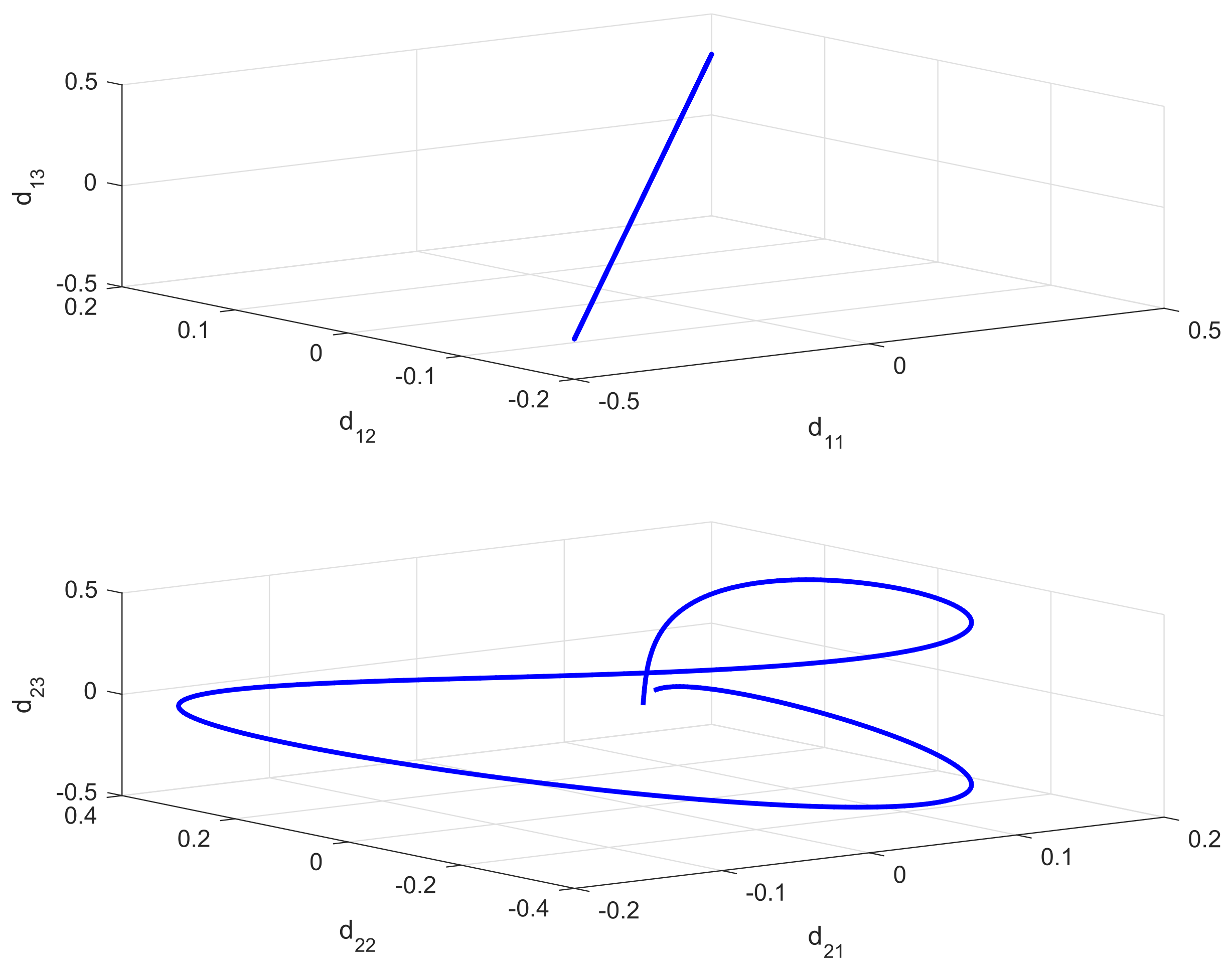
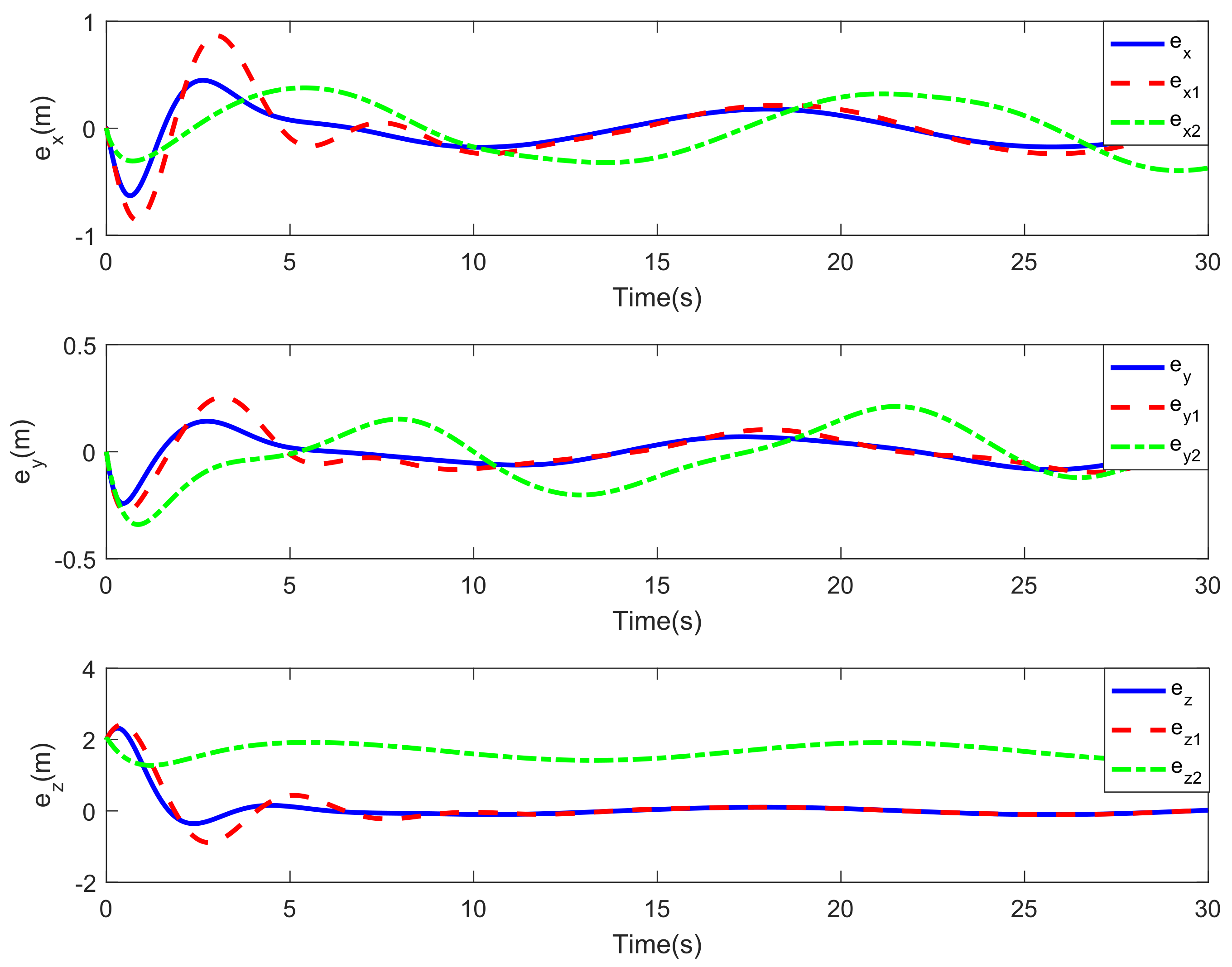
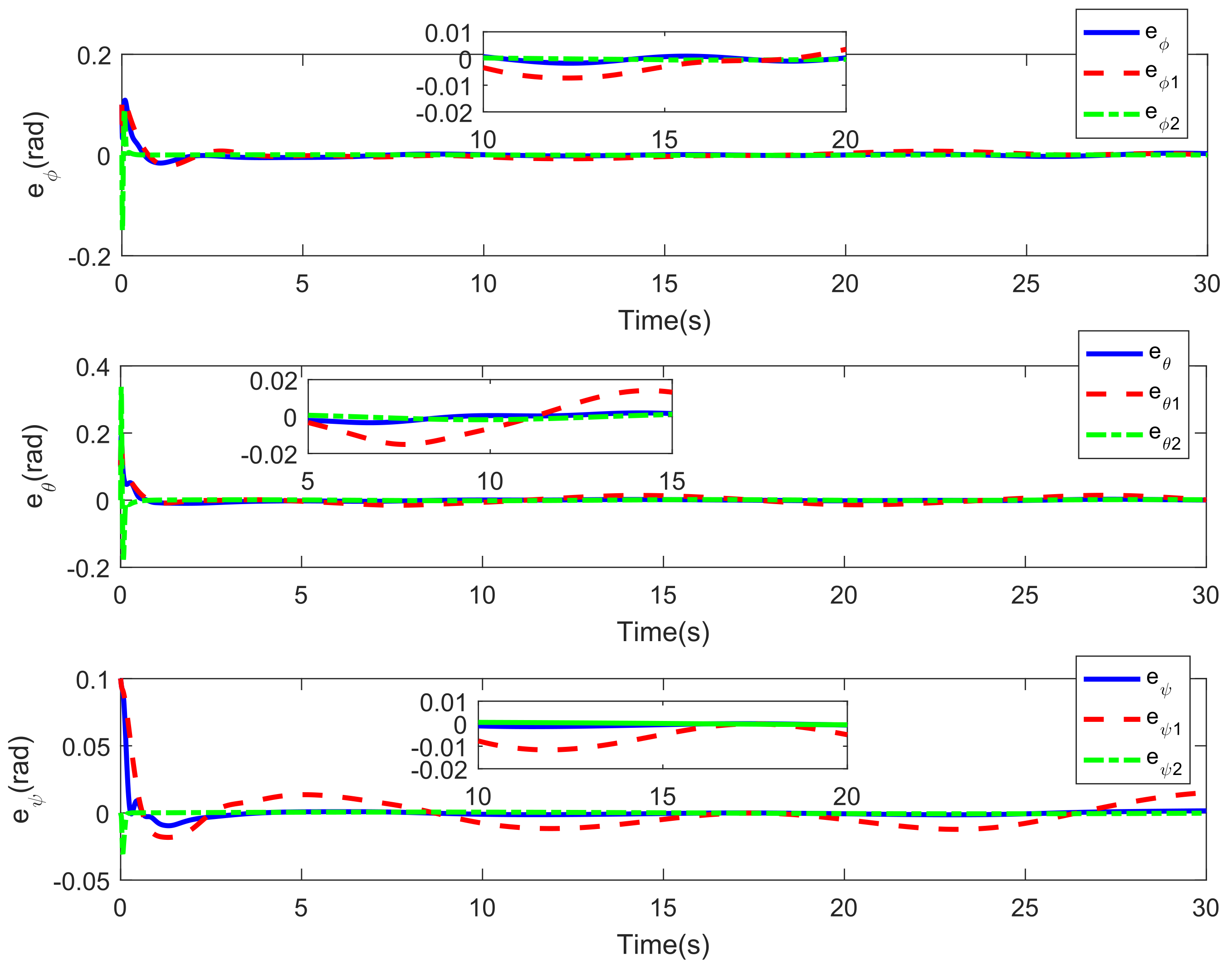
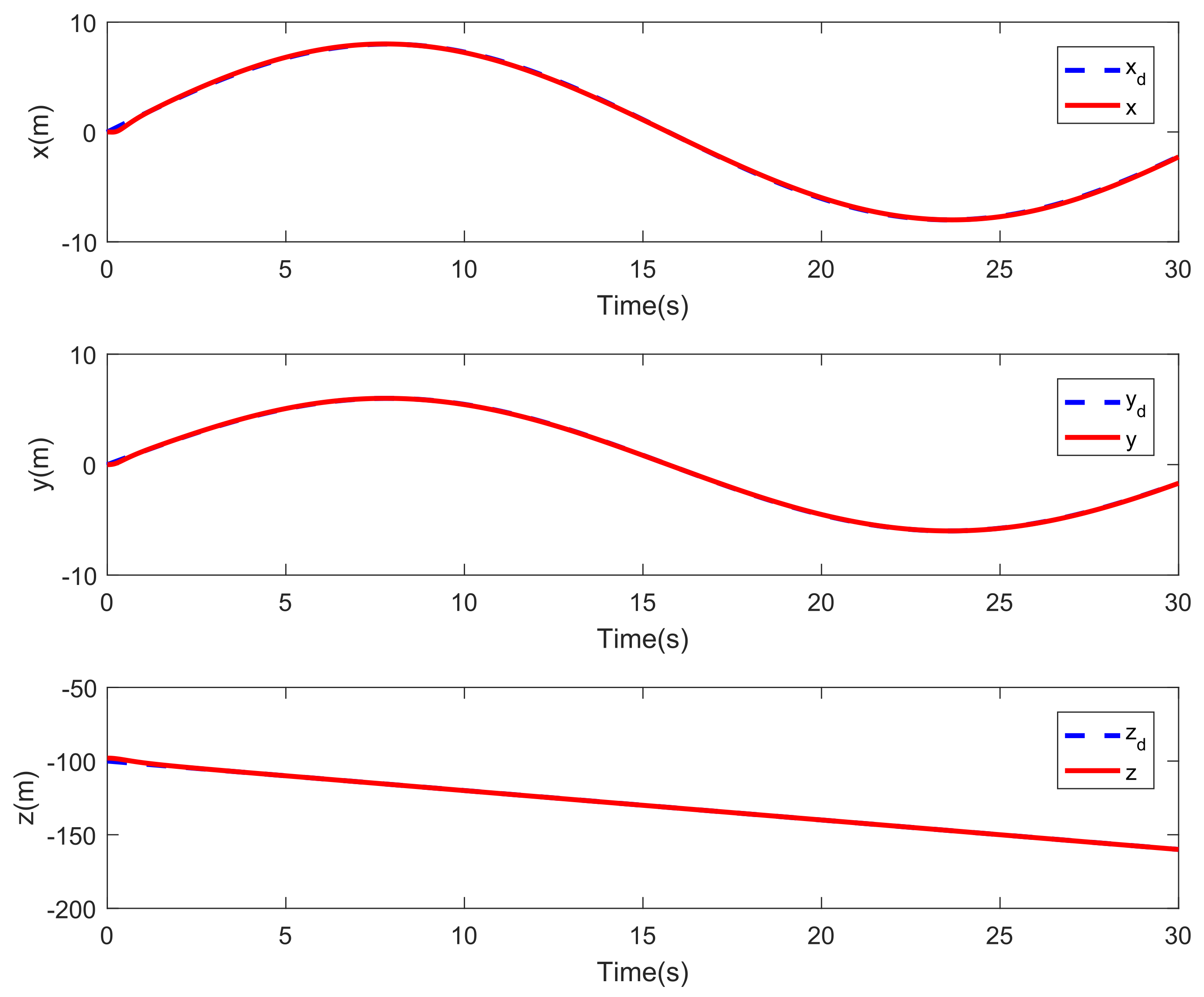
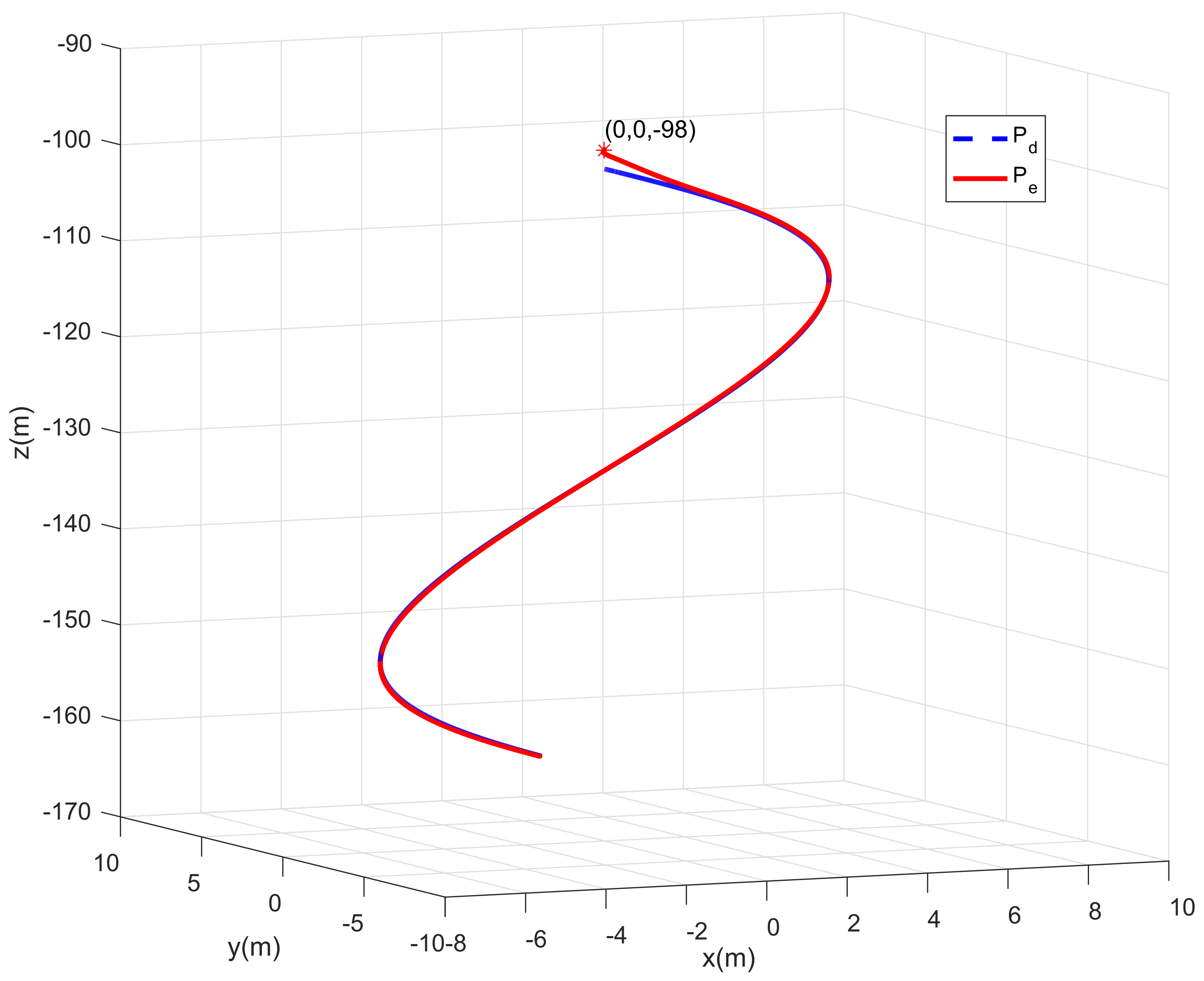
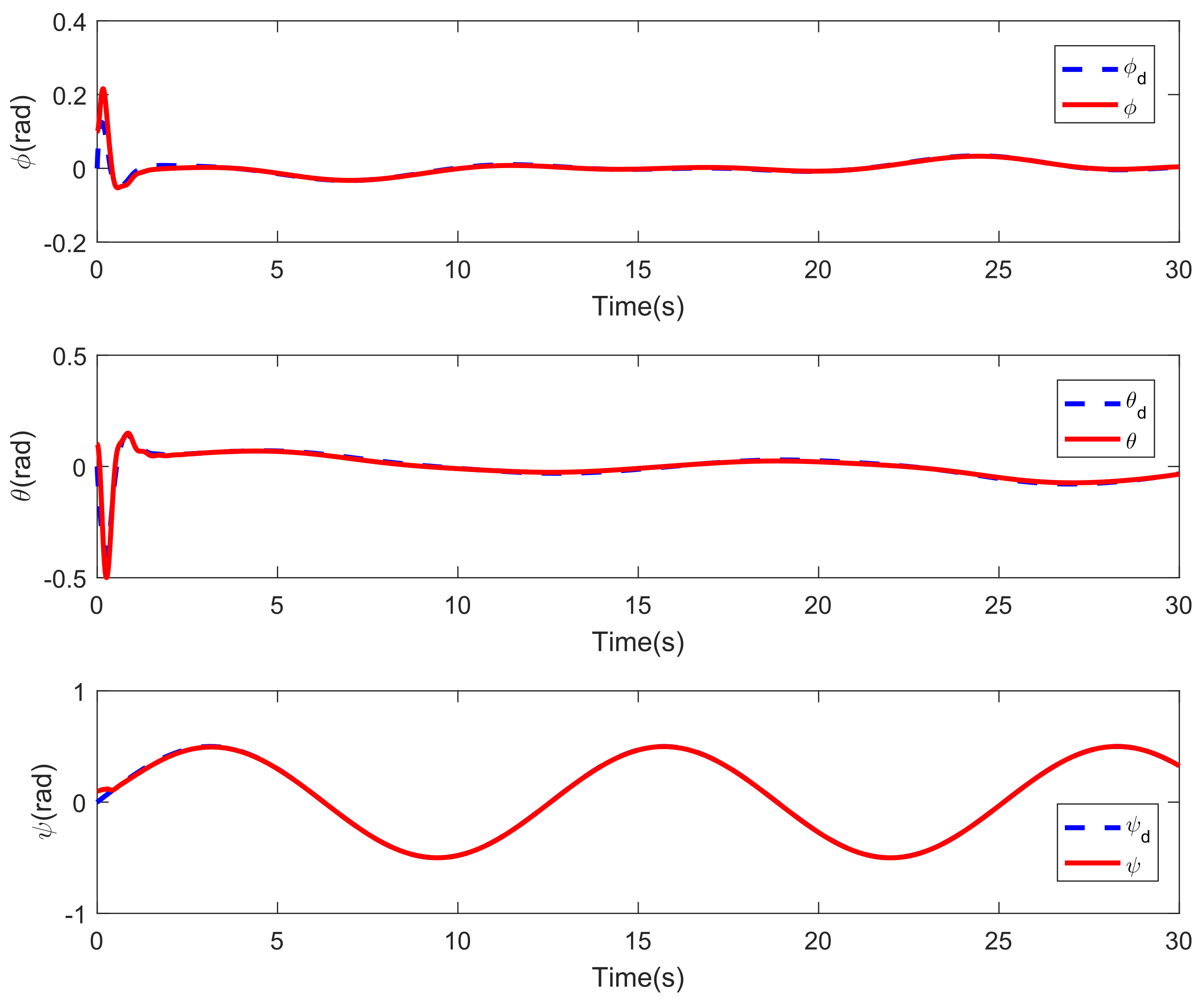
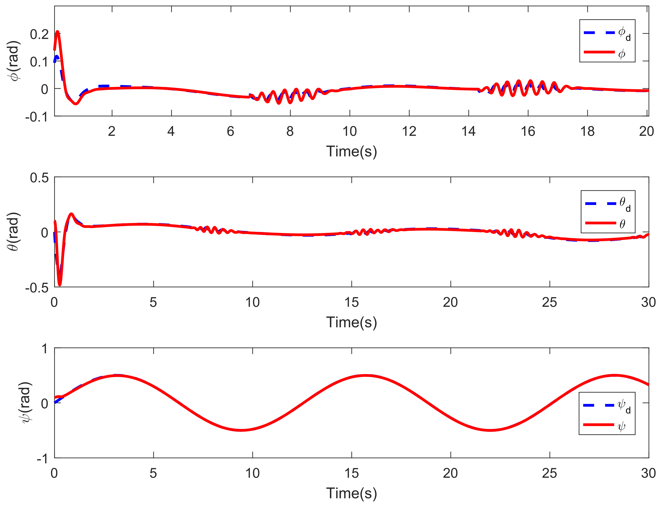
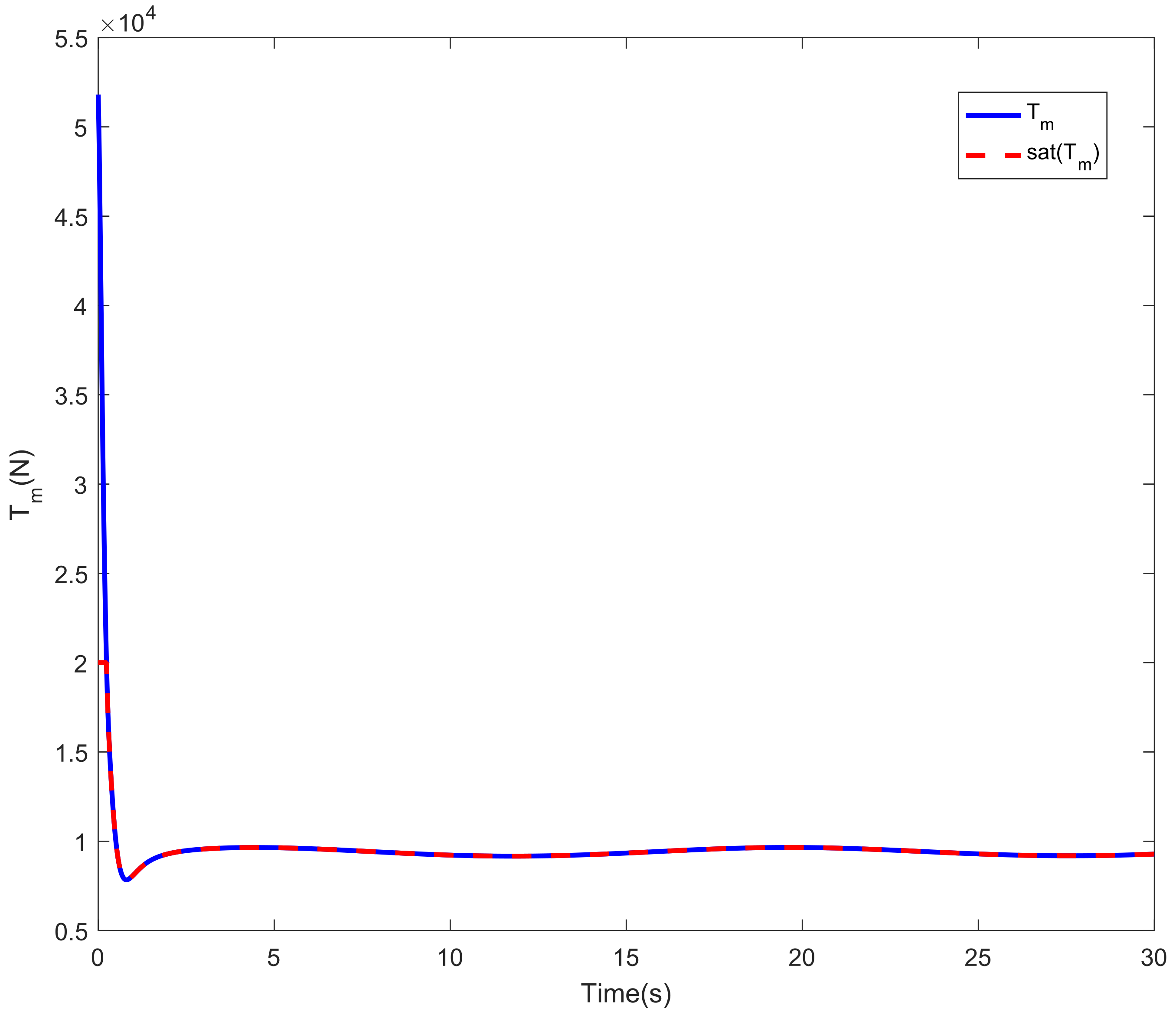
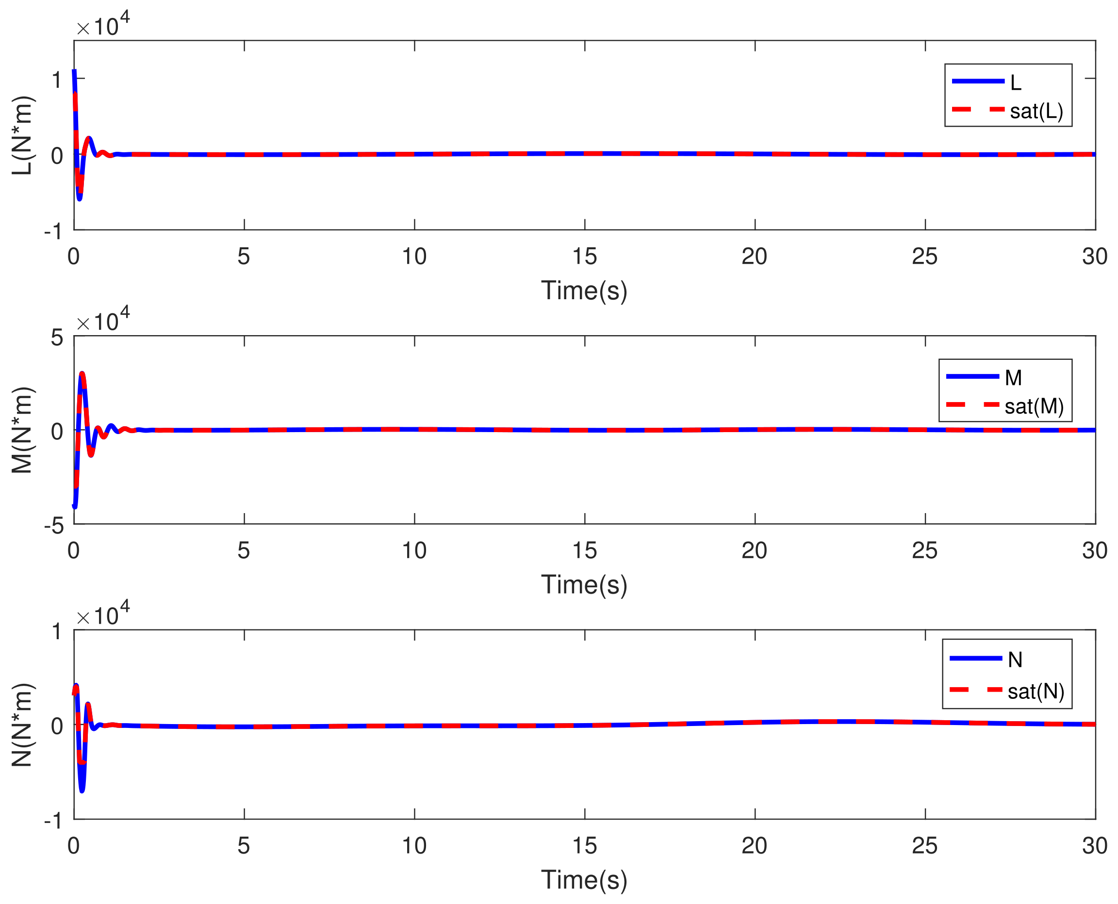
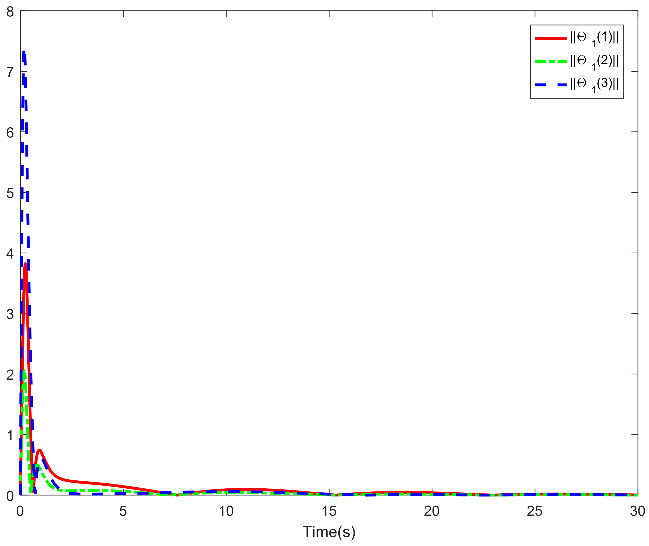
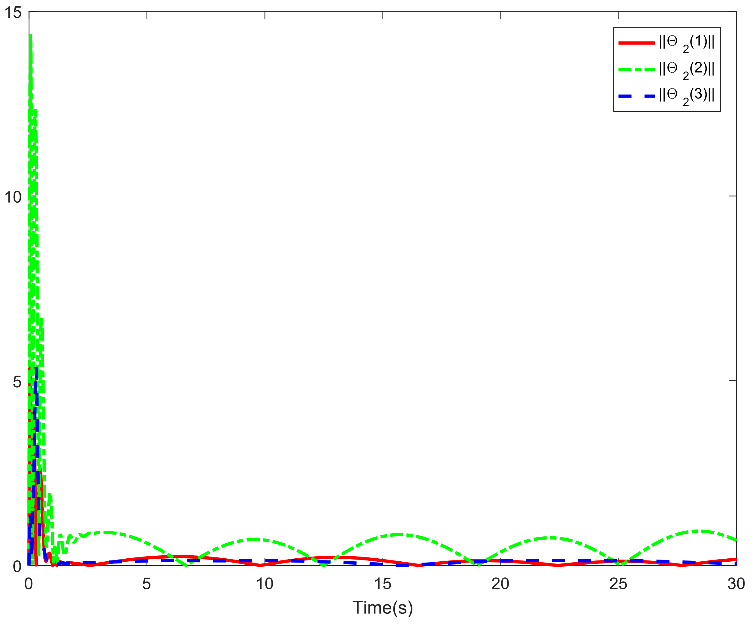
4. Simulation Results

Some simulations on the medium UAH are given to demonstrate the performance of the presented control scheme.

In this section, the physical properties related to the medium UAH are shown in

Table 1. Physical properties of the medium UAH.

Symbol	Definition	Value(unit)
m	Mass of UAH	800 kg
g	Acceleration of gravity	9.8 m/s2
$I_{xx}$	Moment of inertia along x axis	358.4 kg · m2
$I_{yy}$	Moment of inertia along y axis	777.9 kg · m2
$I_{zz}$	Moment of inertia along z axis	601.4 kg · m2

.

In this example, the initial states are assumed as $P_e(0)={[0,0,-98]}^{\mathrm{T}}(\mathrm{m})$, $\Lambda (0)={[0.1,0.1,0.1]}^{\mathrm{T}}(\mathrm{rad})$. Moreover, the tracking position trajectory is set as

$$P_d={[8sin(0.2t),6sin(0.2t),-100-2t]}^{\mathrm{T}}(\mathrm{m})$$

(63)

The expected attitude angle is set to ${\psi }_d=0.5sin(0.5t)(\mathrm{rad})$, and the remaining two angles are obtained by Formula (34).

Moreover, we consider the existence of system uncertainty and set it at 20%, while the external disturbances are chosen as

$$d_1={[0.5\ast sin(0.4t),0.2\ast sin(0.4t),0.3\ast sin(0.4t)]}^{\mathrm{T}},$$

$$d_2={[0.2\ast sin(0.3t),0.3\ast sin(0.5t),0.4\ast sin(0.2t)]}^{\mathrm{T}}.$$

where the 3D graphs of $d_1$ and $d_2$ are shown in Figure 2.

Remark 3. 

The premise of the proposed control method is that the performance of the UAH system is controllable in complex environments, such as uncertainty and bounded disturbances. If these conditions are not met (e.g., an unbounded disturbance (hurricane)), then the designed controller is invalid. When simulating external disturbances, we need to select the appropriate amplitude and frequency. They should not be too large, otherwise the UAH cannot provide the corresponding force and torque to achieve the control effect.

Furthermore, the relevant controller design parameters are, respectively, chosen as $K_1=\mathrm{diag}\{1,1,1\}$, $A_1=\mathrm{diag}\{0.1,0.1,0.1\}$, $K_3=\mathrm{diag}\{1,1,0.75\}$, $A_3=\mathrm{diag}\{2,3,2\}$, ${\eta }_1=0.8$, $T_1=\mathrm{diag}\{5,5,10\}$, ${\Gamma }_1=50$, ${\tau }_1=0.1$, ${\eta }_2=1$, $T_2=\mathrm{diag}\{10,10,10\}$, ${\Gamma }_2=50$, ${\tau }_2=0.1$, ${\kappa }_1={\kappa }_2={\kappa }_3={\kappa }_4=\mathrm{diag}\{10,10,10\}$, $r_1=r_3=\mathrm{diag}\{0.5,0.5,0.5\}$, $\gamma =\mathrm{diag}\{0.05,0.05,0.05\}$.

The backstepping SMC (green lines), the integral backstepping SMC without NN (red lines), and the proposed integral backstepping SMC combined with NN (blue lines) are selected, and their tracking effects are compared without considering input saturation. The tracking errors of the three controllers are shown in Figure 3 and Figure 4. Because the proposed control strategy combines the advantages of the backstepping SMC and NN, the tracking errors have shorter convergence times in the position and attitude angles, and the oscillation amplitude is smaller than that of other controllers.

Figure 5, Figure 6 and Figure 7 show the position and attitude-tracking response curves of the UAH system with the input saturation, disturbances, and uncertainty under the control scheme proposed in this paper. Figure 6 shows the 3D tracking renderings of the position. From Figure 5, it can be seen that trajectory tracking along the three axes is achieved. Figure 7 displays the tracking response curves of the three attitude angles. As can be observed from Figure 5, Figure 6 and Figure 7, the system can fast-track the expected signal without being affected by input saturation, uncertainty, and external disturbance.

We use attitude angle tracking as an example. It can be seen from Figure 8 that the sign function can generate chattering; replacing it with the tanh function can make the tracking effect smoother.

Figure 9 presents the control input of lift force and the control input with saturation in the position subsystem, while the control input of torques and the control input with saturation in the attitude subsystem are shown in Figure 10. The weights of the NN are shown in Figure 11 and Figure 12; the control effect shows that the NN can better compensate for the system uncertainty. To summarize, the proposed control design scheme has good robustness.

5. Conclusions

In this paper, a NN-based integral backstepping SMC scheme is proposed for a medium UAH subjected to input saturation, unknown system uncertainty, and disturbances. The auxiliary system was constructed to compensate for the adverse effects of input saturation. The unknown uncertainties were estimated by RBFNN; the estimation errors and the external disturbances were regarded as compound disturbances. The sliding mode controller was developed by the integral backstepping method to tackle the compound disturbances. The boundedness of the closed-loop system was guaranteed by the Lyapunov analysis. Finally, some numerical simulations confirmed that the controllers are effective and have good performance.

References

1. Yang, Y.D. Helicopter Flight Control, 3rd ed.; National Defense Industry Press: Beijing, China, 2007; pp. 32–70. [Google Scholar]
2. Yan, K.; Chen, M.; Wu, Q.; Jiang, B. Extended state observer-based sliding mode fault-tolerant control for unmanned autonomous helicopter with wind gusts. IET Control Theory Appl. 2019, 10, 1500–1513. [Google Scholar] [CrossRef]
3. Chaudhary, S.; Kumar, A. Control of Twin Rotor MIMO system using 1-degree-of-freedom PID, 2-degree-of-freedom PID and fractional order PID controller. In Proceedings of the 2019 3rd International conference on Electronics, Communication and Aerospace Technology (ICECA), Coimbatore, India, 12–14 June 2019; pp. 746–751. [Google Scholar]
4. Pounds, P.E.; Dollar, A.M. Stability of helicopters in compliant contact under PD-PID control. IEEE Trans. Robot. 2014, 30, 1472–1486. [Google Scholar] [CrossRef]
5. He, M.; He, J.; Scherer, S. Model-based real-time robust controller for a small helicopter. Mech. Syst. Signal Process. 2021, 14, 107022. [Google Scholar] [CrossRef]
6. Okyere, E.; Bousbaine, A.; Poyi, G.T.; Joseph, A.K.; Andrade, J.M. LQR controller design for quad-rotor helicopters. J. Eng. 2019, 17, 4003–4007. [Google Scholar] [CrossRef]
7. Mollov, L.; Kralev, J.; Slavov, T.; Petkov, P. μ-synthesis and hardware-in-the-loop simulation of miniature helicopter control system. J. Intell. Robot. Syst. 2014, 76, 315–351. [Google Scholar] [CrossRef]
8. Hu, Y.; Yang, Y.; Li, S.; Zhou, Y. Fuzzy controller design of micro-unmanned helicopter relying on improved genetic optimization algorithm. Aerosp. Sci. Technol. 2020, 98, 105685. [Google Scholar] [CrossRef]
9. Lee, J.; Seo, J.; Choi, J. Output feedback control design using Extended High-Gain Observers and dynamic inversion with projection for a small scaled helicopter. Automatica 2021, 133, 109883. [Google Scholar] [CrossRef]
10. Suprijono, H.; Kusumoputro, B. Direct inverse control based on neural network for unmanned small helicopter attitude and altitude control. J. Telecommun. Electron. Comput. 2017, 9, 99–102. [Google Scholar]
11. Mokhtari, A.; Msirdi, N.K.; Meghriche, K. Feedback linearization and linear observer for a quadrotor unmanned aerial vehicle. Adv. Robot. 2006, 20, 71–91. [Google Scholar] [CrossRef] [Green Version]
12. Aboudonia, A.; El-Badawy, A.; Rashad, R. Disturbance observer-based feedback linearization control of an unmanned quadrotor helicopter. Proc. Inst. Mech. Eng. Part I J. Syst. Control. Eng. 2016, 230, 877–891. [Google Scholar] [CrossRef]
13. Zhu, B.; Huo, W. Adaptive backstepping control for a miniature autonomous helicopter. In Proceedings of the 50th IEEE Conference on Decision and Control and European Control Conference, Orlando, FL, USA, 12–15 December 2011; pp. 5413–5418. [Google Scholar]
14. Sun, X.Y.; Fang, Y.C.; Sun, N. Backstepping-based adaptive attitude and height control of a small-scale unmanned helicopter. Control. Theory Appl. 2012, 29, 381–388. [Google Scholar]
15. Raptis, I.A.; Valavanis, K.P.; Moreno, W.A. A novel nonlinear backstepping controller design for helicopters using the rotation matrix. IEEE Trans. Control. Syst. Technol. 2011, 19, 465–473. [Google Scholar] [CrossRef]
16. Lee, C.T.; Tsai, C.C. Adaptive backstepping integral control of a small-scale helicopter for airdrop missions. Asian J. Control. 2010, 12, 531–541. [Google Scholar] [CrossRef]
17. Hamida, M.A.; Leon, J.D.; Glumineau, A. High-order sliding mode observers and integral backstepping sensorless control of IPMS motor. Int. J. Control. 2014, 87, 2176–2193. [Google Scholar] [CrossRef]
18. Poultney, A.; Gong, P.; Ashrafiuon, H. Integral backstepping control for trajectory and yaw motion tracking of quadrotors. Robotica 2019, 37, 300–320. [Google Scholar] [CrossRef]
19. Din, S.U.; Khan, Q.; Rehman, F.U.; Akmeliawanti, R. A comparative experimental study of robust sliding mode control strategies for underactuated systems. IEEE Access 2017, 5, 10068–10080. [Google Scholar] [CrossRef]
20. Lu, B.; Fang, Y.; Sun, N. Continuous sliding mode control strategy for a class of nonlinear underactuated systems. IEEE Trans. Autom. Control. 2018, 63, 3471–3478. [Google Scholar] [CrossRef]
21. Ullah, S.; Mehmood, A.; Khan, Q.; Rehman, S.; Iqbal, J. Robust integral sliding mode control design for stability enhancement of under-actuated quadcopter. Int. J. Control. Autom. Syst. 2020, 18, 1671–1678. [Google Scholar] [CrossRef]
22. Bessa, W.M.; Otto, S.; Kreuzer, E.; Seifried, R. An adaptive fuzzy sliding mode controller for uncertain underactuated mechanical systems. J. Vib. Control. 2019, 25, 1521–1535. [Google Scholar] [CrossRef]
23. Rsetam, K.; Cao, Z.; Man, Z. Design of robust terminal sliding mode control for underactuated flexible joint robot. IEEE Trans. Syst. Man Cybern. Syst. 2022, 52, 4272–4285. [Google Scholar] [CrossRef]
24. Zhang, M.; Zhang, Y.; Cheng, X. An enhanced coupling PD with sliding mode control method for underactuated double-pendulum overhead crane systems. Int. J. Control. Autom. Syst. 2019, 17, 1579–1588. [Google Scholar] [CrossRef]
25. Adhikary, N.; Mahanta, C. Integral backstepping sliding mode control for underactuated systems: Swing-up and stabilization of the Cart–Pendulum System. ISA Trans. 2013, 52, 870–880. [Google Scholar] [CrossRef]
26. Jia, Z.; Yu, J.; Mei, Y.; Chen, Y.; Shen, Y.; Ai, X. Integral backstepping sliding mode control for quadrotor helicopter under external uncertain disturbances. Aerosp. Sci. Technol. 2017, 68, 299–307. [Google Scholar] [CrossRef]
27. Nodland, D.; Zargarzadeh, H.; Jagannathan, S. Neural network-based optimal adaptive output feedback control of a helicopter UAV. IEEE Trans. Neural Netw. Learn. Syst. 2013, 24, 1061–1073. [Google Scholar] [CrossRef] [PubMed]
28. Li, L.; Zhang, H. Neural network based adaptive dynamic inversion flight control system design. In Proceedings of the 2011 2nd International Conference on Intelligent Control and Information Processing, Harbin, China, 25–28 July 2011; pp. 135–137. [Google Scholar]
29. Lee, T.; Kim, Y. Nonlinear adaptive flight control using backstepping and neural networks controller. J. Guidance Control Dyn. 2012, 24, 675–682. [Google Scholar] [CrossRef]
30. Mokhtari, S.; Abbaspour, A.; Yen, K.K.; Sargolzaei, A. Neural Network-Based Active Fault-Tolerant Control Design for Unmanned Helicopter with Additive Faults. Remote Sens. 2021, 13, 2396. [Google Scholar] [CrossRef]
31. Wang, D.; Zong, Q.; Tian, B.; Shao, S.; Zhang, X.; Zhao, X. Neural network disturbance observer-based distributed finite-time formation tracking control for multiple unmanned helicopters. ISA Trans. 2018, 73, 208–226. [Google Scholar] [CrossRef] [PubMed]
32. Ouyang, Y.; Dong, L.; Xue, L.; Sun, C. Adaptive control based on neural networks for an uncertain 2-DOF helicopter system with input deadzone and output constraints. IEEE/CAA J. Autom. Sin. 2019, 6, 807–815. [Google Scholar] [CrossRef]
33. Chen, M.; Ma, H.; Kang, Y.; Wu, Q. Adaptive neural safe tracking control design for a class of uncertain nonlinear systems with output constraints and disturbances. IEEE Trans. Cybern. 2021, 52, 12571–12582. [Google Scholar] [CrossRef] [PubMed]
34. Chen, M.; Tao, G.; Jiang, B. Dynamic surface control using neural networks for a class of uncertain nonlinear systems with input saturation. IEEE Trans. Neural Netw. Learn. Syst. 2015, 26, 2086–2097. [Google Scholar] [CrossRef] [PubMed]
35. Yang, Q.; Chen, M. Adaptive neural prescribed performance tracking control for near space vehicles with input nonlinearity. Neurocomputing 2016, 174, 780–789. [Google Scholar] [CrossRef]
36. Chen, M.; Yan, K.; Wu, Q. Multiapproximator-based fault-tolerant tracking control for unmanned autonomous helicopter with input saturation. IEEE Trans. Syst. Man Cybern. Syst. 2021, 52, 5710–5722. [Google Scholar] [CrossRef]
37. Wu, B.; Wu, J.; Zhang, J.; Tang, G.; Zhao, Z. Adaptive neural control of a 2DOF helicopter with input saturation and time-varying output constraint. Actuators 2022, 11, 336. [Google Scholar] [CrossRef]
38. Cai, G.; Chen, B.M.; Lee, T.H. Unmanned Rotorcraft Systems; Springer Science and Business Media: New York, NY, USA, 2011; pp. 97–128. [Google Scholar]
39. Chen, M.; Shi, P.; Lim, C. Adaptive neural fault-tolerant control of a 3-DOF model helicopter system. IEEE Trans. Syst. Man Cybern. Syst. 2016, 46, 260–270. [Google Scholar] [CrossRef] [Green Version]
40. Chen, M. Robust tracking control for self-balancing mobile robots using disturbance observer. IEEE/CAA J. Autom. Sin. 2017, 4, 458–465. [Google Scholar] [CrossRef]
41. Ge, S.S.; Wang, C. Adaptive neural control of uncertain MIMO nonlinear systems. IEEE Trans. Neural Netw. 2004, 15, 674–692. [Google Scholar] [CrossRef] [PubMed]
42. Chen, M.; Ge, S.S.; How, B.V.E. Robust adaptive neural network control for a class of uncertain MIMO nonlinear systems with input nonlinearities. IEEE Trans. Neural Netw. 2010, 21, 796–812. [Google Scholar] [CrossRef] [PubMed]
43. Wang, D.; Huang, J. Neural network-based adaptive dynamic surface control for a class of uncertain nonlinear systems in strict-feedback form. IEEE Trans. Neural Netw. 2005, 16, 195–202. [Google Scholar] [CrossRef]
44. Mokhtari, M.R.; Cherki, B.; Braham, A.C. Disturbance observer based hierarchical control of coaxial-rotor UAV. ISA Trans. 2017, 67, 466–475. [Google Scholar] [CrossRef]
Figure 1. Control design flow chart.
Drones 07 00154 g001
Figure 2. The 3D graphs of d 1 and d 2 .
Drones 07 00154 g002
Figure 3. Position tracking error comparison.
Drones 07 00154 g003
Figure 4. Attitude tracking error comparison.
Drones 07 00154 g004
Figure 5. Tracking response of the position.
Drones 07 00154 g005
Figure 6. The 3D graph of the position tracking.
Drones 07 00154 g006
Figure 7. Tracking response of the attitude.
Drones 07 00154 g007
Figure 8. Attitude tracking curve with the sign function.
Drones 07 00154 g008
Figure 9. Control force of the position subsystem.
Drones 07 00154 g009
Figure 10. Control torques of the attitude subsystem.
Drones 07 00154 g010
Figure 11. Norms of NN weight values, i.e., Θ 1 .
Drones 07 00154 g011
Figure 12. Norms of NN weight values, i.e., Θ 2 .
Drones 07 00154 g012