Abstract
In this paper, sensor fault diagnosis and fault tolerant control strategy are investigated for quadcopters under sensor faults and disturbances. We propose the fault diagnosis estimation system and the fault-tolerant control (FTC) method. The fault diagnosis system provides time-varying sensor fault estimation under an unknown bound of disturbances. Moreover, the fault-tolerant control eliminates disturbance that is estimated through the associated disturbance observer. Overall, the proposed FTC guarantees the finite-time tracking convergence using nonsingular fast terminal sliding mode algorithm. Stability of the closed-loop system is validated through the Lyapunov theory. Finally, conventional nonsingular fast terminal sliding mode and adaptive neural network sliding mode control are compared with the proposed method through simulations under sensor faults and disturbances with different scenarios.
1. Introduction
Over past decades, the topic of unmanned aerial vehicles (UAVs) has been studied widely because UAVs have promising applications in surveillance, rescue mission, entertainment, military, remote sensing, etc. With the development of mechanical and electronic technologies, different kinds of UAVs, such as fixed- and rotary-wing UAVs, have been developed in recent years to extend the application of UAVs. Quadcopter UAVs, one type of rotary-wing UAVs, have attracted special attention in industrial and academic field since they have simple structures yet superior maneuverability and agility at an affordable price.
To avoid quadcopter UAVs’ crashing during tracking, desired trajectory, and reliable attitude and position control systems are becoming more and more important. Many control system strategies have been suggested for quadcopters to track desired performance such as adaptive control [1,2], fuzzy logic control [3,4], gain scheduling [5,6], sliding mode control [7,8], proportional-integral-derivative control (PID) [9,10], and artificial intelligence method [11,12]. However, these methods did not consider faults in the quadcopter system. In case of actuator or sensor fault occurrence, these controllers cannot maintain normal operation for quadcopters. To overcome this problem, a fault-tolerant control (FTC) technique should be used. Normally, FTC techniques are categorized into two groups: active and passive schemes. The passive FTC (PFTC) scheme is designed as a robust controller to reduce fault effects. However, the active FTC (AFTC) scheme has been utilized for fault diagnosis and a fault accommodation approach to tolerate the faults. The AFTC scheme can provide better performance in the case of large faults. In this article, the AFTC scheme is investigated for the quadcopter system in the case of sensor fault occurrence. Accordingly, sensor fault diagnosis and fault tolerant control is examined.
Many research studies on fault diagnosis (FD) have been proposed for the quadcopter system. In [11,12], a robust fault diagnosis based on the Thau observer is presented for the quadcopter in the presence of an actuator fault. The results showed that a fault estimation algorithm can estimate the magnitude of a fault under model uncertainties. The fault detection and FD is proposed for a realistic non-linear UAV model [13]. The online fault parameter is estimated by dual Unscented Kalman filter (UKF). A two-stage Kalman filter algorithm is applied to estimate loss of control effectiveness in each actuator [14]. This work is validated through experiment with a quadrotor helicopter testbed. In [15], the magnitude of actuator fault is estimated through a parameter estimation scheme. Based on the fault estimation information, a nonlinear adaptive controller is suggested to guarantee the stability of the quadrotor system. In [16], a fault detection and isolation (FDI) based on a neural network in the case of an actuator fault is investigated. Some studies have shown promised results of an actuator fault diagnosis, but only few works focus on sensor diagnosis for quadrotor UAVs. In [17], an FDI and estimation method is presented for a quadrotor in the case of a gyroscope and accelerometer fault. In [18], a fault diagnosis strategy based on the Thau observer and Lipschitz nonlinear model is presented for a quadrotor considering actuator and sensor faults. An FDI scheme with various kinds of sensor faults is examined in [19]. The nonlinear identity observer is suggested to detect faults, and the generalized observer scheme is used to isolate the sensor faults. A sensor fault diagnosis of a quadrotor UAV based on a two-stage Kalman filter algorithm is considered in [20]. In [21], a robust sensor fault detection algorithm based on performance is proposed for the quadrotor. The suggested strategy can show a good tracking performance under sensor faults and external disturbances. In the latest article [22], a fault-tolerant control based on command filter backstepping and dynamic control allocation is proposed for drone interceptors with fixed wings and reaction jets in the presence of actuator faults. This control method consists of two parts: nonlinear virtual control strategy and dynamic control allocation. Although the virtual control law is designed to handle system uncertainties, the fault-weighing dynamic control allocation is suggested to distribute the control signal for each actuator. The results show that the proposed method can track quickly and smoothly acceleration commands under actuator faults. Although a fault diagnosis algorithm is crucial, it is insufficient to guarantee the normal operation of the quadrotor UAVs. Fault diagnosis is not the ultimate goal in the control of a quadcopter system, whereas safety and reliability during operation is a key feature. This means that the control system needs to be designed to maintain stability, quality, and normal operation in the presence of faults [23]. This requires the emergence of FTC systems.
In terms of FTC for quadcopter UAVs, most current studies emphasize actuator faults [24,25,26,27]. Few research papers focus on the sensor FTC system in comparison with the actuator FTC system. In [28], an attitude fault-tolerant control scheme is proposed for the quadcopter in the presence of sensor faults. The attitude is estimated using an array of nonlinear observer information. The observer information is applied to compensate the amount of sensor faults. However, this method does not consider external disturbance in quadrotor modeling. In [29], active fault-tolerant control is suggested for the quadrotor under a sensor fault. Fault diagnosis based on the observer is designed to estimate the magnitude of sensor fault. Then, this sensor fault estimation is integrated into PID control for sensor fault compensation. However, the suggested fault diagnosis only considers the model of the global positioning system (GPS) fault, which is not a general case. Moreover, the FTC control technique based on PID is insufficient to handle the disturbances and model uncertainties.
In the study [30], robust tracking control and a fault detection algorithm is proposed for the UAV. The suggested fault diagnosis can detect and isolate faults through residual evaluations, but it cannot estimate the magnitude of faults which can integrate with the designed controller for fault accommodation. In [31], sensor fault diagnosis based on residual evaluation is presented to detect fault. After the fault is detected, a redundant sensor is used for compensation. This method can provide a good strategy for real application in the presence of the failure in the altitude sensor, but it is expensive when considering all navigation sensors. In a recent article [32], a fault-tolerant control based on a sliding mode and a neural network is proposed in the presence of an actuator and sensor fault. This work used an adaption law through gradient descent method to tune the parameters in radial basis function (RBF) neural networks. The results show that the controller can handle actuator and sensor faults. A sensor fault-tolerant control based on a nonlinear Kalman filter is proposed in [33]. When all filters exceed the threshold values, a sensor bias term is measured and added to the state values of the system. However, this method does not consider external disturbance in the system model. Moreover, using a PID controller is not enough to handle the nonlinear term of the system model. An active disturbance rejection-based fault-tolerant control is presented in [34] to handle sensor faults and disturbance, but the fault-tolerant control based on a proportional derivative controller is insufficient to handle sudden faults or time-varying faults. To date, the development of sensor fault diagnosis and tolerant control for quadcopter UAVs as a complete unit has not been studied intensively. Furthermore, most of the above-mentioned studies did not extensively discuss the finite-time convergence for the quadrotor system in the presence of both sensor faults and disturbances.
To overcome the above limitations for improving the robustness of control performance, this article presents a sliding mode observer-based fault diagnosis, and finite-time FTC scheme for quadrotor UAVs against both sensor faults and disturbances. Major contributions of this research work can be summarized as follows:
- ✓
- We develop a fault diagnosis and FTC system based on a sliding mode observer, a disturbance observer, and a nonsingular fast terminal sliding mode to handle external disturbances and sensor faults.
- ✓
- Stability of the closed-loop system is proved using the Lyapunov theory and the proposed method is compared with existing algorithms.
- ✓
- Unlike previous studies on fault diagnosis algorithm, the proposed fault diagnosis system can estimate the magnitude of sensor faults under an unknown bound of external disturbances.
- ✓
- Unlike most current research papers, the proposed method guarantees that the control system converges in a finite time with small steady-state errors.
The rest of this paper is organized as follows. The mathematical model of the quadrotor is presented in Section 2. Then, the proposed fault diagnosis and FTC scheme are described in Section 3 and Section 4. Simulation results are shown in Section 5 to validate the effectiveness of the proposed scheme. General conclusions of this paper are summarized in Section 6.
2. Mathematical Model of Quadcopter
The quadcopter configuration referred in this paper is depicted in Figure 1. Four motors are mounted in a plus configuration. Motor 1 and 3 rotate clockwise, while the other two motors spin counterclockwise. Forces induced by the motors are denoted as , and angular velocities as . The earth and body frames are presented in Figure 1 respectively as , and .
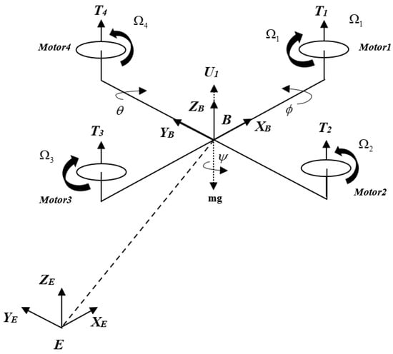
Figure 1.
Quadcopter model.
As shown in Figure 1, the total thrust in the -direction is described as:
where is the thrust coefficient.
The control torques in the , , direction are denoted by as follow:
where denotes as arm length which is the distance between the center of the quadcopter to each motor, and is drag coefficient.
The relationship between the control input and output is expressed as:
According to the Newton–Euler law, the altitude and attitude of the quadcopter system can be expressed as:
where is the gravity constant, denotes the total mass of the quadcopter, , and represent inertia moments. The global position of the quadcopter is denoted as . Damping terms are represented as . The roll, pitch, and yaw angles are denoted as , and , respectively. Disturbances are denoted as .
Let us define the state vector as:
General model of the quadcopter under an actuator fault may be expressed as:
where denotes each subsystem:
3. Fault Diagnosis Scheme for Quadcopter
From Equation (7), the state-space model of the sensor fault in the attitude system can be expressed by:
where are the state, input, and output vector respectively; is the sensor fault vector; the disturbance term denotes as , . Matrices are chosen as:
From Equations (4) and (7), we can see that disturbance terms affect mainly the second derivative of roll, pitch, and yaw. Therefore, the matrix is considered as shown in Equation (9).
We assume that attitude angles are prone to fault during the flight test. Therefore, the first three states of faulty matrix are nonzero such that the Assumption 5 [35] (presented in the next section) is satisfied. Similarly, if we consider the fault of angular velocity, the last three terms of matrix are nonzero, and the first three terms are zero. In this article, we only use three states for fault diagnosis. It is not possible to use six states due to the Assumption 5 and reference [35], which is limitation of current works.
Denote . The augmented system can be described as:
where .
Development of the fault diagnosis scheme is based on several assumptions and lemmas stated here.
Assumption 1.
is observable.
Assumption 2.
There exists an unknown M such that the disturbance term is norm-bounded.
Assumption 3.
([35,36]) is differentiable after their occurrence.
Assumption 4.
Nonlinear vector function
in Equation (8) is a continuously differentiable and assumed to be locally Lipschitz with constant
, i.e.,
.
Assumption 5.
([35]) The matrix has full column rank with
Lemma 1.
([29]) Given a scalar and a symmetric positive definite matrix
, then the following inequality holds:
Lemma 2.
[30] If a positive-definite function, , satisfies
with
and
, can be defined as the fast-finite-time stability, and
is the settling time required to reach
,
. The adaptive fault diagnosis observer model is constructed as:
where , , is the state observer vector, output vector, and observer gain, is chosen such that is a stable matrix, with the gain updated by
where is the positive gain and is a small positive number.
Let us define:
Dynamics of estimation error is described by:
Remark 1.
After several iterations, then the uncertain term
is separated from the estimation error (15). Therefore, we can estimate these disturbances. The suitable choice of matrix
and positive scalar
can eliminate the term
but the first derivative of
still remains on the expression of. Two purposes are examined to design observer (4) as follows:
A1. The estimation error is asymptotically stable if .
A2. For all nonzero , the performance index function is defined by:
where denotes a positive scalar, then the following theorem is considered.
Theorem 1.
Let Assumption 1–4 hold. If there exists a symmetric positive definite matrixwith given positive constants
such that the following conditions holds:
where with , then the state and fault estimation error are asymptotically stable.
Proof of Theorem 1.
The Lyapunov function is selected as
The first derivative of is achieved by:
According to (17) and positive definite matrix in Theorem 1, one gets:
From Assumption 4, Lemma 1, and Equation (14), one achieves [36]:
Insert Equations (20) and (21) to (19), one obtains:
The performance index function is chosen to ensure that the adaptive observer is robust against the external disturbance as
With the initial conditions , we obtain:
where and is the minimum eigenvalue of the matrix.
From Theorem 1, one can see that the term holds, thus:
We conclude from Equation (18) that the state and fault estimation error are asymptotically stable such that:
This completes the proof. □
Remark 2.
The adaptation law (13) is developed based on the quadratic Lyapunov function (18). As discussed in [37,38], non-quadratic Lyapunov functions usually lead to a better performance in adaptive algorithms.
4. Fault-Tolerant Control with Disturbance Observer
This section first introduces the design of disturbance observer. Then, the nonsingular fast terminal sliding mode surface and the control law are designed and integrated with the observer.
4.1. Disturbance Observer Design
Assumption 6.
The disturbancein system (6) is norm bounded as:
where
is a known constant.
To estimate the disturbance , a nonlinear disturbance observer is obtained as
where is the auxiliary variable of nonlinear observer; and are the observer gains.
Theorem 2.
Consider the quadcopter system model (6) with the disturbance observer defined by (28). If the Lyapunov function is chosen as Equation (29), then can estimate precisely. Thus, after finite time.
Proof of Theorem 2.
The Lyapunov function is selected as:
The first derivative of Lyapunov function is:
where
From Lemma 2, Equation (30) implies that converges to the equilibrium in finite time.
The disturbance error is calculated as:
From the conclusion of Equation (30), we can obtain . □
4.2. Integrate Nonsingular Fast Terminal Sliding Mode Control with Disturbance Observer
The sliding surface for the quadcopter system can be expressed as:
where .
The derivative of the sliding surface is:
Theorem 3.
Consider the system (6) and the sliding surface (33), recall the estimated attitude sensor faults and disturbances observer, if the control law is designed as:
where, and the Lyapunov function designed as Equation (35), then the tracking error converges to equilibrium within finite time.
Proof.
Choosing the Lyapunov function as
Recall sensor fault estimation in Section 3, the derivative of the Lyapunov function is achieved through Equation (34) as:
From Equation (31), one obtains:
where , .
Therefore, the stability of the proposed controller can be guaranteed with the suggested control law (34) in the presence of disturbances. □
Remark 3.
In the control law (34), the term is defined through Equation (6). Assume the attitude angles are limited within the range as:, then the term
is nonzero vector because the inertia moment values () are nonzero.
Remark 4.
The fault diagnosis system based on observer method in Equation (12) and fault tolerant control algorithm in Equation (34) are not complex. These methods do not require high computation for an embedded system, which is feasible to implement on a real quadcopter system.
5. Simulations
The proposed FTC method is compared with an adaptive neural sliding mode control (ANNSMC) [33] and a conventional nonsingular fast terminal sliding mode control (NSFTSMC) [39] in this section. The parameters of quadcopter DJI F330 [40] are chosen as . Equations (16) and (17) of the fault diagnosis system is solved using the linear matrix inequality (LMI) toolbox as
The positive gain in Equation (13) is chosen as , while the parameters of FTC in Equation (34) are selected as follows:. They are selected by trial and error.
Four scenarios are set up to show effectiveness of the proposed methods. The first scenario investigates the proposed fault diagnosis algorithm, whereas the remaining scenarios examine the suggested FTC strategies.
5.1. Fault Diagnosis Test
To show the effectiveness of the proposed fault diagnosis, constant and time-varying sensor faults are injected into the roll, pitch, and yaw angles as follow:
The time-varying disturbances are chosen as . It can be seen from Figure 2 that while faults occur in attitude measurements starting from , the estimated values converge to actual fault values quickly. Hence, the proposed fault diagnosis algorithm can estimate the fault signals accurately under time-varying disturbances. The estimation of fault diagnosis will be used in the FTC system.
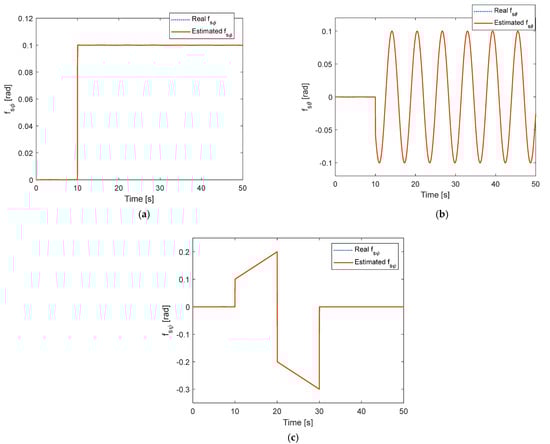
Figure 2.
Sensor fault estimation under time-varying disturbance: (a) For roll angle; (b) For pitch angle; (c) For yaw angle.
5.2. Fault Tolerant Control Test
Three scenarios are set up to show the effectiveness of the proposed FTC system. Firstly, the constant sensor faults are injected into the quadcopter system as at without considering the disturbances of the quadcopter model. The results of attitude are shown in Figure 3. It is seen that the roll, pitch, and yaw from conventional NSFTSMC and ANNSMC cannot converge to desired values. On the contrary, the proposed FTC method provides a good tracking performance. Commanded roll, pitch, and yaw can be tracked again after the faults have occurred. Estimation of constant sensor faults is depicted in Figure 4. Fault estimation from the fault diagnosis algorithm in Section 3 converges accurately to the desired value of 0.02 in roll, pitch, and yaw angles.
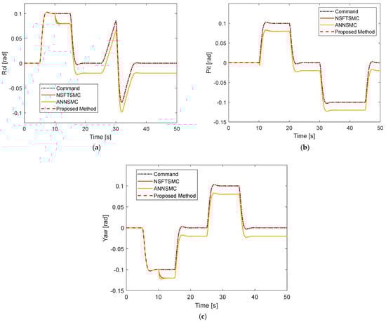
Figure 3.
Tracking performance under constant fault without disturbance: (a) Roll motion; (b) Pitch motion; (c) Yaw motion.
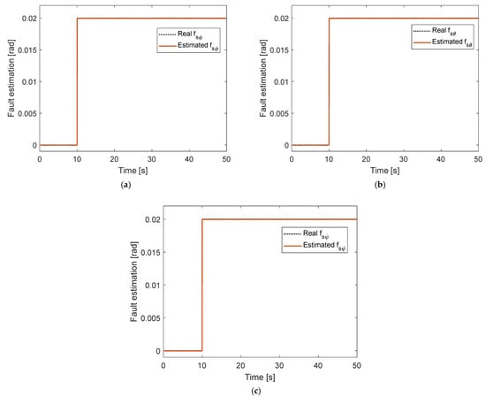
Figure 4.
Fault estimation under constant fault without disturbance: (a) In roll motion; (b) In pitch motion; (c) in yaw motion.
In the second scenario, constant faults of the first scenario are still employed. However, time-varying disturbances of are injected to roll, pitch, and yaw motion. The tracking performance of the roll, pitch, and yaw angles is presented in Figure 5. Under time-varying disturbance, the attitude performance of conventional NSFTSMC has oscillations and deviations during tracking performance, while that of ANNSMC shows deviations from the desired position. Neither method could track the desired value well. On the other hand, the proposed method provides good tracking performance under constant fault and time-varying disturbance. Corresponding fault estimation and disturbance estimation in roll, pitch, and yaw are shown in Figure 6 and Figure 7. Both estimations converge quickly to the actual values, yielding good tracking performance.
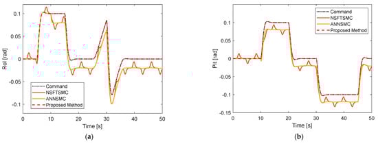
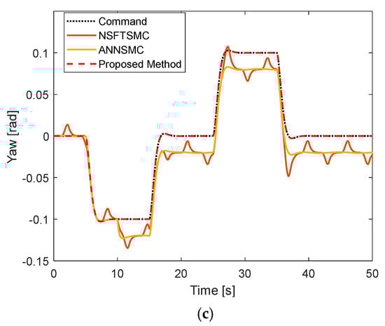
Figure 5.
Track performance under constant sensor fault and time-varying disturbance: (a) In Roll motion; (b) In Pitch motion; (c) In yaw motion.
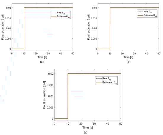
Figure 6.
Fault estimation under constant fault and time-varying disturbance: (a) Roll motion; (b) Pitch motion; (c) Yaw motion.
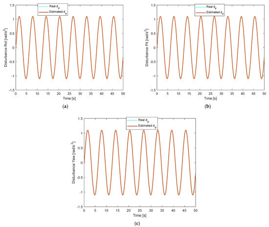
Figure 7.
Disturbance estimation under constant fault and time-varying disturbance: (a) In Roll motion; (b) In Pitch motion; (c) In Yaw motion.
Integral square error (ISE) performance index can be used to quantitatively compare among NSFTSMC, ANNSMC, and proposed FTC methods:
where and are the initial and final instants, and the tracking error. From two scenarios above, the results can be concluded in Table 1 and Table 2. It is apparent that the proposed method, which yields accurate tracking and fewer errors in the presence of sensor faults and time-varying disturbances, is superior to the NSFTSMC and ANNSMC control approaches.

Table 1.
ISE performance indexes for constant faults.
Table 2.
ISE performance indexes for constant faults and disturbances.
In the previous two scenarios, the proposed method has a better performance compared to other techniques. To show the robustness of the proposed method under both time-varying faults and time-varying disturbances, the time-varying faults are injected to roll, pitch, and yaw angle as:
with the same time-varying disturbances as in the second scenario. Attitude performance is depicted in Figure 8. The proposed FTC algorithm can track desired roll, pitch, and yaw angles accurately. Sensor fault estimation is shown in Figure 9. The proposed fault diagnosis algorithm quickly converges to actual values of roll, pitch, and yaw angles.
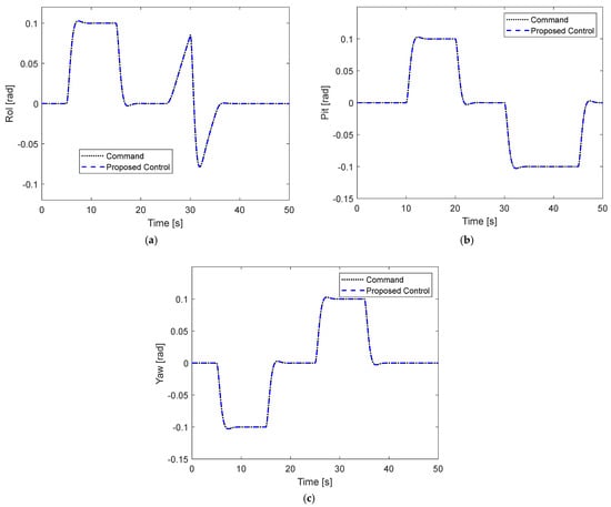
Figure 8.
Tracking performance under time-varying sensor fault and time-varying disturbance: (a) In Roll motion; (b) In Pitch motion; (c) In Yaw motion.
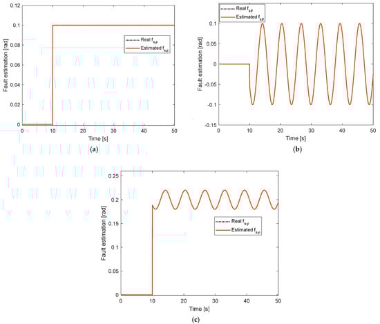
Figure 9.
Fault estimation under time-varying sensor fault and time-varying disturbance: (a) In Roll angle; (b) In Pitch angle; (c) In Yaw angle.
Remark 5.
For testing the suggested algorithm on a quadcopter system, an outdoor environment can be applied for flight tests. The essential hardware and software, such as a mission planner using a ground control system, and a flight controller are utilized during trials. The status of a drone can be achieved by receivers (known as telemetry). Navigation of the quadcopter is accomplished by sending the attitude and altitude commands.
6. Conclusions
This paper presents fault diagnosis and a fault-tolerant control algorithm for quadcopters to handle sensor faults and disturbances. The suggested fault diagnosis system can estimate sensor fault under an unknown upper bound of disturbance. This estimation information is then applied to the fault-tolerant control system. In terms of the proposed FTC, it can estimate the magnitude of disturbance, which avoids the burden of the high gain from the fault-tolerant control system. Compared with conventional nonsingular fast terminal sliding mode control and adaptive neural network sliding mode control, our approach demonstrates fast tracking, fewer errors, and superior robustness under various fault and disturbance conditions. In this paper, only IMU sensor faults are considered, but sensor noise, angular velocity, GPS and actuator faults are also important and not discussed intensively so far, which is the limitation of this paper. We plan to apply the proposed fault diagnosis and fault-tolerant control system to the real UAV. It is expected to enhance the reliability and stability during flight tests under hazardous environments. Moreover, artificial intelligence-based fault-tolerant control will be investigated to handle the actuator, IMU, GPS faults, and sensor noise as a complete unit.
Author Contributions
Conceptualization, N.-P.N. and P.P.; methodology, N.-P.N. and P.P.; software, N.-P.N.; validation, N.-P.N.; formal analysis, N.-P.N. and P.P.; investigation, N.-P.N. and P.P.; resources, P.P.; data curation, N.-P.N. and P.P.; writing—original draft preparation, N.-P.N.; writing—review and editing, N.-P.N. and P.P.; visualization, N.-P.N.; supervision, P.P.; project administration, P.P.; funding acquisition, P.P. All authors have read and agreed to the published version of the manuscript.
Funding
This research project is supported by the Second Century Fund (C2F), Chulalongkorn University.
Data Availability Statement
Not applicable.
Acknowledgments
The authors gratefully acknowledge generous support from the Second Century Fund (C2F), Chulalongkorn University.
Conflicts of Interest
The authors declare no conflict of interest.
References
- Zhou, L.; Xu, S.; Jin, H.; Jian, H. A hybrid robust adaptive control for a quadrotor UAV via mass observer and robust controller. Adv. Mech. Eng. 2021, 13, 16878140211002723. [Google Scholar] [CrossRef]
- Wu, Y.; Xie, Y.; Li, S. Parameter Adaptive Control for a Quadrotor with a Suspended Unknown Payload under External Disturbance. IEEE Access 2021, 9, 139958–139967. [Google Scholar] [CrossRef]
- Zhou, Y.; Kumar, A.; Parkash, C.; Vashishtha, G.; Tang, H.; Glowacs, A.; Dong, A.; Xiang, J. Development of entropy measure for selecting highly sensitive WPT band to identify defective components of an axial piston pump. Appl. Acoust. 2023, 203, 109225. [Google Scholar] [CrossRef]
- Lara Alabazares, D.; Rabhi, A.; Pegard, C.; Torres Garcia, F.; Romero Galvan, G. Quadrotor UAV attitude stabilization using fuzzy robust control. Trans. Inst. Meas. Control 2021, 43, 2599–2614. [Google Scholar] [CrossRef]
- Melo, A.G.; Andrade, F.A.A.; Guedes, I.P.; Carvalho, G.F.; Zachi, A.R.L.; Pinto, M.F. Fuzzy Gain-Scheduling PID for UAV Position and Altitude Controllers. Sensors 2022, 22, 2173. [Google Scholar] [CrossRef]
- Derrouaoui, S.H.; Bouzid, Y.; Guiatni, M. PSO Based Optimal Gain Scheduling Backstepping Flight Controller Design for a Transformable Quadrotor. J. Intell. Robot. Syst. Theory Appl. 2021, 102, 67. [Google Scholar] [CrossRef]
- Nekoukar, V.; Mahdian Dehkordi, N. Robust path tracking of a quadrotor using adaptive fuzzy terminal sliding mode control. Control Eng. Pract. 2020, 110, 104763. [Google Scholar] [CrossRef]
- Ghadiri, H.; Emami, M.; Khodadadi, H. Adaptive super-twisting non-singular terminal sliding mode control for tracking of quadrotor with bounded disturbances. Aerosp. Sci. Technol. 2021, 112, 106616. [Google Scholar] [CrossRef]
- Wang, S.; Polyakov, A.; Zheng, G. Quadrotor stabilization under time and space constraints using implicit PID controller. J. Frankl. Inst. 2022, 359, 1505–1530. [Google Scholar] [CrossRef]
- Gautam, D.; Ha, C. Control of a quadrotor using a smart self-tuning fuzzy PID controller. Int. J. Adv. Robot. Syst. 2013, 10, 380. [Google Scholar] [CrossRef]
- Cen, Z.; Noura, H.; Susilo, T.B.; Al Younes, Y. Robust Fault Diagnosis for quadrotor uavs using Adaptive Thau observer. J. Intell. Robot. Syst. Theory Appl. 2014, 73, 573–588. [Google Scholar] [CrossRef]
- Cen, Z.; Noura, H.; Younes, Y.A. Systematic fault tolerant control based on adaptive Thau observer estimation for quadrotor UAVs. Int. J. Appl. Math. Comput. Sci. 2015, 25, 159–174. [Google Scholar] [CrossRef]
- Ma, L.; Zhang, Y. Fault Detection and Diagnosis for GTM UAV with dual Unscented Kalman Filter. In Proceedings of the AIAA Guidance, Navigation, and Control Conference, Toronto, ON, Canada, 2–5 August 2010. [Google Scholar]
- Amoozgar, M.H.; Chamseddine, A.; Zhang, Y. Experimental test of a two-stage kalman filter for actuator fault detection and diagnosis of an unmanned quadrotor helicopter. J. Intell. Robot. Syst. Theory Appl. 2013, 70, 107–117. [Google Scholar] [CrossRef]
- Ranjbaran, M.; Khorasani, K. Generalized fault recovery of an under-actuated quadrotor aerial vehicle. In Proceedings of the 2012 American Control Conference (ACC), Montreal, QC, Canada, 27–29 June 2012. [Google Scholar]
- Abbaspour, A.; Yen, K.K.; Forouzannezhad, P.; Sargolzaei, A. A Neural Adaptive Approach for Active Fault-Tolerant Control Design in UAV. IEEE Trans. Syst. Man Cybern. Syst. 2020, 50, 3401–3411. [Google Scholar] [CrossRef]
- Avram, R.C.; Zhang, X.; Campbell, J.; Muse, J. IMU sensor fault diagnosis and estimation for quadrotor UAVs. IFAC-PapersOnLine 2015, 28, 380–385. [Google Scholar] [CrossRef]
- Zhong, Y.; Zhang, Y.; Zhang, W.; Zhan, H. Actuator and sensor fault detection and fault diagnosis for unmanned quadrotor helicopters. IFAC PapersOnline 2018, 51, 998–1003. [Google Scholar] [CrossRef]
- Noura, H.; Rabhi, A. Sensor fault detection and isolation in quadrotor vehicle using nonlinear identity observer approach. In Proceedings of the Conference on Control and Fault-Tolerant Systems (SysTol), Nice, France, 9–11 October 2013. [Google Scholar]
- Zhong, Y.; Zhang, W.; Zhang, Y. Sensor Fault Diagnosis for Unmanned Quadrotor Helicopter via Adaptive Two-Stage Extended Kalman Filter. In Proceedings of the 2017 International Conference on Sensing, Diagnostics, Prognostics, and Control (SDPC), Shanghai, China, 16–18 August 2017. [Google Scholar]
- Lopez-Estrada, F.R.; Ponsart, J.C.; Theilliol, D.; Astorga-Zaragoza, C.M.; Zhang, Y.M. Robust sensor fault diagnosis and tracking controller for a UAV modelled as LPV system. In Proceedings of the 2014 International Conference on Unmanned Aircraft Systems (ICUAS), Orlando, FL, USA, 27–30 May 2014. [Google Scholar]
- Xu, B.; Ma, Q.; Feng, J.; Zhang, J. Fault Tolerant Control of Drone Interceptors Using Command Filtered Backstepping and Fault Weighting Dynamic Control Allocation. Drones 2023, 7, 106. [Google Scholar] [CrossRef]
- Zhu, C.; Li, C.; Chen, X.; Zhang, K.; Xin, X.; Wei, H. Event-triggered adaptive fault tolerant control for a class of uncertain nonlinear systems. Entropy 2020, 22, 598. [Google Scholar] [CrossRef]
- Wang, B.; Yu, X.; Mu, L.; Zhang, Y. A dual adaptive fault-tolerant control for a quadrotor helicopter against actuator faults and model uncertainties without overestimation. Aerosp. Sci. Technol. 2020, 99, 105744. [Google Scholar] [CrossRef]
- Wang, B.; Zhang, Y. An Adaptive Fault-Tolerant Sliding Mode Control Allocation Scheme for Multirotor Helicopter Subject to Simultaneous Actuator Faults. IEEE Trans. Ind. Electron. 2018, 65, 4227–4236. [Google Scholar] [CrossRef]
- Yang, P.; Wang, Z.; Zhang, Z.; Hu, X. Sliding Mode Fault Tolerant Control for a Quadrotor with Varying Load and Actuator Fault. Actuators 2021, 10, 323. [Google Scholar] [CrossRef]
- Dong, Z.; Liu, K.; Wang, S. Sliding Mode Disturbance Observer-Based Adaptive Dynamic Inversion Fault-Tolerant Control for Fixed-Wing UAV. Drones 2022, 6, 295. [Google Scholar] [CrossRef]
- Berbra, C.; Lesecq, S.; Martinez, J.J. A multi-observer switching strategy for fault-tolerant control of a quadrotor helicopter. In Proceedings of the Mediterranean Conference on Control and Automation, Ajaccio, France, 25–27 June 2008. [Google Scholar]
- Qin, L.; He, X.; Yan, R.; Zhou, D. Active Fault-Tolerant Control for a Quadrotor with Sensor Faults. J. Intell. Robot. Syst. Theory Appl. 2017, 88, 449–467. [Google Scholar] [CrossRef]
- Zhang, K.; Jiang, B.; Cocquempot, V. Adaptive observer-based fast fault estimation. Int. J. Control Autom. Syst. 2008, 6, 320–326. [Google Scholar]
- Huang, Y.; Liu, W.; Li, B.; Yang, Y.; Xiao, B. Finite-time formation tracking control with collision avoidance for quadrotor UAVs. J. Frankl. Inst. 2020, 357, 4034–4058. [Google Scholar] [CrossRef]
- Tan, J.; Fan, Y.; Yan, P.; Wang, C.; Feng, H. Sliding Mode Fault Tolerant Control for Unmanned Aerial Vehicle with Sensor and Actuator Faults. Sensors 2019, 19, 643. [Google Scholar] [CrossRef]
- Patan, M.G.; Caliskan, F. Sensor fault–tolerant control of a quadrotor unmanned aerial vehicle. Proc. Inst. Mech. Eng. Part G J. Aerosp. Eng. 2021, 236, 417–433. [Google Scholar] [CrossRef]
- Ai, S.; Song, J.; Cai, G.; Zhao, K. Active Fault-Tolerant Control for Quadrotor UAV against Sensor Fault Diagnosed by the Auto Sequential Random Forest. Aerospace 2022, 9, 518. [Google Scholar] [CrossRef]
- Zemzemi, A.; Kamel, M.; Toumi, A. Robust sensor faults estimation with H-infinity performance for Lipschitz uncertain nonlinear systems. In Proceedings of the International Conference on Sciences and Techniques of Automatic Control & Computer Engineering, Monastir, Tunisia, 21–23 December 2015. [Google Scholar]
- Zhang, J.; Swain, A.K.; Nguang, S.K. Robust sensor fault estimation and fault-tolerant control for uncertain Lipschitz nonlinear systems. In Proceedings of the 2014 American Control Conference, Portland, OR, USA, 4–6 June 2014. [Google Scholar]
- Hosseinzadeh, M.; Yazdanpanah, M.J. Performance enhanced model reference adaptive control through switching nonquadratic Lyapunov functions. Syst. Control Lett. 2015, 76, 47–55. [Google Scholar] [CrossRef]
- Tao, G. Model reference adaptive control with L1+α tracking. Int. J. Control 2007, 64, 859–870. [Google Scholar] [CrossRef]
- Yang, L.; Yang, J. Nonsingular fast terminal sliding mode control for nonlinear dynamical systems. Int. J. Robust Nonlinear Control 2010, 21, 4034–4058. [Google Scholar] [CrossRef]
- Available online: https://ardupilot.org/copter/docs/dji-f330-flamewheel.html (accessed on 6 December 2022).
Disclaimer/Publisher’s Note: The statements, opinions and data contained in all publications are solely those of the individual author(s) and contributor(s) and not of MDPI and/or the editor(s). MDPI and/or the editor(s) disclaim responsibility for any injury to people or property resulting from any ideas, methods, instructions or products referred to in the content. |
© 2023 by the authors. Licensee MDPI, Basel, Switzerland. This article is an open access article distributed under the terms and conditions of the Creative Commons Attribution (CC BY) license (https://creativecommons.org/licenses/by/4.0/).