Adaptive Fault-Tolerant Tracking Control of Quadrotor UAVs against Uncertainties of Inertial Matrices and State Constraints

Abstract

This paper presents a study on a quadrotor unmanned aerial vehicle (UAV) fault-tolerant control scheme. According to the attitude model and safety control of the aircraft under the uncertainty of inertial matrix, the attitude state constraint by reinforcement learning is designed to ensure safety. Even if the boundary is crossed, it can be pulled back to the boundary by means of a designed penalty function with reinforcement learning. Meanwhile, in order to inhibit the oscillation caused by immediate reward as usual, an adaptive update law is proposed. Furthermore, considering the coupled actuator fault and system input saturation due to uncertainty of inertial matrix, the Nussbaum-type function is utilized in this work to handle this challenge, which likely causes the singularity of inertia matrix. As a consequence, combined with the Lyapunov stability theory, it is confirmed that the proposed FTC scheme ensures that all the closed-loop signals are bounded. Simulation results are carried out to illustrate the effectiveness and advantage of the proposed control scheme.

1. Introduction

As a classic unmanned aerial vehicle (UAV), quadrotor has attracted the attention of many researchers [1,2]. Because of its excellent performance in fast mobility, high convenience, and low structural complexity, it is widely used in military and civilian fields, such as rescue [3], aerial photography, map [4], detection [5], etc. The motion control scenarios for traditional quadrotors include trajectory tracking and attitude tracking. Attitude tracking is an important component to achieve the above complex tasks. Due to the uncertainty of inherent parameters and internal and external interference, designing a high-precision attitude tracking controller is a challenging problem in engineering practice.

In the recent decade, for the problem of quadrotor attitude tracking control, the control algorithms commonly used in China include: PID, sliding mode control, fuzzy control, backstepping method, optimization algorithm, data-driving control [6], etc. The purpose is to improve the anti-interference ability of the quadrotor UAV during flight, making the flight more stable. Zhang et al. [7] designed a PID controller based on small disturbances for three channels, and achieved better anti-interference performance and control stability within a certain error range. Hu et al. [8] designed a particle swarm optimization algorithm with variable weight and hybridization. The inertia weight is controlled by iteration and setting coefficients, and hybrid evolution is introduced to optimize the parameter settings and improve the flight control performance of the quadrotor. Based on the proximal strategy optimization algorithm, Jia et al. [9] improved the reinforcement learning algorithm combined with the model, and the improved algorithm achieved rapid convergence in quadrotor attitude control. Chen [10] proposes an attitude tracking control scheme that combines the integral backstepping sliding mode algorithm with an extended observer. The attitude feedback control is performed in the inner and outer loops, and the integration link is introduced for the uncertainty error, so that the steady-state error of the system is reduced and the robustness is improved. Labbadi et al. [11] proposed an adaptive inversion sliding mode control algorithm. According to the estimated compensation value of the uncertainty, the inversion sliding mode control outputs the state of the flight attitude, which enhances the robustness and realizes fast response and small tracking error. Wu et al. [12] proposed an inner and outer loop control algorithm, in which sliding mode control and active disturbance rejection control were fused in the outer loop for compound control. The simulation results verified the superiority of the inner and outer loop control algorithms and improved the anti-interference ability. Existing research, such as that of Zhang et al. [7], is based on the PID algorithm of error elimination error, a model which is simple and easy to understand, and is widely used. However, when faced with a quadrotor model with a high degree of nonlinearity and large external uncertainty disturbances, the stability of the quadrotor’s attitude is inefficient, the robustness is greatly reduced, and it is difficult to meet high-precision and high-level tracking requirements. The optimization algorithms that were improved and applied in [8,9] involve a large amount of iterative training. Offline learning is difficult to cope with highly dynamic environments, cannot respond in real time, and lacks heuristic tuning rules to guide engineers. The sliding mode controllers used in [10,11] have a complex structure, and the symbolic function introduced leads to a large overshoot and serious chattering of the control value, which is not conducive to the driving and long-term service of the actual actuator.

With the wide application of quadrotors, their corresponding fault-tolerant control attracts a large number of scholars for research, forming many research achievements. Wen et al. [13] designed an adaptive fuzzy neural approximator to estimate faults, and designed a sliding mode fault-tolerant controller. Ductian et al. [14] designed a comprehensive fault diagnosis and fault-tolerant control method based on two-stage Kalman filter and gain-scheduled control synthesis to solve actuator faults in quadrotor aircraft. Nian et al. [15] designed a robust adaptive fault estimation observer, and designed a dynamic output feedback fault-tolerant controller for UAV systems with faults and uncertainties to achieve a stable state. Zhu et al. [16] proposed a state fault estimation with switching PI observer controller, and proposed a fault-tolerant controller for nonlinear switching systems to achieve the goal of asymptotic convergence to both system states and faults. The above literature all propose solutions for the single fault of UAV actuators. However, in practical applications, quadrotor UAVs may also have partial actuator failures and bias faults at the same time. This kind of failure may reduce the tracking performance of the UAV system, make the controller invalid, and even deteriorate the stability of the system. To solve this problem, Rudin et al. [17] proposed a robust fault diagnosis method of $H\infty$ filtering, which is used to estimate the size of the fault. Liu et al. [18], utilizing the strong approximation characteristics of radial basis neural network, proposed a fault-tolerant control scheme based on radial basis neural network to compensate for parameter uncertainty, external disturbance, and actuator failure. Wen et al. [13] proposed an adaptive predetermined performance control scheme for quadrotor UAVs with actuator failures. However, the control scheme in this literature only solves the problem of constant faults, and does not solve the problem of trajectory tracking under time-varying faults.

According to the analysis of the above literature, the better the robustness of the quadrotor UAV, the better the tracking performance in practical applications. When a quadrotor UAV actuator has complex faults—uncertainties of inertial matrix, inducing system uncertainties and eccentric moment—it will seriously affect the performance of the flight control system of the quadrotor UAV, which greatly increases the difficulty of fault-tolerant controller design; for instance, the singularity of inertia matrix of a quadrotor UAV. In this paper, motivated by the complex faults combined with system input saturation, an adaptive fault-tolerant tracking controller consisting of states constraint, reinforcement learning [19], and backstepping control framework is proposed to achieve the desired control objective. The main innovation points are summed up as follows:

(1) Contrary to the usual log-type barrier Lyapunov function [20], a novel state-constraint mechanism is proposed, which can ensure that the system states maintain in the designed constraints. Even if the boundary is crossed, it can be pulled back to the boundary by means of a designed penalty function with reinforcement learning. Meanwhile, in order to inhibit the oscillation caused by immediate reward as usual, an adaptive update law is designed in this work.

(2) Based on the backstepping fault-tolerant control framework and the state constraint obtained in (1), the eccentric torque and actuator partial failure faults suffered by a quadrotor UAV are input into the backstepping fault-tolerant control framework through Nussbaum-type function combined with adaptive control method using the norm bound method to achieve the bounded stability.

The article is organized as follows: Section 2 is devoted to establish the model of a quadrotor UAV with uncertainties of inertial matrix and its inducing system uncertainties and eccentric moment. Section 3 delivers the definition of Nussbaum-type function, which is crucial to handle the uncertainty of inertial matrix. Subsequently, the adaptive fault-tolerant control strategy is proposed in Section 4. In Section 5, numerical simulations are made to illustrate the effectiveness of the designed fault-tolerant tracking control (FTC) algorithm. In Section 6, the conclusion is summarized.

2. Problem Formulation

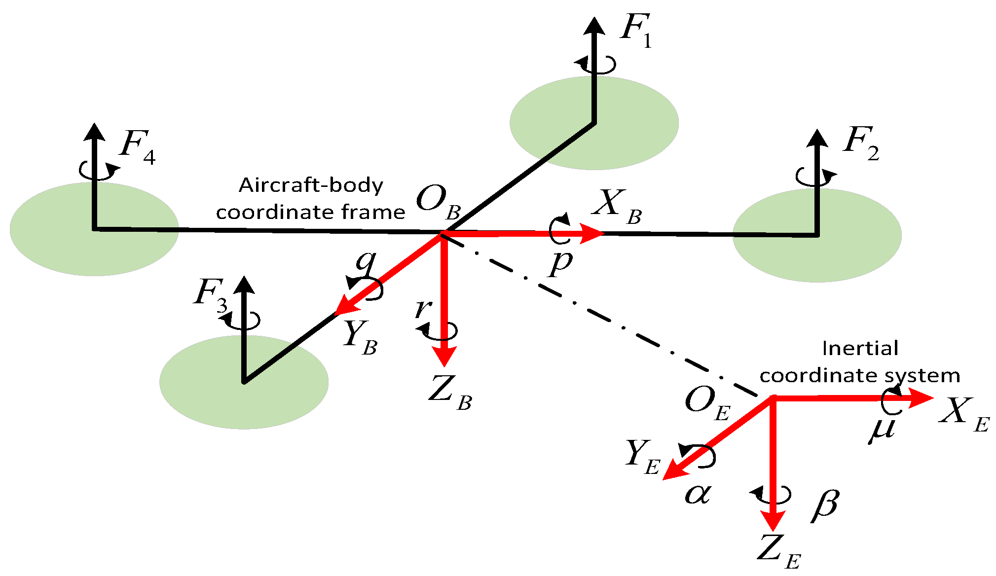
2.1. Attitude Dynamics of Quadrotor UAV

2.1.1. Attitude Angle Dynamic Equation

In order to describe the attitude states of the quadrotor UAV, the aircraft-body coordinate frame $O_B{X}_B{Y}_B{Z}_B$ and inertial coordinate frame $O_E{X}_E{Y}_E{Z}_E$ are brought into this work, as shown in Figure 1.

$$\begin{array}{c}\hfill \dot{\gamma }=\Re \left(\gamma \right)\omega \end{array}$$

(1)

where $\gamma ={[\alpha ,\beta ,\mu ]}^T$ represents the attitude angle vector of a quadrotor UAV. $\omega ={[p,q,r]}^T$ stands for the attitude angular velocity vector of a quadrotor UAV in the aircraft-body coordinate system. $\Re \left(\gamma \right)$ represents the transformation matrix from the aircraft-body coordinate system to the inertial coordinate system, and yields

$$\begin{array}{c}\hfill \Re \left(\gamma \right)=\left[\begin{array}{ccc}1& \sin \alpha \tan \beta & \cos \alpha \tan \beta \\ 0& \cos \alpha & -\sin \alpha \\ 0& \sin \alpha \sec \beta & \cos \alpha \sec \beta \end{array}\right]\end{array}$$

(2)

2.1.2. Attitude Angular Rate Dynamics

As depicted in Figure 1, the attitude angular rate dynamic of a quadrotor UAV with uncertainty of inertial matrix, system uncertainty, and external disturbance, and one has

$$\begin{array}{c}\hfill (J^{\ast }+\Delta J)\dot{\omega }=-{\omega }^{\times }(J^{\ast }+\Delta J)\omega +\Lambda +\upsilon +d\end{array}$$

(3)

where $J^{\ast }\in R^{3\times 3}$ represents the nominal inertial matrix, and the external disturbance moment is denoted by d. Furthermore, the operator ${\omega }^{\times }$ working on the vector $\omega ={[p,q,r]}^T$ results in that

$$\begin{array}{c}\hfill {\omega }^{\times }=\left[\begin{array}{ccc}0& -r& q\\ r& 0& -p\\ -q& p& 0\end{array}\right]\end{array}$$

(4)

Through a close inspection of (3), the challenges of a quadrotor UAV considered in this work distinguish the usual fault-tolerance of a quadrotor UAV, which is the uncertainty of inertial matrix ($\Delta J$) combined with its inducing system uncertainty as well as the eccentric moment. The details are analyzed as follows:

(a) Uncertainty of inertial matrix. The uncertainty $\Delta J$, as shown in (3), represents an uncertain part of $J^{\ast }$, which is derived from a movement of the mass center of a quadrotor UAV, denoted as $\overline{\rho }={[\Delta x,\Delta y,\Delta z]}^T$. By the aid of Varignon’s theorem and Parallel-Axis Theorem, it yields

$$\begin{array}{c}\hfill \Delta J=\left[\begin{array}{ccc}\Delta J_{xx}& -J_{xy}& -J_{xz}\\ -J_{xy}& \Delta J_{yy}& -J_{yz}\\ -J_{xz}& -J_{yz}& \Delta J_{zz}\end{array}\right]\end{array}$$

(5)

where $J_{xy},J_{xz}$, and $J_{yz}$ are the products of inertia, and $\Delta x,\Delta y$, and $\Delta z$ stand for the three components of the offset vector $\overline{\rho }$ along the air-craft body coordinate frame $O_B{X}_B{Y}_B{Z}_B$, as shown in Figure 1. The details are shown as follows [21]:

$$\begin{array}{cc}\hfill \Delta J_{xx}& =m(\Delta y^2+\Delta z^2),\Delta J_{yy}=m(\Delta x^2+\Delta z^2),\hfill \\ \hfill \Delta J_{zz}& =m(\Delta x^2+\Delta y^2),J_{xy}=m\Delta x\Delta y,J_{xz}=m\Delta x\Delta z,\hfill \\ \hfill J_{yz}& =m\Delta y\Delta z\hfill \end{array}$$

(6)

where m denotes the mass of a quadrotor UAV. It should be pointed that the inverse matrix of the inertial matrix with unknown $\Delta J$ suffers from the risk of being a singular matrix, which causes the failure of usual control algorithms that depend on the inverse matrix of J, for instance, adaptive control, sliding mode control, etc.

(b) System uncertainty. Based on (3), it yields that the system uncertainty caused by $\Delta J$ is hard to separate from $-{(J^{\ast }+\Delta J)}^{-1}{\omega }^{\times }(J^{\ast }+\Delta J)\omega$. In addition, because of products of inertia caused by $\Delta J$, the system uncertainties analyzed above further aggravate the coupling between the longitudinal and lateral dynamics of a quadrotor UAV, making a huge challenge for the FTC controller design.

(c) Eccentric moment induced by $\Delta J$. The eccentric moment $\Lambda$, derived from ${\Delta }_x,{\Delta }_y,{\Delta }_z$, can be modeled as

$$\Lambda =\left[\begin{array}{ccc}0& -{\upsilon }_z& {\upsilon }_y\\ {\upsilon }_z& 0& -{\upsilon }_x\\ -{\upsilon }_y& {\upsilon }_x& 0\end{array}\right]\left[\begin{array}{c}\Delta x\\ \Delta y\\ \Delta z\end{array}\right]={\Theta }^{\times }\varsigma$$

(7)

where $\upsilon ={[{\upsilon }_x,{\upsilon }_y,{\upsilon }_z]}^T$ are the control moment, which is produced by $F_1,F_2,\cdots ,F_4$, as shown in Figure 1. In terms of the control moment, $\upsilon ={[{\upsilon }_x,{\upsilon }_y,{\upsilon }_z]}^T$, ${\upsilon }_x,{\upsilon }_y$, and ${\upsilon }_z$ denote the rolling, pitching, yawing moments, respectively. The corresponding details are delivered in the following subsection.

2.2. Actuator Fault and System Input Saturation

In this work, the partial loss of efficiency fault of actuator combined with system input saturation constraints is taken into consideration. Thus, the system control input of (3) is delivered as

$$\begin{array}{c}\hfill \upsilon =Fu\left(\tau \right)+\overline{u}\end{array}$$

(8)

where $u\left(\tau \right)$ stands for the control input with saturation constraints. $F=\mathrm{diag}\{l_1,\cdots ,l_8\}$ with $0\le l_i\le 1(l_i=1,\cdots ,8)$ represents the fault matrix that reflects the health condition of the corresponding actuator, and $\overline{u}$ represents the stuck fault of a actuator. Subsequently, $u\left(\tau \right)$ can be formulated as $u\left(\tau \right)={[\mathrm{sat}\left({\tau }_1\right),\mathrm{sat}\left({\tau }_2\right),\mathrm{sat}\left({\tau }_3\right)]}^T$, which has

$$u\left({\tau }_i\right)=\mathrm{sat}\left({\tau }_i\right)=\left\{\begin{array}{c}{u}_{\tau i\max },\\ {\tau }_i,\\ u_{\tau i\min },\end{array}\begin{array}{c}{\tau }_i>u_{\tau i\max }\\ \left|{\tau }_i\right|\le u_{\tau i\max }\\ {\tau }_i<-u_{\tau i\max }\end{array}\right.$$

(9)

where $u_{\tau i\max }$ is the maximum moment produced by $F_1,F_2,\cdots ,F_4$, as shown in Figure 1. For streamlining the analysis, a smooth function is adopted to approximate (9), and we have

$$\begin{array}{c}\hfill u\left(\tau \right)=\kappa \left(\tau \right)+\epsilon \left(\tau \right)\end{array}$$

(10)

where $\kappa \left(\tau \right)={[{\kappa }_1\left({\tau }_1\right),{\kappa }_2\left({\tau }_2\right),{\kappa }_3\left({\tau }_3\right)]}^T$. With the aid of hyperbolic tangent function, ${\kappa }_i\left({\tau }_i\right)$ is obtained as

$$\begin{array}{c}\hfill {\kappa }_i\left({\tau }_i\right)=u_{\tau i\max }tanh\left({\tau }_i/\phantom{{\tau }_i{u}_{\tau i\max }}{u}_{\tau i\max }\right)\end{array}$$

(11)

where $\epsilon \left(\tau i\right)$ is the approximation error vector satisfying $\left|{\epsilon }_{\tau i}\left({\nu }_i\right)\right|=\left|sat\left({\nu }_i\right)-{\kappa }_{\tau i}\left({\nu }_i\right)\right|\le u_{\tau imax}(1-tanh\left(1\right))$. Furthermore, drawing support from mean-value theorem combined with $\kappa \left(0\right)=0$, according to [20], ${\kappa }_i\left({\tau }_i\right)$ is further modified as

$$\begin{array}{c}\hfill {\kappa }_i\left({\tau }_i\right)=\frac{\partial {\kappa }_i(·)}{\partial {\tau }_i}{\tau }_i=h_i{\nu }_i\end{array}$$

(12)

As a result, the system control input $\upsilon$ can be further modified as

$$\begin{array}{c}\hfill \upsilon ={\rm Y}\tau +F\epsilon \left(\tau \right)+\overline{u}\end{array}$$

(13)

where ${\rm Y}=diag\left(l_i{h}_i\right),i=1,2,\cdots ,3$. Based on the definition ${\rm Y}$ shown in (13), ${\rm Y}$ is a time-varying coefficient matrix reflecting the information of actuator fault and input saturation.

2.3. Problem Statement

This work is devoted to proposing an adaptive fault-tolerant control for attitude tracking of a quadrotor UAV to achieve the the following two targets, despite the presence of uncertainty of $\Delta J$ combined with its seducing system uncertainties and eccentric moment, and actuator fault and input saturation:

$Q_1$: The system output $\gamma$ tracks the desired trajectory ${\gamma }_c$, while the steady-state behavioral boundedness of the attitude angles ($\varphi ,\theta$, and $\psi$) is preserved.

$Q_2$: All signals in the closed-loop systems are bounded.

Before proceeding further, the following assumptions should be made.

Assumption A1.

The desired tracking command signals ${\gamma }_c$ is continuous and bounded.

Assumption A2.

The inverse of the inertial matrix $J=(J^{\ast }+\Delta J)$ exists.

Assumption A3.

The effects of eccentric moment Λ is bounded. In addtiton, the disturbance satisfies $∥d∥\le {\ell }_d$, where ${\ell }_d$ is the unknown constant satisfying ${\ell }_d>0$.

Remark 1.

Under Assumption 2, the inertial matrix $(J+\Delta J)$ is an invertible matrix, but the inverse of $(J+\Delta \widehat{J})$ may not exist because of the estimation of $\Delta \widehat{J}$ by estimator.

3. Preliminary Knowledge

In this section, some definitions and preliminary results, applied for the control design and the closed-loop stability analysis, are delivered as follows.

A Nussbaum gain works as a control-direction selector that can swing from positive to negative based on the control performance [22]. On account of ${\rm Y}$ (13) being a time-varying coefficient matrix, the Nussbaum gain technique is adopted in this work to handle this challenge.

Definition 1.

A function $N(·)$, named as Nussbaum-type function, possesses the following characters [20,22]:

$$\begin{array}{c}\hfill \underset{\theta \to \infty }{\lim }\inf \frac{1}{\theta }{\int }_0^{\theta }N(\Phi )\Phi =-\infty ,\underset{\theta \to \infty }{\lim }\sup \frac{1}{\theta }{\int }_0^{\theta }N(\Phi )\Phi =+\infty \end{array}$$

(14)

According to [20], the Nussbaum-type function of this work is selected as

$$\begin{array}{c}\hfill N(\Phi )=e^{{\Phi }^2/\phantom{{\Phi }^{2}2}2}({\Phi }^2+2)sin(\Phi )\end{array}$$

(15)

where Φ is the state of a Nussbaum-type function.

Lemma 1

([22]). $V\left(t\right)$ and ${\Phi }_i\left(t\right)(i=1,2,\cdots ,N)$ are smooth functions in $[0,t_f)$, satisfying $V\left(t\right)\ge 0$, ${\Phi }_i\left(0\right)=0$. If $N(·)$ is chose as (15) and the following inequality maintains

$$\begin{array}{c}\hfill V\left(t\right)\le {\hslash }_0+e^{-{\hslash }_{1}t}\sum _{i=1}^N{\int }_0^t(-{\sigma }_i\left(\lambda \right)N\left({\Phi }_i\left(\lambda \right)\right)+1){\dot{\Phi }}_i\left(\lambda \right)e^{{\hslash }_1\lambda }d\lambda \end{array}$$

(16)

where ${\hslash }_0$ is a bounded constant, and parameter ${\hslash }_1$ satisfies ${\hslash }_1>0$. ${\sigma }_i\left(t\right)\ne 0$ is a time-varying parameter which is selected from the unknown set ${\Pi }_{\sigma }:=[{\psi }^{-},{\psi }^{+}]$ (all ${\sigma }_i\left(t\right)$ have the same sign). And then, it indicates that $V\left(t\right)$, ${\Phi }_i\left(t\right)$, ${\displaystyle \sum _{i=1}^N}{\int }_0^t{\sigma }_i\left(\lambda \right)N\left({\Phi }_i\left(\lambda \right)\right){\dot{\Phi }}_i\left(\lambda \right)d\lambda$ are bounded on $[0,t_f)$.

4. Integral Reinforcement Learning-Based Adaptive Neural Network Fault-Tolerant Control

As shown in Figure 2, an adaptive FTC scheme based on integral reinforcement learning-based (IRL-based) adaptive neural network (NN) fault-tolerant control under the backstepping frame is proposed, ensuring that the system states can maintain in the designed constraints. Even if the boundary is crossed, it can be pulled back to the boundary by means of a designed penalty function with reinforcement learning.

For this purpose, in the light of backstepping derivation, the following coordinate transformation is taken into consideration: $z_{1i}=\frac{{\gamma }_i^{}}{k_{bi}^{}},i=1,2,3$, $z_2=\gamma -{\gamma }_c$ and $z_3=\omega -{\omega }_c$, where ${\omega }_c$ is a virtual control law to be designed at a later stage. The details are shown as follows:

4.1. State Constraints Penalty Function by Critic NN

For the control target that the attitude states remain in a constraint region without violation due to the demand of FTC control, it can be achieved by means of constraining $z_1$ satisfies $z_1^T{z}_1={\displaystyle \sum _{i=1}^3}\frac{{\gamma }_i^2}{k_{bi}^2}<c_{\kappa }$ all the time. Even if the boundary is crossed, it can still be pulled back. To this aim, inspired by the idea of reinforcement learning algorithm, the following discount returns are designed:

$$\begin{array}{c}\hfill \Gamma \left(t\right)={\int }_t^{\infty }{\overline{\lambda }}^{\frac{-\zeta +t}{T}}\kappa \left(z_1\left(\zeta \right)\right)d\zeta \end{array}$$

(17)

where $T>0$ denotes a small integral reinforcement interval. A discount factor in this work is denoted as $\overline{\lambda }\in (0,1)$, which can decrease the effects of a current reward for the future. When $z_1^T{z}_1={\displaystyle \sum _{i=1}^3}\frac{{\gamma }_i^2}{k_{bi}^2}<c_{\kappa }$ is satisfied, it means that the state constraint objective is achieved. The $\Gamma \left(t\right)$ will not increase, and it can be inferred that the smaller $\Gamma \left(t\right)$, the better. Conversely, the controller should be adjusted to make $z_1,z_2$, and $\Gamma \left(t\right)$ smaller even if there exists uncertainties caused by $\Delta J$, eccentric moment, actuator fault, etc. Therefore, it infers that the desired value ${\Gamma }_d$ is ${\Gamma }_d={[0,0,0]}^T$, and the immediate reward $\kappa \left(z_1\right)={[\kappa \left(z_{11}\right),\kappa \left(z_{12}\right),\kappa \left(z_{13}\right)]}^T$ can be designed as follows:

$$\kappa \left(z_{1i}\left(\zeta \right)\right)=\left\{\begin{array}{c}0\\ 1\end{array}\begin{array}{c}\\ \end{array}\begin{array}{c}\\ \end{array}\begin{array}{c}if\\ if\end{array}\begin{array}{c}{z_{1i}}^2\le c_{\kappa i}\\ {z_{1i}}^2>c_{\kappa i}\end{array}\right.,\zeta \in [t-T,t)$$

(18)

where a small threshold is represented by $c_{\kappa i}>0$. In this work, the control strategy is made that $\kappa \left(z_{1i}\right)=0$ reflects a good control performance, while $\kappa \left(z_{1i}\right)=1$ results in a bad control performance, which means that $\Gamma \left(t\right)$ will be increased. The current control should be adjusted to decrease the increase of $\Gamma \left(t\right)$ so that the out of bounds state $z_1$ can return to the constraint area again.

Afterwards, resorting to Bellman error iteration, $\Gamma (t-T)$ and $\Gamma \left(t\right)$ yield

$$\begin{array}{cc}\hfill \Gamma (t-T)& ={\int }_{t-T}^{\infty }{\varrho }^{\frac{-\zeta +t-T}{T}}\kappa \left(z_1\left(\zeta \right)\right)d\zeta ={\overline{\lambda }}^{-1}\Gamma \left(t\right)+{\int }_{t-T}^t{\overline{\lambda }}^{\frac{-\zeta +t-T}{T}}\kappa \left(z_1\left(\zeta \right)\right)d\zeta \hfill \\ \hfill & ={\overline{\lambda }}^{-1}(\Gamma \left(t\right)+{\kappa }_c)\hfill \end{array}$$

(19)

where ${\kappa }_c$ is defined as ${\kappa }_c=max\{0,{\int }_{t-T}^t{\overline{\lambda }}^{\frac{-\zeta +t}{T}}\kappa \left(z_1\left(\zeta \right)\right)d\zeta \}$ that is the value cost in the interval $[t-T,t)$, where $∥{\kappa }_c∥\le b_{{\kappa }_c}$ with a positive constant $b_{{\kappa }_c}$. In addition, to overcome the vibration caused by operator max, in this work, the approximation of ${\widehat{\kappa }}_c={[{\widehat{\kappa }}_{c1},{\widehat{\kappa }}_{c2},{\widehat{\kappa }}_{c3}]}^T$ is introduced by means of adaptive control.

On the basis of (18), ${\int }_{t-T}^t{\overline{\lambda }}^{\frac{-\zeta +t}{T}}\kappa \left(z_{1i}\left(\zeta \right)\right)d\zeta$ can be further deduced:

$${\int }_{t-T}^t{\overline{\lambda }}^{\frac{-\zeta +t}{T}}\kappa \left(z_{1i}\left(\zeta \right)\right)d\zeta =\left\{\begin{array}{c}0\\ \frac{T}{\ln \overline{\lambda }}(\overline{\lambda }-1)\end{array}\right.\begin{array}{c}if\\ if\end{array}\begin{array}{c}{z}_{1i}{\left(t\right)}^2\le c_{\kappa i}\\ z_{1i}{\left(t\right)}^2>c_{\kappa i}\end{array}$$

(20)

Since the future system information is involved in $\Gamma \left(t\right)$, as shown in (17), it is difficult to solve. According to [23,24,25], based on the value function approximation technique and Bellman Optimality Equation, a critic RBFNN is utilized in this work to handle this solving problem, and we have

$$\begin{array}{c}\hfill \Gamma \left(t\right)=W_c^{\ast }{\mathrm{H}}_c\left(x_c\left(t\right)\right)+{\mathrm{O}}_c\left(x_c\left(t\right)\right)\end{array}$$

(21)

where $W_c^{\ast T}$ stands for the ideal weight, satisfying that ${∥W_c^{\ast }∥}_F\le b_{Wc}$ and $b_{Wc}$ is a positive constant. $l_c$ is the number of hidden layers, and $x_c$ stands for the input of the RBFNN applied in this work. ${\mathrm{H}}_c\left(x_c\right)$ is the Gaussian basis function of RBFNN. It is also assumed that $∥{\mathrm{H}}_c\left(x_c\right)∥\le b_{{\mathrm{H}}_c}$, where $b_{{\mathrm{H}}_c}$ is a positive constant, so is ${\mathrm{O}}_c\left(x_c\right)$, satisfying $∥{\mathrm{O}}_c\left(x_c\right)∥\le b_{{\mathrm{O}}_c}$ with constrained boundary $b_{{\mathrm{O}}_c}>0$. Owing to the ideal weight $W_c^{\ast }$ being unknown, $\Gamma \left(t\right)$ is estimated in real time with following form:

$$\begin{array}{c}\hfill \widehat{\Gamma }\left(t\right)={\widehat{W}}_c^T{\mathrm{H}}_c\left(x_c\left(t\right)\right)\end{array}$$

(22)

In addition, the estimation of $\Gamma (t-T)$ follows:

$$\begin{array}{c}\hfill \widehat{\Gamma }(t-T)={\widehat{W}}_c^T{\mathrm{H}}_c\left(x_c(t-T)\right)\end{array}$$

(23)

Then, the temporal difference error is denoted as

$$\begin{array}{cc}\hfill e_{{\Gamma }_c}& =\widehat{\Gamma }\left(t\right)-\overline{\lambda }\widehat{\Gamma }(t-T)+{\widehat{\kappa }}_c\hfill \\ \hfill & ={\tilde{W}}_c^T\Delta {\mathrm{H}}_c\left(t\right)+{\widehat{\kappa }}_c+W_c^{\ast T}\Delta {\mathrm{H}}_c\left(t\right)\hfill \end{array}$$

(24)

where $\Delta {\mathrm{H}}_c\left(t\right)=[{\mathrm{H}}_c\left(x_c\left(t\right)\right)-\overline{\lambda }{\mathrm{H}}_c\left(x_c(t-T)\right)]$, resulting in $∥\Delta {\mathrm{H}}_c\left(t\right)∥\le (1+\overline{\lambda })b_{{\mathrm{H}}_c}$. The adaptive laws of ${\widehat{W}}_c$ and ${\widehat{\kappa }}_c$ are designed as follows: ${\widehat{W}}_c$ is updated by

$$\begin{array}{cc}\hfill {\dot{\widehat{W}}}_c& =-{\Lambda }_c\Delta {\mathrm{H}}_c\left(t\right){[{\widehat{W}}_c^T\Delta {\mathrm{H}}_c\left(t\right)+{\widehat{\kappa }}_c]}^T-{\ell }_c{\Lambda }_c{\widehat{W}}_c\hfill \\ \hfill {\dot{\widehat{\kappa }}}_c& =-{\eta }_{\kappa }{l}_{W_c}{\widehat{W}}_c^T\Delta {\mathrm{H}}_c\left(t\right)-{\eta }_{\kappa }{l}_{{\kappa }_c}{\widehat{\kappa }}_c-{\eta }_{\kappa }p{\left(z_2^T{\ell }_{\Gamma }{\widehat{W}}_c^T{\mathrm{H}}_c\left(x_c\right)\right)}^T\hfill \end{array}$$

(25)

where ${\Lambda }_c=diag\{{\Lambda }_{c1},{\Lambda }_{c2},{\Lambda }_{c3}\}>0$ denotes the learning rate matrix, combined with ${\ell }_c>0$. Besides, ${\tilde{W}}_c={\widehat{W}}_c-W_c^{\ast }$ stands for the weight error for critic NN, so does ${\tilde{\kappa }}_c$. The estimation error is defined as ${\tilde{\kappa }}_c=\mathbf{0}-{\widehat{\kappa }}_c$.

4.2. Attitude Angle Controller Design with State Constraints by Critic NN

As for the attitude tracking error $z_2$ under the constraints of system states (namely, $z_1^T{z}_1<c_{\kappa }$), a control law based on the backstepping control is designed to ensure that the state constraints $z_1$ are not violated and the tracking error $z_2$ is small enough. To this aim, the candidate Lyapunov function is delivered as

$$\begin{array}{cc}\hfill V_1& =\frac{1}{2}{z}_2^T{z}_2+\frac{{\ell }_{W_c}}{2}\mathrm{tr}\left({\tilde{W}}_c^T{\Lambda }_c^{-1}{\tilde{W}}_c\right)+\frac{1}{2{\eta }_{{\kappa }_c}}{\tilde{\kappa }}_c^T{\tilde{\kappa }}_c\hfill \\ \hfill & =V_{11}+V_{12}\hfill \end{array}$$

(26)

where ${\ell }_{W_c}$ is a positive coefficient used for theoretical analysis. Besides, $V_{11}=\frac{1}{2}{z}_2^T{z}_2$, and the remaining items make up $V_{12}$. And then, taking the time derivative of $V_{11}$ gives

$$\begin{array}{c}\hfill {\dot{V}}_{11}=z_2^T{\dot{z}}_2=z_2^T(\Re (z_3+{\omega }_c)-{\dot{\gamma }}_c)\end{array}$$

(27)

where $i=1,2,3$. Ideally, the intermediate controller ${\omega }_c$ is designed as

$$\begin{array}{cc}\hfill {\omega }_c& =\Re {\left(\gamma \right)}^{-1}(-k_1{z}_2+{\dot{\gamma }}_c-{\ell }_{\Gamma }{\widehat{W}}_c^T{\mathrm{H}}_c\left(x_c\left(t\right)\right)p^T{\widehat{\kappa }}_c)\hfill \end{array}$$

(28)

where $k_1$ is symmetric positive definite. $p={\left[\begin{array}{ccc}1& 1& 1\end{array}\right]}^T$.

As for $V_{11}$, by substituting (28) into (27), one has

$$\begin{array}{c}\hfill {\dot{V}}_{11}=-z_2^T{k}_1{z}_2+z_2^T\Re z_3-z_2^T{\ell }_{\Gamma }{\widehat{W}}_c^T{\mathrm{H}}_c\left(x_c\right)p^T{\widehat{\kappa }}_c\end{array}$$

(29)

Furthermore, the derivative of $V_{12}$ is obtained as

$$\begin{array}{cc}\hfill {\dot{V}}_{12}& =l_{W_c}\mathrm{tr}\left({\tilde{W}}_c^T{\Lambda }_c^{-1}{\dot{\tilde{W}}}_c\right)+\frac{1}{{\eta }_{\kappa }}{\tilde{\kappa }}_c^T{\dot{\tilde{\kappa }}}_c=-l_{W_c}\mathrm{tr}({\tilde{W}}_c^T\Delta {\Phi }_c\left(t\right){[{\tilde{W}}_c^T\Delta {\Phi }_c\left(t\right)+W_c^{\ast T}\Delta {\Phi }_c\left(t\right)]}^T)\hfill \\ \hfill & -l_{W_c}{\ell }_c\mathrm{tr}\left({\tilde{W}}_c^T{\tilde{W}}_c\right)-l_{W_c}{\ell }_c\mathrm{tr}\left({\tilde{W}}_c^T{W}_c^{\ast }\right)-l_{W_c}\mathrm{tr}({\tilde{W}}_c^T\Delta {\Phi }_c\left(t\right){\widehat{\kappa }}_c^T)+\frac{1}{{\eta }_{\kappa }}{\tilde{\kappa }}_c^T{\dot{\widehat{\kappa }}}_c\hfill \\ \hfill & \le -l_{W_c}\mathrm{tr}\left({\tilde{W}}_c^T(\Delta {\Phi }_c\left(t\right)\Delta {\Phi }_c{\left(t\right)}^T+{\ell }_{c}I){\tilde{W}}_c\right)+l_{W_c}{∥{\tilde{W}}_c∥}_F(∥\Delta {\Phi }_c\left(t\right)∥∥W_c^{\ast T}\Delta {\Phi }_c\left(t\right)∥+{\ell }_c{∥{\tilde{W}}_c^{\ast }∥}_F)\hfill \\ \hfill & -l_{W_c}\mathrm{tr}({\tilde{W}}_c^T\Delta {\Phi }_c\left(t\right){\widehat{\kappa }}_c^T)+\frac{1}{{\eta }_{\kappa }}{\tilde{\kappa }}_c^T{\dot{\widehat{\kappa }}}_c\hfill \\ \hfill & \le -l_V{k}_c\mathrm{tr}\left({\tilde{W}}_c^T{\tilde{W}}_c\right)+b_{V_c}{∥{\tilde{W}}_c∥}_F-l_{W_c}\mathrm{tr}({\tilde{W}}_c^T\Delta {\Phi }_c\left(t\right){\widehat{\kappa }}_c^T)-\frac{1}{{\eta }_{\kappa }}{\tilde{\kappa }}_c^T{\dot{\widehat{\kappa }}}_c\hfill \end{array}$$

(30)

where $b_{V_c}=l_{W_c}{(1+\lambda )}^2{b}_{H_c}^2{b}_{W_c}+l_{W_c}{\ell }_c{b}_{W_c}$.

Further, ${\dot{V}}_1$ is obtained as

$$\begin{array}{cc}\hfill {\dot{V}}_1& ={\dot{V}}_{11}+{\dot{V}}_{12}\hfill \\ \hfill & \le -z_2^T{k}_1{z}_2+z_2^T\Re z_3-l_{W_c}{k}_c\mathrm{tr}\left({\tilde{W}}_c^T{\tilde{W}}_c\right)+b_{V_c}{∥{\tilde{W}}_c∥}_F+l_{W_c}\mathrm{tr}(W_c^{\ast T}\Delta {\Phi }_c\left(t\right){\tilde{\kappa }}_c^T)+l_{{\kappa }_c}{{\tilde{\kappa }}_c}^T{\widehat{\kappa }}_c\hfill \\ \hfill & \le -z_2^T{k}_1{z}_2+z_2^T\Re z_3-l_{W_c}{k}_c\mathrm{tr}\left({\tilde{W}}_c^T{\tilde{W}}_c\right)+b_{V_c}{∥{\tilde{W}}_c∥}_F-\frac{l_{{\kappa }_c}}{2}{∥{\tilde{\kappa }}_c∥}_F^2+\frac{l_{{\kappa }_c}}{2}{∥{\kappa }_c∥}_F^2\hfill \\ \hfill & +l_{W_c}{b}_{W_c}{b}_{H_c}(1+\overline{\lambda }){∥{\tilde{\kappa }}_c^{}∥}_F\hfill \end{array}$$

(31)

where

$$\begin{array}{cc}\hfill & l_{{\kappa }_c}{{\tilde{\kappa }}_c}^T{\widehat{\kappa }}_c\le -\frac{l_{{\kappa }_c}}{2}{∥{\tilde{\kappa }}_c∥}_F^2+\frac{l_{{\kappa }_c}}{2}{∥{\kappa }_c∥}_F^2\hfill \\ \hfill & l_{W_c}\mathrm{tr}(W_c^{\ast T}\Delta {\Phi }_c\left(t\right){\tilde{\kappa }}_c^T)\le l_{W_c}{b}_{W_c}{b}_{H_c}(1+\overline{\lambda }){∥{\tilde{\kappa }}_c^{}∥}_F\hfill \\ \hfill & -\frac{l_{{\kappa }_c}}{4}{∥{\tilde{\kappa }}_c∥}_F^2+l_{W_c}{b}_{W_c}{b}_{H_c}(1+\overline{\lambda }){∥{\tilde{\kappa }}_c^{}∥}_F\le l_{W_c}^2{b}_{W_c}^2{b}_{H_c}^2{(1+\overline{\lambda })}^2/\phantom{l_{W_c}^2{b}_{W_c}^2{b}_{H_c}^2{(1+\overline{\lambda })}^2{l}_{{\kappa }_c}}{l}_{{\kappa }_c}\hfill \end{array}$$

(32)

In what follows, ${\dot{V}}_1$ is further deduced as

$$\begin{array}{cc}\hfill {\dot{V}}_1& \le -z_2^T{k}_1{z}_2+z_2^T\Re z_3-l_{W_c}{k}_c\mathrm{tr}\left({\tilde{W}}_c^T{\tilde{W}}_c\right)+b_{V_c}{∥{\tilde{W}}_c∥}_F\hfill \\ \hfill & -\frac{l_{{\kappa }_c}}{4}{∥{\tilde{\kappa }}_c∥}_F^2+l_{W_c}^2{b}_{W_c}^2{b}_{H_c}^2{(1+\overline{\lambda })}^2/\phantom{l_{W_c}^2{b}_{W_c}^2{b}_{H_c}^2{(1+\overline{\lambda })}^2{l}_{{\kappa }_c}}{l}_{{\kappa }_c}+\frac{l_{{\kappa }_c}}{2}{∥{\kappa }_c∥}_F^2\hfill \\ \hfill & \le -{\lambda }_{min}\left(k_1\right){∥z_2∥}^2+z_2^T\Re z_3-(l_{W_c}{k}_c-l_c)\mathrm{tr}\left({\tilde{W}}_c^T{\tilde{W}}_c\right)\hfill \\ \hfill & -\frac{l_{{\kappa }_c}}{4}{∥{\tilde{\kappa }}_c∥}_F^2+b_{V_1}\hfill \end{array}$$

(33)

where

$$\begin{array}{cc}\hfill & -l_c{∥{\tilde{W}}_c∥}_F^2+b_{V_c}{∥{\tilde{W}}_c∥}_F\le b_{V_c}^2/\phantom{\left[b_{V_c}^2\right]2l_c}2l_c\hfill \\ \hfill & b_{V_1}=b_{V_c}^2/\phantom{b_{V_1}=b_{V_c}^{2}2l_c}2l_c+l_{W_c}^2{b}_{W_c}^2{b}_{H_c}^2{(1+\overline{\lambda })}^2/\phantom{l_{W_c}^2{b}_{W_c}^2{b}_{H_c}^2{(1+\overline{\lambda })}^2{l}_{{\kappa }_c}}{l}_{{\kappa }_c}+\frac{l_{{\kappa }_c}}{2}{∥{\kappa }_c∥}_F^2\hfill \end{array}$$

4.3. Attitude Angular Rate Controller Design Resorting to Action NN

In this part, the final control law is designed for $\tau$ to drive $z_3\to 0$, where the tracking error $z_3$ is defined by

$$\begin{array}{c}\hfill z_3=\omega -{\omega }_c\end{array}$$

(34)

where ${\omega }_c$ and ${\dot{\omega }}_c$ are available for controller.

By taking (34) and (13) into consideration, we have

$$\begin{array}{c}\hfill J{\dot{z}}_3=-{\omega }^{\times }J\omega +\Lambda +{\rm Y}\tau +D-J{\dot{\omega }}_c\end{array}$$

(35)

where the complex disturbance is defined as $D=F\epsilon \left(\tau \right)+\overline{u}+d$.

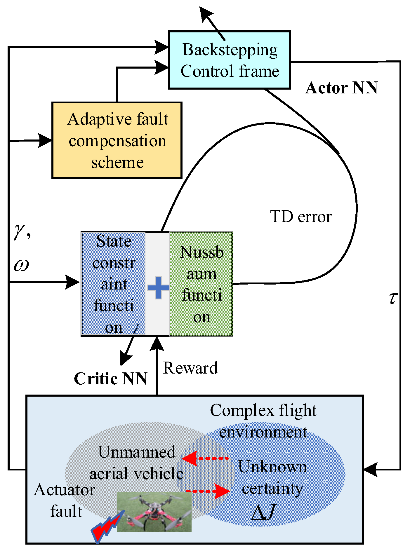
• Uncertainties of of system: Then, in order to facilitate the subsequent derivation, we define that $R=-{\omega }^{\times }J\omega -J{\dot{\omega }}_c$, drawing support from the operation rule $\Delta Jx=L\left(x\right)\theta$ [20], where $\theta ={[J_{11},J_{12},J_{13},J_{22},J_{23},J_{33}]}^T$. In this work, R can be made by can $R=\Im (·)\theta$, where $\Im (·)\in R^{3\times 6}$ is delivered as follows:

  $$\begin{array}{c}\hfill \Im (·)=-{\omega }^{\times }L\left(\omega \right)-L\left({\dot{\omega }}_c\right)\end{array}$$

  (36)
  Furthermore, by the aid of synthesized adaptive control technology, the following expression is made to reduce the calculated load problem caused by too many estimated variables ($\theta$). The details are shown as follows:

  $$\begin{array}{c}\hfill ∥\Im (·)\theta ∥\le \Psi \hslash \end{array}$$

  (37)

  where $\Psi ={∥\Im (·)∥}_F,\hslash =∥\theta ∥$. The estimation of $\tilde{\hslash }$ is defined as $\tilde{\hslash }=\hslash -\widehat{\hslash }$.
• Eccentric moment and Disturbance: For unknown disturbance and eccentric moment, an action RBFNN is established to approximate it and we have

  $$\begin{array}{c}\hfill f=\Lambda +D=W_a^{\ast }{\Phi }_a\left(x_a\left(t\right)\right)+{\mathrm{O}}_a\left(x_a\left(t\right)\right)\end{array}$$

  (38)

  where $W_a^{\ast }$ stands for the ideal weight. $x_a$ represents the input vector for actor NN. ${\varphi }_a\left(x_a\right)$ denotes the Gaussian basis function. As for ${\epsilon }_a\left(x_a\right)$, it is assumed that $∥{\epsilon }_a\left(x_a\right)∥<b_{{\epsilon }_a}$, where $b_{{\epsilon }_a}$ is a positive constant. And then, we have the real time estimation as

  $$\begin{array}{c}\hfill \widehat{f}={\widehat{W}}_a^T{\varphi }_a\left(x_a\right)\end{array}$$

  (39)
  Define the weight error for action NN:

  $$\begin{array}{c}\hfill {\tilde{W}}_a={\widehat{W}}_a-W_a^{\ast }\end{array}$$

  (40)
• Uncertainties of inertial matrix: In order to conquer the challenge caused by time-varying coefficient matrix ${\rm Y}$, as shown in (13), which is caused by actuator fault, input saturation combined with $\Delta J$, recalling Nussbaum-type function, the final control law and adaptive law are proposed as follows:

  $$\begin{array}{cc}\hfill \tau & =N_a\left(\chi \right){\varpi }_a\hfill \\ \hfill {\varpi }_a& =-k_a{z}_3-\Psi \widehat{\hslash }Tanh\left(\frac{z_3}{\vartheta }\right)-\Re z_2-{\widehat{W}}_a^T{\varphi }_a\left(x_a\right)\hfill \\ \hfill \dot{\chi }& =-k_N\mathrm{diag}\left(z_3\right){\varpi }_a\hfill \\ \hfill \dot{\widehat{\hslash }}& =\eta \Psi z_3^T\mathrm{Tanh}\left(z_3/\phantom{z_2\vartheta }\vartheta \right)-\eta l_{\hslash }\widehat{\hslash }\hfill \end{array}$$

  (41)

  where $\vartheta =k_{\vartheta }/\phantom{k_{\vartheta }(1+}(1+{∥\Im (·)∥}_{\infty })$ with $\vartheta$ and $k_{\vartheta }$ being design parameters.
• Action NN design: There are two objectives for action NN design under the uncertainties caused by $\Delta J$ and actuator fault. One is to make $z_3$ follow ${\omega }_c$ well. The other one is to make $\Gamma \left(t\right)$ minimized to its desired value ${\Gamma }_d=0$. As a consequence, the following action error is defined as

  $$\begin{array}{c}\hfill e_a=z_3+\widehat{\Gamma }\left(t\right)-{\Gamma }_d\end{array}$$

  (42)
  And then, the corresponding update law of ${\widehat{W}}_a$ is designed as

  $$\begin{array}{cc}\hfill \dot{\widehat{W_a}}& ={\Lambda }_a{\Phi }_a\left(x_a\right){[z_3+{\widehat{W}}_c^T{\Phi }_c\left(x_c\right)]}^T-k_a{\Lambda }_a{\widehat{W}}_a\hfill \end{array}$$

  (43)

  where ${\Lambda }_a=\mathrm{diag}({\Lambda }_{a1},{\Lambda }_{a2},{\Lambda }_{a3})$ is a learning rate matrix to be designed, which is a positive definite matrix.

5. Stability Analysis

In this section, the main result of this work is summarized as the following theorem.

Theorem 1.

Take a quadrotor UAV attitude tracking system depicted by (1)–(4), suffers from the uncertainty caused by $\Delta J$ and its corresponding system uncertainties and eccentric moment, with actuator faults and input saturation in consideration. When the Assumptions 1–3 hold, an adaptive fault-tolerant control strategy for attitude tracking to a quadrotor UAV is proposed in this work, consisted of (25) and (41). The following two targets are achieved, despite the presence of uncertainty of $\Delta J$ combined with its inducing system uncertainties and eccentric moment, and actuator fault and input saturation:

$Q_1$: The system output γ tracks the desired trajectory ${\gamma }_c$, while the steady-state behavioral boundedness of the attitude angles ($\varphi ,\theta$, and ψ) is preserved.

$Q_2$: All signals in the closed-loop systems are bounded.

Proof. 

The following Lyapunov function candidate is selected as:

$$\begin{array}{cc}\hfill V_2& =V_1+\frac{1}{2}{z}_3^{T}J{z}_3+\frac{1}{2\eta }{\tilde{\hslash }}^T\tilde{\hslash }+\frac{1}{2}\mathrm{tr}\left({\tilde{W}}_a^T{\Lambda }_a^{-1}{\tilde{W}}_a\right)\hfill \end{array}$$

(44)

□

Furthermore, for the first item of (44) with the properties $\mathrm{tr}\left(A^{T}A\right)={∥A∥}_F^2$, ${∥a{b}^T∥}_F\le ∥a∥∥b∥$ and $∥Aa∥\le {∥A∥}_F∥a∥$, one has:

$$\begin{array}{cc}\hfill {\dot{V}}_2& ={\dot{V}}_1+z_3^{T}J{\dot{z}}_3-\frac{1}{\eta }{\tilde{\hslash }}^T\dot{\widehat{\hslash }}+\mathrm{tr}\left({\tilde{W}}_a^T{\Lambda }_a^{-1}{\dot{\widehat{W}}}_a\right)\hfill \\ \hfill & \le (z_3^{T}P\Psi \hslash -\frac{1}{\eta }{\tilde{\hslash }}^T\dot{\widehat{\hslash }})+z_3^T(W_a^{\ast }{\varphi }_a+O_a)+\mathrm{tr}\left({\tilde{W}}_a^T{\Lambda }_a^{-1}{\dot{\widehat{W}}}_a\right)\hfill \\ \hfill & +z_3^T{\rm Y}\tau -{\lambda }_{min}\left(k_1\right){∥z_2∥}^2+z_2^T\Re z_3-\left(l_{W_c}{k}_c\right)\hfill \\ \hfill & -l_c\left)\mathrm{tr}\right({\tilde{W}}_c^T{\tilde{W}}_c-\frac{l_{{\kappa }_c}}{4}{∥{\tilde{\kappa }}_c∥}_F^2+b_{V_1}\hfill \end{array}$$

(45)

After substituting the control law and its adaptive laws (41) into (45), it follows:

$$\begin{array}{cc}\hfill {\dot{V}}_2& ={\dot{V}}_1+z_3^{T}J{\dot{z}}_3-\frac{1}{\eta }{\tilde{\hslash }}^T\dot{\widehat{\hslash }}+\mathrm{tr}\left({\tilde{W}}_a^T{\Lambda }_a^{-1}{\dot{\widehat{W}}}_a\right)\hfill \\ \hfill & \le -{\lambda }_{min}\left(k_1\right){∥z_2∥}^2-{\lambda }_{min}\left(k_a\right){∥z_3∥}^2-(l_{W_c}{k}_c-l_c)\mathrm{tr}\left({\tilde{W}}_c^T{\tilde{W}}_c\right)\hfill \\ \hfill & -\frac{l_{{\kappa }_c}}{4}{∥{\tilde{\kappa }}_c∥}_F^2+\sum _{i=1}^3\frac{1}{k_{Ni}}(-{{\rm Y}}_{i}N\left({\chi }_i\right)+1){\dot{\chi }}_i\hfill \\ \hfill & +(z_3^{T}P\Psi \hslash -\frac{1}{\eta }{\tilde{\hslash }}^T\dot{\widehat{\hslash }})-z_3^T\Psi \widehat{\hslash }tanh\left(\frac{z_3}{\vartheta }\right)\hfill \\ \hfill & +z_3^T(W_a^{\ast }{\varphi }_a+O_a)+\mathrm{tr}\left({\tilde{W}}_a^T{\Lambda }_a^{-1}{\dot{\widehat{W}}}_a\right)\hfill \\ \hfill & -z_3^T{\widehat{W}}_a^T{\varphi }_a\left(x_a\right)+b_{V_1}\hfill \end{array}$$

(46)

And then, it is further deduced that

$$\begin{array}{cc}\hfill {\dot{V}}_2& \le -{\lambda }_{min}\left(k_1\right){∥z_2∥}^2-{\lambda }_{min}\left(k_a\right){∥z_3∥}^2-(l_{W_c}{k}_c-l_c)\mathrm{tr}\left({\tilde{W}}_c^T{\tilde{W}}_c\right)\hfill \\ \hfill & -\frac{l_{{\kappa }_c}}{4}{∥{\tilde{\kappa }}_c∥}_F^2+\sum _{i=1}^3\frac{1}{k_{Ni}}(-{{\rm Y}}_{i}N\left({\chi }_i\right)+1){\dot{\chi }}_i+b_{V_1}\hfill \\ \hfill & +{\hslash }^T\Psi \sum _{i=1}^3(\left|z_{3i}\right|(1-tanh\left(\frac{\left|z_{3i}\right|}{\vartheta }\right)))-\frac{l_{\hslash }}{2}{∥\tilde{\hslash }∥}_F^2+\frac{l_{\hslash }}{2}{∥\hslash ∥}_F^2\hfill \\ \hfill & +b_{O_a}∥z_3∥+\frac{k_a{b}_{W_a}^2}{2}-\frac{k_a}{2}\mathrm{tr}\left({\tilde{W}}_a^T{\tilde{W}}_a\right)\hfill \\ \hfill & +b_{{\Phi }_a}{b}_{{\Phi }_c}{∥{\tilde{W}}_a^{}∥}_F({∥{\tilde{W}}_c^{}∥}_F+b_{W_c})\hfill \end{array}$$

(47)

Furthermore, it is obtained that

$$\begin{array}{cc}\hfill {\dot{V}}_2& \le -{\lambda }_{min}\left(k_1\right){∥z_2∥}^2-{\lambda }_{\min }\left(k_{a2}\right){∥z_3∥}^2-\frac{l_{{\kappa }_c}}{4}{∥{\tilde{\kappa }}_c∥}_F^2\hfill \\ \hfill & -(l_{W_c}{k}_c-\frac{b_{{\Phi }_a}{b}_{{\Phi }_c}}{2}-l_c)\mathrm{tr}\left({\tilde{W}}_c^T{\tilde{W}}_c\right)-\frac{l_{\hslash }}{2}{∥\tilde{\hslash }∥}_F^2\hfill \\ \hfill & -(\frac{k_a}{2}-\frac{b_{{\Phi }_a}{b}_{{\Phi }_c}}{2}-l_a)\mathrm{tr}\left({\tilde{W}}_a^T{\tilde{W}}_a\right)\hfill \\ \hfill & +\sum _{i=1}^3\frac{1}{k_{Ni}}(-{{\rm Y}}_{i}N\left({\chi }_i\right)+1){\dot{\chi }}_i+b_{V_1}+b_{V_2}\hfill \end{array}$$

(48)

where $b_{V_2}=\frac{b_{O_a}^2}{4{\lambda }_{min}\left(k_{a1}\right)}+\frac{k_a{b}_{W_a}^2}{2}+\frac{b_{{\Phi }_a}^2{b}_{{\Phi }_c}^2{b}_{W_c}^2}{4l_a}+\frac{l_{\hslash }}{2}{∥\hslash ∥}_F^2+3\alpha k_{\vartheta }∥\theta ∥$. The following inequalities are used:

$$\begin{array}{cc}\hfill -l_a{∥{\tilde{W}}_a∥}_F^2& +b_{{\Phi }_a}{b}_{{\Phi }_c}{b}_{W_c}{∥{\tilde{W}}_a∥}_F\le \frac{{\left(b_{{\Phi }_a}{b}_{{\Phi }_c}{b}_{W_c}\right)}^2}{4l_a}\hfill \\ \hfill -{\lambda }_{min}\left(k_{a1}\right){∥z_3∥}^2& +b_{O_a}∥z_3∥\le \frac{b_{O_a}^2}{4{\lambda }_{min}\left(k_{a1}\right)}\hfill \\ \hfill l_{\hslash }{\tilde{\hslash }}^T\widehat{\hslash }& \le -\frac{l_{\hslash }}{2}{∥\tilde{\hslash }∥}_F^2+\frac{l_{\hslash }}{2}{∥\hslash ∥}_F^2\hfill \end{array}$$

(49)

Finally, we have

$$\begin{array}{c}\hfill {\dot{V}}_2\le -c{V}_2+b_V+\sum _{i=1}^3\frac{1}{k_{Ni}}(-{{\rm Y}}_{i}N\left({\chi }_i\right)+1){\dot{\chi }}_i\end{array}$$

(50)

where

$$\begin{array}{cc}\hfill & \begin{array}{c}c=min\{2{\lambda }_{min}\left(k_1\right),{\lambda }_{min}\left(k_{a2}\right),\frac{2l_{W_c}{k}_c-b_{{\Phi }_a}{b}_{{\Phi }_c}-2l_c}{{\lambda }_{min}\left({\Lambda }_c^{-1}\right)},\hfill \\ \frac{k_a-b_{{\Phi }_a}{b}_{{\Phi }_c}-2l_a)}{{\lambda }_{min}\left({\Lambda }_a^{-1}\right)}\}\hfill \end{array}\hfill \\ \hfill & b_V=b_{V_1}+b_{V_2}\hfill \end{array}$$

Let us define $\nu =b_V/c$. Then, multiplying both sides of (50) by $e^{ct}$, and integrating the resulting inequality over $[0,t]$, we have (in the set Z1)

$$\begin{array}{cc}\hfill V_2\left(t\right)& \le \nu +V_2\left(t\right)e^{-ct}+e^{-ct}\hfill \\ \hfill & \times \sum _{i=1}^3\frac{1}{k_{Ni}}{\int }_0^t(-{{\rm Y}}_{i}N\left({\chi }_i\left(\lambda \right)\right)+1){\dot{\chi }}_i\left(\lambda \right)e^{ct}d\lambda \hfill \end{array}$$

(51)

Since ${{\rm Y}}_i,i=1,2,3$ are constrained to the closed interval $[{\psi }^{-},{\psi }^{+}]$, then from (51) and Lemma 1, it is obtained that ${\chi }_i\left(t\right),i=1,2,3,{\displaystyle \sum _{i=1}^3}{\int }_0^t(-{{\rm Y}}_{i}N\left({\chi }_i\right)+1){\dot{\chi }}_{i}d\lambda ,V_2\left(t\right)$ are bounded on $[0,t_f)$. Then, from the positive definition of $V_2\left(t\right)$, it can be shown that $\Gamma ,z_2,z_3,{\tilde{\kappa }}_c,\tilde{\hslash },{\tilde{W}}_c,{\tilde{W}}_a$ are also bounded on $[0,t_f)$. Based on the above arguments, all closed-loop signals are bounded.

For convenience of analysis, we denote $c_B$ as the upper bound of

$$\frac{1}{k_{Ni}}\sum _{i=1}^3{\int }_0^t\left|(-{{\rm Y}}_{i}N\left({\chi }_i\right)+1){\dot{\chi }}_i\right|d\lambda ,$$

then, after straightforward algebraic manipulations, (51) reduces to

$$\begin{array}{c}\hfill V_2\left(t\right)\le \nu +c_B+V_2\left(0\right)e^{-ct}\end{array}$$

(52)

where when $t=0$, we have

$$\begin{array}{cc}\hfill V_2\left(0\right)& =\frac{1}{2}{z}_2^T\left(0\right)z_2\left(0\right)+\frac{{\ell }_{W_c}}{2}\mathrm{tr}\left({\tilde{W}}_c^T\left(0\right){\Lambda }_c^{-1}{\tilde{W}}_c\left(0\right)\right)+\frac{1}{2{\eta }_{{\kappa }_c}}{\tilde{\kappa }}_c^T\left(0\right){\tilde{\kappa }}_c\left(0\right)+\frac{1}{2}{z}_3^T\left(0\right)J{z}_3\left(0\right)\hfill \\ \hfill & +\frac{1}{2\eta }{\tilde{\hslash }}^T\left(0\right)\tilde{\hslash }\left(0\right)+\frac{1}{2}\mathrm{tr}\left({\tilde{W}}_a^T\left(0\right){\Lambda }_a^{-1}{\tilde{W}}_a\left(0\right)\right)\hfill \end{array}$$

By invoking the boundedness of $\frac{{\ell }_{W_c}}{2}\mathrm{tr}\left({\tilde{W}}_c^T{\Lambda }_c^{-1}{\tilde{W}}_c\right)$ and the relationship of $\Gamma \left(t\right)$ (17) and $\widehat{\Gamma }\left(t\right)$ (22), one may notice that $z_1\left(t\right)$ remains in the designed constrained area $z_1^T{z}_1={\displaystyle \sum _{i=1}^3}\frac{{\gamma }_i^2}{k_{bi}^2}<c_{\kappa }$ for all time. Then, with respect to the tracking error, it can be easily verified that $\frac{1}{2}{z}_2^T{z}_2\le V_2\left(t\right)\le \overline{V}$, where $\overline{V}=\nu +c_B+V_2\left(0\right)$, which would lead to [20,23]:

$$\begin{array}{c}\hfill ∥z_2∥\le \sqrt{2\overline{V}}\end{array}$$

(53)

under the $min\Gamma \left(t\right)$. Furthermore, based on ${\lambda }_{min}\left(J\right){∥z_3∥}^2\le z_3^{T}J{z}_3\le 2\overline{V}$, we have that $∥z_3∥\le \sqrt{\frac{2\overline{V}}{{\lambda }_{min}\left(J\right)}}$.

In what follows, with the properties $\mathrm{tr}\left(A^{T}A\right)={∥A∥}_F^2$, ${∥a{b}^T∥}_F\le ∥a∥∥b∥$ and $∥Aa∥\le {∥A∥}_F∥a∥$, taking the $∥{\tilde{W}}_c∥\le \sqrt{\frac{2\overline{V}}{{\ell }_{W_c}{\lambda }_{min}\left({\Lambda }_c^{-1}\right)}}$, for example, it is deduced by the following process:

$$\begin{array}{c}\hfill \frac{{\ell }_{W_c}}{2}\mathrm{tr}\left({\tilde{W}}_c^T{\Lambda }_c^{-1}{\tilde{W}}_c\right)\le \frac{{\ell }_{W_c}}{2}∥{\tilde{W}}_c^T{\Lambda }_c^{-1}{\tilde{W}}_c∥\le \frac{{\ell }_{W_c}}{2}{\lambda }_{max}\left({\Lambda }_c^{-1}\right){∥{\tilde{W}}_c∥}^2\le \overline{V}\end{array}$$

(54)

Similarly, we have that

$$\begin{array}{cc}\hfill & ∥{\tilde{W}}_a∥\le \sqrt{\frac{2\overline{V}}{{\lambda }_{min}\left({\Lambda }_a^{-1}\right)}},∥\tilde{\hslash }∥\le \sqrt{2\eta \overline{V}},∥{\tilde{\kappa }}_c∥\le \sqrt{2{\eta }_{{\kappa }_c}\overline{V}}\hfill \end{array}$$

(55)

This completes the proof of Theorem 1, and the achievement of R1 and R2 are realized.

6. Simulation Studies

Considering that a quadrotor UAV with the speed of $3\mathrm{m}/\mathrm{s}$ and an altitude of $10\mathrm{m}$, the initial attitude vector is $\gamma =[0.017,0.026,0.017]\mathrm{rad}$, and the angular rate is $\omega ={[0,0,0]}^T\mathrm{rad}/\mathrm{s}$. The reference signals are set that ${\alpha }_{\mathrm{c}}=0.087\mathrm{rad}$ during 1–8 s, ${\alpha }_{\mathrm{c}}=0.02\mathrm{rad}$ during 8–20 s and ${\alpha }_{\mathrm{c}}=0.05\mathrm{rad}$ during $t>20$ s, besides, $\beta$ is always $0\mathrm{rad}$ and $\mu$ is keeping $0.035\mathrm{rad}$. In addition, the loss of efficiency fault of actuator is set to $\lambda =diag\left\{0.2,0.17,0.2\right\}$ as the 5th second. The external disturbances of a quadrotor UAV is described as follows: ${\mathrm{d}}_{f1}=2.5sin\left(3t+0.2\right)N·m,{\mathrm{d}}_{f2}=5.5sin\left(4t\right.\left.-0.2\right)N·m$, ${\mathrm{d}}_{f3}=5.5sin\left(4t+0.2\right)N·m$. The design parameters of controller of a quadrotor UAV are that $k_1=1.23\ast I_3$, ${\ell }_{\Gamma }=0.15$. $c_{\kappa }=0.23$. $\lambda =0.97$. $k_a=1.23$, $k_N=0.8$, $\eta =0.5$. ${\Lambda }_c={\eta }_{\kappa }=0.75$, ${\Lambda }_a=0.82$. In addition, the initial center of the RBFNN is

$$\begin{array}{c}\hfill c=\left[\begin{array}{ccccccc}-1.5& -1& -0.5& 0& 0.5& 1& 1.5\\ -1.5& -1& -0.5& 0& 0.5& 1& 1.5\\ -1.5& -1& -0.5& 0& 0.5& 1& 1.5\end{array}\right]\end{array}$$

and the initial width is selected as $b=10{[1,1,1,1,1,1,1]}^T$.

In order to study the influence of uncertainty of inertial matrix caused by $\Delta J$ on the motion of a quadrotor UAV and validate the effectiveness of designed fault-tolerant controller, the simulation is carried out in two cases. In case 1, for analyzing the effects of uncertainty of inertial matrix on the attitude tracking performacne of quadrotor UAV, simulation conditions are set that the offsets of mass of center have different values along the x-axis. In case 2, under the similar simulation conditions, compared with the tracking effects of FTC strategy consisted of sliding mode control combined with nonlinear disturbance observer, the simulation results demonstrate the effectiveness of the designed state constraints strategy.

Case 1: Under the same fault-tolerant control conditions, the offset of mass of center just alone the x-axis is set that $\overline{\rho }={[\Delta x,\Delta y,\Delta z]}^T={[-4,0,0]}^{T}cm$ in the 10th second, and the corresponding simulation curves are represented by ${\left(·\right)}_3$. Similarly, ${\left(·\right)}_4$ denotes the conditions that ${[\Delta x,\Delta y,\Delta z]}^T={[-1,0,0]}^{T}cm$. ${\left(·\right)}_5$ and ${\left(·\right)}_6$ stand for the conditions that ${[\Delta x,\Delta y,\Delta z]}^T={[3,0,0]}^{T}cm$ and ${[\Delta x,\Delta y,\Delta z]}^T={[4.5,0,0]}^{T}cm$, respectively. The simulation results are shown as follows.

Based on the analysis with respect to the influence of uncertainty of inertial matrix caused by $\Delta J$ on the motion of quadrotor UAV, it covers three aspects: system uncertainties, eccentric moment, and variation of inertial matrix $J^{\ast }+\Delta J$. For the variation of $J^{\ast }$, by taking the tracking curves of attitude angles depicted in Figure 3, Figure 4 and Figure 5 for example, tracking curves of ${\alpha }_{com}$, ${\beta }_{com}$, and ${\mu }_{com}$ show a trend of divergence after the 10th second, which displays that the controller based on sliding mode control technology that rests on the inverse matrix of inertia matrix ${\left(J^{\ast }\right)}^{-1}$ can not handle the variation of inertial matrix J due to $\Delta J$. The FTC strategy of this work without the exact knowledge of ${(J^{\ast }+\Delta J)}^{-1}$ displays good tracking effects, as shown in ${(·)}_3$ of Figure 3, Figure 4, Figure 5, Figure 6, Figure 7 and Figure 8. As a result, the simulation results reveal that the FTC strategy of this work is effective. Furthermore, in order to investigate the $\Delta J$ on the attitude tracking of quadrotor UAV, some other simulations are made, as shown in the attitude tracking curves of ${(·)}_4$, ${(·)}_5$, and ${(·)}_6$ in Figure 3, Figure 4, Figure 5, Figure 6, Figure 7 and Figure 8.

With the center of mass moving away from the original centroid along the positive direction of x-axis, the tracking effects of ${\alpha }_i,{\beta }_i,{\mu }_i,i=3,\cdots ,6$ of Figure 3, Figure 4 and Figure 5 are gradually declining. When the center of mass is further from the aerodynamic center (from ${(·)}_3$ to ${(·)}_6$), the larger oscillation of the tracking curves occur, as shown in tracking curves of ${(·)}_{\alpha }$ and other response curves of Figure 3, Figure 4, Figure 5, Figure 6, Figure 7 and Figure 8. Furthermore, it would be inferred that the further center of mass leaving from the aerodynamic center leads to the larger extra control moment due to the longer arm of force. The greater offset of center of mass can result in the greater $\Delta J$ inducing system uncertainties and eccentric moment, etc., leading to huge challenges for the designed FTC controller.

Case 2: The state constrained fault-tolerant control method of quadrotor UAV based on reinforcement learning is simulated, and the rigid body attitude tracking control effect of quadrotor UAV affected by the unknown $\Delta J$ and the safety state constraint can be obtained, as shown in Figure 9 and Figure 10. Figure 9 and Figure 10 show the desired attitude and attitude angle tracking curve of a quadrotor UAV from top to bottom, as well as the comparison group (without state safety constraints). The three figures in Figure 9 and Figure 10 are the attack angle tracking curve, pitch angle tracking curve, and roll angle tracking curve of the aircraft from top to bottom. From the corresponding reference attitude command and the actual tracking effect, it can be seen that even when there is an unknown $\Delta J$ caused by $\overline{\rho }$, the control algorithm designed in this paper can still maintain a good attitude tracking and maintenance effect. However, from the perspective of the control group, when an unknown $\Delta J$ caused by $\overline{\rho }$ occurs, an abnormal eccentric moment is generated. When the system state is unconstrained, the influence of the eccentric moment will be superimposed, until 22 s, the fault-tolerant control of the system will fail, as shown in Figure 9 and Figure 10. Under the state constrained fault-tolerant control method of quadrotor UAV based on reinforcement learning, even if the boundary is crossed, it can be pulled back to the boundary by means of a designed penalty function.

7. Conclusions

In this paper, a fault-tolerant controller considering unknown inertial matrix, actuator fault, and input saturation is proposed. Contrary to the usual log-type BLF literature, a novel state-constraint mechanism is proposed, which can ensure that the system states maintain in the designed constraints. Even if the boundary is crossed, it can be pulled back to the boundary by means of a designed penalty function with reinforcement learning. Meanwhile, in order to inhibit the algorithm oscillation caused by maximum operation of ${\widehat{\kappa }}_c$, the immediate reward ${\widehat{\kappa }}_c$ is obtained with adaptive control law. Furthermore, based on the backstepping fault-tolerant control framework, the eccentric torque and actuator partial failure faults suffered by a quadrotor UAV are input into the backstepping fault-tolerant control framework through Nussbaum-type function combined with adaptive control method using the norm bound method to achieve the bounded stability. In future work, we will focus on the study of interpretable intelligent fault-tolerant controller [24] of quadrotor UAV with the structural faults caused by changeable center of mass, which means that the structure and the magnitude of the elements of inertial matrix are both uncertain.

References

1. Avram, R.C.; Zhang, X.; Muse, J. Nonlinear adaptive fault-tolerant quadrotor altitude and attitude tracking with multiple actuator faults. IEEE Trans. Control. Syst. Technol. 2017, 26, 701–707. [Google Scholar] [CrossRef]
2. Han, S.K.; Hwang, S.; Joo, Y.H. Interval type-2 fuzzy-model-based fault-tolerant sliding mode tracking control of a quadrotor UAV under actuator saturation. IET Control. Theory Appl. 2021, 20, 3663–3675. [Google Scholar]
3. Alarcon, C.; Jamett, M. Autonomous multirrotor design and simulation for search and rescue missions. In Proceedings of the 2018 IEEE International Conference on Automation/XXIII Congress of the Chilean Association of Automatic Control (ICA-ACCA), Concepcion, Chile, 17–19 October 2018; pp. 1–6. [Google Scholar]
4. Yang, L.; Li, B.; Li, W.; Brand, H.; Jiang, B.; Xiao, J. Concrete defects inspection and 3D mapping using CityFlyer quadrotor robot. IEEE/CAA J. Autom. Sin. 2020, 7, 991–1002. [Google Scholar] [CrossRef]
5. Zhong, S.; Chirarattananon, P. Direct visual-inertial ego-motion estimation via iterated extended kalman filter. IEEE Robot. Autom. Lett. 2020, 5, 1476–1483. [Google Scholar] [CrossRef]
6. Chen, H.; Jiang, B.; Ding, S.X.; Huang, B. Data-driven fault diagnosis for traction systems in high-speed trains: A survey, challenges, and perspectives. IEEE Trans. Intell. Transp. Syst. 2022, 23, 1700–1716. [Google Scholar] [CrossRef]
7. Zhang, P. Modeling and simulation of attitude control of quadrotor aircraft. Electr. Mach. Control. Appl. 2019, 46, 70–74. [Google Scholar]
8. Hu, W.; Cao, R.R. An improved PSO algorithm of quadrotor ADRC attitude control. Electron. Control. 2019, 26, 12–16. [Google Scholar]
9. Jia, Z.Y.; Liu, Z.L. Quadrotor attitude control algorithm based on reinforcement learning. J. Chin. Comput. Syst. 2021, 10, 2074–2078. [Google Scholar]
10. Chen, Z.; Peng, Z.; Zhang, F. Attitude control of coaxial tri-rotor UAV based on linear extended state observer. In Proceedings of the 26th Chinese Control and Decision Conference (2014 CCDC), Changsha, China, 31 May–2 June 2014; pp. 4204–4209. [Google Scholar]
11. Labbadi, M.; Cherkaoui, M. Robust adaptive nonsingular fast terminal sliding-mode tracking control for an uncertain quadrotor UAV subjected to disturbances. ISA Trans. 2020, 99, 290–304. [Google Scholar] [CrossRef]
12. Wu, W.Y.; Zheng, B.C.; Li, H. Attitude controller for quadrotor via active disturbance rejection control and sliding mode control. Electron. Opt. Control. 2022, 29, 93–98. [Google Scholar]
13. Wen, S.; Chen, M.Z.; Zeng, Z.; Huang, T.; Li, C. Adaptive neural-fuzzy sliding-mode fault-tolerant control for uncertain nonlinear systems. IEEE Trans. Syst. Man. Cybern. Syst. 2017, 47, 2268–2278. [Google Scholar] [CrossRef]
14. Ductian, N.; David, S.; Lahcen, S. Robust self-scheduled fault tolerant control of a quadrotor UAV. IFAC-PapersOaLiae 2017, 50, 5761–5767. [Google Scholar]
15. Nian, X.; Chen, W.; Chu, X.; Xu, Z. Robust adaptive fault estimation and fault tolerant control for quadrotor attitude systems. Int. J. Control. 2020, 93, 725–737. [Google Scholar] [CrossRef]
16. Zhu, F.L.; Hou, Y.J.; Zhao, X.D. Observer-based fault-tolerant controller design for nonlinear switched systems. Control. Decis. 2017, 32, 1855–1863. [Google Scholar]
17. Rudin, K.; Ducard, G.J.J.; Siegwart, R.Y. Active fault toler- ant control with imperfect fault detection information: Applications to UAVs. IEEE Trans. Aerosp. Electron. Syst. 2019, 56, 2792–2805. [Google Scholar] [CrossRef]
18. Liu, K.; Wang, R.; Wang, X.; Wang, X. Anti-saturation adaptive finite- time neural network based fault-tolerant tracking control for a quadrotor UAV with external disturbances. Aerosp. Sci. Technol. 2021, 115, 106790. [Google Scholar] [CrossRef]
19. Chen, H.; Luo, H.; Huang, B.; Jiang, B.; Kaynak, O. Transfer learning-motivated intelligent fault diagnosis designs: A survey, insights, and perspectives. TechrXiv 2022. [Google Scholar] [CrossRef]
20. Hu, Q.; Shao, X.; Guo, L. Adaptive fault-Tolerant attitude tracking control of spacecraft with prescribed performance. IEEE/ASME Trans. Mechatron. 2018, 23, 331–341. [Google Scholar] [CrossRef]
21. Nguyen, N.; Krishnakumar, K.; Kaneshige, J.; Nespeca, P. Flight dynamics and hybrid adaptive control of damaged aircraft. J. Guid. Control. Dyn. 2008, 31, 751–764. [Google Scholar] [CrossRef]
22. Ge, S.S.; Wang, J. Robust adaptive tracking for time-varying uncertain nonlinear systemswith unknown control coefficients. IEEE Trans. Autom. Control. 2003, 48, 1463–1469. [Google Scholar]
23. Guo, X.; Yan, W.; Cui, R. Integral reinforcement learning-based adaptive NN control for continuous-time nonlinear MIMO systems with unknown control directions. IEEE Trans. Syst. Man, Cybern. Syst. 2020, 50, 4068–4077. [Google Scholar] [CrossRef]
24. Chen, H.; Liu, Z.; Alippi, C.; Huang, B.; Liu, D. Explainable intelligent fault diagnosis for nonlinear dynamic systems: From unsupervised to supervised learning. IEEE Trans. Neural Netw. Learn. Syst. 2022; early access. [Google Scholar] [CrossRef] [PubMed]
25. Zhao, G.L.; Gao, R.S.; Chen, J.N. Adaptive prescribed performance control of quadrotor with unknown actuator fault. Control. Decis. 2021, 36, 2103–2112. [Google Scholar]
Figure 1. Three-dimensional view of quadrotor attitude definition.
Drones 07 00107 g001
Figure 2. Adaptive fault-tolerant control diagram of quadrotor UAVs against uncertainties of inertial matrices and state constraints.
Drones 07 00107 g002
Figure 3. Tracking effects caused by the attack angle α .
Drones 07 00107 g003
Figure 4. Tracking effects caused by the bank angle μ .
Drones 07 00107 g004
Figure 5. Tracking effects caused by the sideslip angle β .
Drones 07 00107 g005
Figure 6. Control effects of pitch moment on the pitch motion of quadrotor UAVs δ e .
Drones 07 00107 g006
Figure 7. Control effects of rolling moment on the rolling motion of quadrotor UAVs δ a .
Drones 07 00107 g007
Figure 8. Control effects of yaw moment on the yaw motion of quadrotor UAVs δ r .
Drones 07 00107 g008
Figure 9. Tracking effects caused by the attack angle α based on reinforcement learning state constraint α , β .
Drones 07 00107 g009
Figure 10. Tracking effects caused by the bank angle β based on reinforcement learning state constraint μ .
Drones 07 00107 g010
Disclaimer/Publisher’s Note: The statements, opinions and data contained in all publications are solely those of the individual author(s) and contributor(s) and not of MDPI and/or the editor(s). MDPI and/or the editor(s) disclaim responsibility for any injury to people or property resulting from any ideas, methods, instructions or products referred to in the content.