Article

Disturbance Interval Observer-Based Robust Constrained Control for Unmanned Aerial Vehicle Path Following

College of Automation Engineering, Nanjing University of Aeronautics and Astronautics, Nanjing 211106, China
*
Author to whom correspondence should be addressed.
Drones 2023, 7(2), 90; https://doi.org/10.3390/drones7020090
Submission received: 31 December 2022 / Revised: 25 January 2023 / Accepted: 26 January 2023 / Published: 27 January 2023

Abstract

:
This work presents a robust constrained path-following control scheme for the unmanned aerial vehicle (UAV) under wind disturbances. Through appointing the projection from the UAV to the path, the Serret–Frenet frame is introduced to reduce the complexity of the path-following problem. Specifically, the disturbance interval observer is employed to generate the interval of the wind disturbances. Then, the path-following control design is presented based on the dynamic surface control technique, and the auxiliary system is adopted to deal with the command limitation during the design process. Accordingly, the stability of the closed-loop system is analyzed. The effectiveness of the developed control scheme is demonstrated using numerical simulations.

1. Introduction

Unmanned aerial vehicles (UAVs) have been important research objects of autonomous systems. They have been widely used in autonomous environmental monitoring, target searching, surveillance, and reconnaissance. These tasks generally require UAVs to cruise along a prescribed path [1], which also lays a technical foundation for more complex tasks such as ground-moving vehicle tracking. Compared with multi-rotor UAVs, the advantages of fixed-wing UAVs, including larger payloads, faster speed, and more durable endurance, make them more suitable for long-distance missions. However, due to the aerodynamic properties of the fixed-wing aircraft, the mission performance of UAVs is highly dependent on the atmospheric environment [2]. Particularly, wind disturbance is an essential condition affecting that performance. Thus, the position tracking of UAVs under wind disturbances, which is also the topic of this work, is a crucial issue to investigate.
There are two classical methods for fixed-wing UAVs to cruise and fly along a fixed path, i.e., trajectory tracking control [3,4] and path-following control [5,6]. The differences between them have been discussed in [7,8]. Specifically, trajectory tracking requires the UAV to arrive at a specific location at the predetermined time, while path following only requires the UAV’s position to converge to a prescribed path. In other words, for the path-following control, the air speed of the UAV is controlled independently, which reduces the complexity of the flight control system. It can prevent the UAV from stalling when flying downwind and keep the dynamics of the UAV in the linear region of trim points [6].
Most autonomous systems have the requirement of path following, and there are two design methodologies, geometric and control, to solve the path-following problem. For example, the virtual target point (VTP) is a classical geometric method [9,10]. The vector field (VF) technique is one of the popular geometric methods [11], which aims to calculate the desired heading of the UAV according to the relative distance from the straight line or circular reference path. The VF-based method is widely used in many scenarios [12], including complex stellar curves [13]. Meanwhile, there are many path-following methods based on the control methodology. The Serret–Frenet frame transformation is used to define the error dynamics between the UAV and the reference path so as to apply different control technologies to stabilize the error dynamics [14,15]. A linear model predictive control method for guidance law design was presented, where the UAV dynamics were linearized at a specific working point [16]. An improved adaptive integrated line-of-sight (LOS) guidance method was proposed for unmanned surface vehicles (USVs) to eliminate the adverse effects of side-slip angle [17]. Similarly, by using the LOS guidance method, an internal model control was proposed to estimate the side-slip angle [18]. An integrated model was constructed based on the dynamics of both the LOS variables and the acceleration components, and a target-tracking control method was proposed [19]. Based on the LOS method and the Kalman filter method, a passive anti-disturbance guidance law similar to the robust control technology of the H method was proposed for missiles [20]. A USV guidance and control integration technology was realized based on the Serret–Frenet coordinate system, and a heading control strategy and reference point speed control method were proposed based on the non-linear backstepping method [21]. However, for the studied UAVs, the path-following problem becomes more complex, and the above-mentioned method may be not completely applicable to UAVs. In the process of designing the path-following controller of the UAV, issues such as command limitation and input saturation should be addressed [13]. The nested saturation theory was used to solve the input saturation problem, and a strict convergence proof was given by using the LaSalle theory [22]. The constraints on rolling and flight path angles were explicitly considered in [6], and the path-following guidance law was proposed for the UAVs using the nested saturation theory.
Meanwhile, the path-following problem of the UAVs always assumes that the heading angle is equal to the flight path angle of the fixed-wing aircraft [11,23], while this assumption is only applicable to the scene without wind disturbance. For small UAVs, ambient winds may cause significant differences in reference paths between the wind coordinate frame and the inertial coordinate frame. To eliminate this restriction, many improved methods have been developed [6,24,25], in which the wind information had to be available. One way to eliminate the effects of wind disturbance is to use course angle and ground speed for the path-following control design [26]. In [11,27], the ground speed and the course angle were employed to design a path-following controller instead of the airspeed and the heading angle. However, in practice, the UAV’s course angle and ground speed from low-cost GPS modules may be degraded. Therefore, the UAV’s heading angle and airspeed for path-following control can be better applied to low-cost small fixed-wing UAVs.
Another feasible solution is to use the adaptive approximation and/or disturbance observer to obtain wind disturbance online and introduce compensation in controller design for the wind disturbance. A sliding-mode active disturbance rejection control scheme was proposed for the trajectory tracking control of four-rotor UAVs [28]. To address the path-following problem of a four-rotor UAV with constant disturbance, a nonlinear adaptive state feedback controller was proposed [29]. A path-following control scheme for the adaptive estimation of wind disturbance was proposed based on adaptive backstepping [30]. Notably, many scholars use disturbance observers (DOBs) to solve the anti-disturbance control problem, including the path-following one. A sliding-mode control scheme was proposed for a class of nonlinear systems based on a disturbance observer [31]. An adaptive dynamic surface control strategy based on a disturbance observer was proposed for the near-space vehicle with multi-input and multi-output attitude motion in the presence of external disturbances [32]. Recently, some novel algorithms have been applied to some practical problems. A neuro-adaptive learning method was introduced for the problem of constrained nonlinear systems with disturbance rejection [33]. Through using the Serret–Frenet frame and the VTP, a nonlinear disturbance observer was designed to estimate and compensate for the wind disturbance [34]. A robust discrete-time fractional-order tracking control scheme based on a discrete-time disturbance observer was proposed for UAV systems with unknown bounded variation disturbances [35]. In [36], two novel continuous integral robust control algorithms with asymptotic tracking performance were constructed for a class of high-order uncertain nonlinear systems with matched and unmatched composite disturbance. Although the stability of these estimators can be guaranteed, the performance of disturbance estimation may not be satisfactory enough, especially before the estimation error exists or the estimation error completely converges. This characteristic may cause people to doubt whether the disturbance can be fully compensated. More recently, the disturbance interval observer (DIOB), which was proposed in [37,38], has gradually become one of the important methods to solve the anti-disturbance control problem. However, as a new technology, the DIOB is still rarely used in UAV flight control design, and more efforts are needed for the practical application.
With the above motivation, a DIOB-based robust constrained control scheme is developed for the path-following UAV under wind disturbances and command limitation. The main contributions of this work are summarized as follows:
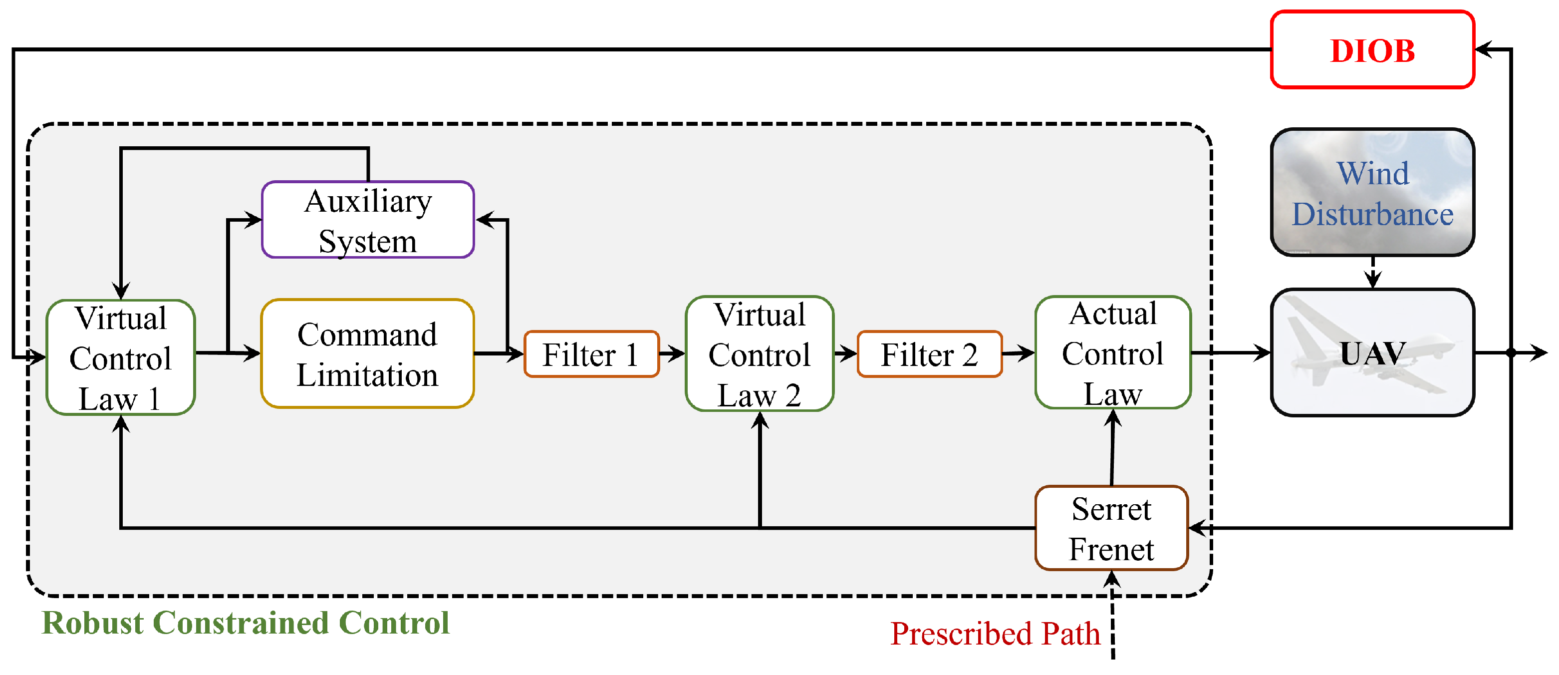
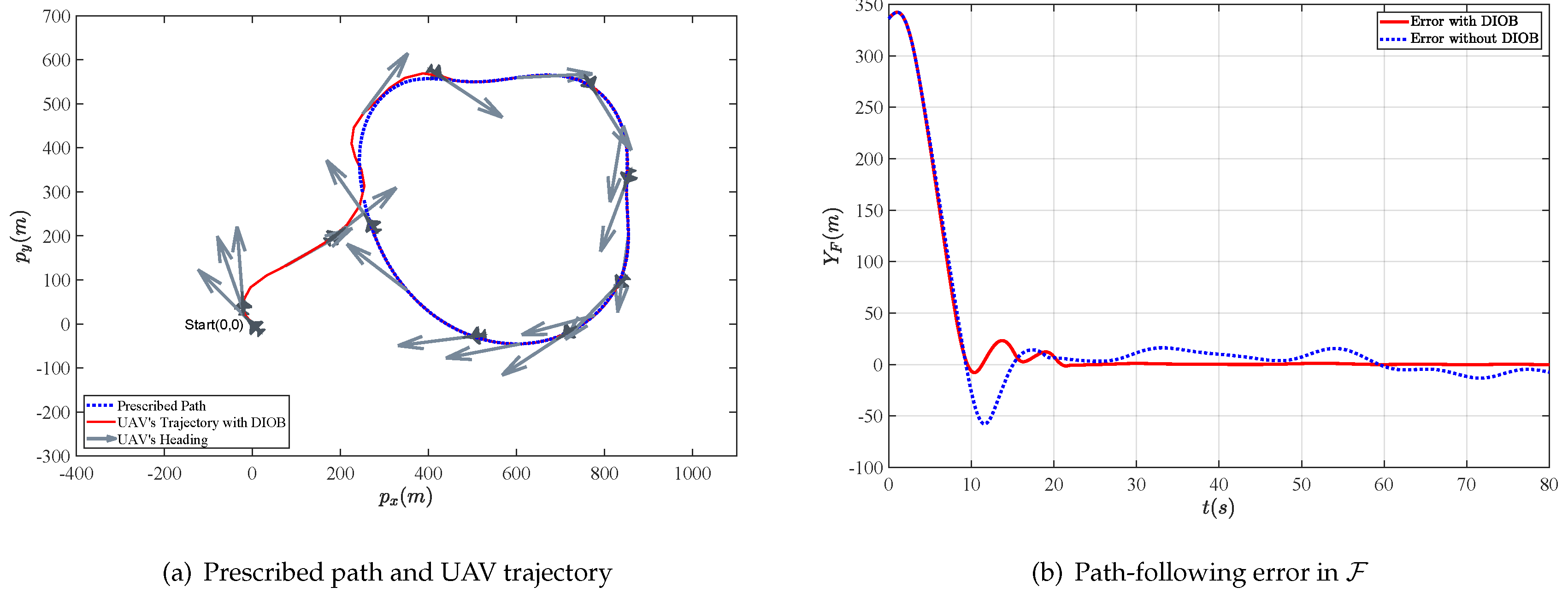
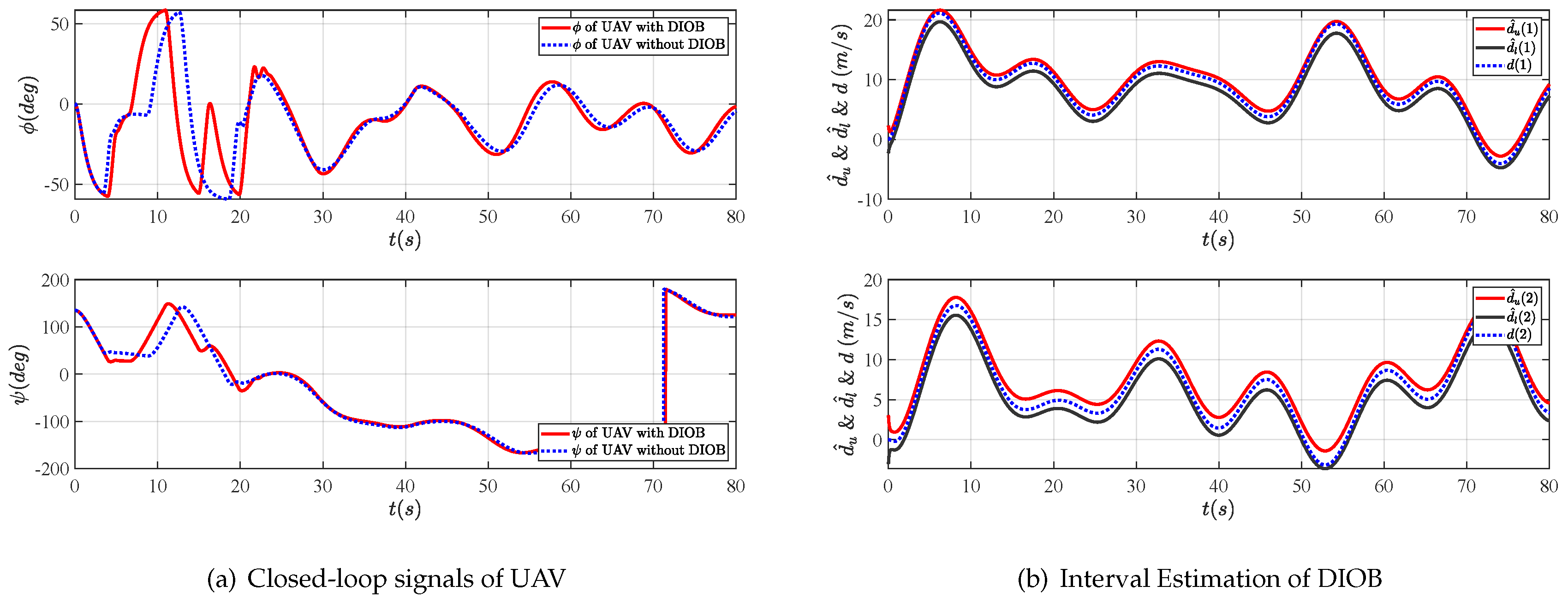
  • A specific DIOB is developed for the position kinematics of the UAV. Through the appropriate use of the information in the inertial framework, it is capable of providing interval estimation of the wind disturbances and providing more robustness for the feedforward compensation;
  • The Serret–Frenet frame is introduced to transform the path-following problem of the UAV into a general stabilizing control one. By improving the dynamic surface control technique, the resulting flight control design can address the non-affine nonlinearity of the UAV kinematics;
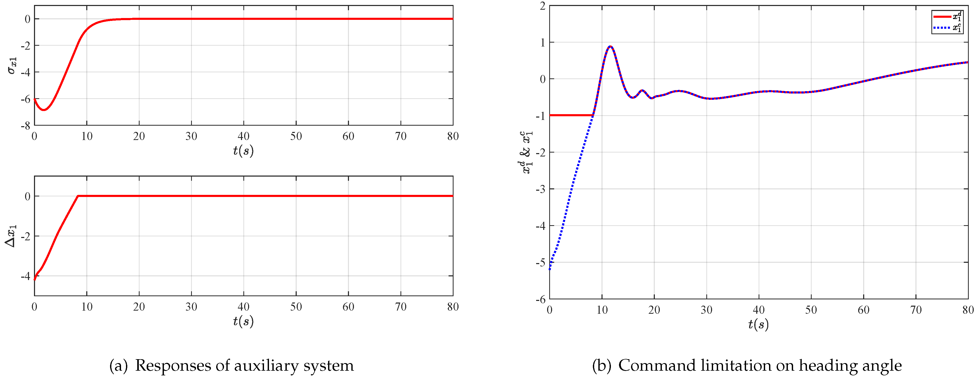
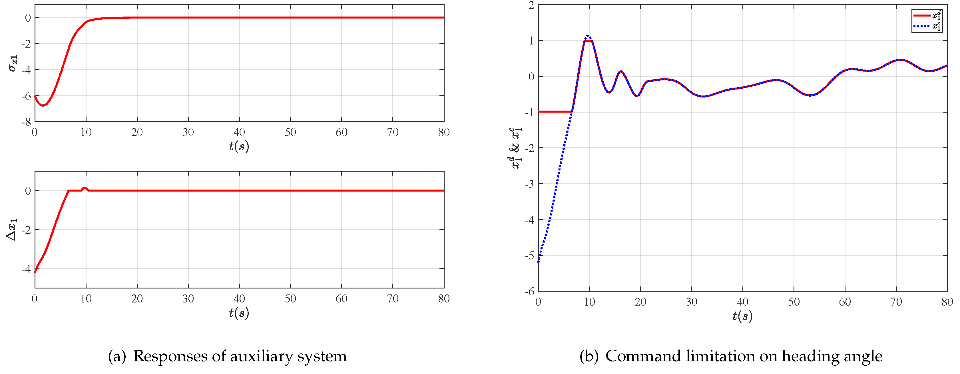
  • An auxiliary system is employed to address the command limitation on the heading angle of the UAV. Specifically, the stiff saturation nonlinearity is replaced with a saturation-like smooth nonlinear, which guarantees the differentiability of the virtual control law.
The structure of this paper is as follows: The second section describes the path-following problem of the UAV. The third section presents the design of the DIOB and the path-following control and then proves the stability of the closed-loop system. The fourth section verifies the effectiveness of this path-following method based on numerical simulations.
Symbol Description [2]:
  • R denotes the real number set, R n is an n-dimensional Euclidean space; meanwhile, R 0 = a n R | a n 0 and R > 0 = { a n R | a n > 0 } ;
  • For the given matrix or vector A n = [ A n i , j ] , define | A n | * = [ | A n i , j | ] , A n + = 0.5 ( A n + A n * ) and A n = A n + A n ;
  • For given matrices or vectors A n = [ A n i , j ] and B n = [ B n i , j ] , A n B n denotes that for any i , j have A n i , j B n i , j ;
  • For the given real symmetric matrix A n , A n 0 and A n 0 represent that the matrix A n is positive or negative definite, respectively;
  • For the given real symmetric matrix A n , λ max ( A n ) represents the maximum characteristic root of matrix A n ;
  • For the given matrix or vector A n , A n T denotes the transpose matrix of A n ;
  • For the given vector A n , | | A n | | denotes the Euclidean norm of A n .

2. Problem Formulation and Preliminaries

2.1. UAV Kinematics in Inertial Frame

This paper aims to solve the path-following problem of fixed-wing UAVs under wind disturbance. For convenience, only the kinematic model of the fixed-wing UAV is considered. At the same time, it is assumed that the UAV maintains a constant altitude and airspeed. Then, we obtain a suitable fixed-wing UAV kinematic model that is modeled in the inertial and body frames, i.e., I and B , as previously described [1,25].
p ˙ x = V a sin ψ + w x p ˙ y = V a cos ψ + w y ψ ˙ = g V a tan ϕ ϕ ˙ = b ϕ ( u ϕ )
where p x , p y R are the positions of the UAV in the inertial frame; V a is the airspeed; ψ R and ϕ R are the UAV’s heading and rolling angles, respectively; u R is the control input; w x R and w y R are the velocities of the wind disturbance in the inertial frame; b ϕ > 0 is a constant depending on the properties of the attitude controller; and g is the acceleration of gravity.
The variables involved in the kinematics (1) are shown in Figure 1, where x B , y B , and z B are the axes of the UAV body frame, O B is the coordinate origin of the body frame, and x I and y I are the axes of the inertial frame with P = [ p x , p y ] T .
In light of the existing modeling result [2], the wind disturbance d = [ w x , w y ] T is generated using the exogenous system as follows:
ω ˙ d = A ω ω d + B ω Δ ω ( t ) , d = C ω ω d
where ω d R m is the state of the exogenous system; A ω R m × m , B ω R 0 m × n and C ω R 0 2 × m are the known constant matrices with observable pair ( A ω , C ω ) and natural stable A ω ; Δ ω ( t ) R n is the unknown time-varying vector characterizing the modeling uncertainty of the wind disturbance; and m and n are two positive integers, which are the order of the system (2) related to the wind disturbance model established by the user. Regarding the properties of the wind disturbances, there exist oscillatory and damping modes for each direction of the wind disturbance. In the simulation part, we established a fourth-order system to simulate the wind disturbances in two different directions, namely m = 4 and n = 2 .

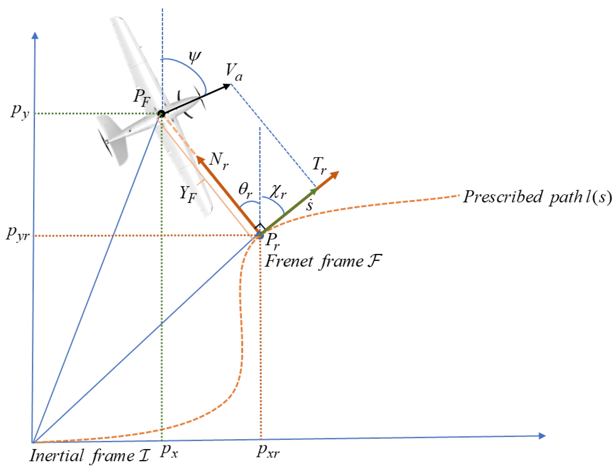
2.2. Path Following Based on the Serret–Frenet Frame

In terms of the path-following issue, we expect the position of the UAV to follow a prescribed path l ( s ) R 2 , which is a smooth curve determined by the length s. To transform the path-following issue into a general control problem, we introduce the Serret–Frenet frame F to redescribe the kinematic model of the UAV; the Serret–Frenet frame possesses more intuitions than the inertial one I on representing the positional relationship between the UAV and the prescribed path.
In Figure 2, a schematic diagram is presented to demonstrate the Serret–Frenet frame F , the inertial frame I , and the body frame B , where P r ( s ) = [ p x r ( s ) , p y r ( s ) ] T is the projection (reference) point of the UAV on the desired path l ( s ) . The Serret–Frenet frame is defined by the tangent vector ( T r ( s ) ) and the normal vector ( N r ( s ) ). Then, the coordinate of the UAV in F is given as P F = [ 0 , Y F ] T , where Y F is the vertical distance from the UAV to the reference point. Moreover, χ r is the desired path angle and θ r is the rotation angle between I and F . Thus, we have the following relations [39]:
χ ˙ r = θ ˙ r = ω c = k s ˙
where k is the curvature at the reference point P r ( s ) of the prescribed path, s ˙ is the speed of that on the prescribed path, and its specific form will be given later so in (11).
Based on the above Serret–Frenet Frame, the control objective is transformed to stabilize the distance from the UAV to the prescribed path, i.e., Y F 0 . According to Figure 2, the coordinate relationship between I and F is expressed as
P = P r + R F I P F
where R F I is the rotation matrix from F to I , and it has the following form [40]:
R F I = ( R I F ) T = cos θ r sin θ r sin θ r cos θ r
By using Rodrigues’ rotation formula [41], we obtain
d ( R F I P F ) d t = R F I d P F d t + R F I [ θ ˙ r ] × P F
with [ θ ˙ r ] × = 0 θ ˙ r θ ˙ r 0 .
By invoking (6), the derivative of P in (4) is written as follows: [40]:
d P d t I = d P r d t I + R F I d P F d t F + d R F I d t P F = d P r d t I + R F I d P F d t F + R F I 0 k s ˙ k s ˙ 0 P F
where ( ) I and ( ) F denote the coordinate representation of ∗ in the I frame and F frame, respectively.
By multiplying the rotation matrix R I F on both the left and right sides of (7), we obtain the dynamics of the path-following error P F in F as [40].
P ˙ F = R I F d P d t I R I F d P r d t I 0 k s ˙ k s ˙ 0 P F = R B F V a 0 + R I F w x w y R I F d P r d t I 0 k s ˙ k s ˙ 0 P F
where R B F is the rotation matrix from B to F as [40].
R B F = ( R F B ) T = cos ψ e sin ψ e sin ψ e cos ψ e
with ψ e = ψ χ r .
Finally, by expanding (8) and integrating (1), the dynamics of the path-following error in F is shown as
Y ˙ F = V a sin ψ e sin θ r w x + cos θ r w y ψ ˙ e = ψ ˙ χ ˙ r = g V a tan ϕ k s ˙ ϕ ˙ = b ϕ ( u ϕ )
and now, s ˙ denotes the moving speed of the reference point P r on the desired path, with the following form [40]:
s ˙ = V a cos ψ e / ( 1 k Y F )

2.3. Control Objective

With the path-following error dynamics (10), the control objective of this work is transformed to stabilize Y F by designing the control law for u.
To proceed with the control development, the following assumptions are made:
Assumption 1 
([38]). For the time-varying vector Δ ω ( t ) R n in the exogenous system (2), there exists a known constant vector Δ ¯ ω 0 n × 1 satisfying Δ ω ( t ) * Δ ¯ ω ;
Assumption 2 
([42]). Assume that ψ χ r is less than π 2 , ψ e < π 2 , which means ψ e = ψ e * when sin ψ e = sin ψ e * for any ψ e * < π 2 ;
Assumption 3 
([43]). The rolling angle of the UAV is less than π 2 , i.e., ϕ < π 2 , which indicates ϕ = ϕ * when tan ϕ = tan ϕ * for any ϕ * < π 2 ;
Assumption 4 
([42]). The infinite norm of wind d is less than UAV’s actual airspeed V a , which indicates | | d | | < V a for all t 0 .
Remark 1. 
The wind disturbance induced on the UAV should be bounded, and accordingly, for the states of the exogenous system. Moreover, there are abundant modeling results [2] based on the wind data to make A ω accurate. All these data make sure the boundedness of the modeling uncertainty Δ ω ( t ) and then the reasonability of Assumption 1.
Remark 2. 
The heading angle of the UAV is defined in ( π , π ] . The objective of path following is that the nose of the UAV adjusts to the desired orientation as quickly as possible. Therefore, the error of the course angle or heading angle is defined in [ 0 , π ] . The error can be converted to [ π / 2 , π / 2 ] by selecting a reasonable origin. Then, it is clear that Assumption 2 is rational.
Remark 3. 
In this work, we concentrate on the path-following control of the UAV. Of course, the normal flight situation of the UAV can accomplish the path-following objective. Thus, we only consider the normal flight situations of the UAV that do not include upside-down flying. Specifically, the roll angle of the UAV is within the range of [ π / 2 , π / 2 ] , which indicates Assumption 3 is reasonable.
Remark 4. 
Assumption 4 means that the wind resistance of the UAV is capable of being improved through controller design, while it is constrained by the physical performance of the UAV.
At the same time, for the design and use of DIOB, the following two lemmas are given:
Lemma 1 
([44]). For any given constant ϵ M > 0 and time-varying signal ϑ M , the inequality 0 ϑ M ϑ M tanh ( ϑ M ϵ M ) c M ϵ M always holds with c M = exp ( c M 1 ) = 0.2785 .
Lemma 2 
(Positive system, [45]). Suppose that there is a Metzler matrix K M R m × m (i.e., all its non-diagonal elements are non-negative.) and a non-negative time-varying vector Δ M ( t ) R 0 m , so that the system h ˙ M = K M h M + Δ M ( t ) has a unique solution for any initial state h M ( 0 ) R m . Then, given any initial state h M ( 0 ) R 0 m , it satisfies h M ( t ) R 0 m for any t > 0 .

3. Control Design and Stability Analysis

In this section, the DIOB is designed for the UAV kinematics in the inertial frame. The path-following control design is then presented based on the dynamic surface control technique and the auxiliary system is adopted to deal with the command limitation. Lastly, the stability analysis of the closed-loop system is presented.

3.1. Disturbance Interval Observer Design

In order to suppress the influence of wind disturbance on the UAV, a DIOB is introduced in this work. It will realize the interval estimation of the wind disturbance based on the nominal kinematics of the UAV in (1) and the known dynamics of the wind disturbance in (2).
For the simplicity of denotation, the position kinematics of the UAV in (1) is rewritten in the following vector form:
x ˙ p = f ( · ) + d
with x p = [ p x , p y ] T and f ( · ) = V a [ sin ψ , cos ψ ] T .
With the observer gain matrix L ω R m × 2 and the positive definite coordinate transformation matrix P ω R m × m , define intermediate variable z ω = P ω ( ω d L ω l ω ( x p ) ) and the function vector l ω ( x p ) = [ p x , p y ] T . By invoking (2) and (12), the dynamics of the intermediate variable z ω is obtained as follows [2]:
z ˙ ω = P ω A ω L ω C ω Q ω z ω + Θ ω + P ω B ω Δ ω ( t )
where Q ω is the inverse matrix of P ω , and they constitute the coordinate transformation for ( A ω L ω C ω ) , Θ ω is a known function vector with the following form:
Θ ω = P ω A ω L ω C ω L ω l ω ( x p ) P ω L ω l ω ( x p ) x p T f ( · )
Then, the interval observer is designed for the intermediate variable z ω , and the specific form of the DIOB is given by [2]
z ^ ˙ u = Γ ω z ^ u + Θ ω + P ω * B ω Δ ¯ ω z ^ ˙ l = Γ ω z ^ l + Θ ω P ω * B ω Δ ¯ ω d ^ u = C ω Q ω + z ^ u Q ω z ^ l + L ω l ω ( x p ) d ^ l = C ω Q ω + z ^ l Q ω z ^ u + L ω l ω ( x p )
where Γ ω = P ω A ω L ω C ω Q ω , z ^ u , z ^ l R m are the internal states of the DIOB and they constitute the interval estimate of the intermediate variable z ω , d ^ u , d ^ l R 2 are the outputs of the DIOB and they constitute the interval estimate of the wind disturbance d, and Δ ¯ ω is given in Assumption 1.
Define the estimation errors of the intermediate variable z ω as
z ˜ u = z ^ u z ω , z ˜ l = z ω z ^ l
and the variables of the wind disturbance d as
d ˜ u = d ^ u d , d ˜ l = d d ^ l
Then, we have the following lemma that summarizes the design condition of the DIOB:
Lemma 3 
(DIOB, [38]). For the UAV kinematic model (1) under the unknown wind disturbance generated by (2), design the DIOB according to (14):
  • If the designed matrices L ω and P ω make Γ ω be simultaneously Metzler and Hurwitz;
  • If the initial conditions of z ^ u and z ^ l satisfy z ^ l ( 0 ) z ω ( 0 ) z ^ u ( 0 ) .
Then, the estimation errors d ˜ l and d ˜ u of the DIOB are non-negative and bounded.
Proof of Lemma 3. 
By considering (13) and (14), the estimation errors z ˜ u and z ˜ l of intermediate variable z ω satisfy the following differential equations:
z ˜ ˙ u = Γ ω z ˜ u + P ω * B ω Δ ¯ ω P ω B ω Δ ω ( t ) z ˜ ˙ l = Γ ω z ˜ l + P ω * B ω Δ ¯ ω + P ω B ω Δ ω ( t )
According to the definition of B ω in (2), we know it satisfies B ω 0 m × n . According to Assumption 1, we further have P ω * B ω Δ ¯ ω P ω B ω Δ ω ( t ) P ω * B ω Δ ¯ ω . Based on Lemma 2, the design condition of Metzler matrix Γ ω , and the initial condition of z ^ l ( 0 ) z ω ( 0 ) z ^ u ( 0 ) , it is found that z ˜ u and z ˜ l are non-negative.
Define the interval width vector s ω = z ˜ u + z ˜ l for the intermediate variable z w . Since Γ ω is designed to be a Hurwitz matrix, there must be another matrix R ω 0 such that R ω Γ ω + Γ ω T R ω 0 . Define the Lyapunov function V ω = s ω T R ω s ω . By considering (15), it is found that the derivative of V ω satisfies the following inequality:
V ˙ ω = s ω T R ω ( z ˜ ˙ u + z ˜ ˙ l ) + ( z ˜ ˙ u + z ˜ ˙ l ) T R ω s ω = s ω T R ω ( Γ ω z ˜ u + Γ ω z ˜ l + 2 | P ω | * B ω Δ ¯ ω ) + ( Γ ω z ˜ u + Γ ω z ˜ l + 2 | P ω | * B ω Δ ¯ ω ) T R ω s ω = s ω T R ω Γ ω s ω + s ω T Γ ω T R ω s ω + 2 s ω T R ω ( | P ω | * B ω Δ ¯ ω ) + 2 ( | P ω | * B ω Δ ¯ ω ) T R ω s ω s ω T ( R ω Γ ω + Γ ω T R ω + 2 η ω R ω R ω ) s ω + | P ω | * B ω Δ ¯ ω 2 / η ω
where η ω > 0 is an adjustable parameter. It is known from R ω Γ ω + Γ ω T R ω 0 that there must be a suitable η ω to make R ω Γ ω + Γ ω T R ω + 2 η ω R ω R ω 0 which indicates that the interval width vector s ω is bounded. Furthermore, because of the non-negative characteristics of z ˜ u and z ˜ l , we obtain that z ˜ u and z ˜ l are also bounded.
Consider the definitions of estimation errors d ˜ u and d ˜ l , and they satisfy the following equations:
d ˜ u = d ^ u d = C ω ( Q ω + z ˜ u + Q ω z ˜ l ) , d ˜ l = d d ^ l = C ω ( Q ω + z ˜ l + Q ω z ˜ u )
Finally, we can conclude that d ˜ l and d ˜ u are non-negative and bounded. This completes the proof. □

3.2. Robust Constrained Control Design

At this stage, the robust constrained control law is designed for the path-following error dynamics (10). Before presenting the control design, a block diagram of the closed-loop system is shown in Figure 3. It is seen from Figure 3 that the block “UAV” is the actual plant. The block “Serret–Frenet transformation” is used to calculate the path-following error in the Serret–Frenet frame. The block “DIOB” generates wind disturbance estimation for “Virtual Control Law 1”. The designed control follows the dynamic surface technique. Specifically, two virtual control laws, i.e., “Virtual Control Law 1” and “Virtual Control Law 2”, and a control law, i.e., “actual control law”, are designed. In order to avoid the differential explosion issue, two filters, i.e., “Filter 1” and “Filter 2”, are introduced to obtain the deviations of the virtual control laws. Moreover, the "auxiliary system” is employed to solve the instability problem caused by “command limitation”.
The control design follows a step-by-step procedure.
Step 1: For the convenience of symbol use, let
[ w ^ x , w ^ y ] T = d ^ = 0.5 ( d ^ u + d ^ l ) , [ w ¯ x , w ¯ y ] T = d ¯ = 0.5 ( d ^ u d ^ l )
represent the middle-value vector and the weight vector of the DIOB, respectively. In the controller design process, we use d ^ and d ¯ as the compensation and robust terms, respectively.
Define path-following error e Y = Y F . According to the controller design goal, i.e., e Y 0 , we design a positive definite function about e Y to measure the energy of the system tracking error. According to the general Lyapunov function design method, we select the following positive definite quadratic function:
V 0 = 1 2 k 1 e Y 2
where k 1 > 0 is a tuning parameter to be designed.
By considering the path-following error dynamics (10), the differential form of V 0 is written as
V ˙ 0 = k 1 e Y ( V a sin ψ e sin θ r w x + cos θ r w y )
To overcome the non-affine non-linearity of sin ( · ) , we directly design the virtual control law x 1 d [ 1 , 1 ] for “ sin ψ e ”. In light of the natural bounded characteristic of sin ( · ) , the virtual control law x 1 d undergoes the following command limitation:
x 1 d = ( γ τ + ( 1 γ ) τ tanh | x 1 c | / τ γ 1 γ ) sign ( x 1 c ) | x 1 c | > γ τ x 1 c | x 1 c | γ τ
where x 1 c is the nominally designed virtual control law of “ sin ψ e ” without considering the command limitation, and 0 < γ < 1 and τ > 0 are the adjustable parameter and the amplitude of limitation, respectively.
In order to avoid the instability of the control system caused by the command limitation (20), an auxiliary system is constructed as [46]
σ ˙ x 1 = k σ σ x 1 1 σ x 1 ( | k 1 V a e Y Δ x 1 | + Δ x 1 2 2 ) + Δ x 1 | σ x 1 | > μ 0 | σ x 1 | μ
where Δ x 1 = x 1 c x 1 d , σ x 1 R is the state of the auxiliary system, k σ > 0 is the parameter to be designed, and μ is a positive tuning number which should be appropriately selected according to the system performance requirement.
Then, design the virtual control law x 1 c as follows:
x 1 c = c 1 e Y V a + w ¯ x sin θ r e Y V a tanh sin θ r e Y ϵ 1 + w ¯ y cos θ r e Y V a tanh cos θ r e Y ϵ 1 + w ^ x sin θ r w ^ y cos θ r V a σ x 1
where c 1 > 0 is the feedback gain and ϵ 1 > 0 is a tuning parameter.
Meanwhile, in order to avoid the complexity explosion problem, a filter variable x 2 f R is introduced. The form of the low-pass filter is given as follows [47]:
ω 1 x ˙ 2 f + x 2 f = x 1 d , x 2 f ( 0 ) = x 1 d ( 0 )
where ω 1 > 0 is the time constant of the filter to be designed.
Define the tracking error e 2 = sin ψ e x 2 f for sin ψ e and the estimation error of the low-pass filter as
δ 1 = x 2 f x 1 d
Substituting (22) and (23) into (19) yields
V ˙ 0 = k 1 e Y ( V a ( e 2 + x 2 f ) sin θ r w x + cos θ r w y ) = k 1 e Y ( V a ( e 2 + x 1 d + δ 1 ) sin θ r w x + cos θ r w y ) = k 1 e Y ( V a ( e 2 Δ x 1 + x 1 c + δ 1 ) sin θ r w x + cos θ r w y ) = c 1 k 1 e Y 2 + k 1 V a e Y ( e 2 + δ 1 ) k 1 e Y sin θ r w ˜ x + k 1 e Y cos θ r w ˜ y k 1 e Y sin θ r tanh ( sin θ r e Y / ϵ 1 ) w ¯ x k 1 cos θ r e Y tanh ( cos θ r e Y / ϵ 1 ) w ¯ y k 1 V a e Y Δ x 1 k 1 V a e Y σ x 1
where [ w ˜ x , w ˜ y ] T = d ˜ = d d ^ = [ w ^ x w x , w ^ y w y ] T .
According to the interval property of the DIOB in Lemma 3, we have
d ˜ u = d ^ u d 0 , d ˜ l = d d ^ l 0
and then,
d ¯ d ˜ = 0.5 ( d ^ u d ^ l ) ( d 0.5 ( d u ^ + d ^ l ) ) = d ^ u d 0 d ¯ + d ˜ = 0.5 ( d ^ u d ^ l ) + ( d 0.5 ( d u ^ + d ^ l ) ) = d d ^ l 0
which indicates d ¯ | d ˜ | , namely,
| w ˜ x | w ¯ x , | w ˜ y | w ¯ y
In light of Lemma 1, we further have
e Y sin θ r w ˜ x sin θ r e Y w ¯ x sin θ r e Y tanh ( sin θ r e Y / ϵ 1 ) w ¯ x + ϵ 1 w ¯ x e Y cos θ r w ˜ y cos θ r e Y w ¯ y cos θ r e Y tanh ( cos θ r e Y / ϵ 1 ) w ¯ y + ϵ 1 w ¯ y
By considering (25) and (27), we have
V ˙ 0 c 1 k 1 e Y 2 + k 1 V a e Y ( e 2 + δ 1 ) + k 1 e Y sin θ r w ˜ x k 1 V a e Y Δ x 1 k 1 V a e Y σ x 1 k 1 sin θ r e Y tanh s i n θ r e Y ϵ 1 w ¯ x + k 1 e Y cos θ r w ˜ y k 1 cos θ r e Y tanh cos θ r e Y ϵ 1 w ¯ y c 1 k 1 e Y 2 + k 1 V a e Y ( e 2 + δ 1 ) + k 1 ϵ 1 w ¯ x + k 1 ϵ 1 w ¯ y k 1 V a e Y Δ x 1 k 1 V a e Y σ x 1
Define the positive function V 1 as
V 1 = V 0 + 1 2 σ x 1 2 = 1 2 k 1 e Y 2 + 1 2 σ x 1 2
Considering the situation when saturation occurs, and invoking (18) and (28), we have the derivative form of V 1 as follows:
V ˙ 1 c 1 k 1 e Y 2 + k 1 V a e Y ( e 2 + δ 1 ) + k 1 ϵ 1 w ¯ x + k 1 ϵ 1 w ¯ y k 1 V a e Y Δ x 1 k 1 V a e Y σ x 1 + σ x 1 ( k σ σ x 1 1 σ x 1 ( | k 1 V a e Y Δ x 1 | + Δ x 1 2 2 ) + Δ x 1 ) = c 1 k 1 e Y 2 + k 1 V a e Y ( e 2 + δ 1 ) + k 1 ϵ 1 w ¯ x + k 1 ϵ 1 w ¯ y k 1 V a e Y Δ x 1 k 1 V a e Y σ x 1 k σ σ x 1 2 | k 1 V a e Y Δ x 1 | Δ x 1 2 2 + σ x 1 Δ x 1
By using Young’s inequality, we have
σ x 1 Δ x 1 1 2 σ x 1 2 + 1 2 Δ x 1 2
With further consideration of (30) and (31), we obtain
V ˙ 1 c 1 k 1 e Y 2 + k 1 V a e Y ( e 2 + δ 1 ) + k 1 ϵ 1 w ¯ x + k 1 ϵ 1 w ¯ y k 1 V a e Y Δ x 1 k 1 V a e Y σ x 1 k σ σ x 1 2 | k 1 V a e Y Δ x 1 | + σ x 1 2 2
Because of k 1 V a e Y Δ x 1 | k 1 V a e Y Δ x 1 | 0 , we can reduce inequality (32) as
V ˙ 1 c 1 k 1 e Y 2 + k 1 V a e Y ( e 2 + δ 1 ) + k 1 ϵ 1 ( w ¯ x + w ¯ y ) k 1 V a e Y σ x 1 + ( 1 2 k σ ) σ x 1 2
Considering the situation when saturation does not occur, the state of the auxiliary system satisfies σ x 1 = 0 . We have the derivative form of V 1 as follows:
V ˙ 1 c 1 k 1 e Y 2 + k 1 V a e Y ( e 2 + δ 1 ) + k 1 ϵ 1 w ¯ x + k 1 ϵ 1 w ¯ y
Step 2: Define a Lyapunov function candidate V 2 as
V 2 = 1 2 k 2 e 2 2
where k 2 > 0 is an adjustable parameter.
To design the next virtual control law, the differential form of V 2 is written as
V ˙ 2 = k 2 e 2 ( cos ψ e ψ ˙ e + δ 1 ω 1 )
By invoking (10), we obtain
V ˙ 2 = k 2 e 2 cos ψ e ( g V a tan ϕ k s ˙ ) + δ 1 ω 1
Then, we design the virtual control law for “ tan ϕ ” as
x 2 d = V a k s ˙ g V a ( c 2 e 2 + k 1 k 2 V a e Y ) g cos ψ e
where c 2 > 0 is the feedback gain, and cos ψ e is always positive under Assumption 2.
Process x 2 d in the same way as x 1 d and design low-pass filter as [47]
ω 2 x ˙ 3 f + x 3 f = x 2 d , x 3 f ( 0 ) = x 2 d ( 0 )
where x 3 f R is the filter variable, and ω 2 > 0 is the time constant of the filter. Accordingly, the estimation error of the low-pass filter (39) is defined as
δ 2 = x 3 f x 2 d
According to Assumption 3, define tracking error of virtual control law as e 3 = tan ϕ x 3 f . By using (38), the derivative of V 2 is rewritten as
V ˙ 2 = k 2 e 2 cos ψ e ( g V a ( e 3 + x 3 f ) k s ˙ ) + δ 1 ω 1
By using (40), we obtain the following derivative form of V 2 :
V ˙ 2 = k 2 e 2 cos ψ e ( g V a ( e 3 + x 2 d + δ 2 ) k s ˙ ) + δ 1 ω 1 = c 2 k 2 e 2 2 + k 2 e 2 cos ψ e g V a δ 2 + k 2 e 2 e 3 cos ψ e g V a + k 2 e 2 δ 1 ω 1 k 1 V a e Y e 2
Step 3: Choose another Lyapunov function candidate V 3 as
V 3 = 1 2 k 3 e 3 2
where k 3 > 0 is an adjustable parameter.
By invoking (10), the differential from of V 3 is shown as
V ˙ 3 = k 3 e 3 ( ϕ ˙ sec 2 ϕ x ˙ 3 f )
Using (39), we have the following inequality:
V ˙ 3 = k 3 e 3 ( sec 2 ϕ ) b ϕ ( u ϕ ) + δ 2 ω 2
Thus, we design the nominal control law u as
u = ϕ + cos 2 ϕ b ϕ c 3 e 3 k 2 k 3 e 2 cos ψ e g V a
where c 3 > 0 is the feedback gain.
Substituting the control law (46) into (45) yields
V ˙ 3 = c 3 k 3 e 3 2 + k 3 e 3 δ 2 ω 2 k 2 e 2 e 3 cos ψ e g V a

3.3. Stability Analysis
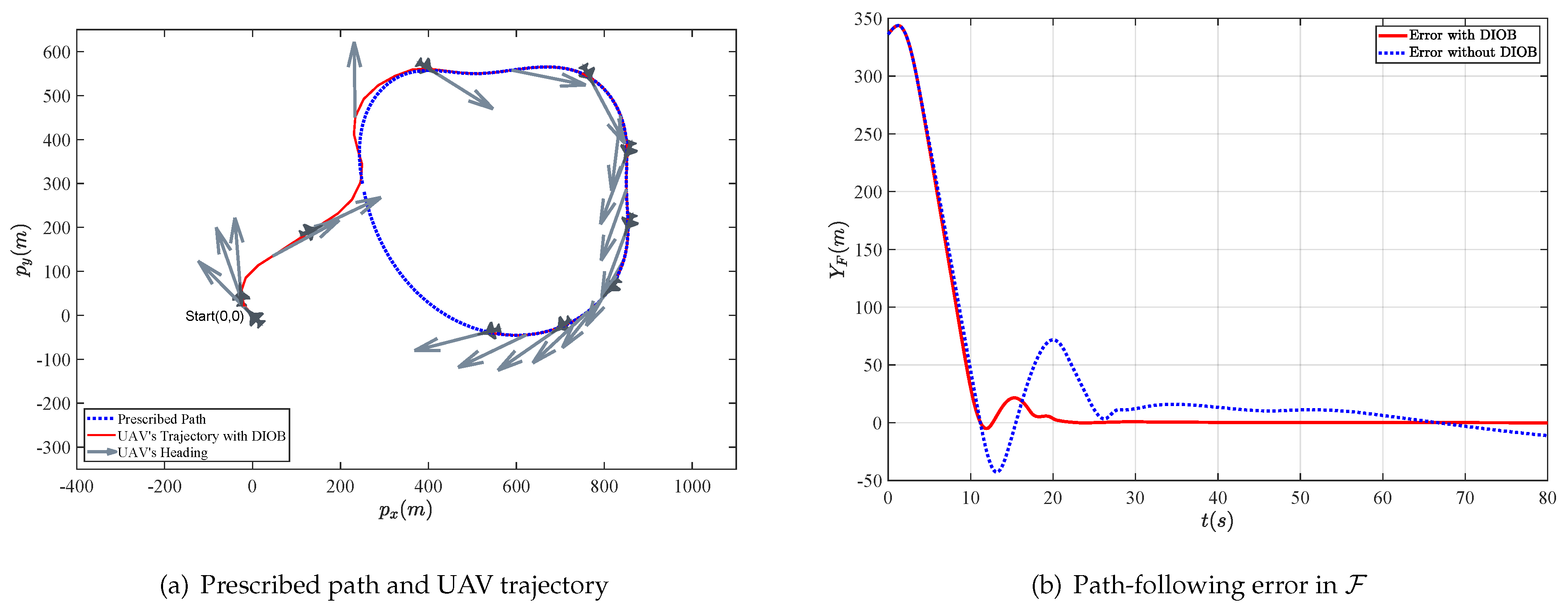
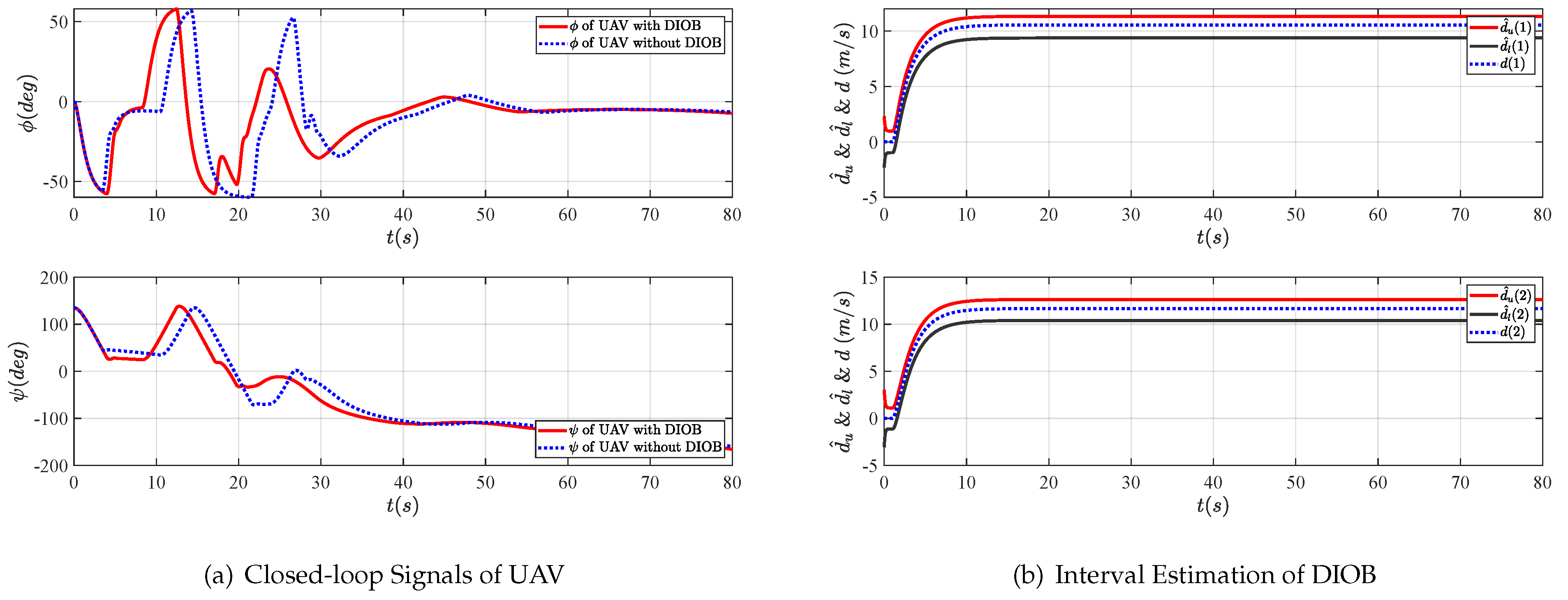
Theorem 1. 
For the kinematics model (1) of the UAV, consider the wind disturbance is generated by using (2). Design the DIOB according to Lemma 3. Based on the filter (23), (39), and the auxiliary system (21), design the virtual control law (22) and (38), and control law (46) for the path-following error dynamics (10). With any given parameters γ, τ, μ, η ω , and η ϵ , if the matrices R ω , P ω , Q ω , L ω , the feedback gains c 1 , c 2 , c 3 , filters’ parameters ω 1 , ω 2 , and the tuning parameters k 1 , k 2 , k 3 , k σ satisfy the following linear matrix inequalities:
Ξ C 0 Ξ D 0
where Ξ C and Ξ D have the following forms:
Ξ C = c 1 k 1 0 1 × 1 0 1 × 1 k 1 V a / 2 0 1 × 1 0.5 k 1 V a 0 1 × 1 c 2 k 2 0 1 × 1 k 2 / ( 2 ω 1 ) k 2 g / ( 2 V a ) 0 1 × 1 0 1 × 1 0 1 × 1 c 3 k 3 k 3 / ( 2 ω 2 ) 0 1 × 1 0 1 × 1 k 1 V a / 2 k 2 / ( 2 ω 1 ) k 3 / ( 2 ω 2 ) 1 / ω 1 0 1 × 1 0 1 × 1 0 1 × 1 k 2 g / ( 2 V a ) 0 1 × 1 0 1 × 1 1 / ω 2 0 1 × 1 0.5 k 1 V a 0 1 × 1 0 1 × 1 0 1 × 1 0 1 × 1 0.5 k σ Ξ D = R ω Γ ω + Γ ω T R ω + η ϵ I m * * R ω 0.5 / η ω * Λ 0 1 × 1 1 / ( k 1 ϵ 1 η ϵ )
with Λ = [ 1 , 1 ] C ω | Q ω | * , then the UAV can stably follow the prescribed path.
Proof of Theorem 1. 
Firstly, we analyze the error of the low-pass filter contained in (23). From (20) and (22), we know that there exists a constant x ¯ 1 d > 0 such that | x ˙ 1 d | x ¯ 1 d . By using (23) and (24), we obtain
δ ˙ 1 = x ˙ 2 f x ˙ 1 d = x 1 d x 2 f ω 1 x ˙ 1 d = 1 ω 1 δ 1 x ˙ 1 d 1 ω 1 δ 1 + x ¯ 1 d
By solving the differential equation, we have
δ 1 ( δ 1 ( 0 ) ω 1 x ¯ 1 d ) e t ω + ω 1 x ¯ 1 d
Obviously, there is a constant δ ¯ 1 > 0 that makes δ 1 δ ¯ 1 . Similarly, there are constants δ ¯ 2 > 0 and x ¯ 2 d > 0 that makes δ 2 δ ¯ 2 and | x ˙ 2 d | x ¯ 2 d .
Define a positive function as
V 4 = V 1 + V 2 + V 3 + V ω + 0.5 δ 1 2 + 0.5 δ 2 2 = 0.5 k 1 e Y 2 + 0.5 k 2 e 2 2 + 0.5 k 3 e 3 2 + 0.5 δ 1 2 + 0.5 δ 2 2 + s ω T R ω s ω + 0.5 σ x 1 2
By using (16), (33), (42), and (47), we have the following derivative form of V 4 :
V ˙ 4 = V ˙ 1 + V ˙ 2 + V ˙ 3 + V ˙ ω + δ 1 δ ˙ 1 + δ 2 δ ˙ 2 c 1 k 1 e Y 2 c 2 k 2 e 2 2 c 3 k 3 e 3 2 + k 1 V a e Y δ 1 + k 2 g V a e 2 δ 2 + k 2 ω 1 e 2 δ 1 + ( 1 2 k σ ) σ x 1 2 + k 3 ω 2 e 3 δ 2 + k 1 ϵ 1 ( w ¯ x + w ¯ y ) δ 1 2 ω 1 + δ ¯ 1 x ¯ 1 d δ 2 2 ω 2 + δ ¯ 2 x ¯ 2 d k 1 V a e Y σ x 1 + s ω T ( R ω Γ ω + Γ ω T R ω + 2 η ω R ω R ω ) s ω + | P ω | * B ω Δ ¯ ω 2 / η ω
After combining the DIOB in (17), we obtain w ¯ x + w ¯ y = [ 1 , 1 ] d ¯ = [ 1 , 1 ] C ω | Q ω | * s ω . The inequality (52) is written as
V ˙ 4 c 1 k 1 e Y 2 c 2 k 2 e 2 2 c 3 k 3 e 3 2 + k 1 V a e Y δ 1 + k 2 g V a e 2 δ 2 + k 2 ω 1 e 2 δ 1 + ( 1 2 k σ ) σ x 1 2 + k 3 ω 2 e 3 δ 2 + [ 1 , 1 ] k 1 ϵ 1 C ω | Q ω | * s ω δ 1 2 ω 1 + δ ¯ 1 x ¯ 1 d δ 2 2 ω 2 + δ ¯ 2 x ¯ 2 d k 1 V a e Y σ x 1 + s ω T ( R ω Γ ω + Γ ω T R ω + 2 η ω R ω R ω ) s ω + | P ω | * B ω Δ ¯ ω 2 / η ω λ max ( Ξ C , Ξ D ) V 4 + δ ¯ 1 x ¯ 1 d + δ ¯ 2 x ¯ 2 d + | P ω | * B ω Δ ¯ ω 2 / η ω
By further considering (48), we can scale inequality (53) as
V ˙ 4 a V 4 + b
where a = λ max ( Ξ C , Ξ D ) and b = δ ¯ 1 x ¯ 1 d + δ ¯ 2 x ¯ 2 d + | P ω | * B ω Δ ¯ ω 2 / η ω .
By solving the differential equation, the following inequality is obtained:
V 4 ( V 4 ( 0 ) b a ) e a t + b a , t 0
When matrix Ξ C and Ξ D are negative, a = λ max ( Ξ C , Ξ D ) > 0 , we obtain
V 4 b a , ( t )
According to the definition of V 4 in (51) and inequality (52), we know that by choosing appropriate parameters, the path-following error finally converges to a neighborhood of the origin. This completes the proof. □
In view of the many design parameters of the above control scheme, the feasibility of the controller is analyzed in combination with the stability condition (48), and the influence of the parameter design on the performance of the closed-loop system is summarized as follows: Considering the unit and order of magnitude, the value of k 1 should be far less than k 2 and k 3 . Since the pair ( A ω , C ω ) satisfies the observable condition, there always exists an observer gain matrix L ω satisfying the stability condition (48) for any given ϵ 1 . The controller parameters c 1 , c 2 , and c 3 are the feedback gains of the controller, which determine the response speed of each loop. From the practical insight of the UAV, the response speed of ϕ is greater than ψ e , and the response speed of ψ e is faster than Y F . Nevertheless, once c 3 is too large, it will increase the burden of the UAV attitude loop. The smaller the filter coefficients ω 1 and ω 2 , the smaller the filtering error. However, this will cause the system to overshoot.
Remark 5. 
The proposed method using active anti-disturbance technology possesses more anti-disturbance capability compared with the classical robust methods such as those developed in previous studies [20,39,48]. The disturbance estimation would also provide freedom for users to select control gains. Meanwhile, compared with previous trajectory-tracking methods [3,4,28], the proposed path-following method eliminates the speed constraint and provides convenience for the speed control of the fixed-wing UAV.

4. Simulations

In this section, we provide the simulation results to verify the effectiveness of the path-following strategy based on the DIOB. The prescribed path-generation method is not the focus of this paper (the specific method can be found in [49]), and the UAV parameters used in the simulation were defined according to [1].
In terms of (2), we designed the system matrix A ω , the input matrix B ω , and the output matrix C ω of the exogenous system. Considering the dynamics of the wind disturbance, there were oscillatory and damping modes for each direction of the wind disturbance. Therefore, we used a fourth-order system to simulate the disturbances in two different directions simultaneously, and a second-order system simulated the wind disturbances in each direction. The poles of the system were configured at [ 0.48251 , 2.000 ± 1.414 i , 3.517 ] . Furthermore, taking into account the coupling effect of the two directions of disturbance, the matrix of the exogenous system was designed as follows:
A ω = 0 1 0 0 3 4 1 0 0 1 0 1 0 0 3 4 , B ω = 0 0 1 0 0 0 0 1 , C ω = 1 0 0 0 0 0 1 0
According to Section 3.1, the parameters of the DIOB were selected as
L ω = 16.2614 0.0949 34.5782 0.4160 0.0896 16.3386 37.0269 34.4678 , P ω = 371.3692 18.0876 262.8437 43.8073 39.4641 16.2636 59.7440 9.7941 388.2665 23.7900 240.7687 38.8337 23.5667 9.5612 36.6690 5.8205
The control gains in the DIOB-based path-following control law in Section 3.2 were selected as c 1 = 1 , c 2 = 5 , c 3 = 8 . The parameters of filters were selected as ω 1 = 1 , ω 2 = 1 . The parameters of the auxiliary system were selected as k σ = 0.5 , μ = 0.1 . The purpose of this scenario was to drive the UAV to follow an irregular path. The speed of the UAV was kept at a constant 30 m/s. The UAV was started from location ( 0 , 0 ) . In this section, three different types of disturbances are analyzed for simulation verification.
Case 1 (Step Wind Disturbances): The inputs of the exogenous system (2) are step signals, which are used to simulate the continuous constant wind disturbance of UAV. The path-following performance is shown in Figure 4a. It shows that the controller can stably follow the prescribed path. To clearly show the difference, we show the path-following error in the F frame in Figure 4b. The UAV with the DIOB-based path-following controller can follow the prescribed path faster and more stably. Moreover, the steady-state path-following error is smaller than the UAV without the DIOB controller. Figure 5a shows the heading angle and the roll angle of the UAV. The estimation errors of DIOB are shown in Figure 5b. Figure 6 shows the state of the auxiliary system, the virtual control law x 1 d , and so on. We see that command x 1 d is saturated before 9 s, which changes the state σ x 1 of the auxiliary system.
Case 2 (Sinusoidal Wind Disturbances): The inputs of the exogenous system (2) are sinusoidal signals. Compared with case 1, the disturbance signals are multi-frequency sinusoidal signal combinations. This case simulates the dynamic disturbance of UAV during flight. The path-following performance and path-following error in F are shown in Figure 7a,b, respectively. The path-following performance of the UAV did not change significantly. The UAV could still follow the prescribed path stably, quickly, and accurately. Figure 8a,b show the heading angle and the roll angle of the UAV and the outputs of the DIOB. The state of auxiliary and the virtual control law x 1 d and x 1 c are shown in Figure 9. Two times of saturation occurred in 0–5 s and about 10 seconds, respectively. The auxiliary system effectively enhanced the stability of the closed-loop system under the command limitation.
Case 3 (Comparison Study): To show the proposed method’s characteristics more intuitively, we selected a more complicated path for simulation research. In addition, for this case, we selected some common path-following methods for comparative study, including the VTP based on the geometric method, the LQI, and the classical disturbance observer-based control (DOBC). In the simulation, we used the motion model proposed in (1) uniformly. The wind disturbance, in this case, was the same as that in case 2. Figure 10 shows the tracking and following error comparison of the different methods. It can be seen from Figure 10a that the four methods used could stably follow the reference path. Figure 10b shows a clear comparison of the path-following error of the various methods. In the wind disturbance environment, the effect of the VTP method was the worst, closely followed by the LQI. Obviously, in this scenario, the DOBC method and DIOB method were better than the former two methods. Since both the DIOB and DOBC use the estimated disturbance information as feedforward control, their performance was very close. However, we can see that the anti-disturbance ability of the DIOB method was slightly better than that of the DOBC, as shown in Figure 10b.
In order to show the performance of various methods more intuitively, we selected two performance indexes for comparison. One is the integration of the absolute value of the error Δ e r r o r = 0 t e n d | Y F | d t , and the other is the integration of the absolute value of the system input Δ u = 0 t e n d | u | d t , where t e n d is the end time of the simulation. Δ e r r o r measures the path-following error, and Δ u measures the energy consumption of the system. The performance indexes of case 3 are shown in Table 1. It can be seen that, in this case, the error indexes of the DIOB method and the DOBC method schemes were far less than the other two, and the energy consumption of the DIOB method was slightly less than that of the DOBC method.
Overall, the path-following control method of UAVs based on the DIOB can address various forms of external disturbances and different forms of reference paths. Compared with the general path-following control strategy, it shows better path-following performance in the specific situation.

5. Summary

In this work, we presented the robust constrained path-following control scheme for UAVs under wind disturbances. By appointing the projection from the UAV to the path, the Serret–Frenet frame was introduced, and the complexity of the path-following problem was reduced. Specifically, the DIOB was employed, and it proved capable of generating the upper and lower boundaries of the wind disturbances. The path-following control design was presented based on the dynamic surface control technique, and the auxiliary system was adopted to address the command limitation. Theoretical analysis revealed the design conditions and feasibility endurance. The effectiveness of the developed control scheme was demonstrated with numerical simulations. It is worth highlighting that there are still many unexplored research avenues for the path-following problem in UAVs. For example, the 3 or 4 dimensional path-following control methods of UAVs should be taken into consideration in the future. The modeling for wind disturbance in this paper is relatively simple. In addition, the UAV path-following control under random wind disturbance is still a challenge.

Author Contributions

Methodology, Y.S. and K.Y.; writing—original draft preparation, Y.S.; writing—review and editing, K.Y. and Y.S.; validation, Y.S. and X.W. All authors have read and agreed to the published version of the manuscript.

Funding

This work was supported in part by the Natural Science Foundation of Jiangsu Province under Grant BK20210284, in part by the National Natural Science Foundation of China under Grant 62103188, and in part by International Postdoctoral Exchange Fellowship Program under Grant PC2022031.

Data Availability Statement

Not applicable.

Conflicts of Interest

The authors declare no conflict of interest.

References

  1. Beard, R.W.; McLain, T.W. Small Unmanned Aircraft: Theory and Practice; Princeton University Press: Princeton, NJ, USA, 2012. [Google Scholar]
  2. Yong, K. Disturbance interval observer-based carrier landing control of unmanned aerial vehicles using prescribed performance. Sci. Sin. Informationis 2022, 52, 1711. [Google Scholar] [CrossRef]
  3. Chen, M.; Xiong, S.; Wu, Q. Tracking flight control of quadrotor based on disturbance observer. IEEE Trans. Syst. Man Cybern. Syst. 2019, 51, 1414–1423. [Google Scholar] [CrossRef]
  4. Ye, H.; Chen, M.; Zeng, Q. Horizontal motion tracking control for an underwater vehicle with environmental disturbances. In Proceedings of the 2017 36th Chinese Control Conference (CCC), Dalian, China, 26–28 July 2017; pp. 4952–4957. [Google Scholar] [CrossRef]
  5. Yong, K.; Chen, M.; Wu, Q. Immersion and invariance-based integrated guidance and control for unmanned aerial vehicle path following. Int. J. Syst. Sci. 2019, 50, 1052–1068. [Google Scholar] [CrossRef]
  6. Beard, R.W.; Ferrin, J.; Humpherys, J. Fixed wing UAV path following in wind with input constraints. IEEE Trans. Control. Syst. Technol. 2014, 22, 2103–2117. [Google Scholar] [CrossRef]
  7. Aguiar, A.P.; Hespanha, J.P.; Kokotovic, P.V. Path-following for nonminimum phase systems removes performance limitations. IEEE Trans. Autom. Control 2005, 50, 234–239. [Google Scholar] [CrossRef] [Green Version]
  8. Aguiar, A.P.; Hespanha, J.P. Trajectory-tracking and path-following of underactuated autonomous vehicles with parametric modeling uncertainty. IEEE Trans. Autom. Control 2007, 52, 1362–1379. [Google Scholar] [CrossRef] [Green Version]
  9. Park, S.; Deyst, J.; How, J.P. Performance and lyapunov stability of a nonlinear path following guidance method. J. Guid. Control Dyn. 2007, 30, 1718–1728. [Google Scholar] [CrossRef]
  10. Kaminer, I.; Pascoal, A.; Xargay, E.; Hovakimyan, N.; Cao, C.; Dobrokhodov, V. Path following for small unmanned aerial vehicles using L1 adaptive augmentation of commercial autopilots. J. Guid. Control Dyn. 2010, 33, 550–564. [Google Scholar] [CrossRef] [Green Version]
  11. Nelson, D.R.; Barber, D.B.; McLain, T.W.; Beard, R.W. Vector field path following for miniature air vehicles. IEEE Trans. Robot. 2007, 23, 519–529. [Google Scholar] [CrossRef] [Green Version]
  12. Chen, H.; Chang, K.; Agate, C.S. UAV path planning with tangent-plus-Lyapunov vector field guidance and obstacle avoidance. IEEE Trans. Aerosp. Electron. Syst. 2013, 49, 840–856. [Google Scholar] [CrossRef]
  13. Frew, E.W.; Lawrence, D. Tracking dynamic star curves using guidance vector fields. J. Guid. Control Dyn. 2017, 40, 1488–1495. [Google Scholar] [CrossRef]
  14. Xargay, E.; Kaminer, I.; Pascoal, A.; Hovakimyan, N.; Dobrokhodov, V.; Cichella, V.; Aguiar, A.P.; Ghabcheloo, R. Time-critical cooperative path following of multiple unmanned aerial vehicles over time-varying networks. J. Guid. Control Dyn. 2013, 36, 499–516. [Google Scholar] [CrossRef] [Green Version]
  15. Furieri, L.; Stastny, T.; Marconi, L.; Siegwart, R.; Gilitschenski, I. Gone with the wind: Nonlinear guidance for small fixed-wing aircraft in arbitrarily strong windfields. In Proceedings of the 2017 American Control Conference (ACC), Seattle, WA, USA, 24–26 May 2017; pp. 4254–4261. [Google Scholar] [CrossRef] [Green Version]
  16. Gavilan, F.; Vazquez, R.; Camacho, E.F. An iterative model predictive control algorithm for UAV guidance. IEEE Trans. Aerosp. Electron. Syst. 2015, 51, 2406–2419. [Google Scholar] [CrossRef]
  17. Fan, Y.; Zou, X.; Wang, G.; Mu, D. Robust Adaptive Path Following Control Strategy for Underactuated Unmanned Surface Vehicles with Model Deviation and Actuator Saturation. Appl. Sci. 2022, 12, 2696. [Google Scholar] [CrossRef]
  18. Huang, Y.; Shi, X.; Huang, W.; Chen, S. Internal Model Control-Based Observer for the Sideslip Angle of an Unmanned Surface Vehicle. J. Mar. Sci. Eng. 2022, 10, 470. [Google Scholar] [CrossRef]
  19. Yong, K.; Chen, M.; Wu, Q. Noncertainty-equivalent observer-based noncooperative target tracking control for unmanned aerial vehicles. Sci. China Inf. Sci. 2022, 65, 152202. [Google Scholar] [CrossRef]
  20. Manchester, I.R.; Savkin, A.V. Circular navigation missile guidance with incomplete information and uncertain autopilot model. J. Guid. Control Dyn. 2004, 27, 1078–1083. [Google Scholar] [CrossRef] [Green Version]
  21. Feng, Z.; Pan, Z.; Chen, W.; Liu, Y.; Leng, J. USV Application Scenario Expansion Based on Motion Control, Path Following and Velocity Planning. Machines 2022, 10, 310. [Google Scholar] [CrossRef]
  22. Patrikar, J.; Makkapati, V.R.; Pattanaik, A.; Parwana, H.; Kothari, M. Nested saturation based guidance law for unmanned aerial vehicles. J. Dyn. Syst. Meas. Control 2019, 141, 071008. [Google Scholar] [CrossRef] [Green Version]
  23. Kukreti, S.; Kumar, M.; Cohen, K. Genetically tuned LQR based path following for UAVs under wind disturbance. In Proceedings of the 2016 International Conference on Unmanned Aircraft Systems (ICUAS), Arlington, VA, USA, 7–10 June 2016; pp. 267–274. [Google Scholar] [CrossRef]
  24. Liang, Y.; Jia, Y.; Wang, Z.; Matsuno, F. Combined vector field approach for planar curved path following with fixed-wing UAVs. In Proceedings of the 2015 American Control Conference (ACC), Chicago, IL, USA, 1–3 July 2015; pp. 5980–5985. [Google Scholar] [CrossRef]
  25. Rucco, A.; Aguiar, A.P.; Pereira, F.L.; de Sousa, J.B. A predictive path-following approach for fixed-wing unmanned aerial vehicles in presence of wind disturbances. In Proceedings of the Robot 2015: Second Iberian Robotics Conference, Lisbon, Portugal, 19–21 November 2015; Springer: Cham, Switzerland, 2016; pp. 623–634. [Google Scholar] [CrossRef]
  26. Gao, J.; Wang, P.; Tang, Z. An Accurate Path Following Algorithm of UAVs Under Crosswind Disturbance. Int. Conf. Auton. Unmanned Syst. 2021, 1717–1727. [Google Scholar] [CrossRef]
  27. Tanaka, K.; Tanaka, M.; Takahashi, Y.; Iwase, A.; Wang, H.O. 3-D flight path tracking control for unmanned aerial vehicles under wind environments. IEEE Trans. Veh. Technol. 2019, 68, 11621–11634. [Google Scholar] [CrossRef]
  28. Zhang, Y.; Chen, Z.; Sun, M.; Zhang, X. Trajectory tracking control of a quadrotor UAV based on sliding mode active disturbance rejection control. Nonlinear Anal. Model. Control 2019, 24, 545–560. [Google Scholar] [CrossRef]
  29. Cabecinhas, D.; Cunha, R.; Silvestre, C. A globally stabilizing path following controller for rotorcraft with wind disturbance rejection. IEEE Trans. Control Syst. Technol. 2014, 23, 708–714. [Google Scholar] [CrossRef]
  30. Brezoescu, A.; Espinoza, T.; Castillo, P.; Lozano, R. Adaptive trajectory following for a fixed-wing UAV in presence of crosswind. J. Intell. Robot. Syst. 2013, 69, 257–271. [Google Scholar] [CrossRef] [Green Version]
  31. Chen, M.; Chen, W.H. Sliding mode control for a class of uncertain nonlinear system based on disturbance observer. Int. J. Adapt. Control Signal Process. 2010, 24, 51–64. [Google Scholar] [CrossRef]
  32. Li, R.; Chen, M.; Wu, Q. Adaptive neural tracking control for uncertain nonlinear systems with input and output constraints using disturbance observer. Neurocomputing 2017, 235, 27–37. [Google Scholar] [CrossRef]
  33. Yang, G.; Yao, J.; Dong, Z. Neuroadaptive learning algorithm for constrained nonlinear systems with disturbance rejection. Int. J. Robust Nonlinear Control 2022. [Google Scholar] [CrossRef]
  34. Liu, C.; McAree, O.; Chen, W.H. Path-following control for small fixed-wing unmanned aerial vehicles under wind disturbances. Int. J. Robust Nonlinear Control 2013, 23, 1682–1698. [Google Scholar] [CrossRef]
  35. Shao, S.; Chen, M. Robust discrete-time fractional-order control for an unmanned aerial vehicle based on disturbance observer. Int. J. Robust Nonlinear Control 2022, 32, 4665–4682. [Google Scholar] [CrossRef]
  36. Yang, G. Asymptotic tracking with novel integral robust schemes for mismatched uncertain nonlinear systems. Int. J. Robust Nonlinear Control 2022, 33, 1988–2002. [Google Scholar] [CrossRef]
  37. Yong, K.; Chen, M.; Shi, Y.; Wu, Q. Hybrid estimation strategy-based anti-disturbance control for nonlinear systems. IEEE Trans. Autom. Control 2020, 66, 4910–4917. [Google Scholar] [CrossRef]
  38. Yong, K.; Chen, M.; Wu, Q. Anti-disturbance control for nonlinear systems based on interval observer. IEEE Trans. Ind. Electron. 2019, 67, 1261–1269. [Google Scholar] [CrossRef]
  39. Zhao, Y.; Dong, L. Robust path-following control of a container ship based on Serret–Frenet frame transformation. J. Mar. Sci. Technol. 2020, 25, 69–80. [Google Scholar] [CrossRef]
  40. Liu, C.; McAree, O.; Chen, W.H. Path following for small UAVs in the presence of wind disturbance. In Proceedings of the 2012 UKACC International Conference on Control, Cardiff, UK, 3–5 September 2012; pp. 613–618. [Google Scholar] [CrossRef]
  41. Murray, R.M.; Li, Z.; Sastry, S.S. A Mathematical Introduction to Robotic Manipulation; CRC Press: Boca Raton, FL, USA, 2017. [Google Scholar]
  42. Zhao, S.; Wang, X.; Zhang, D.; Shen, L. Curved path following control for fixed-wing unmanned aerial vehicles with control constraint. J. Intell. Robot. Syst. 2018, 89, 107–119. [Google Scholar] [CrossRef]
  43. Poksawat, P.; Wang, L.; Mohamed, A. Gain scheduled attitude control of fixed-wing UAV with automatic controller tuning. IEEE Trans. Control. Syst. Technol. 2017, 26, 1192–1203. [Google Scholar] [CrossRef]
  44. Polycarpou, M.M.; Ioannou, P.A. A robust adaptive nonlinear control design. In Proceedings of the 1993 American Control Conference, San Francisco, CA, USA, 2–4 June 1993; pp. 1365–1369. [Google Scholar] [CrossRef]
  45. Gouzé, J.L.; Rapaport, A.; Hadj-Sadok, M.Z. Interval observers for uncertain biological systems. Ecol. Model. 2000, 133, 45–56. [Google Scholar] [CrossRef]
  46. Chen, M.; Ge, S.S.; Ren, B. Adaptive tracking control of uncertain MIMO nonlinear systems with input constraints. Automatica 2011, 47, 452–465. [Google Scholar] [CrossRef]
  47. Zheng, X.; Yang, X. Command filter and universal approximator based backstepping control design for strict-feedback nonlinear systems with uncertainty. IEEE Trans. Autom. Control 2019, 65, 1310–1317. [Google Scholar] [CrossRef]
  48. Wang, R.; Jing, H.; Hu, C.; Yan, F.; Chen, N. Robust H Path Following Control for Autonomous Ground Vehicles With Delay and Data Dropout. IEEE Trans. Intell. Transp. Syst. 2016, 17, 2042–2050. [Google Scholar] [CrossRef]
  49. Valavanis, K.P.; Vachtsevanos, G.J. Handbook of Unmanned Aerial Vehicles; Springer: Berlin/Heidelberg, Germany, 2015; Volume 1. [Google Scholar]
Figure 1. The variables involved in kinematics (1).
Drones 07 00090 g001
Figure 2. Relationship between I , F , and B .
Drones 07 00090 g002
Figure 3. Structure of the closed-loop system.
Drones 07 00090 g003
Figure 4. Case 1: UAV trajectory and path-following error.
Drones 07 00090 g004
Figure 5. Case 1: Closed-loop signals of UAV and interval estimation of DIOB.
Drones 07 00090 g005
Figure 6. Case 1: Responses of auxiliary system and command limitation on heading angle.
Drones 07 00090 g006
Figure 7. Case 2: UAV trajectory and path-following error.
Drones 07 00090 g007
Figure 8. Case 2: Closed-loop signals of UAV and the interval estimation of DIOB.
Drones 07 00090 g008
Figure 9. Case 2: Responses of the auxiliary system and command limitation on the heading angle.
Drones 07 00090 g009
Figure 10. Case 3: UAV Trajectories and path-following errors of different control schemes.
Drones 07 00090 g010
Table 1. Performance indices of case 3.
Names of Methods Δ error Δ u
DIOB176.065.1
VTP1448.662.6
LQI1044.265.8
DOBC230.667.6
Disclaimer/Publisher’s Note: The statements, opinions and data contained in all publications are solely those of the individual author(s) and contributor(s) and not of MDPI and/or the editor(s). MDPI and/or the editor(s) disclaim responsibility for any injury to people or property resulting from any ideas, methods, instructions or products referred to in the content.

