Article

Fault Tolerant Control of Drone Interceptors Using Command Filtered Backstepping and Fault Weighting Dynamic Control Allocation

1
College of Astronautics, Nanjing University of Aeronautics and Astronautics, Nanjing 210016, China
2
Key Laboratory of Space Photoelectric Detection, Ministry and Information Technology, Nanjing 211106, China
3
Luoyang Optoelectro Technology Development Center, Luoyang 471009, China
*
Author to whom correspondence should be addressed.
Drones 2023, 7(2), 106; https://doi.org/10.3390/drones7020106
Submission received: 28 December 2022 / Revised: 31 January 2023 / Accepted: 1 February 2023 / Published: 3 February 2023

Abstract

:
This paper proposes a fault tolerant control strategy for drone interceptors with fixed wings and reaction jets subject to actuator faults. The drone interceptors have both continuous and discrete actuators, which pose a challenge to the control system design. The proposed fault tolerant control system consists of two parts, a nonlinear virtual control law and a dynamic control allocator. To deal with system uncertainty and quantization error, a virtual control law with a parameter update law is designed by command filtered backstepping. Then, a fault weighting dynamic control allocation algorithm is developed to distribute the virtual control signal to the actuators on the drone interceptor. When an actuator fault occurs, the proposed fault weighting dynamic control allocation scheme can redistribute the control signals to the remaining actuators. The effectiveness of the proposed algorithm is confirmed by numerical simulation.

1. Introduction

Drone interceptors, also called interceptor drones or drone interdictions, are unique agile UAVs (unmanned aerial vehicles) that specialize in destroying other drones before they achieve their goals. To accomplish this, an agile UAV launches at a moment’s notice, covers a sizable distance fast, outmaneuvers the opposing drone, and intercepts it. Even though the technology is recent, existing reaction jet systems can provide solutions. Drone interceptors can employ reaction jets to enhance maneuverability and agility [1,2]. Drone interceptors with multiple actuators can also increase the fault tolerance ability of the control system [3,4].
In the past several decades, various nonlinear and robust control methods have been applied to the control system design of interceptors with multiple actuators [5]. In [6], a variable structure control is used in the control system design of interceptors with aerodynamic surfaces and reaction jets. Considering the coupling effect of the flight control system, a second order sliding mode control algorithm is designed for the autopilot system of the interceptor in [7]. Based on the extended state observer, an autopilot system is proposed to reduce couplings [8]. For an agile air to air interceptor, a robust backstepping control method is proposed in [9]. The θ-D method is a nonlinear suboptimal algorithm which solves the Hamilton–Jacobi–Bellman equation by adding perturbations to the cost function [10]. A nonlinear control law of an interceptor with tail fins and reaction jets is developed by the θ-D method in [11]. For the longitudinal autopilot design, a suboptimal control algorithm is proposed by the θ-D method [12]. μ-synthesis methods are also used in the flight control systems. In [13], a three-loop control law is developed via H and μ-synthesis methods. Feedback linearization method is an effective approach to design nonlinear flight control systems [14,15]. For interceptors with dual control systems, a nonlinear control law is designed by input–output linearization [16]. However, the above methods do not fully consider the cooperation between discrete and continuous actuators and the problem of fault tolerance.
Since there is actuator redundancy in the interceptor control system, we need to consider the cooperation of different actuators. There are two types of actuators on the interceptor. The aerodynamic control surfaces are continuous while the reaction jets are discrete, which brings difficulty in the design of the control system. Control allocation is one of the effective approaches to solve actuator redundancy and handle actuator faults [17]. In [18], an observer-based adaptive variable structure control law is proposed for an interceptor with dual control systems by using a fuzzy allocation algorithm. Considering the autopilot dynamics of the interceptor with aerodynamic control surfaces and reaction jets, an adaptive control law is designed by sliding mode control and optimal control allocation [2]. For interceptors with blended aero-fin and lateral impulsive thrust, a classical control system with optimal control allocation module is designed in [19]. Approximate linear models are used in the above methods, which may be limited for implementing in a wide range of flight conditions. To realize the control of UAV with nonlinear characteristics, a fault tolerant controller is proposed by observer-based adaptive dynamic inversion [4]. Based on the boundary estimation, an adaptive fault-tolerant control algorithm is designed for attitude control under joint actuator faults and uncertain parameters [20]. An on-line sliding mode control allocation scheme for the fault tolerant control of aircraft is designed in [21]. Based on quadratic programming and integer linear programming techniques, a fault tolerant control method that includes a fault detection and control allocation algorithms is designed in [22]. For these optimization-based allocations, the mapping relationship between the virtual control command and the true control inputs is static. Compared to static control allocation, dynamic control allocation provides an additional degree of freedom to account for different actuators [23].
It is not appropriate to use traditional missiles to intercept drones from the perspective of cost performance, because missiles are more expensive and drones are cheaper. Unlike traditional intercepting missiles [24,25,26], drone interceptors are essentially flying hammers. Ramming interceptors are not single-use munitions, and each unit is actually supposed to fly multiple times. When designing the control system, it becomes more important to consider the fault tolerance of the system.
For the interceptor with aerodynamic surfaces and reaction jets, each pulse thrust has only two states of working and non-working. The thrust cannot be adjusted, and it cannot be stopped after starting until the work is completed, which has obvious discrete and nonlinear working characteristics. At the same time, the aerodynamic control system changes continuously. Therefore, the controller design of the whole is a challenging problem. In order to deal with this hybrid system and actuator fault tolerance problem, a fault weighting dynamic control allocation (FWDCA) algorithm is proposed.
In this paper, a fault tolerant autopilot system for interceptors with aerodynamic surfaces and reaction jets is designed. The autopilot system involves a fault weighting dynamic control allocator and a virtual control law. First, an FWDCA algorithm is developed. Then, a robust virtual control law is designed by using command filtered backstepping [27] with a parameter update law to produce the virtual control effort signals for the interceptor with uncertainties. The dynamic control allocator distributes the virtual signals to the actuators on the interceptor by the FWDCA strategy.
This paper is organized as follows. Section 2 presents the nonlinear system model of an interceptor with dual control systems. In Section 3, the FWDCA algorithm is proposed for the interceptor with aerodynamic surfaces and reaction jets. In Section 4, a nonlinear virtual control law with a parameter update law is designed. Simulation results are shown in Section 5 and conclusions are given in Section 6.

2. Nonlinear Model of the Interceptor

For a drone interceptor with aerodynamic surfaces and reaction jets, the nonlinear model can be expressed as
{ α ˙ = g V cos β ( sin α sin θ + cos α cos ϕ cos θ ) + q ( p cos α + r sin α ) tan β sin α m V cos β X a + cos α m V cos β ( Z a + T z ) , β ˙ = g V ( cos α sin β sin θ + cos β cos θ sin ϕ sin α sin β cos ϕ cos θ ) + p sin α r cos α cos α sin β m V X a + cos β m V ( Y a + T y ) + sin α sin β m V ( Z a + T z ) , ϕ ˙ = p + ( q sin ϕ + r cos ϕ ) tan θ , p ˙ = q r ( I y I z ) / I x + L a / I x , q ˙ = p r ( I z I x ) / I y + ( M a + M T ) / I y , r ˙ = p q ( I x I y ) / I z + ( N a + N T ) / I z .
where α , β , θ and ϕ are the angle of attack, sideslip angle, pitch angle and roll angle, respectively; p , q and r are roll, pitch, and yaw rotational rates, respectively; I x , I y and I z are the moments of inertia; X a , Y a and Z a are aerodynamic forces along the x, y and z axis, respectively; L a , M a and N a are aerodynamic moments in roll, pitch and yaw, respectively. The aerodynamic forces and moments can be expressed as
[ X a Y a Z a ] = q ¯ S m [ c x c y c z ] , [ L a M a N a ] = q ¯ S m L m [ c l c m c n ] ,
where q ¯ is dynamic pressure; S m is reference surface; L m is reference length; c x , c y , c z , c l , c m and c n are aerodynamic coefficients. These coefficients can be expressed by angle-of-attack, sideslip angle, angular rates, and control surface deflection as
{ c y = c y β β + c y δ z δ z , c z = c z α α + c z δ y δ y , c l = c l p p + c l δ x δ x , c m = c m α α + c m δ y δ y + c m q q , c n = c n β β + c n δ z δ z + c n r r .
where c y β , c y δ z , c z α and c z δ y are aerodynamic force coefficients; c l p , c l δ x , c m α , c m δ y , c m q , c n β , c n δ z and c n r are aerodynamic moment coefficients. In order to track the normal acceleration commands, two augmented system states are designed as
{ x I y = 0 t ( N y c ( τ ) N y ( τ ) ) d τ , x I z = 0 t ( N z c ( τ ) N z ( τ ) ) d τ .
where N y c and N z c are normal acceleration commands; N y and N z are normal accelerations. For the divert acceleration is maintained by the aerodynamic lift, the acceleration can be approximately expressed as
N y = a y g q ¯ S m c y β β m g , N z = a z g q ¯ S m c z α α m g ,
where a y and a z are accelerations along the y and z axes of the interceptor body frame, respectively. Define the system states x 1 , x 2 , x 3 and the control inputs u c as
x 1 = [ x I z x I y ] T , x 2 = [ α β ] T , x 3 = [ q r ] T ,
u c = [ δ y T z δ z T y ] T .
Taking Equations (1)–(3) into account and considering the choices of x 1 , x 2 , x 3 and u c , we rearrange the dynamic model of the interceptor as
{ x ˙ 1 = g 1 x 2 + w 1 , x ˙ 2 = f 21 + f 22 x 2 + g 2 x 3 + w 2 , x ˙ 3 = f 32 x 2 + f 33 x 3 + B u u c + w 3 .
where the control matrix B u and g 1 , g 2 , f 21 , f 22 , f 32 and f 33 can be calculated from Equations (1)–(3) and is not given due to the length of the paper. w 1 , w 2 and w 3 are the system uncertainties. Suppose w 1 , w 2 and w 3 are norm bounded as
w i d i ,
where d i are unknown constants and i = 1 ,   2 ,   3 .

3. Fault Weighting Dynamic Control Allocation

3.1. Fault Weighting Dynamic Control Allocation Strategy

Considering the system (8) subject to actuator faults, we can rewrite the third Equation (8) as
x ˙ 3 = f 32 x 2 + f 33 x 3 + B u u c B u K u u c + w 3 ,
where the effectiveness gain K u = diag ( k u 1 ,   k u 2 ,   k u 3 ,   k u 4 ) . The parameters k u 1 ,   k u 2 ,   k u 3 and   k u 4 satisfy 0 k u i 1 , i = 1 , 2 , 3 , 4 . If k u i = 0 means the ith actuator u c i works perfectly, and if 0 < k u i 1 means a fault occurs.
Proceeding to Equation (10), the control matrix is
B u = [ M δ y M T z 0 0 0 0 M δ z M T y ] ,
where M δ x = q ¯ S m L m c l δ x / I x , M δ y = q ¯ S m L m c m δ y / I y , M T z = l T / I z , M δ z = q ¯ S m L m c n δ z / I z , M T y = l T / I y . The variables with the same control effort are combined to form the virtual control inputs as
v c = [ v c 1 v c 2 ] = [ M δ y δ y M T z T z M δ z δ z + M T y T y ] ,
Considering (12), we divide B u as
B u = B v B ,
where B v = I . Following the transformation of the control allocation, the original system has four control inputs changed to two virtual inputs. The advantage is that it is convenient to deal with system redundancy and fault tolerance issues. Then, B u u c in Equation (10) and virtual control in Equation (12) can be expressed as
B u u c = B v v c , v c = B u c ,
The virtual control law v c is not the actual control effort of individual actuator. The virtual control law v c is required to be distributed to actual actuators by FWDCA algorithm. Suppose the constraint of the control input u c is given by [23].
u _ u c u ¯ ,
where
u _ = max [ u min , u c ( t T ) u r a t e T ] ,
u ¯ = min [ u max , u c ( t T ) + u r a t e T ] ,
and T is the sampling time; u r a t e is the maximal actuator rates. The command u c is determined by solving the mixed optimal problem
min u c { W 1 I - K u [ u c ( t ) u s ( t ) ] 2 + W 2 I - K u [ u c ( t ) u c ( t T ) ] 2 + W 3 I - K u u c ( t ) 2 } ,
subject to
B u c ( t ) = v c ( t ) ,
where u s ( t ) is the desired steady state control input; W 1 , W 2 and W 3 are the positive definite weighting matrices. The fault weighting dynamic control allocation will depend on the effectiveness of the actuators. In the fault free case, I K u = I . When faults occur, the associated actuator u c i will be weighted heavily since 1 k u i becomes small.
The reaction control force of the interceptor is large enough. In fact, if we do not consider the consumption of the reaction pulse thrust, the output of the reaction control system can directly act as normal accelerations, so the response speed is almost without delay. We only need to adjust the appropriate parameters and allocate more control to the reaction force system to ensure that the system will not be saturated, but at the same time we need to balance the consumption of the reaction force system.

3.2. Fault Estimation

The actuator dynamics can be expressed as [16]
u ˙ c = [ δ ˙ y T ˙ z δ ˙ z T ˙ y ] = [ δ y / τ δ + δ y c / τ δ T z / τ T + T z c / τ T δ z / τ δ + δ z c / τ δ T y / τ T + T y c / τ T ] ,
where δ y c , δ z c , T y c and T z c are command variables; τ d = 0.005 and τ T = 0.001 are time constants of fins actuators and reaction jets, respectively. The actuators of aerodynamic control surfaces are slow, whereas reaction jets are fast. In the presence of an actuator fault, the ith actuator u c i dynamics can be rewritten as
u ˙ c i = u c i / τ i + k u i u c i c / τ i ,
where τ i and u c i c are the time constant and command variable of ith actuator. To estimate values for the loss of effectiveness, a group of observers are designated as
u ^ ˙ c i = u ^ c i / τ i + k ^ u i u c i c / τ i + g τ i ( u c i u ^ c i ) / τ i ,
where u ^ c i is the output of the ith observer, g τ i is the output error feedback coefficient of the state observer and k ^ u i is the estimated value of the loss in effectiveness. The error dynamics have the following form
u ˜ ˙ c i = ( 1 + g τ i ) u ˜ c i / τ i + k ˜ u i u c i c / τ i ,
where u ˜ c i = u c i u ^ c i and k ˜ u i = k u i k ^ u i . The adaptive law of k ^ u i is designed as
k ^ ˙ u i = b k i u ˜ c i u c i c / τ i ,
where b k i > 0 . Consider the following Lyapunov function
V u i = 1 2 b k i u ˜ c i 2 + 1 2 k ˜ u i 2 ,
The derivative of the Lyapunov function (25) is
V ˙ u i = b k i u ˜ c i ( ( 1 + g τ i ) u ˜ c i + k ˜ u i u c i c ) / τ i k ˜ u i k ^ ˙ u i .
By substituting Equation (24) into Equation (26), we obtain
V ˙ u i = b k i u ˜ c i ( ( 1 + g τ i ) u ˜ c i + k ˜ u i u c i c ) / τ i k ˜ u i b k i u ˜ c i u c i c / τ i = b k i ( 1 + g τ i ) u ˜ c i 2 / τ i 0 .
Define a set Ω 1 = { ( u ˜ c i , k ˜ u i ) | V ˙ u i = 0 } . When V ˙ u i = 0 , we have u ˜ c i = 0 . Hence, Ω 1 = { ( u ˜ c i , k ˜ u i ) | u ˜ c i = 0 } . Note that the command u c i c 0 in Equation (23). Therefore, if u ˜ c i 0 , we obtain k ˜ u i 0 . By Applying LaSalle’s invariance principle, we find that the only solution that can stay identically in Ω is the trivial solution [ u ˜ c i k ˜ u i ] 0 . Thus, we obtain lim t u ˜ c i = 0 and lim t k ˜ u i = 0 .

3.3. Desired Steady State Control Input

Suppose the desired steady state control input is u s = [ δ y s T z s δ z s T y s ] T . With the pitch loop as an example, the decoupled linearized equations are given by
α ˙ = Z α α + q + Z δ y δ y + Z T z T z ,
q ˙ = M α α + M q q + M δ y δ y M T z T z ,
N z = V g ( α ˙ q ) ,
where Z α = q ¯ S m c z α / ( m V ) , Z δ y = q ¯ S m c z δ y / ( m V ) , Z T z = 1 / ( m V ) , M α = q ¯ S m L m c m α / I y , M q = q ¯ S m L m c m q / I y . It follows from Equations (28) and (29) that the angle-of-attack α s and the pitch rate q s at a steady state satisfy
[ α s q s ] = [ Z α 1 M α M q ] 1 [ Z δ y δ y s + Z T z T z s M δ y δ y s M T z T z s ] ,
Substituting Equations (28) and (31) into Equation (30), we obtain
N z c = V m ( Z δ y M α Z α M δ y ) g ( Z α M q M α ) δ y s V m ( Z T z M α + Z α M T z ) g ( Z α M q M α ) T z s .
The normal acceleration is principally maintained by the angle-of-attack, so that we choose T z s = 0 and δ y s is obtained as
δ y s = g ( Z α M q M α ) V m ( Z δ y M α Z α M δ y ) N z c .
By the same approach, we obtain the steady input in yaw loop as
δ z s = g ( Z β M r M β ) V m ( Z δ z M β Z β M δ z ) N y c .
Remark 1: 
The three weighting matrices play important roles in the control allocation algorithm. A large W 1 ensures the corresponding actuator converges fast to its desired position; A large W 2 makes the actuator move slowly; a large W 3 prevents the actuator from consuming too much energy. The design parameter u s can be seen as the forward control input, it does not affect the system stability and does not need to be known precisely. Therefore, we use a decoupled approximate model to design u s .

4. Nonlinear Virtual Control Law Design

4.1. Virtual Control Law

Define the tracking error vectors as
z i = x i x i c , i = 1 ,   2 ,   3 ,
where x 1 c is the tracking command, x 2 c and x 3 c are the command filtered terms which can be obtain by the following filters
{ χ ˙ i 1 = ω n χ i 2 , χ ˙ i 2 = 2 ζ ω n χ i 2 ω n ( χ i 1 μ i ) ,
with x ( i + 1 ) c = χ i 1 and x ˙ ( i + 1 ) c = ω n χ i 2 as the outputs of the filters, where i = 1 ,   2 . Therefore, x ( i + 1 ) c μ i represents the unachieved portion of μ i . ω n > 0 and 0 < ζ 1 are design parameters. ε = 1 / ω n is picked as the small perturbation in virtual control law design.
Define the boundary layer
y i = χ i h i ,
where χ i = [ χ i 1 χ i 2 ] T and h i is “quasi-steady-state” of the command filter. By setting the small perturbation parameter ε = 0 , the unique “quasi-steady-state” solution to thecommand filter is obtained as h i = [ μ i 0 ] T or χ i 1 = μ i and χ i 2 = 0 . The proposed virtual control law can be obtained in the following steps.
Step 1. The time derivative of z 1 is calculated as
z ˙ 1 = g 1 x 2 + w 1 x ˙ 1 c .
The Lyapunov function candidate is chosen as
V z 1 = 1 2 z 1 T z 1 .
The derivative of V z 1 along the system trajectories satisfies
V ˙ z 1 = z 1 T ( g 1 x 2 + w 1 x ˙ 1 c ) .
Observing Equations (9) and (40), we design the virtual control law μ 1 as
μ 1 = g 1 1 ( k 1 z 1 + x ˙ 1 c d ^ 1 tanh ( z 1 / δ 1 ) ) .
where δ 1 > 0 , k 1 > 0 , tanh ( x ) is a hyperbolic tangent function and the parameter d ^ 1 is designed as
d ^ ˙ 1 = σ 1 z 1 T tanh ( z 1 δ 1 ) + σ 1 δ 1 σ 1 λ 1 d ^ 1 ,
with the adaptation gain σ 1 > 0 and λ 1 > 0 . Consider the augmented Lyapunov function candidate
V z 1 * = V z 1 + 1 2 σ 1 d ˜ 1 2 ,
where d ˜ 1 = d 1 d ^ 1 . The derivative of V z 1 * along the system trajectories is given by
V ˙ z 1 * = z 1 T ( k 1 z 1 + w 1 d ^ 1 tanh ( z 1 δ 1 ) + g 1 z 2 ) d ˜ 1 ( z 1 T tanh ( z 1 δ 1 ) + δ 1 λ 1 d ^ 1 ) = k 1 z 1 2 + z 1 T ( w 1 d 1 tanh ( z 1 δ 1 ) + g 1 z 2 ) d ˜ 1 ( δ 1 λ 1 d ^ 1 ) .
The function tanh ( z / δ ) satisfies the following property [1]
z z + δ sgn ( z T ) tanh ( z δ ) ,
where δ is a positive constant. Substituting Equation (45) into Equation (44), we have
V ˙ z 1 * k 1 z 1 2 + d 1 z 1 d 1 z 1 2 z 1 + δ 1 d ˜ 1 ( δ 1 λ 1 d ^ 1 ) + z 1 T g 1 z 2 k 1 z 1 2 + δ 1 d ^ 1 + λ 1 d ˜ 1 d ^ 1 + z 1 T g 1 z 2 .
By considering 2 d ˜ d ^ = d ˜ 2 + d 2 d ^ 2 , we obtain
V ˙ z 1 * k 1 z 1 2 + δ 1 d ^ 1 λ 1 2 ( d ˜ 2 d 2 + d ^ 2 ) + z 1 T g 1 z 2 k 1 z 1 2 λ 1 2 d ˜ 1 2 + z 1 T g 1 z 2 ( 2 λ 1 2 d ^ 1 δ 1 2 λ 1 ) 2 + δ 1 2 2 λ 1 + λ 1 2 d 1 2 k 1 z 1 2 λ 1 2 d ˜ 1 2 + z 1 T g 1 z 2 + δ ¯ 1 .
where δ ¯ 1 = δ 1 2 / ( 2 λ 1 ) + λ 1 d 1 2 / 2 can be made arbitrarily small by choosing δ 1 and λ 1 , which is small enough.
The time derivative of z 2 is given as
z ˙ 2 = f 21 + f 22 x 2 + g 2 x 3 + w 2 x ˙ 2 c .
The virtual control law μ 2 is chosen as
μ 2 = g 2 1 ( k 2 z 2 f 21 f 22 x 2 d ^ 2 tanh ( z 2 / δ 2 ) g 1 z 1 + x ˙ 2 c ) ,
where δ 2 > 0 , k 2 > 0 and the parameter d ^ 2 is designed as
d ^ ˙ 2 = σ 2 z 2 T tanh ( z 2 δ 2 ) + σ 2 δ 2 σ 2 λ 2 d ^ 2 ,
with the adaptation gain σ 2 > 0 and λ 2 > 0 . Define d ˜ 2 = d 2 d ^ 2 and consider the augmented Lyapunov function candidate
V z 2 * = V z 1 * + 1 2 z 2 T z 2 + 1 2 σ 2 d ˜ 2 2 .
The derivative of V z 2 * along the system trajectories is given by
V ˙ z 2 * k 1 z 1 2 k 2 z 2 2 λ 1 2 d ˜ 1 2 + z 2 T ( w 2 d 2 tanh ( z 2 δ 2 ) + g 2 z 3 ) d ˜ 2 ( δ 2 λ 2 d ^ 2 ) + δ ¯ 1 k 1 z 1 2 k 2 z 2 2 λ 1 2 d ˜ 1 2 + d 2 z 2 d 2 z 2 2 z 2 + δ 2 d ˜ 2 ( δ 2 λ 2 d ^ 2 ) + δ ¯ 1 i = 1 2 k i z i 2 λ i 2 d ˜ i 2 + δ ¯ i + z 2 T g 2 z 3 .
where δ ¯ 2 = δ 2 2 / ( 2 λ 2 ) + λ 2 d 2 2 / 2 can be made arbitrarily small by choosing δ 2 and λ 2 , which is small enough.
The time derivative of z 3 is
z ˙ 3 = f 32 x 2 + f 33 x 3 + B v v c + w 3 x ˙ 3 c .
The virtual control law v c is designed as
v c = B v 1 ( k 3 z 3 f 32 x 2 f 33 x 3 d ^ 3 tanh ( z 3 / δ 3 ) g 2 z 2 + x ˙ 3 c ) ,
where δ 3 > 0 , k 3 > 0 and the parameter d ^ 2 is designed as
d ^ ˙ 3 = σ 3 z 3 T tanh ( z 3 δ 3 ) + σ 3 δ 3 σ 3 λ 3 d ^ 3 ,
with the adaptation gain σ 3 > 0 and λ 3 > 0 . Define d ˜ 3 = d 3 d ^ 3 and choose a Lyapunov function candidate as
V z 3 * = V z 1 * + V z 2 * + 1 2 z 3 T z 3 + 1 2 d ˜ 3 2 .
Substituting Equations (54) and (55) into Equation (56), we obtain the derivative of V z 3 * as
V ˙ z 3 * i = 1 2 k i z i 2 λ i 2 d ˜ i 2 + δ ¯ i + z 3 T ( w 3 d 3 tanh ( z 3 δ 3 ) ) d ˜ 3 ( δ 3 λ 3 d ^ 3 ) i = 1 2 k i z i 2 λ i 2 d ˜ i 2 + δ ¯ i + d 3 z 3 d 3 z 3 2 z 3 + δ 3 d ˜ 3 ( δ 3 λ 3 d ^ 3 ) i = 1 3 k i z i 2 λ i 2 d ˜ i 2 + δ ¯ i .
where δ ¯ 3 = δ 3 2 / ( 2 λ 3 ) + λ 3 d 3 2 / 2 . Define c = min { 2 k i ,   σ i λ i } and δ ¯ = δ ¯ 1 + δ ¯ 2 + δ ¯ 3 , we obtain
V ˙ z 3 * c V z 3 * + δ ¯ .
This implies that V ˙ z 3 < 0 when V z 3 > δ ¯ / c . Therefore, the error states are bounded and converge to an arbitrarily small invariant set
Ω 2 = { z i , d ˜ i | i = 1 3 z i 2 + d ˜ i 2 / σ i 2 δ ¯ / c } .
Step 2. Replacing z i , in terms g i z i and tanh ( z i / δ i ) by η i to compensate the tracking dynamics of the command filters, we can rewrite the virtual control law as
{ μ 1 = g 1 1 ( k 1 z 1 d ^ 1 tanh ( η 1 / δ 1 ) + x ˙ 1 c ) , μ 2 = g 2 1 ( k 2 z 2 f 21 f 22 x 2 d ^ 2 tanh ( η 2 / δ 2 ) g 1 η 1 + x ˙ 2 c ) , v c = B v 1 ( k 3 z 3 f 32 x 2 f 33 x 3 d ^ 3 tanh ( η 3 / δ 3 ) g 2 η 2 + x ˙ 3 c ) ,
where η i is defined as
η i = z i ξ i
where i = 1 ,   2 ,   3 . The compensation ξ i is chosen as
ξ ˙ i = k i ξ i + g i ( x ( i + 1 ) c μ i ξ i + 1 ) ,
with ξ i ( 0 ) = 0 and ξ 3 = 0 . If the signals μ i are tracked well, the compensation terms ξ 1 and ξ 2 are zeros and η 1 = z 1 , η 2 = z 2 . The tracking error z i Ω 2 can be guaranteed. However, the signals μ i are not always well tracked. The stability analysis is give in the following.

4.2. Stability Analysis

First, a useful concept is introduced before the stability analysis. If there exists positive constants k ¯ and c ¯ , such that | y ( t , ε ) | k ¯ | ε | , | ε | < c ¯ and t 0 , the signal y ( t , ε ) are said to be order of ε , denoted as y ( t , ε ) = O ( ε ) [14]. Since η ˙ i = z ˙ i ξ ˙ i , it is straightforward to calculate that
{ η ˙ 1 = k 1 η 1 + g 1 η 2 d ^ 1 tanh ( η 1 / δ 1 ) + w 1 , η ˙ 2 = k 2 η 2 g 1 η 1 + g 2 η 3 d ^ 2 tanh ( η 2 / δ 2 ) + w 2 , η ˙ 3 = k 3 η 3 g 2 η 2 d ^ 3 tanh ( η 3 / δ 3 ) + w 3 .
Choose a Lyapunov function candidate as
V η = i = 1 3 1 2 η i T η i + 1 2 σ i d ˜ i 2 .
The time derivative of V η is
V ˙ η i = 1 3 k i η i 2 + λ i 2 d ˜ i 2 + δ ¯ i c V η + δ ¯ .
We can ensure that the compensated tracking error η i converges to an arbitrarily small neighborhood of zero exponentially. Further, by choosing proper parameters ω n , c and δ ¯ , we have η i ( t , ε ) = O ( ε ) .
Because the order of the nonlinear system is high, the stability of z i and χ i are addressed in the following by the perturbation theory to reduce the complexity of the analysis.
Define the state vectors z ¯ and χ ¯ as
z ¯ = [ z 1 z 2 z 3 ξ 1 ξ 2 d ˜ 1 d ˜ 2 d ˜ 3 ] T ,
χ ¯ = [ χ 11 χ 12 χ 21 χ 22 ] T .
The derivatives of z ¯ and χ ¯ are expressed as
z ¯ ˙ = f ¯ ( t ,   z ¯ ,   χ ¯ ,   ε ) ,
ε χ ¯ ˙ = g ¯ ( t ,   z ¯ ,   χ ¯ ,   ε ) .
where f ¯ and g ¯ are obtained based on Equations (1)–(3). Considering the perturbation theory [14], we obtain that the system stability, as determined by the boundary layer. We set
ε d y d t = d y d τ , h e n c e d τ d t = 1 ε .
In the τ time scale, the derivative of y is obtained as
d y d τ = [ A 0 0 A ] y .
where A is written as
A = [ 0 1 1 2 ζ ] .
The matrix A is Hurwitz. Thus, the boundary layer model is stable and y ( t , ε ) = O ( ε ) . Through the above stability analysis, we obtain that the tracking errors z i can converge to an arbitrarily small neighborhood of zero.
Remark 2: 
In conventional command filtered backstepping control, Young’s inequality z T w d 2 z 2 / ( 4 δ ) δ is used to counteract the bounded uncertainty by the nonlinear damping term d 2 z / δ [12]. The system error states will converge to an arbitrarily small neighborhood of zero, if we choose δ as small as possible. However, excessive reduction of the parameter δ enlarges the nonlinear damping term, which is undesirable. In the proposed approach, the hyperbolic tangent function is introduced to deal with the system uncertainty. Since 1 tanh ( x / δ ) 1 , even if δ is selected as a very small constant, the virtual control signal will not become very large.

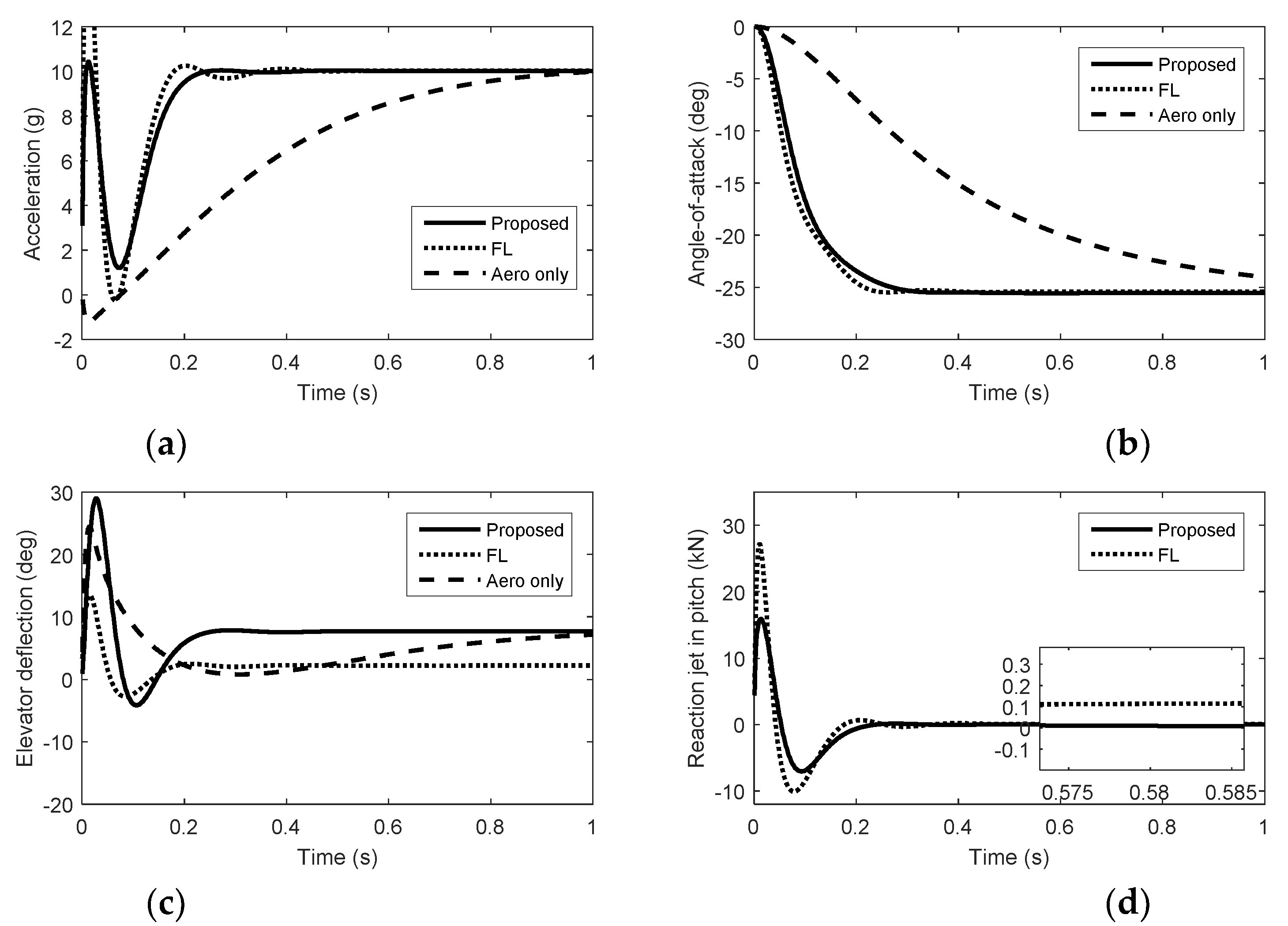
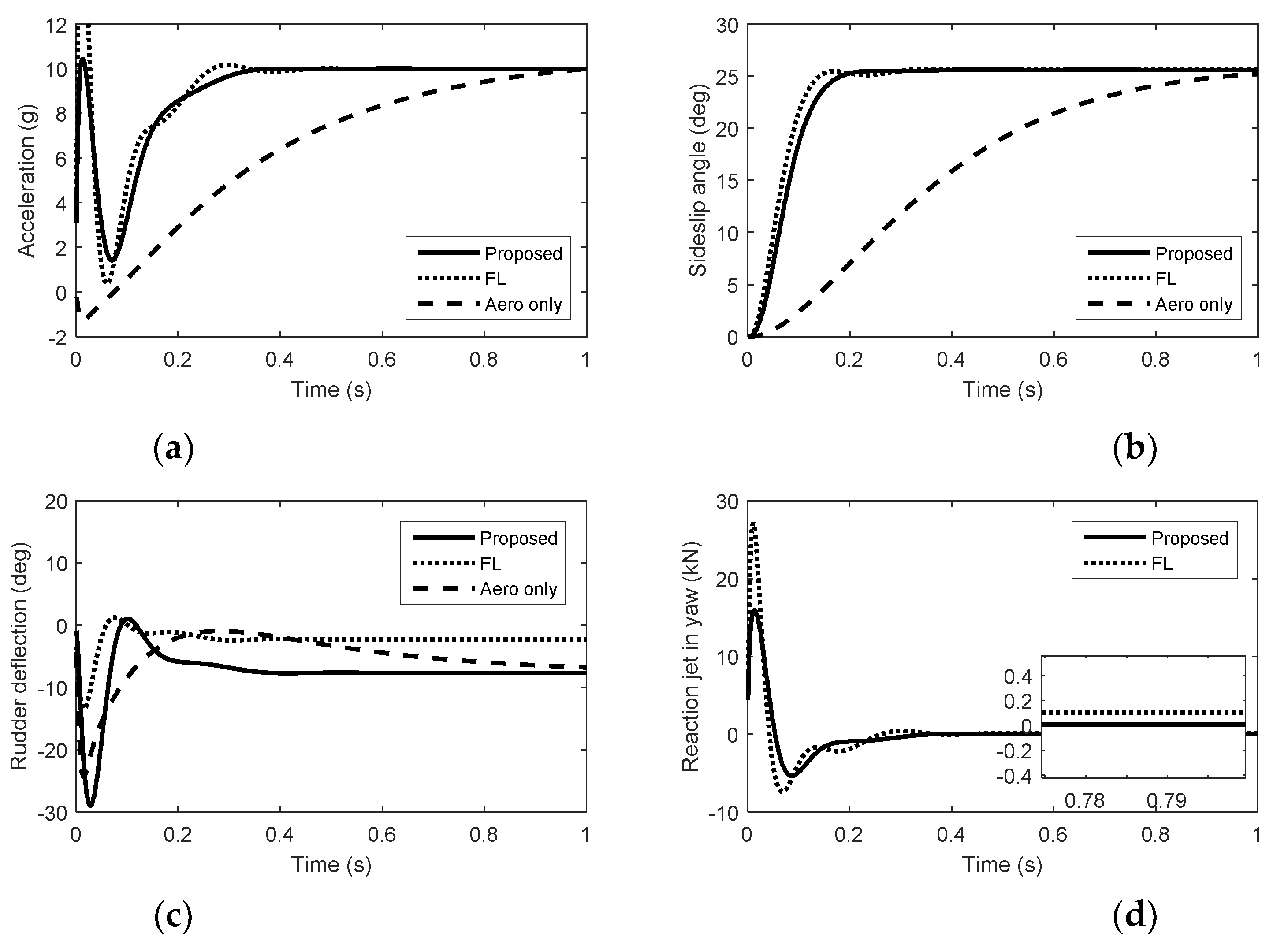
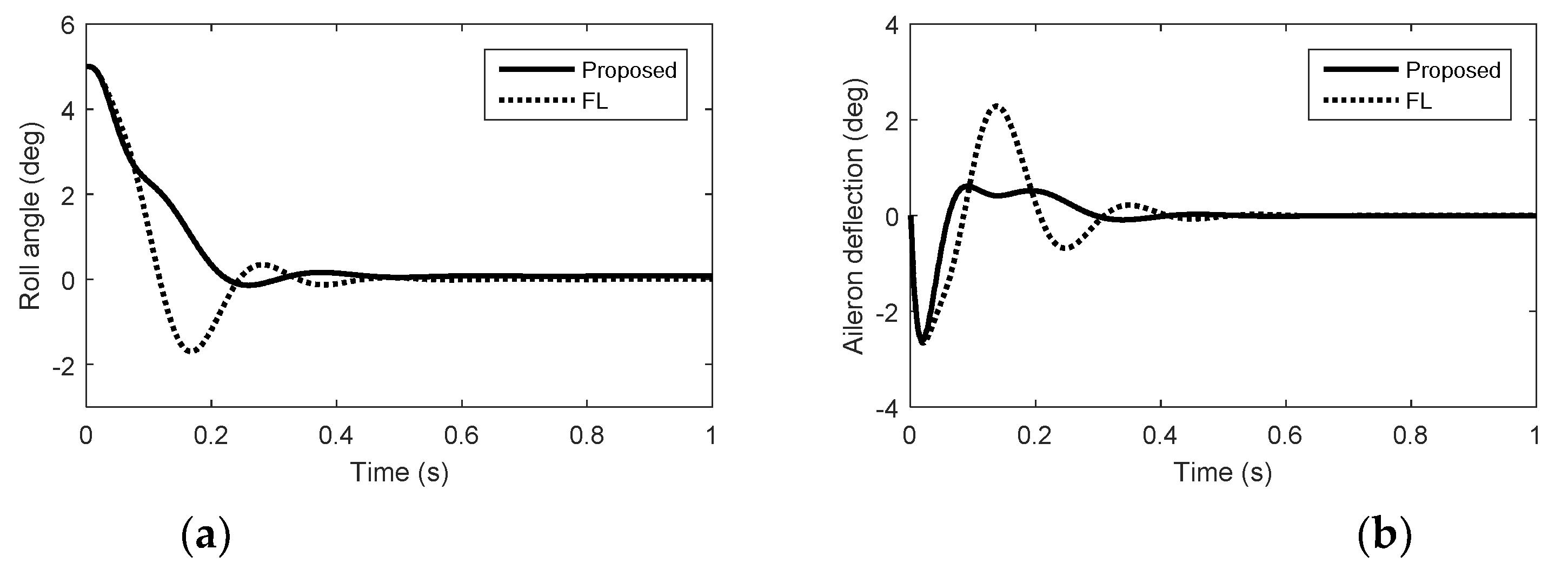
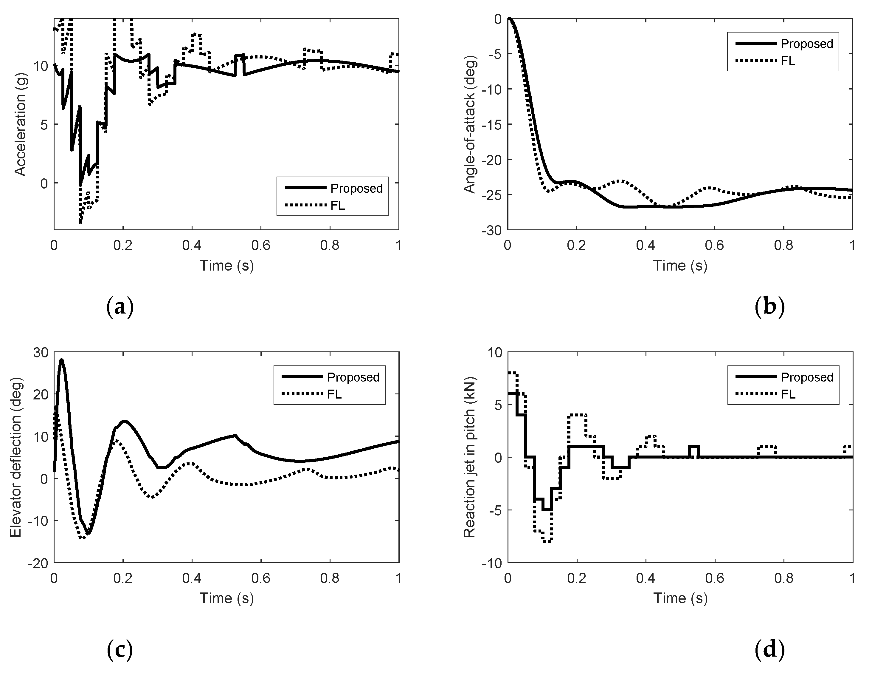
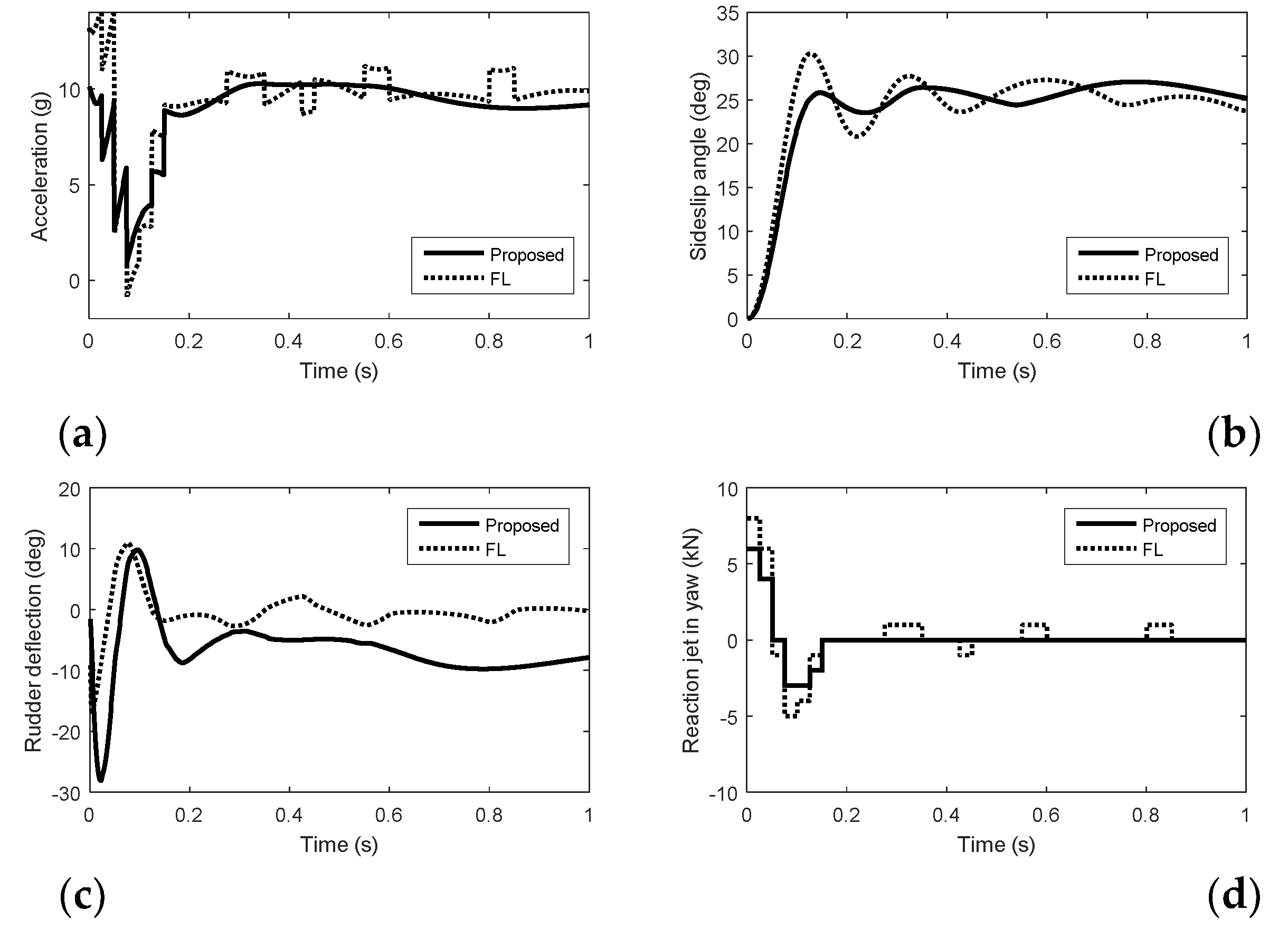
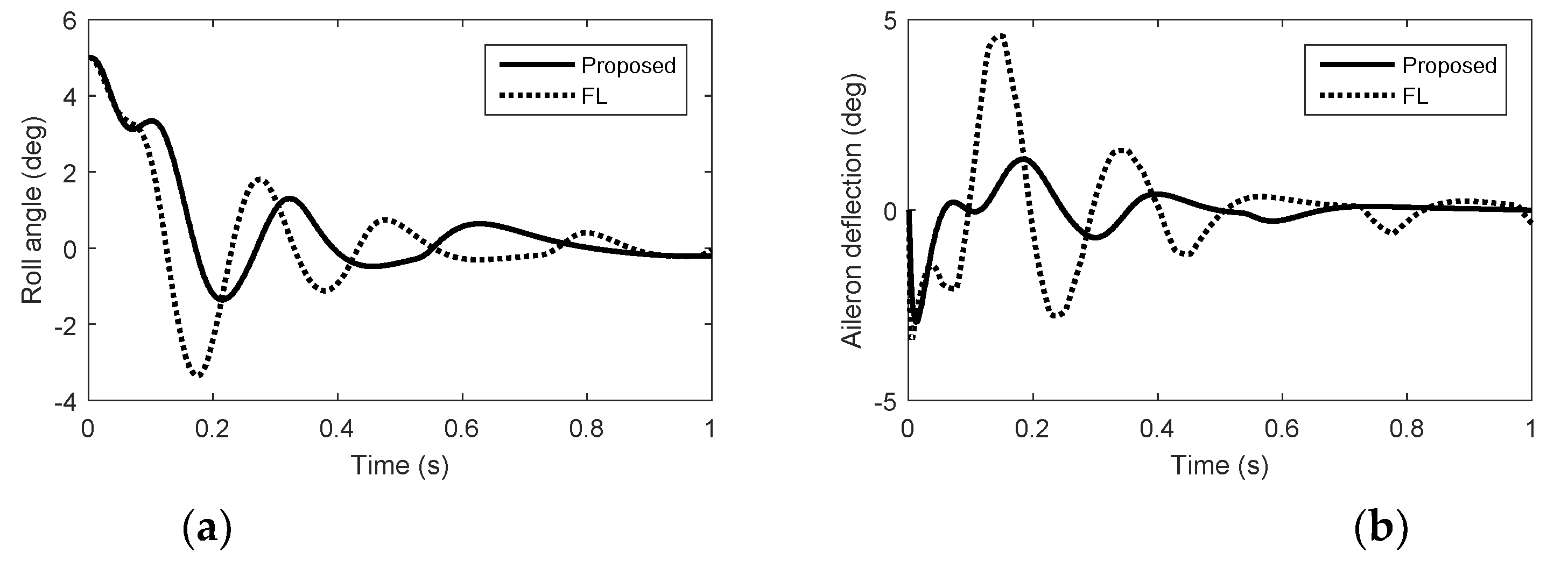
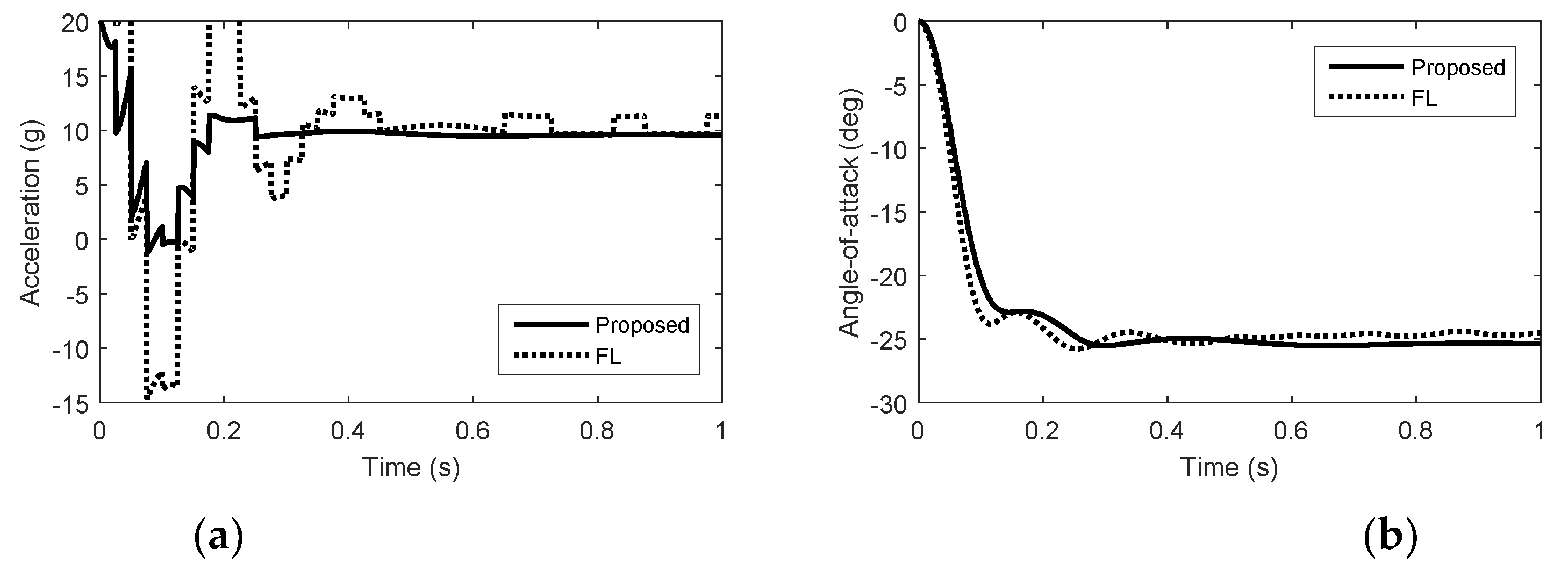
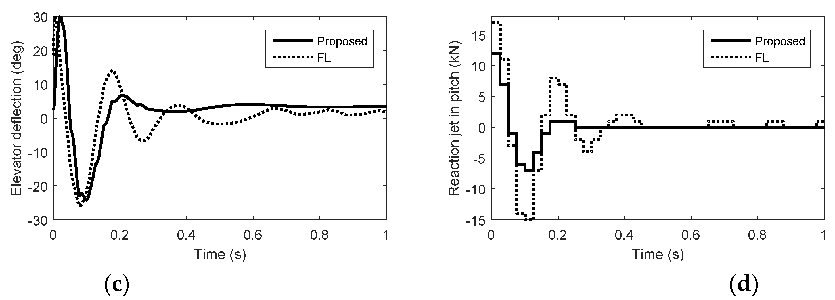
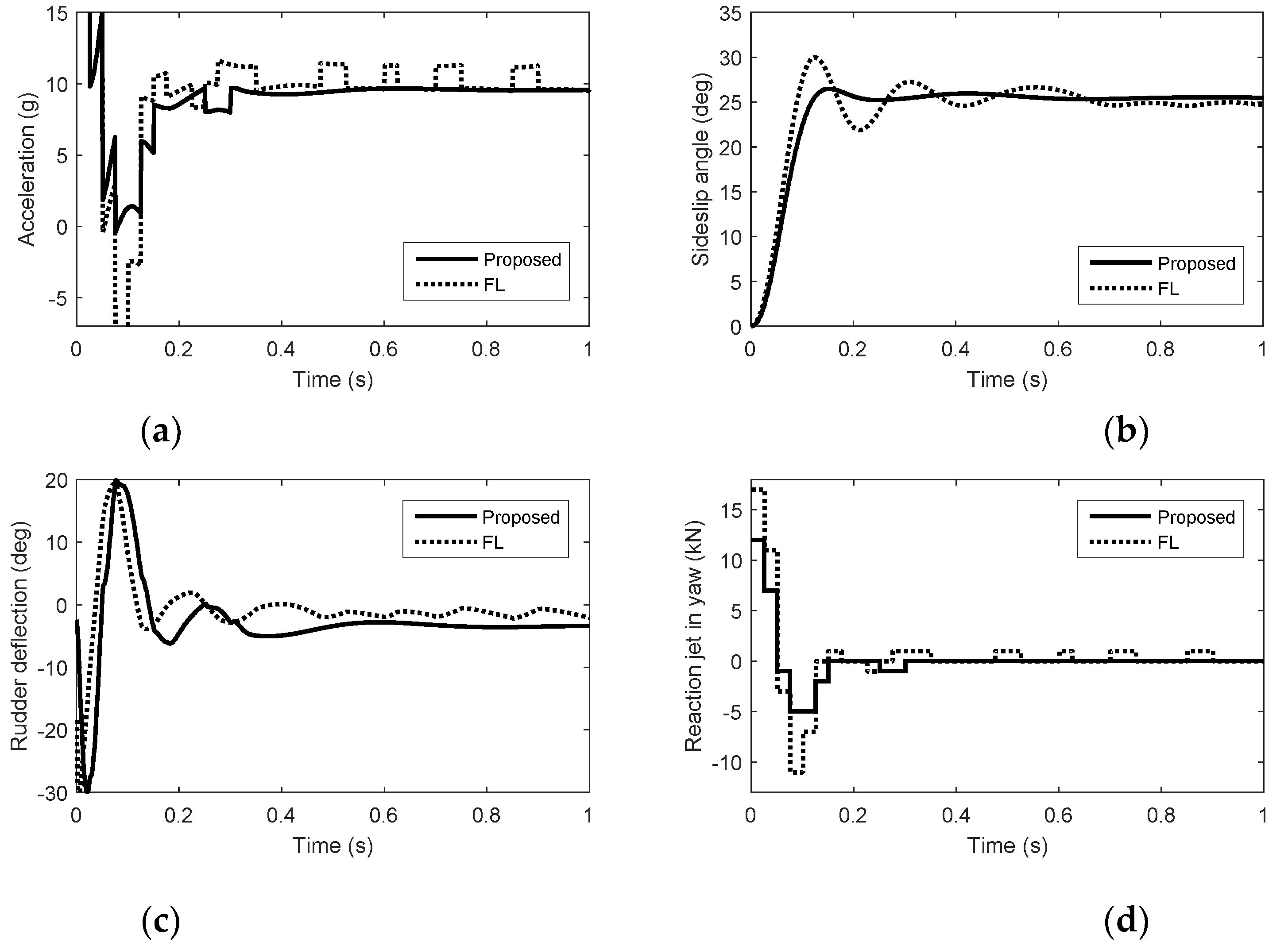
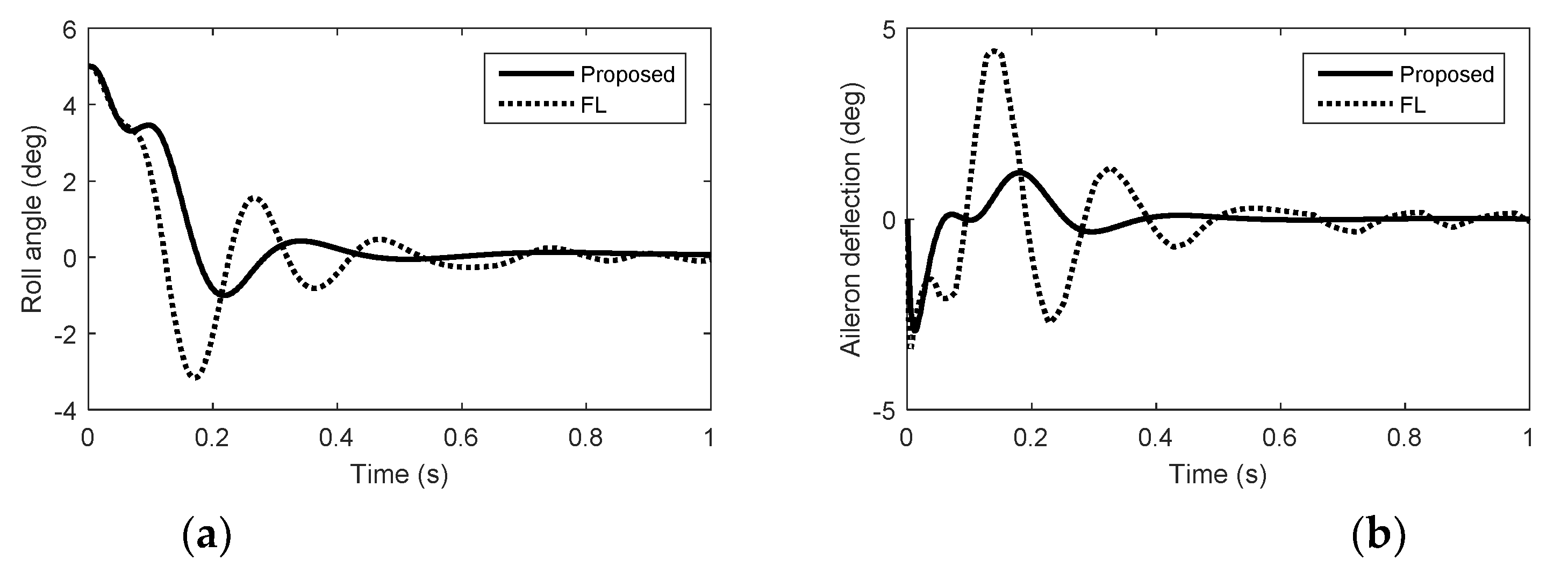
5. Simulation Results

In this section, the performance of the proposed fault tolerant control law for the interceptor is investigated by numerical simulations. The tracking acceleration commands are set to be N y = 10 g and N z = 10 g ; One pulse thrust can produce a force of 2500 N. The aerodynamic coefficients are obtained from [16]. The parameters of the virtual control law are chosen as k 1 = 10 , k 2 = 15 and k 3 = 20 ; The parameters of command filter are chosen as ω n = 10 r a d / s and ζ = 0.8 ; The matrices W 1 , W 2 and W 3 are chosen as W 1 = diag ( 3 , 3 , 1 , 3 , 1 ) , W 2 = diag ( 15 , 15 , 1 , 15 , 1 ) and W 3 = diag ( 5 , 5 , 1 , 5 , 1 ) . The parameters b k i and g τ i are b k i = 1 and g τ i = 1 . The desired control inputs δ y and δ z are chosen as δ y s = 0.015 N z c and δ z s = 0.015 N y c . In the simulation, the proposed fault tolerant control law is compared with the feedback linearization (FL) control law. The simulation results for the interceptor are shown in Figure 1, Figure 2 and Figure 3.
From Figure 1, Figure 2 and Figure 3, we can see that there is nonminimum phase phenomenon when the interceptor controlled purely by aerodynamic control surfaces. The acceleration response delay is large and the rise time under pure aerodynamic control is about 0.9 s. The introduction of the reaction system effectively compensates for this delay, significantly improving the speed of maneuver tracking. The interceptor with aerodynamic surfaces and reaction jets, under the proposed method and FL approach, there are no minimum phase phenomenon. The norm accelerations under the proposed method and FL are both stabilized after 0.2 s. However, the elevator and rudder deflections under FL are smaller than that under the proposed method and the forces generated by reaction jets under FL are larger than that under the proposed method, because under FL, the reaction jets and tail fins counteract each other after the angle-of-attack and sideslip angle have been generated. Therefore, it is hard to reach the fullest potential of aerodynamic control surfaces by the blending principle of FL. For the agile interceptor with two different types of actuators, the acceleration commands can be tracked by several combinations of inputs of the actuators. In the proposed approach, reaction jets cooperate with aerodynamic control surfaces very well and the fast response of the acceleration command can also be realized with less energy of the reaction jets by regulating the control allocation parameters. When the angle-of-attack and sideslip angle have been generated, the deflections of elevator and rudder under the proposed method are close to the case of aero only. The forces of reaction jets and aerodynamic control surfaces counteract each other under FL, which means the energy of the reaction jets is still consumed when the angle-of-attack and sideslip angle have been generated.
In practical applications, the reaction jets are pulsed control effectors modeled as zero-order holders with a sample time of 25 ms. Simulation results with quantization errors are given in Figure 4, Figure 5 and Figure 6.
The control system tracks the acceleration command smoothly under the proposed method than that under FL when the angle-of-attack and sideslip angle have been generated, because the norm acceleration is maintained by both aerodynamic control surfaces and reaction jets under FL. In Figure 1, Figure 2 and Figure 3, we can see that the forces of the reaction jets under FL in pitch and yaw do not converge to zero when the acceleration commands are tracked. In Figure 4, Figure 5 and Figure 6, when the angle-of-attack and sideslip angle are built up, the reaction jets under FL are still involved in controlling the attitude of the interceptor. The amount of pulse thrust consumption in pitch and yaw under the proposed method are 30 and 18, respectively, while the amount of pulse thrust consumption in pitch and yaw under FL are 57 and 33, respectively. Since the cooperation problem of the two different actuators are fully considered, the response speed of the proposed autopilot system is ensured while the consumption of pulse thrusts is reduced.
In the actuator fault case, we consider the damage of the aerodynamic control surfaces and the reaction control system failure due to the interactions between the airflow and the reaction jets. We suppose that the aerodynamic control surfaces lose 60% effectiveness and the reaction jets lose 50% effectiveness. Simulation results with quantization errors are given in Figure 7, Figure 8 and Figure 9. In Figure 7, Figure 8 and Figure 9, we can see that the autopilot system with FWDCA tracks norm acceleration commands fast and smoothly in the presence of the quantization errors and actuator faults. At 0.1 s, the acceleration under FL becomes negative, which is unexpected. The amount of pulse thrust consumption in pitch and yaw under the proposed method are 41 and 36, respectively, while the amount of pulse thrust consumption in pitch and yaw under FL are 106 and 61, respectively. Compared with no actuator faults, the amount of pulse thrust consumption increases by 60.4% under the proposed method, whereas the amount of pulse thrust consumption increases by 85.6% under the FL. In the case of actuator faults, the cooperation of the actuator of the proposed method is still better than FL.

6. Conclusions

In this paper, a fault tolerant control system with FWDCA is proposed for the interceptor with aerodynamic control surfaces and reaction jets in the presence of quantization errors and actuator faults. The nonlinear control system of the interceptor consists of a robust virtual control law and an FWDCA algorithm. The adaptive virtual control law is proposed by using command filtered backstepping with a parameter update law to produce virtual control signals. The hyperbolic tangent function is introduced to reduce the value of the nonlinear damping term. The FWDCA algorithm is proposed to optimally allocate the virtual signals to the actuators. In the proposed method, the cooperation problem of aerodynamic control surfaces and reaction jets is considered, the consumption of reaction jets is reduced. Simulation results show that the proposed control system tracks norm acceleration commands fast and smoothly under the quantization errors and actuator faults.

Author Contributions

Conceptualization, B.X. and J.Z.; methodology, B.X.; software, Q.M.; validation, B.X., Q.M. and J.F.; formal analysis, B.X.; investigation, B.X.; resources, Q.M.; data curation, Q.M.; writing—original draft preparation, B.X.; writing—review and editing, Q.M. and J.Z.; visualization, J.F.; supervision, B.X.; project administration, B.X.; funding acquisition, B.X. All authors have read and agreed to the published version of the manuscript.

Funding

This research was funded by National Natural Science Foundation of China grant number 61603183, Open Project Funds for the Key Laboratory of Space Photoelectric Detection and Perception, Ministry of Industry and Information Technology grant number NJ2022025-06, and Fundamental Research Funds for the Central Universities grant number NJ2022025.

Data Availability Statement

Data sharing is not applied.

Conflicts of Interest

The authors declare no conflict of interest.

References

  1. Zhou, D.; Xu, B. Adaptive dynamic surface guidance law with input saturation constraint and autopilot dynamics. J. Guid. Control Dyn. 2016, 39, 1152–1159. [Google Scholar] [CrossRef]
  2. Xu, B.; Zhou, D.; Liang, Z.; Zhou, G. Robust adaptive sliding sector control and control allocation of a missile with aerodynamic control surfaces and reaction jets. Proc. Inst. Mech. Eng. Part G: J. Aerosp. Eng. 2017, 231, 397–406. [Google Scholar] [CrossRef]
  3. Puchalski, R.; Giernacki, W. UAV fault detection methods, state-of-the-art. Drones 2022, 6, 330. [Google Scholar] [CrossRef]
  4. Dong, Z.; Liu, K.; Wang, S. Sliding mode disturbance observer-based adaptive dynamic inversion fault-tolerant control for fixed-wing UAV. Drones 2022, 6, 295. [Google Scholar] [CrossRef]
  5. Härkegard, O.; Glad, S.T. Resolving actuator redundancy—Optimal control vs. control allocation. Automatica 2005, 41, 137–144. [Google Scholar] [CrossRef]
  6. Thukral, A.; Innocenti, M. Sliding mode missile pitch autopilot synthesis for high angle of attack maneuvering. IEEE Trans. Control Syst. Technol. 1998, 6, 359–371. [Google Scholar] [CrossRef]
  7. Han, T.; Hu, Q. Robust autopilot design for STT missiles with multiple disturbances using twisting control. Aerosp. Sci. Technol. 2017, 70, 428–434. [Google Scholar] [CrossRef]
  8. Mohammadi, M.R.; Jegarkandi, M.F.; Moarrefianpour, A. Robust roll autopilot design to reduce couplings of a tactical missile. Aerosp. Sci. Technol. 2016, 51, 142–150. [Google Scholar] [CrossRef]
  9. Mattei, G.; Monaco, S. Nonlinear autopilot design for an asymmetric missile using robust backstepping control. J. Guid. Control Dyn. 2015, 37, 1462–1476. [Google Scholar] [CrossRef]
  10. Xin, M.; Balakrishnan, S.N. A new method for suboptimal control of a class of non-linear systems. Optim. Control Appl. Methods 2005, 26, 55–83. [Google Scholar] [CrossRef]
  11. Li, Q.; Zhou, D. Nonlinear autopilot design for interceptors with tail fins and pulse thrusters via θ-D approach. J. Syst. Eng. Electron. 2014, 25, 273–280. [Google Scholar] [CrossRef]
  12. Xin, M.; Balakrishnan, S.N. Nonlinear H∞ missile longitudinal autopilot design with θ-D method. IEEE Trans. Aerosp. Electron. Syst. 2008, 44, 41–56. [Google Scholar] [CrossRef]
  13. Choi, B.; Kang, S.; Kim, H.J.; Jun, B.E.; Lee, J.I.; Tahk, M.J.; Park, C. Roll-pitch-yaw integrated μ-synthesis for high angle-of-attack missiles. Aerosp. Sci. Technol. 2012, 23, 270–279. [Google Scholar] [CrossRef]
  14. Khalil, H. Nonlinear Systems, 3rd ed.; Prentice Hall: Englewood Cliffs, NJ, USA, 2002. [Google Scholar]
  15. Hu, Q.; Li, B.; Zhang, Y. Robust attitude control design for spacecraft under assigned velocity and control constraints. ISA Trans. 2013, 52, 480–493. [Google Scholar] [CrossRef]
  16. Zhou, D.; Shao, C. Dynamics and autopilot design for endoatmospheric interceptors with dual control systems. Aerosp. Sci. Technol. 2009, 13, 291–300. [Google Scholar] [CrossRef]
  17. Johansen, T.A.; Fossen, T.I. Control allocation—A survey. Autom. 2013, 49, 1087–1103. [Google Scholar] [CrossRef]
  18. Chang, Y.; Yuan, R.; Tan, X.; Yi, j. Observer-based adaptive sliding mode control and fuzzy allocation for aero and reaction jets’ missile. Proc. Inst. Mech. Eng. Part G: J. Aerosp. Eng. 2016, 230, 498–511. [Google Scholar] [CrossRef]
  19. Xing, L.; Zhang, K.; Chen, W. Optimal Control and Output Feedback Considerations for Missile with Blended Aero-fin and Lateral Impulsive Thrust. Chin. J. Aeronaut. 2010, 23, 401–408. [Google Scholar]
  20. Lei, R.; Chen, L. Adaptive fault-tolerant control based on boundary estimation for space robot under joint actuator faults and uncertain parameters. Def. Technol. 2019, 15, 964–971. [Google Scholar] [CrossRef]
  21. Alwi, H.; Edwards, C. Fault tolerant control using sliding modes with on-line control allocation. Autom. 2008, 44, 1859–1866. [Google Scholar] [CrossRef]
  22. He, J.; Qi, R.; Jiang, R.; Zhai, R. Fault-tolerant control with mixed aerodynamic surfaces and RCS jets for hypersonic reentry vehicles. Chin. J. Aeronaut. 2017, 30, 780–795. [Google Scholar] [CrossRef]
  23. Härkegard, O. Dynamic control allocation using constrained quadratic programming. J. Guid. Control Dyn. 2004, 27, 1028–1034. [Google Scholar] [CrossRef]
  24. Brierley, S.D. and Longchamp, R. Application of sliding-mode control to air-air interception problem. IEEE Trans. Aerosp. Electron. Syst. 1990, 26, 306–325. [Google Scholar] [CrossRef]
  25. Manchester, I.R.; Savkin, A.V. Circular navigation missile guidance with incomplete information and uncertain autopilot model. J. Guid. Control Dyn. 2004, 27, 1078–1083. [Google Scholar]
  26. Reisner, D. and Shima, T. Optimal guidance-to-collision law for an accelerating exoatmospheric interceptor missile. J. Guid. Control Dyn. 2013, 36, 1695–1708. [Google Scholar] [CrossRef]
  27. Dong, W.; Farrell, J.A.; Polycarpou, M.M.; Djapic, V.; Sharma, M. Command filtered adaptive backstepping. IEEE Trans. Cotrol Syst. Technol. 2012, 20, 566–580. [Google Scholar] [CrossRef]
Figure 1. Simulation results in pitch. (a) Acceleration. (b) Angle of attack. (c) Elevator deflection. (d) Reaction jet in pitch.
Drones 07 00106 g001
Figure 2. Simulation results in yaw. (a) Acceleration. (b) Sideslip angle. (c) Rudder deflection. (d) Reaction jet in yaw.
Drones 07 00106 g002
Figure 3. Simulation results in roll. (a) Roll angel. (b) Aileron deflection.
Drones 07 00106 g003
Figure 4. Simulation results in pitch with quantization errors. (a) Acceleration. (b) Angle of attack. (c) Elevator deflection. (d) Reaction jet in pitch.
Drones 07 00106 g004
Figure 5. Simulation results in yaw with quantization errors. (a) Acceleration. (b) Sideslip angle. (c) Rudder deflection. (d) Reaction jet in yaw.
Drones 07 00106 g005
Figure 6. Simulation results in roll with quantization errors. (a) Roll angel. (b) Aileron deflection.
Drones 07 00106 g006
Figure 7. Simulation results in pitch with quantization errors and actuator faults. (a) Acceleration. (b) Angle of attack. (c) Elevator deflection. (d) Reaction jet in pitch.
Drones 07 00106 g007aDrones 07 00106 g007b
Figure 8. Simulation results in yaw with quantization errors and actuator faults. (a) Acceleration. (b) Sideslip angle. (c) Rudder deflection. (d) Reaction jet in yaw.
Drones 07 00106 g008
Figure 9. Simulation results in yaw with quantization errors and actuator faults. (a) Roll angel. (b) Aileron deflection.
Drones 07 00106 g009
Disclaimer/Publisher’s Note: The statements, opinions and data contained in all publications are solely those of the individual author(s) and contributor(s) and not of MDPI and/or the editor(s). MDPI and/or the editor(s) disclaim responsibility for any injury to people or property resulting from any ideas, methods, instructions or products referred to in the content.

