Using Drones to Monitor Broad-Leaved Orchids (Dactylorhiza majalis) in High-Nature-Value Grassland

Abstract

Dactylorhiza majalis is a threatened indicator species for the habitat quality of nutrient-poor grassland sites. Environmentalists utilize the species to validate the success of conservation efforts. Conventionally, plant surveys are field campaigns where the plant numbers are estimated and their spatial distribution is either approximated by GPS or labor-intensively measured by differential GPS. In this study, we propose a monitoring approach using multispectral drone-based data with a very high spatial resolution (~3 cm). We developed the magenta vegetation index to enhance the spectral response of Dactylorhiza majalis in the drone data. We integrated the magenta vegetation index in a random forest classification routine among other vegetation indices and analyzed feature impact on model decision making using SHAP. We applied an image object-level median filter to the classification result to account for image artefacts. Finally, we aggregated the filtered result to individuals per square meter using an overlaying vector grid. The SHAP analysis showed that magenta vegetation index had the highest impact on model decision making. The random forest model could reliably classify Dactylorhiza majalis in the drone data (F1 score: 0.99). We validated the drone-derived plant count using field mappings and achieved good results with an RMSE of 12 individuals per square meter, which is within the error margin stated by experts for a conventional plant survey. In addition to abundance, we revealed the comprehensive spatial distribution of the plants. The results indicate that drone surveys are a suitable alternative to conventional monitoring because they can aid in evaluating conservation efforts and optimizing site-specific management.

1. Introduction

Dactylorhiza majalis (DM) or broad-leaved marsh orchid is an indicator species for the habitat quality of nutrient-poor grassland sites. The species is widespread across Europe, and a significant portion of the population grows in Germany [1,2]. However, DM used to be far more common in Germany’s grasslands in the 1950s. Conservationists have reported a strong decline in the national population for at least the past 20 years [1,3,4]. Due to the severe decline, the federal agency of nature conservation and all state agencies of nature conservation in Germany list DM on the Red List of species threatened with extinction [2]. Furthermore, central European countries have reported a similar decline in DM population, e.g., the Czech Republic [5] or Switzerland [6]. Likewise, they list the species in their national or regional lists of species threatened with extinction.

The causes of decline are generally agreed upon; intensification of agriculture, water drainage, scrub encroachment due to habitat abandonment, and forestation negatively impact the habitat conditions [1,2,3,4,5]. Conservationists have tried counteracting the population decline by restoring the species’ original habitat conditions, but the success of the conservation measures remains to be seen. To support the conservation measures, regular monitoring of the population development is required. Conventional mapping approaches assess the population size in labor-intensive field campaigns where plants are counted manually [3] or the population size is estimated by extrapolation from small samples [4]. These approaches, however, become infeasible and increasingly error-prone with increasing size and inaccessibility of the study site. The aforementioned problems may additionally limit the surveyor’s ability to accurately describe the spatial distribution of orchids during monitoring, which is valuable insight into whether conservation measures are successful.

Remote sensing techniques, however, can cope with these scaling problems [7]. Moreover, previous studies reported promising results in detecting spectrally distinguishable flowers using remote sensing techniques. For example, the authors of [8] applied a threshold image segmentation on multispectral imagery to detect peach blossoms. The authors of [9] developed a support vector machine classification-based approach to estimate vegetation fraction and flower fraction in oilseed rape from multispectral imagery. The authors of [10] demonstrated how to combine hyperspectral data and a random forest classification to gain knowledge on the flower cycle and spatial abundance of flowering plants in the context of a bee health study. During flowering between the beginning of May and mid-July, DM also builds an inflorescence with magenta-colored flowers. This spectrally prominent feature may be a basis for remote-sensing-based monitoring.

Some studies used satellite [11,12] or airborne data [10,13] to identify flowers; the majority, however, utilized drone imagery [8,9,14,15,16,17], since drones can provide data with a very high spatial resolution. This kind of data allows identifying small vegetation structures such as flowers or flower heads [14]. There is, however, a lack of vegetation indices to detect magenta-colored flowers. To identify DM, we focused on the unique spectral response of the flower color which interferes with the concept of conventional vegetation indices. Multiple studies observed decreased values of indices such as the normalized difference vegetation index (NDVI) or the enhanced vegetation index (EVI) when colored flowers were prominently present in remote sensing data [12,18,19,20]. The flower colors increase the reflectance in the red wavelengths, which in return decreases the value of all near-infrared (NIR)/red ratio-based vegetation indices. Over the last decade, multiple studies incorporated this characteristic to detect flowers [8,9]; moreover, some studies designed new indices to detect specific flower colors [12,21]. We, therefore, propose a new vegetation index called the magenta vegetation index (MaVI) that enhances the spectral characteristics of magenta-colored flowers. However, a magenta flower color is not a unique characteristic among flowering plants. Although the index was developed for DM, it is reasonable to assume that the MaVI can also be used for species with similar flower color, e.g., Lythrum salicaria or Dactylorhiza incarnata. On the one hand, this implies a certain flexibility and multiple uses of the MaVI. On the other hand, a potential cooccurrence of flowers with similar color may lead to ambiguous results. For this study, however, local conservationists confirmed that DM was the only magenta-colored plant species in the study site during the drone flight.

Given the need to regularly monitor DM while the resources for nature conservation are limited and the lack of a specialized remote sensing toolbox, we present a drone-based monitoring approach that aims to fill this gap. With this approach, we aim to estimate the population size and assess the spatial abundance of DM using multispectral, very-high-spatial-resolution drone data (3.4 cm pixel size). We acquired the data during the flowering phase of DM to map individual inflorescences. In this paper, we provide the methodological framework and evaluate our approach in comparison to conventional in-situ monitoring. The specific objectives of this case study were to (1) determine highly predictive features to identify DM, (2) evaluate the predictive performance of the MaVI, (3) quantify the accuracy of a drone-based plant count in comparison to conventional DM monitoring, and (4) demonstrate a practical way to bridge the gap between remote sensing and ecological applications.

2. Materials and Methods

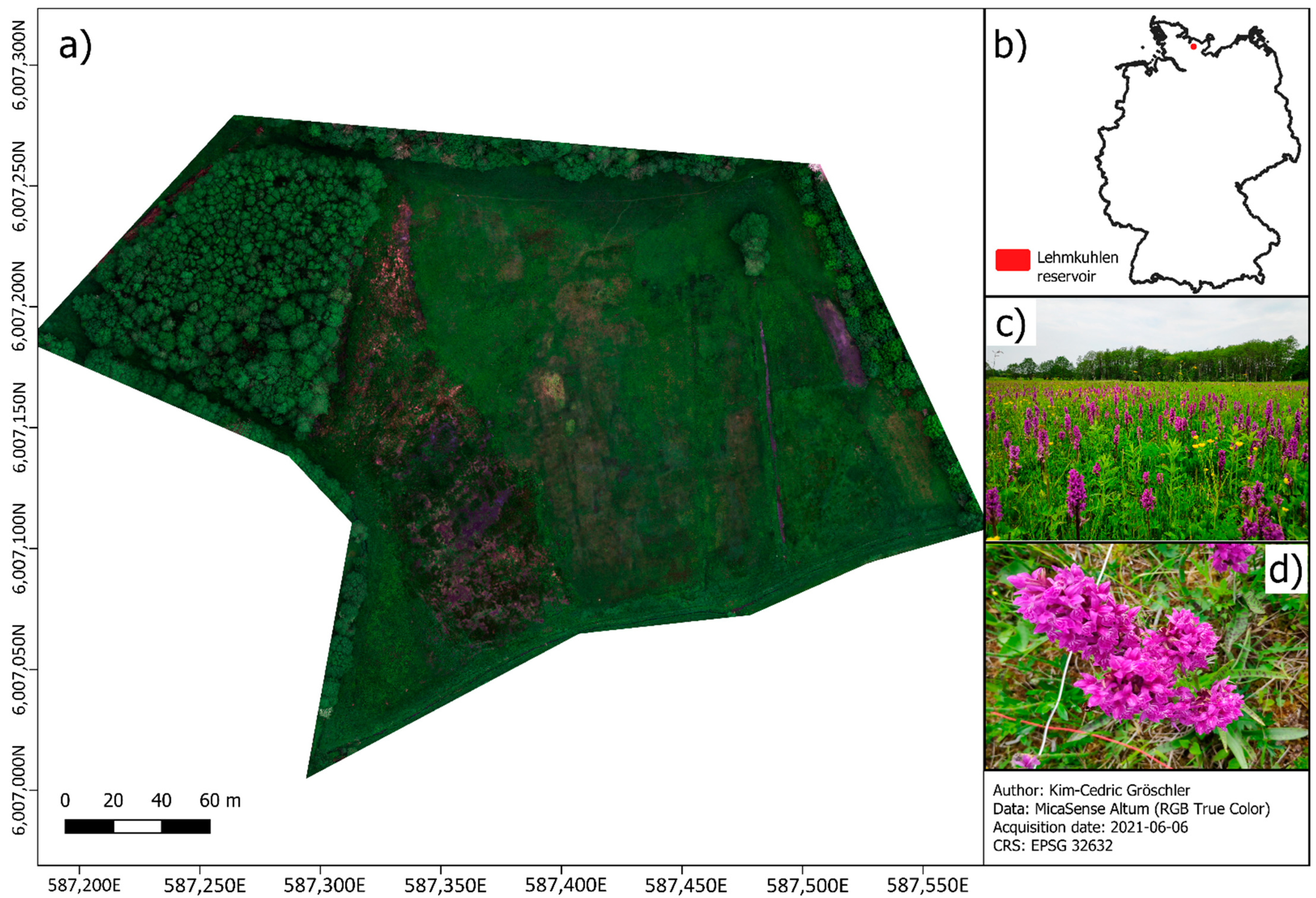
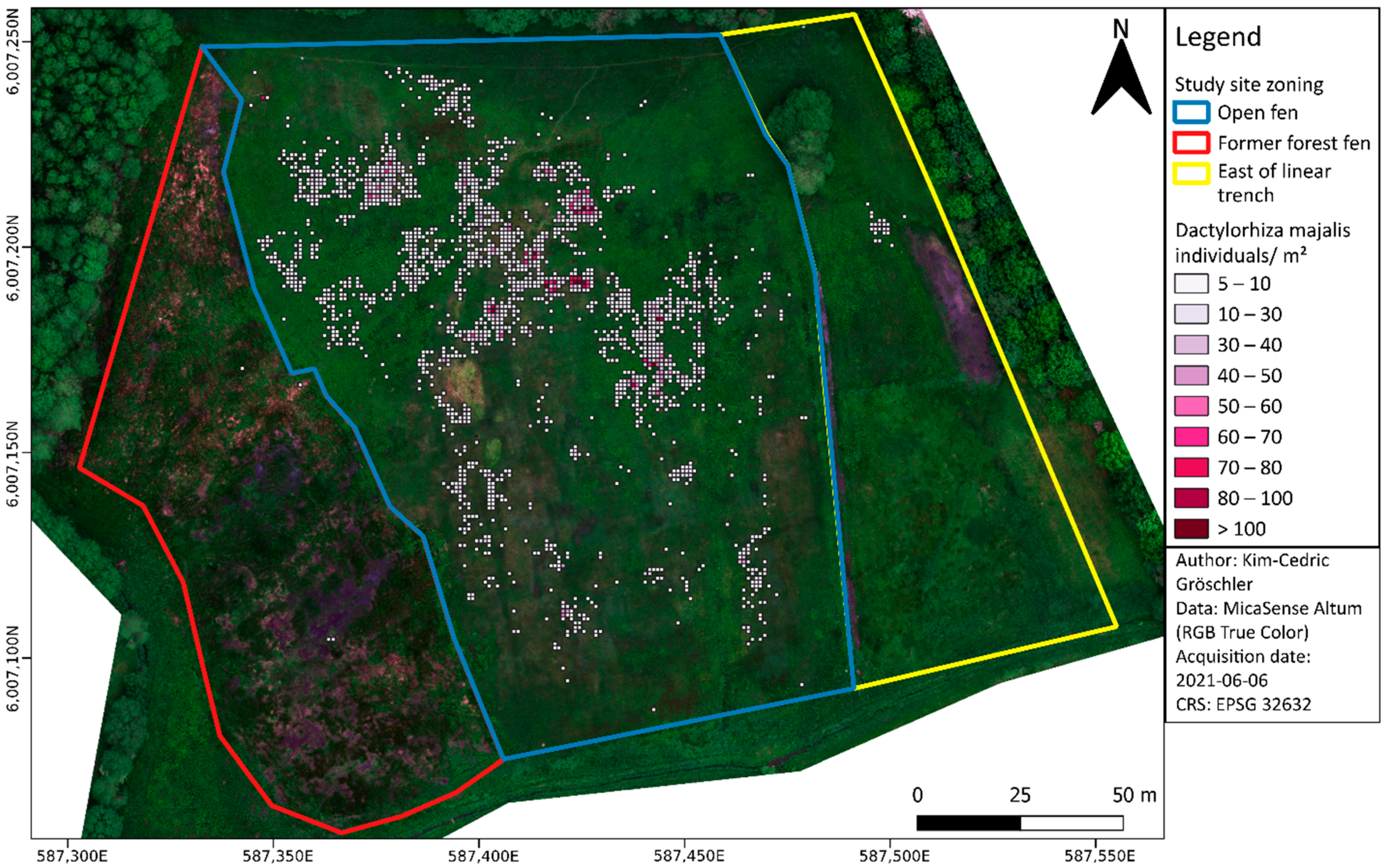
2.1. Study Site

We conducted this study in the Lehmkuhlen reservoir (Figure 1), an alkaline, nutrient-poor fen in the uplands of Schleswig-Holstein, Germany, which reported the biggest state-wide DM population [22]. As a part of the uplands of Schleswig-Holstein, the Lehmkuhlen reservoir was formed during the Weichselian ice age [23]. At that time, the area originated as a lake but transitioned into a fen over time. Since the 1950s, parts of the Lehmkuhlen reservoir transformed into a forest fen. With an area of 0.29 km², it is a small but species-rich area, where 60 plant species threatened with extinction including DM are reported [22,23]. The Lehmkuhlen reservoir, therefore, is protected by the European habitat directive due to the occurrence of alkaline fens (Nature 2000 code: FFH 7230) and transition mires (Nature 2000 code: FFH 7140) [24]. Due to the ecological importance of the area, conservation measures are conducted to preserve the rare habitat conditions [24]. In 2011, parts of the forest were removed to increase the development potential of endangered plant species. To prevent scrub encroachment in the open fen and retain favorable conditions for competitively weak plant species, conservationists mow the area once a year.

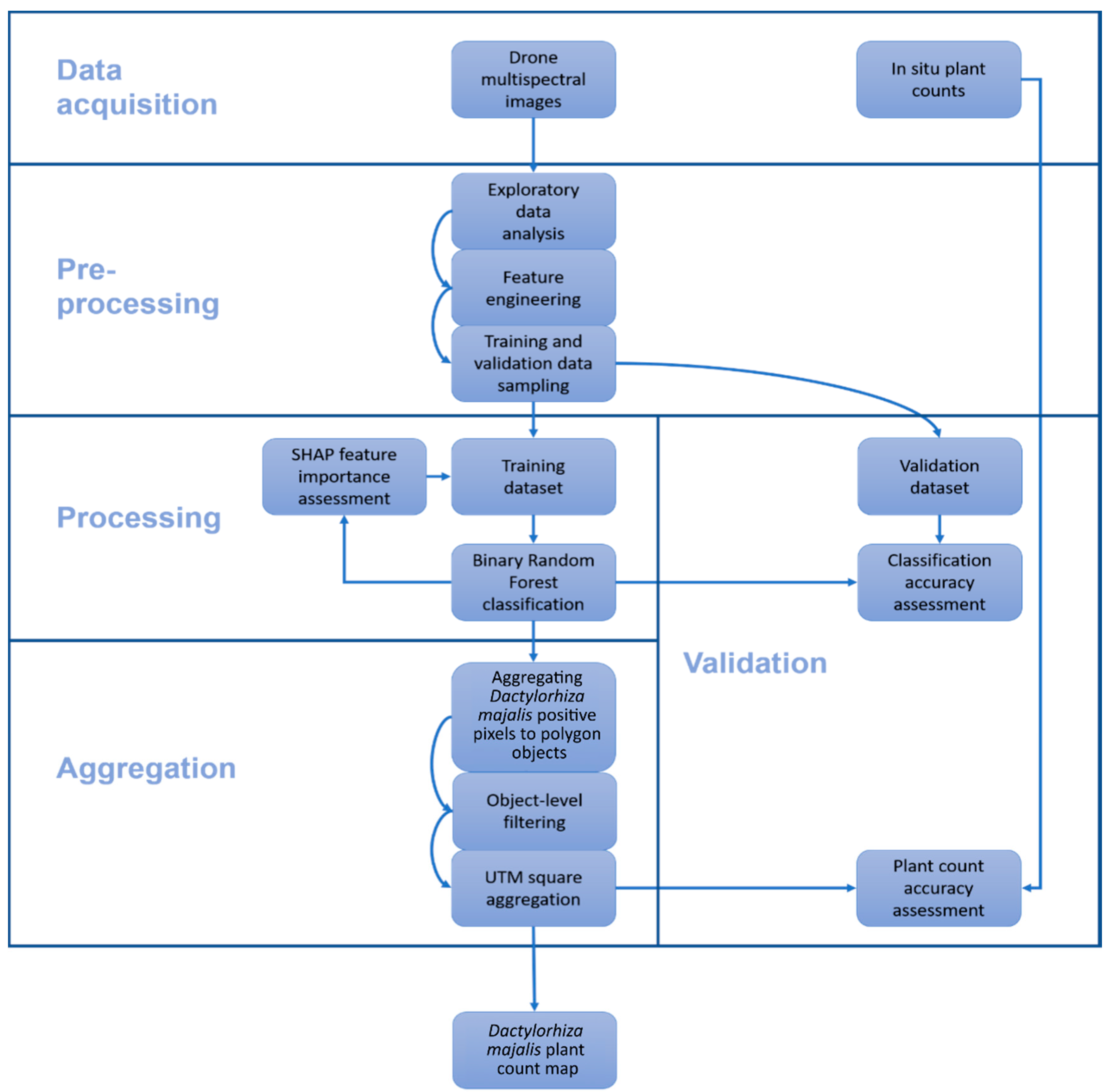
2.2. Data (Pre-)Processing and Analysis

Figure 2 illustrates the methodological workflow of this study, which is divided into data acquisition, preprocessing, processing, aggregation, and validation. Data acquisition includes drone flight and field mapping. The preprocessing covers exploratory data analysis, subsequent feature engineering, and the creation of a reference dataset for model training and validation. During processing, we trained a random forest classifier and evaluated feature importance and interactions; we further removed redundant or nonpredictive features from the training dataset, retrained the model with the best-performing set of features, and applied the retrained classifier to the drone dataset before we assessed the accuracy of the classification results. In the following aggregation, we polygonized classified pixel clusters (i.e., pixels of the same class in direct proximity) to vector image objects and applied an object-level filtering approach to remove invalid pixels from the subsequent inflorescence count. We assessed the accuracy of the remote-sensing-derived plant count by comparison with our field mapping results. In a final step, the resulting inflorescences were summed up to individuals per square meter in a Universal Transverse Mercator coordinate system.

2.3. Drone Data

Aerial images were taken during the flowering phase of DM on 6 July 2021, using a Wingtra One drone [25]. The weather during the flight was calm and consistently overcast. The overcast weather ensured a stable source of illumination during flight, thereby limiting the spectral variability between different images. The drone was equipped with a MicaSense Altum multispectral camera with spectral bands in the blue, green, red, red-edge, and near-infrared regions(refer to [26] for band designation). The camera had a focal length of 8 mm and a field of view of 48° × 37°. Each band captured data with 3.2 megapixels resulting in an image size of 2046 × 1544 pixels. The mean flight altitude was 150 m. Flight planning and configuration were conducted using the proprietary mission control software WingtraPilot. The raw image data were processed to surface reflectance with the Pix4D mapper software version 4.6.4 by the commissioned company. In total, 3695 images were processed to a single orthomosaic with a spatial resolution of 3.4 cm.

2.4. In Situ Data

On the day of the drone flight, we conducted in situ measurements to collect validation data for the remote sensing plant count. The in situ plant counts followed an established methodology in ecology [1,27], i.e., we used a 1 m² frame, placed it randomly in the study site, and counted all plants of the target species within the square twice. We then took a top-down photo for reference and defined the center location of the square using a Global Positioning System (GPS) device (Garmin fēnix 5). In total, we performed 10 in situ plant counts at the study site. Additionally, we measured the inflorescence diameter of some randomly selected plants to approximate the average spatial coverage of a DM inflorescence. This measure was used for comparison with the spatial resolution of the drone data. The measurements showed that the average inflorescence diameter of DM was approximately equal to or slightly smaller than the spatial resolution of the drone dataset.

2.5. Labeling a Reference Dataset for Model Training and Validation

To identify DM, we created a reference dataset containing a DM-positive and a DM-negative class by applying a split sampling strategy. For the DM-positive class, we selected 2000 pixels on the basis of a visual inspection of the drone data. For the DM-negative class, we applied a pseudo-random sampling approach recommended by [28]. We undersampled the DM negative class since it made up the majority of the pixels. We used the QGIS “random points in extent” function to randomly select 2000 points in the study site and subsequently sample the underlying pixel values. We manually labeled these pixels by visual interpretation and removed all DM-positive pixels. The missing pixels were iteratively replaced by new randomly selected pixels until all pixels belonged to the DM-negative class. In summary, the reference dataset was balanced and consisted of 4000 pixels (2000 pixels for each class). Subsequently, we split the reference dataset into a training and holdout dataset for model training and independent evaluation (refer to Section 2.7).

Within the scope of image classification, a pixel can hold different values, i.e., features. In this study, the list of features included the spectral reflectances of the available drone bands and a series of vegetation indices we calculated for the subsequent analysis (see

Table 1. Vegetation indices considered for this study’s random forest classification. Abbreviations: B = blue band; G = green band; R = red band; NIR = near-infrared band.

Vegetation Index	Formula	Reference
Atmospherically resistant vegetation index (ARVI)	$\mathrm{ARVI}=\frac{\mathrm{NIR}-\mathrm{R}-\mathrm{y}\left(\mathrm{R}-\mathrm{B}\right)}{\mathrm{NIR}+\mathrm{R}-\mathrm{y}\left(\mathrm{R}-\mathrm{B}\right)}$ y = 1	[29]
Adjusted transformed soil-adjusted vegetation index (ATSAVI)	$\mathrm{ATSAVI}=\mathrm{a}\frac{\mathrm{NIR}-\mathrm{a}\times \mathrm{R}-\mathrm{b}}{\mathrm{a}\times \mathrm{NIR}+\mathrm{R}-\mathrm{a}\times \mathrm{b}+\mathrm{X}\left(1+{\mathrm{a}}^2\right)}$ a = 1.22, X = 0.08, b = 0.03	[30]
Blue-wide dynamic range vegetation index (BWDRVI)	$\mathrm{BWDRVI}=\frac{0.1\mathrm{NIR}-\mathrm{B}}{0.1\mathrm{NIR}+\mathrm{B}}$	[31]
Chlorophyll vegetation index (CVI)	$\mathrm{CVI}=\mathrm{NIR}\frac{\mathrm{R}}{{\mathrm{G}}^2}$	[32]
Enhanced bloom index (EBI)	$\mathrm{EBI}=\frac{\mathrm{R}+\mathrm{G}+\mathrm{B}}{\frac{\mathrm{G}}{\mathrm{B}}\times \left(\mathrm{R}-\mathrm{B}+\mathsf{\epsilon }\right)}$ ε = 1	[22]
Enhanced vegetation index (EVI)	$\mathrm{EVI}=2.5\frac{\mathrm{NIR}-\mathrm{R}}{\left(\mathrm{NIR}+6\mathrm{R}-7.5\mathrm{B}\right)+1}$	[33]
Green atmospherically resistant vegetation index (GARI)	$\mathrm{GARI}=\frac{\mathrm{NIR}-\left(\mathrm{G}-\left(\mathrm{B}-\mathrm{R}\right)\right)}{\mathrm{NIR}-\left(\mathrm{G}+\left(\mathrm{B}-\mathrm{R}\right)\right)}$	[34]
Green leaf index (GLI)	$\mathrm{GLI}=\frac{2\mathrm{G}-\mathrm{R}-\mathrm{B}}{2\mathrm{G}+\mathrm{R}+\mathrm{B}}$	[35]
Green–blue normalized difference vegetation index (GBNDVI)	$\mathrm{GBNDVI}=\frac{\mathrm{NIR}-\left(\mathrm{G}+\mathrm{B}\right)}{\mathrm{NIR}+\left(\mathrm{G}+\mathrm{B}\right)}$	[36]
Green–red normalized difference vegetation index (GRNDVI)	$\mathrm{GRNDVI}=\frac{\mathrm{NIR}-\left(\mathrm{G}+\mathrm{R}\right)}{\mathrm{NIR}+\left(\mathrm{G}+\mathrm{R}\right)}$	[36]
Green–red vegetation index (GRVI)	$\mathrm{GRVI}=\frac{\mathrm{G}-\mathrm{R}}{\mathrm{G}+\mathrm{R}}$	[37]
Normalized difference vegetation index (NDVI)	$\mathrm{NDVI}=\frac{\mathrm{NIR}-\mathrm{R}}{\mathrm{NIR}+\mathrm{R}}$	[38]
Renormalized difference vegetation index (RDVI)	$\mathrm{RDVI}=\frac{\mathrm{NIR}-\mathrm{R}}{{\left(\mathrm{NIR}+\mathrm{R}\right)}^{0.5}}$	[39]
Soil and atmospherically resistant vegetation index (SARVI)	$\mathrm{SARVI}=\left(1+\mathrm{L}\right)\frac{\mathrm{NIR}-\left(\mathrm{R}-\mathrm{y}\times \left(\mathrm{B}-\mathrm{R}\right)\right)}{\mathrm{NIR}+\left(\mathrm{R}-\mathrm{y}\times \left(\mathrm{B}-\mathrm{R}\right)\right)+\mathrm{L}}$ L = 0.5 y = 1	[30]
Adjusted transformed soil-adjusted vegetation index (SAVI)	$\mathrm{SAVI}=\frac{\mathrm{NIR}-\mathrm{R}}{\mathrm{NIR}+\mathrm{R}+\mathrm{L}}\times \left(1+\mathrm{L}\right)$ L = 0.5	[30]
Transformed soil-adjusted vegetation index (TSAVI)	$\mathrm{TSAVI}=\frac{\mathrm{s}\left(\mathrm{NIR}-\mathrm{s}\times \mathrm{R}-\mathrm{a}\right)}{\mathrm{a}\times \mathrm{NIR}+\mathrm{R}-\mathrm{a}\times \mathrm{s}+\mathrm{X}\times \left(1+\mathrm{s}²\right)}$ s = 0.33 a = 0.5 X = 1.5	[30]
Wide dynamic range vegetation index (WDRVI)	$\mathrm{WDRVI}=\frac{0.1\mathrm{NIR}-\mathrm{R}}{0.1\mathrm{NIR}+\mathrm{R}}$	[40]

). All vegetation indices incorporated in the subsequent random forest classification routine except for the MaVI are listed in Table 1. We describe the ideas and implementation of the MaVI in detail in the next section.

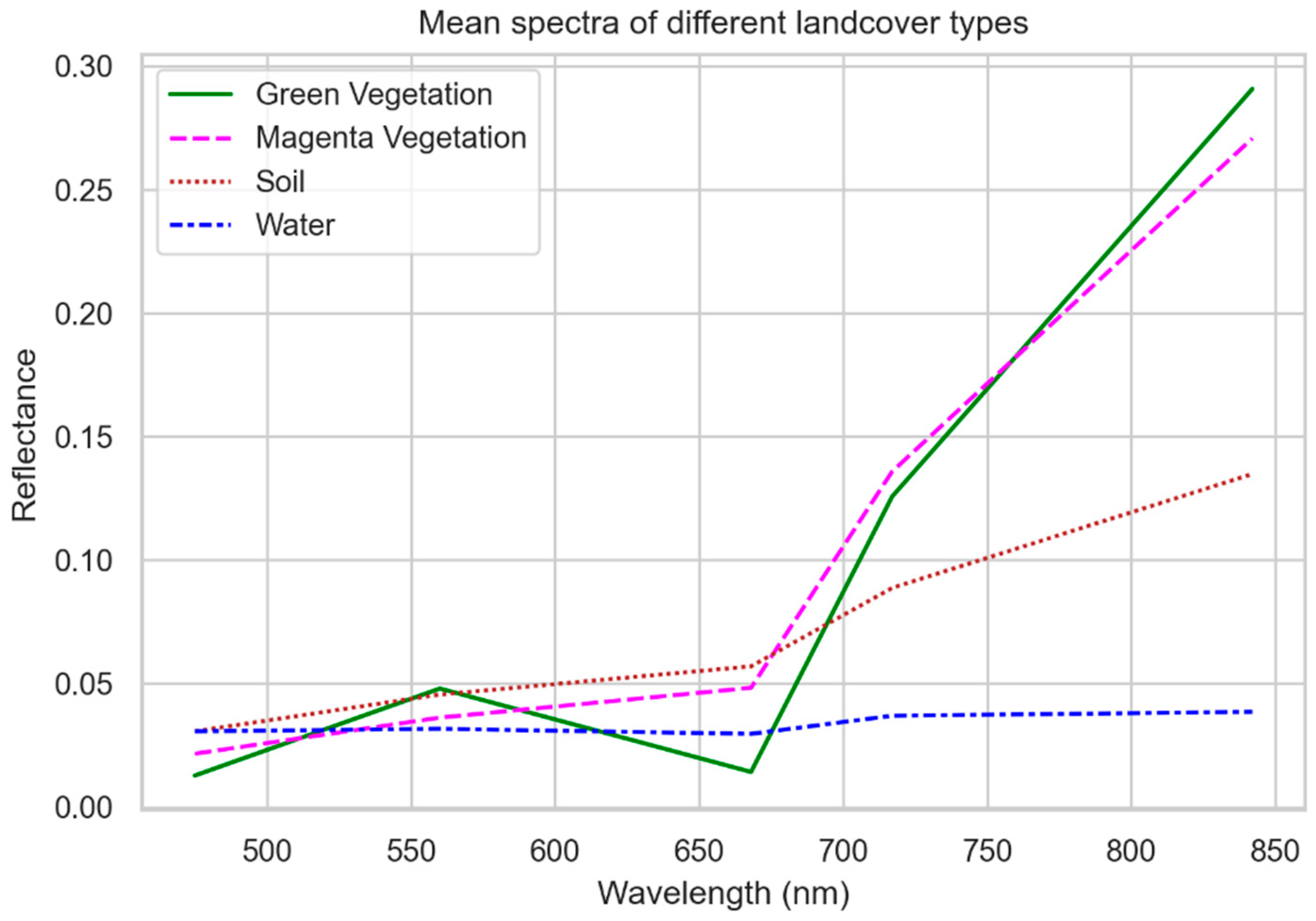
2.6. Magenta Vegetation Index—Main Ideas and Practical Implementation

We analyzed the spectral signatures of different land-cover types in the Lehmkuhlen reservoir to identify spectral characteristics of magenta-colored vegetation (Figure 3). We found that magenta-colored flowers tended to have relatively high reflectance values in the blue and red bands, while green vegetation showed the characteristic green peak. We identified the highest potential to differentiate magenta-colored vegetation, soil and water in the NIR. The reflectance spectra of the shallow and muddy water puddles remained approximately constant between 3% and 4% over the entire spectrum. Vegetation showed a sharp increase in reflectance from the red to NIR, while the reflectance curve of bare soil steadily increased with increasing wavelength.

We, therefore, propose the magenta vegetation index (MaVI) as follows:

$$\mathrm{MaVI}=\frac{\mathrm{B}+\mathrm{R}-\mathrm{G}}{\mathrm{B}+\mathrm{G}+\mathrm{R}}\times \left(1-\frac{\mathrm{B}+\mathrm{G}+\mathrm{R}}{\mathrm{NIR}}\right)\times \left(\frac{\mathrm{NIR}}{\mathrm{R}}\times \mathrm{NIR}\right)$$

where B, G, R, and NIR are the spectral bands of the sensor in the blue, green, red, and NIR regions of the electromagnetic spectrum. The idea of the index is based on the portion of magenta (defined as the sum of the reflectance values of the blue and red bands) in the visible (VIS) bands. By subtracting the reflectance in the green band from the magenta value, the first term forces pixels with a pronounced green peak to be negative. The spectral response of soil and water surfaces, however, might result in similar positive index values as magenta flowers since the ratios of VIS bands are comparable. To increase the separability, we introduced two scaling factors. By subtracting the VIS/NIR ratio from 1, MaVI values of water surfaces become negative. Bare soil and magenta-colored flowers are both scaled down by the first scaling factor, but the scaling effect is more pronounced for soil surfaces since its VIS/NIR ratio results in higher values compared to the magenta flowers. The second scaling factor highlights the red edge of vegetation scaled by its NIR reflectance.

2.7. Random Forest Classification

Random forest is an ensemble classifier proposed by [41] that combines the prediction of multiple decision trees via a majority vote to a single class assignment. For this study, we utilized scikit learn’s implementation of a random forest classifier [42]. We partly adopted the suggested set of parameters for a random forest model by [43]. We set the number of decision trees in the forest (n = 500) and the maximum number of features to consider when splitting a node to the square root of the total number of features available (max_all ≈ 5; max_selected ≈ 3). To prevent overfitting and reduce computational time, we set the maximum depth of a decision tree to 5 as a model constraint. For model training, we randomly split the reference dataset into a training (50%) and holdout dataset (50%), applied a fivefold cross-validation scheme on the training dataset, and performed the accuracy assessment on the validation dataset using accuracy metrics derived from a confusion matrix such as precision, recall, and F1-score. We further performed a qualitative validation by visually comparing the classification results and the original drone dataset.

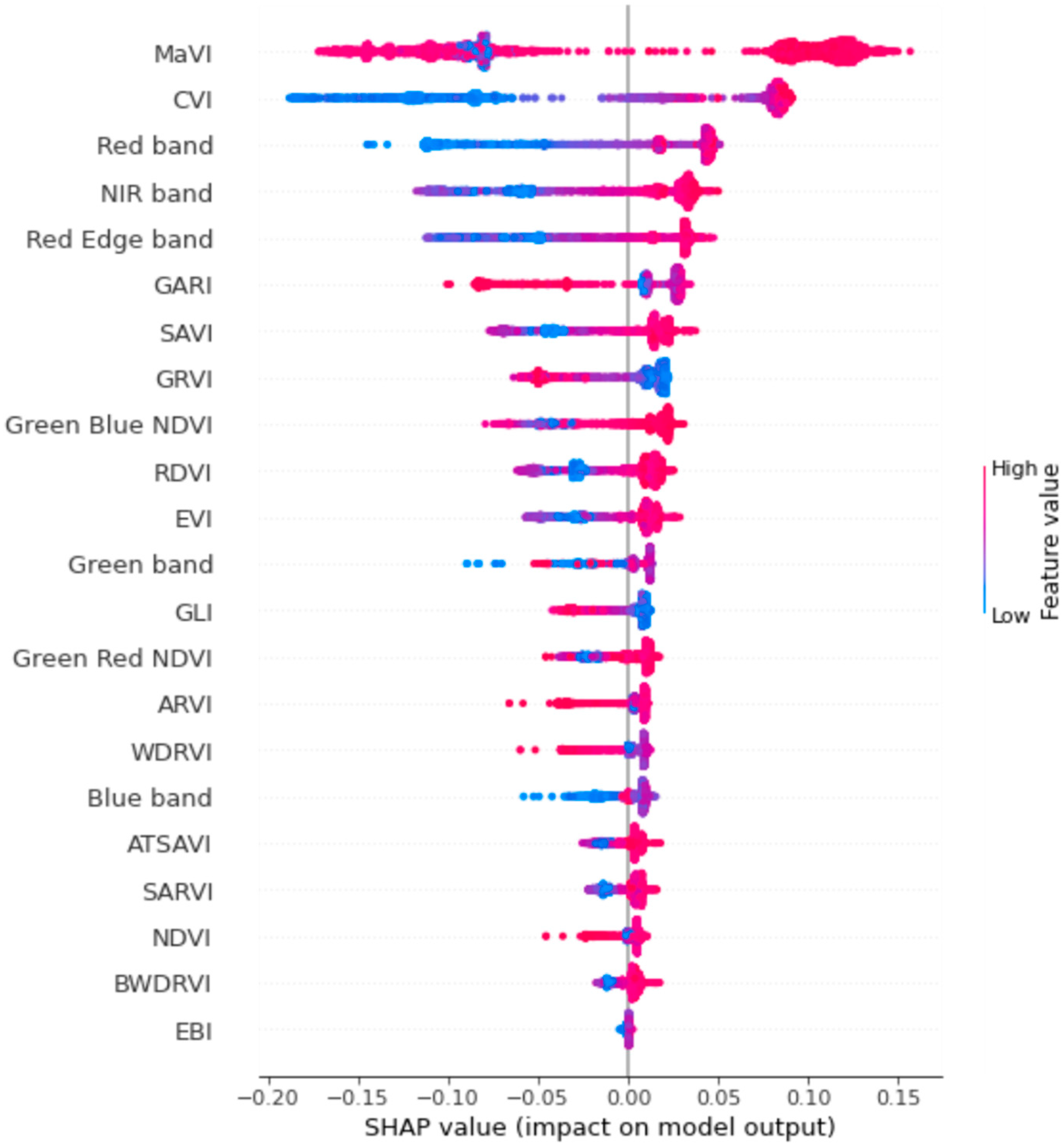
2.8. Feature Selection and Model Interpretation

In this study, we employed the concept of SHAP (Shapley additive explanations) values to fairly quantify the contribution of a feature to model predictions [44]. Using SHAP, we assessed the predictive capabilities of the given features to classify magenta-colored flowers (i.e., DM). The concept behind SHAP originated from Lloyd Shapley’s work on game theory [45] to assess the contribution of individual players, i.e., the dataset features, to a cooperative game, i.e., the model prediction. For the classification of each pixel (i.e., the model prediction), the marginal contribution of a feature (i.e., the SHAP value) is calculated by the weighted average of changes in model predictions for all possible feature permutations of a given dataset. We utilized the TreeExplainer [46] of the SHAP Python package to estimate the SHAP values of our model predictions. The model “payout” was the probability that a pixel was assigned to the DM-positive class. Using the classification test dataset, we created a SHAP beeswarm plot to visualize the global feature importance and to relate the importance ranking to the distribution of a feature. Based on this analysis we removed nonpredictive features from the training data and retrained the random forest model with the reduced dataset. After retraining, the model underwent a final classification accuracy assessment as described in the previous section. With the differences in accuracy measures before and after feature selection, we assessed the effect of the feature selection on the quality of the classification. Additionally, we created a change detection raster to quantitively derive and visualize the changes in pixel class assignments due to the feature selection.

2.9. Remote Sensing Plant Count Methodology

The goal of our study was to develop a remote-sensing-based DM mapping with results comparable to conventional field mappings, i.e., the number of plants per unit area. For this, we used a zonal statistics utility of pixel count per unit area, i.e., 1 m². To define the areal ratio between a DM inflorescence and a single image pixel, we assumed that one classified DM positive pixel represented one DM inflorescence (see Section 2.4).

We designed two separate zonal statistic aggregations: one for assessing the accuracy of the remote sensing plant count and another as a proposal for a remote sensing product for practical DM monitoring. For assessing the remote sensing plant count accuracy, we created a square buffer with a side length of 1 m around each GPS-logged in situ plant count (subsequently named the reference squares). We then counted all pixels classified as DM-positive in different counting settings, which we applied to optimize the remote sensing plant count against the in situ plant counts. The baseline setting simply counted all DM-positive pixels in each reference square. In all other counting settings, we applied a three-step filter approach with alternating thresholds before the remote sensing plant count. The filter approach was structured as follows:

• Polygonize DM positive pixel clusters (i.e., neighboring pixels) to vector image objects;
• Calculate a filter threshold for each image object on the basis of the most descriptive feature of the image classification;
• Remove all pixels below the threshold from the remote sensing plant count.

We tested different filter thresholds by calculating object-level percentiles in 10% steps starting at the 10% percentile and ending at the 90% percentile. Additionally, we tested the object-level mean as a filter. The quality of the remote sensing plant counts was determined by calculating the root-mean-square error (RMSE) between the remote sensing plant counts and the in situ plant counts. The best counting setting was defined by the smallest error value.

For practical DM monitoring, we applied a spatial aggregation approach. Contrary to the randomly chosen reference squares of our field campaign, we created a Universal Transverse Mercator polygon grid (EPSG: 32632) overlaying the study site, with the size of each grid cell being 1 m². The plant counting process remained the same as for the best remote sensing plant count counting setting.

3. Results

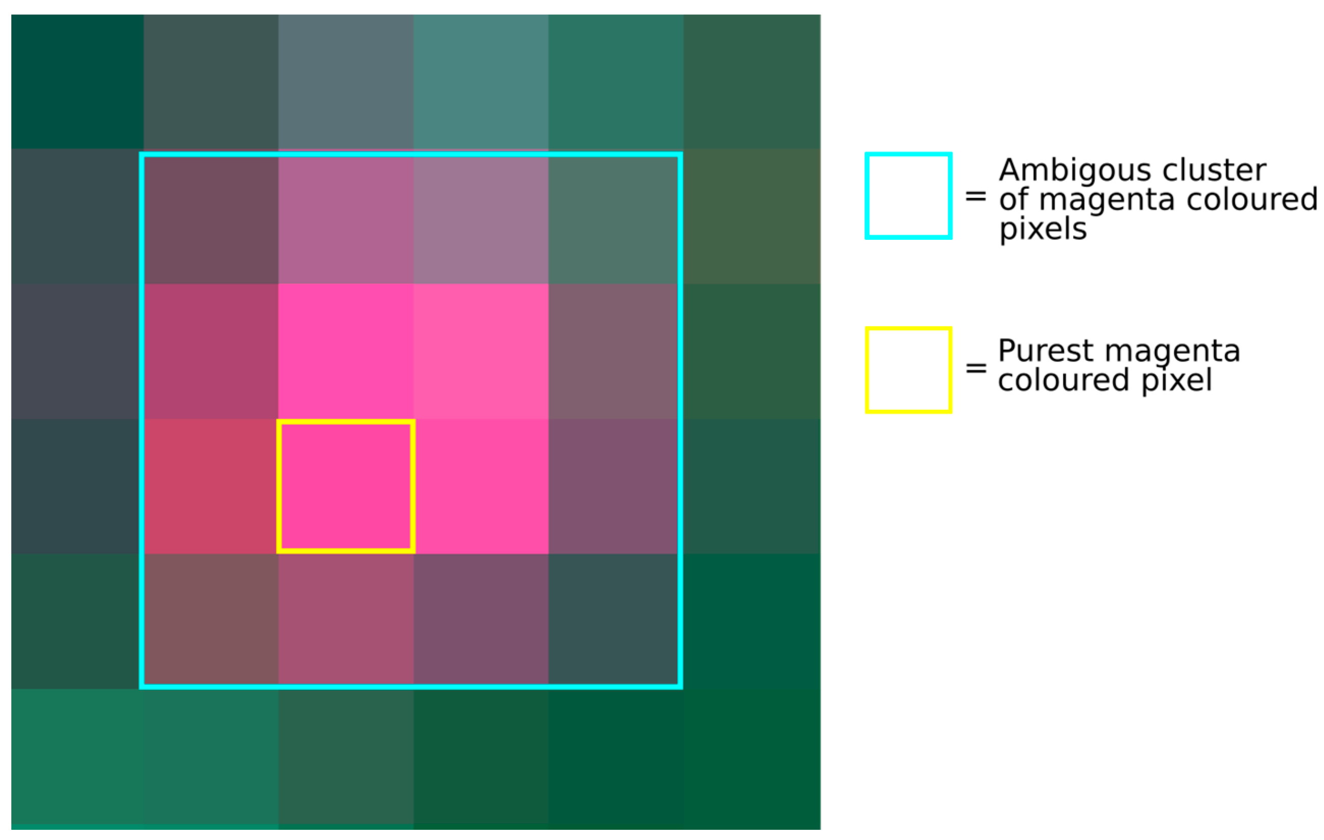
3.1. Ambiguity in the Drone Dataset

Difficulties arose during image interpretation as identifying the DM-positive class was shown to be ambiguous in some cases (Figure 4). Although, in theory, the inflorescence area of the target species is equal to or smaller than the spatial resolution of the drone dataset, in practice, multiple neighboring pixels may appear magenta-colored. Several factors may be responsible for this phenomenon:

• Mixed pixel phenomena, due to (1) a DM individual located at the common boundary of multiple pixels, (2) multiple DM individuals in direct proximity and partly occupy multiple neighboring pixels, or (3) DM individuals which did not grow perfectly straight and, therefore, appeared in neighboring pixels;
• Adjacency effects, i.e., the magenta flowers spectrally superimpose the neighboring pixels;
• Motion blur caused by camera movement during exposure;
• Keystone effect of the camera, which may cause a slight cross-track displacement.

Since we had no details about the camera calibration and were missing flight details of the drone survey, an in-depth discussion about potential influence factors seemed to be of limited use. We, therefore, decided to cope with the present data quality, which may lead to misclassification [47,48]. To minimize the number of false-positive labeled pixels in the reference data, we only used the purest magenta-colored pixel of a pixel cluster (i.e., the pixel with the highest surface reflectance in the blue and red bands). We assumed that these pixels most likely represented a DM individual. In contrast to the effect on false-positive labeling, the ambiguity problem is a minor advantage for avoiding false-negative labeling in the reference data. A pixel cluster clearly indicates the presence of magenta-colored vegetation; in contrast to pixel-based classifications, false negative labeling, therefore, is unlikely. For the DM-positive class, the reference dataset represented a characteristic value range of the data features, and some ambiguous pixels would most likely fall within these characteristic value ranges since pixels affected by the ambiguity problem still represented the underlying band relationship of magenta-colored vegetation.

3.2. Classification Results before Feature Selection

The accuracy assessment of the classification before the feature selection resulted in very high accuracy scores on the holdout dataset. We can report a precision score of 0.99, a recall score of 0.99, and an F1-score of 0.99. The accuracy scores suggest a nearly perfect differentiation of DM-positive and DM-negative classes. However, the high accuracy scores may be inflated due to this study’s sampling design. The sampling design for creating a labeled reference dataset, from which we derived the holdout dataset, was partially probabilistic and partially systematic, which may have inflated accuracy scores due to sample selection bias [48,49]. Moreover, the methodological drawback might harm the generalization potential of the accuracy assessment, since the holdout dataset does not necessarily represent the distribution of the underlying population [49]. A coping strategy for the latter would have been to add more labeled pixels to the reference dataset. However, we avoided implementing this strategy since the ambiguity problem limited our labeling capabilities. Additionally, adding more reference data would not have solved the sample selection bias problem, but may have even worsened it. For the quality assessment, however, we suggest that the limitations of the accuracy assessment played a minor role.

Due to the limitations of the quantitative accuracy assessment, the qualitative accuracy assessment became more important. The visual comparison suggested a noticeably good performance of the random forest model (Figure 5). Other than some rare outliers, magenta-colored pixels were reliably assigned to the DM-positive class. However, the results show that the classifier suffered from the ambiguity problem. Although the model was able to correctly assign the negative DM class to edge pixels of ambiguous pixels clusters, the class assignment appeared to be inconsistent.

In addition to the abovementioned restrictions, we identified leafless tree branches as a source of systematic false assignments of the DM-positive class. Spectra of tree branches showed similar reflectance curves to DM spectra with an almost constant reflectance level in the VIS; the reflectance in the NIR showed a similar steep increase in DM spectra. The high spectral similarities explain the misclassification.

3.3. Feature Selection and Predictive Performance of the MaVI

The feature with the highest impact was the MaVI (Figure 6). For the random forest model, the highest MaVI values corresponded to an increased probability of assigning the DM-positive class to a pixel. Furthermore, the small variation around 0 demonstrates the high impact of the MaVI for almost all model predictions. The MaVI’s high position in the feature importance ranking and the consistently high impact on model predictions support our hypothesis on the MaVI’s capabilities to detect magenta-colored vegetation.

In addition to the MaVI, all features up to rank 7 showed an observable impact on the random forest model to increase its predictive power (index abbreviations are listed in Table 1), i.e., CVI, the red band, the NIR band, the red-edge band, the GARI, and the SAVI. High reflectances in the NIR, red-edge, and red bands were associated with a higher probability of the DM-positive class. The latter turned out to be the key factor to differentiate magenta- and green-colored vegetation since the spectra showed the largest differences between the two land-cover types in this wavelength region. Vegetation indices such as the CVI and the GARI integrated the green and red bands. The CVI highlights the redness of a pixel, whereas the GARI highlights the greenness. Each, therefore, highlights the band relationship in the opposite extreme; higher CVI values and lower GARI values were often associated with an increase in prediction probability toward the DM-positive class. The SAVI increased the probability of a DM-positive class assignment in association with higher index values. We deduce that the model utilized the SAVI mainly for distinguishing between vegetated and nonvegetated pixels since a description of the green and red band relationship for distinguishing between magenta- and green-colored vegetation is missing in the index formula.

On the basis of our analysis of the beeswarm plot, we decided to reduce the model training dataset to the features with an observable impact on increasing the probability of predicting the DM-positive class. In summary, the reduced training dataset consisted of the following features: MaVI, CVI, the red band, the NIR band, the red-edge band, the GARI, and the SAVI.

3.4. Classification Result after Feature Selection

The accuracy assessment of the classification after feature selection still resulted in very high accuracy scores on the test dataset. We calculated a precision score of 0.99, a recall score of 0.99, and an F1-score of 0.99. Since the accuracy scores were identical for both classifications results, i.e., before and after feature selection, the former interpretation and discussion of the metrics are generally applicable to the latter classification accuracy scores. On the basis of the identical accuracy scores, we further deduce that the feature selection based on SHAP values was successful and that we correctly removed features with low predictive capabilities. To extrapolate the differences in class assignment to the entire drone dataset, we created a change detection raster that compares both classification results. By removing all features of low predictive power, the classification result for the entire dataset changed by a diminutive portion of 0.0002% of the total number of pixels (~73 million). The low percentage changes in the classification results of the entire drone dataset confirm that the dropped features had a negligible impact on the class assignment of the random forest model. We, therefore, propose that the interpretation and discussion of the former qualitative classification result assessment are generally applicable to the classification result of the entire dataset. A visual inspection of regions with class changes (Figure 5) revealed a slight improvement for ambiguous pixel clusters; some edge pixels of clusters were now assigned to the DM-negative class. It has to be noted, however, that the new class assignment was not consistent, and the ambiguity problem persisted for most of the medium- to large-sized clusters of the DM-positive class.

3.5. Remote Sensing Plant Count Accuracy Assessment

The remote sensing plant count accuracy assessment is summarized in

Table 2. Remote sensing plant count after applying different filter settings to the classification result.

In Situ	Without Filter	≥10% Percentile	≥20% Percentile	≥30% Percentile	≥40% Percentile	≥50% Percentile	≥60% Percentile	≥70% Percentile	≥80% Percentile	≥90% Percentile	Mean Filter
68	104	91	82	73	61	53	44	31	24	15	48
35	63	50	44	39	34	31	23	17	13	11	29
54	88	72	66	59	54	47	37	31	24	17	49
57	66	56	50	46	40	38	29	23	19	13	32
34	74	62	57	51	44	39	32	25	21	14	34
22	42	36	34	30	26	22	20	14	12	8	22
13	11	9	8	7	6	6	5	4	3	2	6
62	87	71	66	59	51	45	38	28	24	17	47
66	156	141	129	115	98	85	69	55	36	22	86
69	126	114	106	96	85	77	65	55	40	24	76

and

Table 3. Remote sensing plant count error metrics of different filter settings in comparison to the in situ plant counts.

Count Setting	RMSE
Without filter	42
≥10% percentile	31
≥20% percentile	26
≥30% percentile	19
≥40% percentile	14
≥50% percentile	12
≥60% percentile	16
≥70% percentile	23
≥80% percentile	29
≥90% percentile	37
Mean filter	13

. Counting all DM-positive pixels in the reference squares resulted in the highest error of all count settings (RMSE: 42 individuals per square meter). In nine out of 10 reference squares, the number of DM individuals was severely overestimated compared to the in situ plant count, with a mean relative overestimation of 76%. In the remaining reference square, the in situ plant count was underestimated by 17% by the baseline setting. We identified the ambiguity problem as the main cause of overestimation by comparing the classification result and the underlying drone dataset in the corresponding reference squares. Counting the pixels in a unit area is a direct aggregation of the classification results and, therefore, inherits the inflated number of DM-positive pixels in pixel clusters.

The overestimation outweighed the underestimation in terms of both the number of cases and the magnitude, and it accounted for the majority of the high error values of the baseline setting. We, therefore, applied an object-level threshold-based filter before counting to improve the error metric. We received the highest improvement by applying a median filter with an RMSE of 12 individuals per square meter, which is within the error margin stated by experts for a conventional plant survey. A similar error metric was achieved by an object-level mean filter with an RMSE of 13 individuals.

3.6. Assessing the Spatial Distribution and Abundance of Dactylorhiza majalis

In the open fen west of the linear trench, DM is widespread (Figure 7). We observed a north–south gradient of the DM population in terms of both spatial distribution and plant abundance. In the northern region of the open fen, DM formed large connected clusters with remote sensing plant counts ranging from five to over 100 DM individuals per square meter, whereas a remote sensing plant count per square meter lower than 50 predominated. However, multiple DM hotspots (remote sensing plant count per square meter >50) were present in the northern area of the open fen, noticeably forming adjacent clusters. In this part, we derived a maximum number of 164 DM individuals per square meter. In the southern part of the open fen, the size of connected DM clusters and the magnitude of DM individuals per square meter decreased. DM clusters were more sparsely spread than in the northern region. The remote sensing plant count ranged from five to 60 individuals, whereas the lower remote sensing plant count numbers predominated. The upper end of the remote sensing plant count range only occurred in a single square.

East of the beforementioned trench, only a single DM cluster with a remote sensing plant count ranging between five and 30 individuals per square meter existed. In the area which was subject to the forest fen removal in 2011, four squares above the lower display threshold existed. Two of these squares showed calibration targets for the drone during flight. For the remaining two squares, we were unable to derive a reliable explanation. From a visual inspection, the drone data indicated no DM pixels in the area. Considering the direct neighborhood of the squares, this observation is supported by the fact that the area was surrounded by water puddles and the squares were located at a considerable distance from the boundary of the former forest fen and the open fen. In particular, the latter indicated the absence of DM. The literature suggests that the majority of the DM diaspore is spread in direct proximity to its source, and that DM growth depends on the presence of mycorrhiza fungi in the soil [1], which limits the speed and distance of population spread. The MaVI, however, showed comparatively high index values, which may have been caused by leafless tree branches in these squares. However, since we are lacking in situ data for these specific locations, we are unable to exclude the possibility (although unlikely from an ecological perspective) that the DM population advanced toward the former forest fen area.

3.7. Relevance to Nature Conservation and Management

The study presented an approach to map DM abundance as an effective way of communicating results from a remote sensing-based analysis to a conservationist audience. Using drone data, conservationists can evaluate the success of conservation measures by introducing a comprehensive spatial perspective to a snapshot of the population development of DM. By aggregating plant individuals to a referenced grid, we paid special attention to assure reproducibility and extensibility of the presented approach. Therefore, the resulting map can be regarded as an initial state for long-term monitoring. By conducting the same analysis in subsequent years, an objective and spatially precise development of the DM population in our study site is possible.

In addition to the methodological advantages presented, using drones for plant surveys brings another benefit for nature conservation, i.e., it is possible to avoid plant damage caused by trampling. The surveyor only needs to enter the habitat to lay out or remove the calibration targets for the drone flight, which are generally located at the edges of an area of interest.

4. Conclusions

In this study, we developed and examined a drone-based approach to estimate the spatial distribution and abundance of DM in the Lehmkuhlen reservoir using very-high-spatial-resolution drone data. The results emphasize that our approach could produce valuable data on the status of a DM population during its flowering phase by highlighting the unique spectral response of magenta-colored vegetation. We integrated the spectral characteristics in our newly developed MaVI. A SHAP feature importance analysis of a random forest model demonstrated the strong performance of MaVI in identifying DM. In addition to MaVI, the most suitable features were the NIR/red and the green/red band combinations. We, therefore, recommend integrating the MaVI, the CVI, and the GARI to reliably classify the presence of DM. However, in this study, transferring the classification result to a remote sensing plant count given the available data was limited due to the presence of image artefacts which we summarized under the term ambiguity problem. We tried to cope with the ambiguity problem by optimizing the remote sensing plant count against in situ plant counts via the application of a post-classification median filter on an image object level to reduce the RMSE. The error metrics indicated a noticeable improvement, while a visual inspection of the filtered classification results revealed that the ambiguity problem persisted. Consequently, the ability of this approach to accurately estimate plant counts is limited by its underlying assumption that one pixel indicates one plant individual. Nevertheless, our approach can supplement monitoring programs with information on plant count with acceptable accuracy to address data scarcity. Additionally, our approach can extend the DM monitoring by assessing the spatial distribution of a plant population, representing a step forward from simple plant counts to indicate the success of conservation measures.

References

1. Dullau, S.; Richter, F.; Adert, N.; Meyer, M.H.; Hensen, H.; Tischew, S. Handlungsempfehlung zur Populationsstärkung und Wiederansiedlung von Dactylorhiza majalis am Beispiel des Biosphärenreservat Karstlandschaft Südharz; Hochschule Anhalt: Bernburg, Germany, 2019. [Google Scholar] [CrossRef]
2. Lohr, M.; Margenburg, B. Das Breitblättrige Knabenkraut Dactylorhiza majalis–Orchidee des Jahres 2020. J. Eur. Orchid. 2020, 52, 287–323. [Google Scholar]
3. Gregor, T.; Saurwein, H.-P. Wer erhält das Großblättrige Knabenkraut (Dactylorhiza majalis). Beitr. Naturkunde Osthess. 2010, 47, 3–6. [Google Scholar]
4. Messlinger, U.; Pape, T.; Wolf, S. Erhaltungsstrategien für das Breitblättrige Knabenkraut (Dactylorhiza majalis) in Stadt und Landkreis Ansbach. Regnitz Flora 2018, 9, 82–106. [Google Scholar]
5. Wotavová, K.; Balounová, Z.; Kindlmann, P. Factors Affecting Persistence of Terrestrial Orchids in Wet Meadows and Implications for Their Conservation in a Changing Agricultural Landscape. Biol. Conserv. 2004, 118, 271–279. [Google Scholar] [CrossRef]
6. Reinhard, H.R.; Gölz, P.; Peter, R.; Wildermuth, H. Die Orchideen der Schweiz und Angrenzender Gebiete; Fotorotar AG: Egg, Switzerland, 1991. [Google Scholar] [CrossRef]
7. Pettorelli, N.; Safi, K.; Turner, W. Satellite Remote Sensing, Biodiversity Research and Conservation of the Future. Philos. Trans. R. Soc. B 2014, 369, 20130190. [Google Scholar] [CrossRef]
8. Horton, R.; Cano, E.; Bulanon, D.; Fallahi, E. Peach Flower Monitoring Using Aerial Multispectral Imaging. J. Imaging 2017, 3, 2. [Google Scholar] [CrossRef]
9. Fang, S.; Tang, W.; Peng, Y.; Gong, Y.; Dai, C.; Chai, R.; Liu, K. Remote Estimation of Vegetation Fraction and Flower Fraction in Oilseed Rape with Unmanned Aerial Vehicle Data. Remote Sens. 2016, 8, 416. [Google Scholar] [CrossRef] [Green Version]
10. Abdel-Rahman, E.; Makori, D.; Landmann, T.; Piiroinen, R.; Gasim, S.; Pellikka, P.; Raina, S. The Utility of AISA Eagle Hyperspectral Data and Random Forest Classifier for Flower Mapping. Remote Sens. 2015, 7, 13298–13318. [Google Scholar] [CrossRef] [Green Version]
11. Hassan, N.; Numata, S.; Hosaka, T.; Hashim, M. Remote Detection of Flowering Somei Yoshino (Prunus × yedoensis ) in an Urban Park Using IKONOS Imagery: Comparison of Hard and Soft Classifiers. J. Appl. Remote Sens. 2015, 9, 096046. [Google Scholar] [CrossRef]
12. Sulik, J.J.; Long, D.S. Spectral Indices for Yellow Canola Flowers. Int. J. Remote Sens. 2015, 36, 2751–2765. [Google Scholar] [CrossRef]
13. Landmann, T.; Piiroinen, R.; Makori, D.M.; Abdel-Rahman, E.M.; Makau, S.; Pellikka, P.; Raina, S.K. Application of Hyperspectral Remote Sensing for Flower Mapping in African Savannas. Remote Sens. Environ. 2015, 166, 50–60. [Google Scholar] [CrossRef]
14. Carl, C.; Landgraf, D.; van der Maaten-Theunissen, M.; Biber, P.; Pretzsch, H. Robinia Pseudoacacia L. Flower Analyzed by Using An Unmanned Aerial Vehicle (UAV). Remote Sens. 2017, 9, 1091. [Google Scholar] [CrossRef] [Green Version]
15. Roosjen, P.; Suomalainen, J.; Bartholomeus, H.; Clevers, J. Hyperspectral Reflectance Anisotropy Measurements Using a Pushbroom Spectrometer on an Unmanned Aerial Vehicle—Results for Barley, Winter Wheat, and Potato. Remote Sens. 2016, 8, 909. [Google Scholar] [CrossRef] [Green Version]
16. Severtson, D.; Callow, N.; Flower, K.; Neuhaus, A.; Olejnik, M.; Nansen, C. Unmanned Aerial Vehicle Canopy Reflectance Data Detects Potassium Deficiency and Green Peach Aphid Susceptibility in Canola. Precis. Agric. 2016, 17, 659–677. [Google Scholar] [CrossRef] [Green Version]
17. Valente, J.; Sari, B.; Kooistra, L.; Kramer, H.; Mücher, S. Automated Crop Plant Counting from Very High-Resolution Aerial Imagery. Precis. Agric. 2020, 21, 1366–1384. [Google Scholar] [CrossRef]
18. Shen, M.; Chen, J.; Zhu, X.; Tang, Y. Yellow Flowers Can Decrease NDVI and EVI Values: Evidence from a Field Experiment in an Alpine Meadow. Can. J. Remote Sens. 2009, 35, 8. [Google Scholar] [CrossRef]
19. Shen, M.; Chen, J.; Zhu, X.; Tang, Y.; Chen, X. Do Flowers Affect Biomass Estimate Accuracy from NDVI and EVI? Int. J. Remote Sens. 2010, 31, 2139–2149. [Google Scholar] [CrossRef]
20. Verma, K.S.; Saxena, R.K.; Hajare, T.N.; Kharche, V.K.; Kumari, P.A. Spectral Response of Gram Varieties under Variable Soil Conditions. Int. J. Remote Sens. 2002, 23, 313–324. [Google Scholar] [CrossRef]
21. Chen, B.; Jin, Y.; Brown, P. An Enhanced Bloom Index for Quantifying Floral Phenology Using Multi-Scale Remote Sensing Observations. ISPRS J. Photogramm. Remote Sens. 2019, 156, 108–120. [Google Scholar] [CrossRef]
22. Seer, F.K.; Schrautzer, J. Status, Future Prospects, and Management Recommendations for Alkaline Fens in an Agricultural Landscape: A Comprehensive Survey. J. Nat. Conserv. 2014, 22, 358–368. [Google Scholar] [CrossRef]
23. Schrautzer, J.; Trepel, M. Niedermoore im Östlichen Hügelland-Lehmkuhlener Stauung. Tuexenia Mitt. Florist. Soziol. Arb. 2014, 7, 47–49. [Google Scholar]
24. MELUND. Erhaltungsziele für das Gesetzlich Geschützte Gebiet von Gemeinschaftlicher Bedeutung DE-1728-303 “Lehmkuhlener Stauung”; Amtsblatt für Schleswig Holstein; Ministerium für Energiewende, Landwirtschaft, Umwelt, Natur und Digitalisierung (MELUND): Kiel, Germany, 2016; p. 1033. [Google Scholar]
25. Wingtra AG. Wingtra One—Technical Specifications; Wingtra AG: Zurich, Switzerland, 2021; Available online: https://wingtra.com/wp-content/uploads/Wingtra-Technical-Specifications.pdf (accessed on 12 July 2022).
26. MicaSense, Inc. MicaSense Altum—Specifications; MicaSense, Inc.: Seattle, WA, USA, 2020; Available online: https://1w2yci3p7wwa1k9jjd1jygxd-wpengine.netdna-ssl.com/wp-content/uploads/2022/03/Altum-PT-Specification-Table-Download.pdf (accessed on 12 July 2022).
27. Tremp, H. Aufnahme und Analyse Vegetationsökologischer Daten-Kapitel 3: Datenaufnahme, 1st ed.; utb GmbH: Stuttgart, Germany, 2005; ISBN 978-3-8385-8299-3. [Google Scholar]
28. Maxwell, A.E.; Warner, T.A.; Fang, F. Implementation of Machine-Learning Classification in Remote Sensing: An Applied Review. Int. J. Remote Sens. 2018, 39, 2784–2817. [Google Scholar] [CrossRef] [Green Version]
29. Kaufman, Y.J.; Tanre, D. Atmospherically Resistant Vegetation Index (ARVI) for EOS-MODIS. IEEE Trans. Geosci. Remote Sens. 1992, 30, 261–270. [Google Scholar] [CrossRef]
30. Frederic, B.; Guyot, G. Potential and Limitations of Vegetation Indices for LAI and APAR Assessment. Remote Sens. Environ. 1991, 104, 88–95. [Google Scholar]
31. Hancock, D.W.; Dougherty, C.T. Relationships between Blue- and Red-based Vegetation Indices and Leaf Area and Yield of Alfalfa. Crop Sci. 2007, 47, 2547–2556. [Google Scholar] [CrossRef]
32. Vincini, M.; Frazzi, E.; D’Alessio, P. A Broad-Band Leaf Chlorophyll Vegetation Index at the Canopy Scale. Precis. Agric. 2008, 9, 303–319. [Google Scholar] [CrossRef]
33. Huete, A.; Justice, C.; van Leeuwen, W. MODIS VEGETATION INDEX (MOD 13) ALGORITHM THEORETICAL BASIS DOCUMENT, VERSION 3. 1999. Available online: https://modis.gsfc.nasa.gov/data/atbd/atbd_mod13.pdf (accessed on 12 July 2022).
34. Gitelson, A.A.; Kaufman, Y.J.; Merzlyak, M.N. Use of a Green Channel in Remote Sensing of Global Vegetation from EOS-MODIS. Remote Sens. Environ. 1996, 58, 289–298. [Google Scholar] [CrossRef]
35. Gobron, N.; Pinty, B.; Verstraete, M.M.; Widlowski, J.-L. Advanced Vegetation Indices Optimized for Up-Coming Sensors: Design, Performance, and Applications. IEEE Trans. Geosci. Remote Sens. 2000, 38, 2489–2505. [Google Scholar] [CrossRef]
36. Wang, B.; Huang, J.; Tang, Y.; Wang, X. New Vegetation Index and Its Application in Estimating Leaf Area Index of Rice. Rice Sci. 2007, 14, 195–203. [Google Scholar] [CrossRef]
37. Motohka, T.; Nasahara, K.; Hiroyuki, O.; Satoshi, T. Applicability of Green-Red Vegetation Index for Remote Sensing of Vegetation Phenology. Remote Sens. 2010, 2, 2369. [Google Scholar] [CrossRef] [Green Version]
38. Rouse, J.W.; Haas, R.H.; Deering, D.W.; Schell, J.A.; Harlan, J.C. Monitoring the Vernal Advancement and Retrogradation (Green Wave Effect) of Natural Vegetation. [Great Plains Corridor]. 1973. Available online: https://ntrs.nasa.gov/citations/19730017588 (accessed on 12 July 2022).
39. Roujean, J.-L.; Breon, F.-M. Estimating PAR Absorbed by Vegetation from Bidirectional Reflectance Measurements. Remote Sens. Environ. 1995, 51, 375–384. [Google Scholar] [CrossRef]
40. Gitelson, A.A. Wide Dynamic Range Vegetation Index for Remote Quantification of Biophysical Characteristics of Vegetation. J. Plant Physiol. 2004, 161, 165–173. [Google Scholar] [CrossRef] [PubMed] [Green Version]
41. Breiman, L. Random Forests. Mach. Learn. 2001, 45, 5–32. [Google Scholar] [CrossRef] [Green Version]
42. Pedregosa, F.; Varoquaux, G.; Gramfort, A.; Michel, V.; Thirion, B.; Grisel, O.; Blondel, M.; Prettenhofer, P.; Weiss, R.; Dubourg, V.; et al. Scikit-Learn: Machine Learning in Python. J. Mach. Learn. Res. 2011, 12, 2825–2830. [Google Scholar]
43. Belgiu, M.; Drăguţ, L. Random Forest in Remote Sensing: A Review of Applications and Future Directions. ISPRS J. Photogramm. Remote Sens. 2016, 114, 24–31. [Google Scholar] [CrossRef]
44. Lundberg, S.; Lee, S.-I. A Unified Approach to Interpreting Model Predictions. arXiv 2017, arXiv:1705.07874. [Google Scholar]
45. Shapley, L.S. 17. A Value for n-Person Games. In Contributions to the Theory of Games (AM-28); Kuhn, H.W., Tucker, A.W., Eds.; Princeton University Press: Princeton, NJ, USA, 1953; Volume II, pp. 307–318. [Google Scholar]
46. Lundberg, S.M.; Erion, G.; Chen, H.; DeGrave, A.; Prutkin, J.M.; Nair, B.; Katz, R.; Himmelfarb, J.; Bansal, N.; Lee, S.-I. From Local Explanations to Global Understanding with Explainable AI for Trees. Nat. Mach. Intell. 2020, 2, 56–67. [Google Scholar] [CrossRef]
47. Guo, Q.; Li, W.; Liu, D.; Chen, J. A Framework for Supervised Image Classification with Incomplete Training Samples. Photogramm. Eng. Remote Sens. 2012, 78, 595–604. [Google Scholar] [CrossRef]
48. Stehman, S.V. Sampling Designs for Accuracy Assessment of Land Cover. Int. J. Remote Sens. 2009, 30, 5243–5272. [Google Scholar] [CrossRef]
49. Waldner, F. The T Index: Measuring the Reliability of Accuracy Estimates Obtained from Non-Probability Samples. Remote Sens. 2020, 12, 2483. [Google Scholar] [CrossRef]
Figure 1. (a) Overview of the Lehmkuhlen reservoir; (b) location of the study area in Germany; (c) photograph illustrating the abundance of Dactylorhiza majalis during drone flight; (d) close-up picture of a Dactylorhiza majalis inflorescence.
Drones 06 00174 g001
Figure 2. Methodological workflow of this study: from data acquisition to mapping result.
Drones 06 00174 g002
Figure 3. Mean spectra of different landcover types sampled from the drone dataset.
Drones 06 00174 g003
Figure 4. True color band combination illustrating the ambiguity problem. A common case in the dataset, where we could not unambiguously identify the most likely pixel representing a Dactylohriza majalis individual.
Drones 06 00174 g004
Figure 5. Comparison between the true color image and the random forest classification results before and after feature selection. The figure illustrates the reliable performance of the classifier to identify magenta-colored vegetation. The figure additionally illustrates the change in classification results due to the SHAP value feature selection.
Drones 06 00174 g005
Figure 6. Overall feature importance for predicting the Dactylorhiza majalis-positive class. Note that the magenta vegetation index value range is skewed toward high negative values, whereas the continuous color scale of the beeswarm plot also colors negative high impact values in a shade of red. Index abbreviations are listed in Table 1.
Drones 06 00174 g006
Figure 7. Aggregated Dactylorhiza majalis individuals per square meter based on the median filtered remote sensing plant count.
Drones 06 00174 g007