Abstract
3D building models are widely used in many applications. The traditional image-based 3D reconstruction pipeline without using semantic information is inefficient for building reconstruction in rural areas. An oblique view selection methodology for efficient and accurate building reconstruction in rural areas is proposed in this paper. A Mask R-CNN model is trained using satellite datasets and used to detect building instances in nadir UAV images. Then, the detected building instances and UAV images are directly georeferenced. The georeferenced building instances are used to select oblique images that cover buildings by using nearest neighbours search. Finally, precise match pairs are generated from the selected oblique images and nadir images using their georeferenced principal points. The proposed methodology is tested on a dataset containing 9775 UAV images. A total of 4441 oblique images covering 99.4% of all the buildings in the survey area are automatically selected. Experimental results show that the average precision and recall of the oblique view selection are 0.90 and 0.88, respectively. The percentage of robustly matched oblique-oblique and oblique-nadir image pairs are above 94% and 84.0%, respectively. The proposed methodology is evaluated for sparse and dense reconstruction. Experimental results show that the sparse reconstruction based on the proposed methodology reduces 68.9% of the data processing time, and it is comparably accurate and complete. Experimental results also show high consistency between the dense point clouds of buildings reconstructed by the traditional pipeline and the pipeline based on the proposed methodology.
1. Introduction
3D building models have been widely used in many applications including city modelling and simulation [1,2], civil infrastructure monitoring [3], disaster management and emergency response [4,5,6,7], cultural heritage conservation [8], etc. In recent years, oblique photogrammetry based on aerial images acquired by an Unmanned Aerial Vehicle (UAV) has become one of the mainstream solutions to 3D reconstruction of photorealistic 3D building models due to its cost-effectiveness and convenience [9,10,11,12,13]. A commonly used image-based 3D reconstruction pipeline mainly consists of image matching, image orientation, dense matching, mesh construction, and texture mapping. Image matching extracts feature points from images and finds initial tie points between images based on similarity measures [14,15,16]. Geometrically consistent tie points are then selected from the initial tie points based on the fundamental matrix with random sample consensus (RANSAC) loops [17,18]. Image orientation solves the optimal position and orientation of each image based on the geometrically consistent tie points. Structure from motion (SfM) is commonly used for fully automatic image orientation [19,20,21,22,23]. Dense matching finds dense correspondence between images and generates dense depth maps [24,25,26]. Mesh construction builds a geometric model of the scene using 3D triangles [27]. Additionally, texture mapping maps 2D texture onto the 3D mesh model. In this pipeline, the latter procedures depend on the former ones. Image matching and SfM reconstruction significantly affect the accuracy, robustness and efficiency of the pipeline.
Although the abovementioned image-based 3D reconstruction pipeline works well in modelling buildings in urban areas, problems are encountered when this pipeline is used for building reconstruction in rural areas. First, image matching and SfM reconstruction using all the acquired images are inefficient for building reconstruction in rural areas. Building density is high in urban areas, and each single oblique image covers buildings and provides valuable observations. Therefore, each image is necessary for building reconstruction. In contrast, building density in rural areas is usually much lower than that in urban areas, and a considerable proportion of aerial images acquired in rural areas do not cover any buildings. The aerial images that do not cover buildings are unnecessary for building reconstruction. In this situation, reconstruction of buildings using all the acquired images is inefficient, especially for time-critical applications. Second, aerial images with repetitive textures are prone to mismatch [28]. Rural areas are commonly covered by farmland, vegetation and bare earth. Aerial images acquired in these areas have repetitive textures. Feature points extracted from these images are less distinctive and prone to mismatch, which undermines the accuracy and robustness of reconstruction.
The problems can be solved by selecting the images that cover buildings and robust matching the selected images. The semantic information embedded in the images is the key to the selection of building-covering images. In recent years, deep learning has been widely used for extracting semantic information from remote sensing imagery [29,30,31]. The extraction of building information from aerial and satellite images has been intensively studied based on deep learning methods. Pixels pertaining to buildings have been extracted using semantic segmentation based on models like fully convolutional network (FCN), U-Net and their variants [32,33,34]. Outlines of buildings have been delineated based on the extracted pixels pertaining to buildings [35,36,37]. Building instances have been detected using instance segmentation based on models like U-Net, Mask R-CNN and their variants [38]. On the basis of instance segmentation, semantic information about building area, building change detection and building types has been extracted [39,40,41]. Although rich information about buildings can be extracted from imagery using deep learning methods, the problems posed above cannot be solved by simply using deep learning. Collecting and labelling the dataset is time-consuming and introduces computational overhead to the existing 3D reconstruction pipeline, which is impractical for time-critical applications.
Researchers in the photogrammetry community have proposed methodologies for incorporating semantic information in the photogrammetric pipeline [42,43,44,45]. Research works on improving photogrammetric tasks using semantic information have been reported. Stathopoulou and Remondino improved feature point matching and dense matching results based on semantic segmentation [46]. A fully convolutional network was used to classify pixels of an image to sky, building, window and obstacle. The feature point matching and dense matching were constrained in the image regions pertaining to buildings. Stathopoulou et al. proposed a novel approach to depth estimation of textureless image areas by leveraging semantic priors [47]. Semantic labels were used to impose constraints on image pixels during multi-view stereo, which improved the depth estimation in textureless areas. Zhou et al. proposed a method for selecting building facade texture images from abundant oblique images based on building models of an urban area [48]. Experimental results showed that optimal texture images could be selected using semantic information embedded in building models and a large amount of computation time and space could be saved. Yu et al. proposed a fully automatic method for reconstruction of prismatic building models with flat roofs from multi-view aerial images [49]. The proposed method conducted building segmentation using the digital surface model and digital orthophoto map. Building outlines were extracted based on the segmentation map. Building height was estimated based on the extracted outlines, and individual building models were generated. Yang et al. proposed a method to remove the influence of moving cars on 3D modelling of an urban area using instance segmentation [50]. The proposed method detected cars from oblique images using Mask R-CNN. Geometric deformation and error texture mapping problems were solved based on the analysis of image patches corresponding to the detected cars. Oniga et al. provided an end-to-end pipeline for reconstruction of building models from oblique UAV images [51]. The proposed method generated a dense cloud of an urban area based on the traditional SfM-based photogrammetric pipeline. The generated dense cloud was then used for the extraction of above-ground points using a filtering algorithm. The above-ground points were classified to vegetation, building, civil infrastructure and cars using a random forest algorithm, and building models were finally derived from the building points.
Although the above-mentioned research works made significant progresses in improving photogrammetric tasks using semantic information, most of these works were still based on the traditional SfM-based photogrammetric pipeline and focused on the 3D reconstruction of buildings in the urban scenario. In this paper, a methodology is proposed for efficient and accurate building reconstruction in rural areas. The methodology effectively selects oblique images that cover buildings by using semantic and spatial information, and it improves the efficiency of image matching and SfM reconstruction processes. Section 2 details the workflow and procedures of the proposed methodology. Experimental results are provided in Section 3. Discussions and analysis of the proposed methodology and the results are made in Section 4. Conclusions are made in Section 5.
2. Methodology
The workflow of the proposed methodology is illustrated in Figure 1. First, a Mask R-CNN model is trained using satellite datasets. Then, UAV images and POS (Position and Orientation System) observations are acquired in an aerial survey. Thirdly, building instances are detected in nadir images using the trained Mask R-CNN model. The detected building instances and the UAV images are directly georeferenced. Fourthly, the georeferenced building points are used to select oblique images that cover buildings by using nearest neighbours search. Finally, match pairs are generated from the nadir images and the selected oblique images using the georeferenced principal points. In a standard reconstruction pipeline, the generated match pairs are used for pairwise image matching to find tie points between images. Then a SfM reconstruction is conducted based on the tie points.
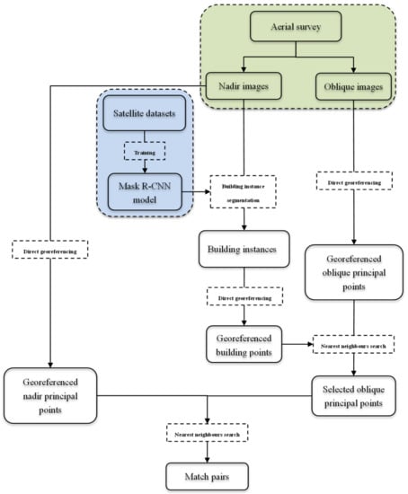
Figure 1.
Workflow of the proposed methodology. The light green color represents the field work for data acquisition; the light blue color represents the work for data preprocessing and model training.
2.1. Building Detection in Nadir Images Based on Mask R-CNN
A Mask R-CNN model is trained before an aerial survey and then used to detect buildings in nadir UAV images. The Mask R-CNN is trained using satellite datasets instead of the acquired UAV images to save data processing time. The satellite datasets used for the model training consist of an open dataset and a dataset of the survey area. The open dataset is used to accelerate the model training process based on transfer learning. The dataset of the survey area is manually labelled and used to improve the performance of the model.
The trained Mask R-CNN model detects building instances in nadir UAV images at pixel level and delineates their shapes. It provides three outputs for each building instance: a bounding box, a confidence score, and a mask. A bounding box represents the outmost boundary of a building instance. The confidence score of a building instance represents its quality of classification. And the quality of detected building instances significantly influences the quality of oblique view selection. A threshold for confidence score is used to determine valid building instances. To set the value of the threshold, the relationship between the confidence score and view selection is investigated using the nadir images. The ground truth for the evaluation of view selection is prepared by a human operator. The human operator manually selects the images that cover buildings from UAV images. An image is selected as long as it covers more than a part of a building. The precision, recall, accuracy and F1 score are used to evaluate the result of the view selection (Equations (1)–(4)).
where TP is defined as the number of selected images that truly cover buildings; FP is the number of selected images that do not cover any buildings; TN is the number of images that are not selected and do not cover any buildings; and FN is the number of images that are not selected but truly cover buildings.
2.2. DEM-aided Direct Georeferencing of Valid Building Instances and UAV Images
Oblique view selection is based on the ground position of the valid building instances and the UAV images. The ground position of the valid building instances and the UAV images is solved using the DEM-aided direct georeferencing algorithm proposed in [52]. The DEM-aided direct georeferencing of an image point is based on the inverse form of the Collinearity Equations as follows.
where is the spatial position of the ground point corresponding to the image point under the object coordinate system; is the position of the image point under the image plane coordinate system; is the spatial position of the projection center under the object coordinate system; is the focal length; and to are the elements of the absolute rotation matrix from the image coordinate system to the object coordinate system defined as
For DEM-aided direct georeferencing of a valid building instance, the position of the valid building instance under the image plane coordinate system is required. In this work, the position of a building instance is represented by the center of the bounding box predicted by the Mask R-CNN model. As the position of a predicted bounding box is under the pixel coordinate system of an image tile, the position of a building instance is transformed from the pixel coordinate system of an image tile, over the pixel coordinate system of a UAV image to the image plane coordinate system.
In this work, the ground position of an image is represented by the ground position of its principal point. For DEM-aided direct georeferencing of a principal point, its position under the image plane coordinate system is required. The principal point of an image is the origin of the image plane coordinate system. Therefore, (0,0) is used as the position of the principal point for DEM-aided direct georeferencing of an image.
DEM-aided direct georeferencing of a valid building instance and a UAV image is dependent on the absolute rotation matrix of the corresponding image. Assume an oblique imaging system consisting of five cameras facing backward, forward, right, left and nadir; the absolute rotation matrix of an image is calculated as follows. The absolute rotation matrix of a nadir image is calculated using the POS observations based on the method proposed in [53]. The absolute orientation matrix of an oblique image is calculated according to Equation (8).
where is the absolute rotation matrix of the simultaneously exposed nadir image and is the relative rotation matrix from the nadir camera to the corresponding oblique camera. If the installation angles of all cameras are precisely available, the relative rotation matrix of each oblique camera can be directly calculated. If the installation angles are unavailable, the relative rotation matrices can be estimated by camera system calibration using an image set. In this work, the East-North-Up (ENU) coordinate system is used as the object coordinate system. The spatial position of a projection center is approximated using the camera exposure position which is transformed from the geodetic coordinate system to the ENU coordinate system.
2.3. Oblique View Selection and Match Pair Generation Based on Nearest Neighbours Search
Given the ground position of valid building instances and UAV images, oblique images are selected based on nearest neighbours search. Figure 2 illustrates the principle of oblique view selection. In this figure, and are two images that cover an area on the ground. is an oblique image and is a nadir image. and are the project centers of and , respectively. covers a building and the corresponding building instance is detected in the image at point b. B is a building point corresponding to b and located by direct georeferencing. pp is the principal point of . PP is a georeferenced principal point corresponding to pp and located by direct georeferencing. The red line shows the horizontal view of a search circle centered at PP. The radius of the search circle is R. The search circle of an oblique image corresponds to a field of view of the image. An oblique image is selected as long as a georeferenced building point exists within the search circle of the image, which is implemented using nearest neighbours search. The nearest neighbours search is based on a k-d tree which is constructed from the georeferenced building points. For each oblique image, building points are searched within its search circle using the k-d tree. If a georeferenced building point is searched, the oblique image is selected.
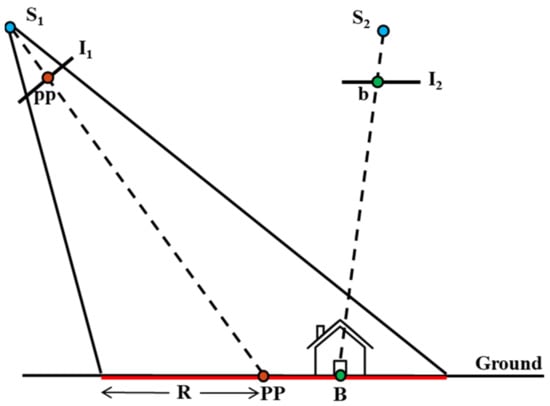
Figure 2.
Illustration of oblique view selection.
After the oblique images covering buildings are selected, match pairs are generated from the selected oblique images and all the nadir images. A satisfactory match pair consists of two overlapping images that can be robustly matched. For an oblique imaging system consisting of five cameras facing backward, forward, right, left and nadir, match pairs are generated in sequence as follows. First, for each oblique image, overlapping images are searched among images from the same oblique camera, the oblique camera facing the opposite direction and the nadir camera. Second, for each nadir image, overlapping images are searched among other nadir images. For example, for an image from the backward-looking camera, overlapping images are searched among images from the backward-looking camera, the forward-looking camera and the nadir camera, respectively. Figure 3 illustrates searching overlapping images for an image i from the backward-looking camera. From left to right overlapping images are searched from among backward-looking images, forward-looking images and nadir images, respectively. Small circles in the figure denote the georeferenced principal points. Solid arrows denote viewing directions of images. In the first case shown by Figure 3a, all of the images are from the backward-looking camera. The images in the central strip look in the same direction as image i, and the images in the neighbouring strips look in the opposite direction. Therefore, neighbouring images in the same strip as image i are considered as overlapping images of image i in this case. In the second case shown by Figure 3b, the forward-looking images in the same strip as image i look in the opposite direction of image i, and the images in the neighbouring strips look in the same direction as image i. In this case, the overlapping images are searched within a circle based on nearest neighbours search. The nearest neighbours search is conducted using the k-d tree constructed from the georeferenced principal points of the forward-looking images and a given radius r. The searched images that look in the opposite direction of image i are removed using viewing direction filtering. The viewing direction of an image is the direction of the vector from its projection center to its georeferenced principal point. A searched image is removed if the difference between the viewing directions of the image and image i is larger than a given threshold . In the third case shown by Figure 3c, all the nadir images look vertically down. The overlapping images are searched within a circle based on nearest neighbours search using the k-d tree constructed from the georeferenced principal points of the nadir images.
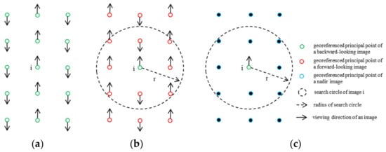
Figure 3.
Illustration of searching overlapping images for a backward-looking image from: (a) backward-looking images; (b) forward-looking images; (c) nadir images.
For a nadir image, overlapping images are searched among other nadir images, which is similar to the case illustrated by Figure 3c. However, no viewing direction filtering is done as all the images look vertically down.
The number of match pairs influences the time efficiency of pairwise image matching. To reduce the time cost of pairwise image matching, the number of match pairs is constrained for an image. Specifically, for an oblique image, the numbers of match pairs in the first, the second and the third case are k1, k2 and k3, respectively. For a nadir image, the number of match pairs is k4. Furthermore, to connect nadir images from neighbouring strips, k4/2 images are selected from the same strip and k4/2 images are selected from the neighbouring strips. To generate the given number of match pairs for an image, the searched overlapping images are sorted in ascending order based on the distance between them and the image. The given number of match pairs are selected from the candidates at the front of the sorted array.
3. Experimental Results
A large-scale UAV image set acquired over a rural area was used to evaluate the performance of the proposed methodology. First, the specification of the acquired data is detailed. Second, the results of model training and building detection in nadir images are provided. Third, the direct-georeferenced valid building instances and UAV images are illustrated. Finally, evaluations of the selected oblique images and the generated match pairs are provided. Sparse and dense reconstructions based on the proposed methodology and the traditional pipeline were compared. All of the experiments were performed on a Dell Precision Tower 7810 workstation. The workstation is equipped with a Windows 10 Professional operating system, an Intel Xeon E5-2630 CPU, a NVIDIA Quadro M4000 GPU and 128 GB memory.
3.1. Survey Area and Data Specification
Figure 4 shows an orthophoto of the survey area. The survey area is 5.2 km from east to west and 4.1 km from south to north. The elevation of the survey area is about 65 m above the sea level and most of the area is flat. The survey area is a typical rural area which is mainly covered by farmland and vegetation. The buildings in the area are located in several settlements. Building density in this area is significantly lower than that in a typical urban area.
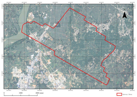
Figure 4.
Orthophoto of the survey area.
The survey area was surveyed in autumn 2018 with a five-camera oblique imaging system mounted on a VTOL (Vertical Take-Off and Landing) fixed-wing UAV, and a total of 9775 images were acquired. Figure 5 illustrates the camera setup of the oblique imaging system. Specifications for the data acquisition are listed in Table 1.
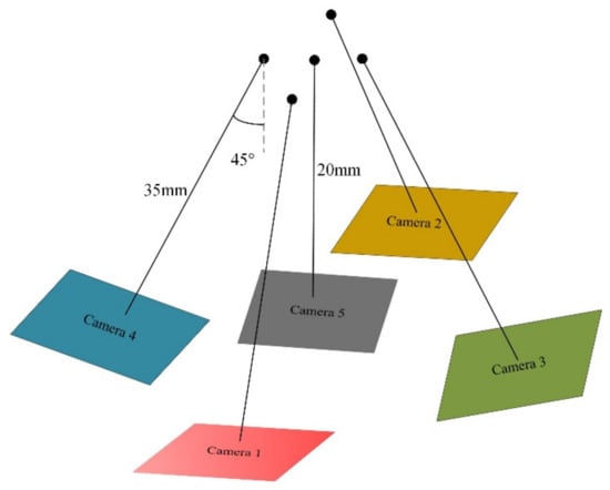
Figure 5.
Setup of cameras.

Table 1.
Specifications for data acquisition.
The acquired POS data include absolute position and orientation observations. The position observations include latitude, longitude and altitude defined under the World Geodetic System 1984 (WGS84). The orientation observations include Omega, Phi and Kappa which define sequential rotations of the imaging system about X-Y-Z axes of the object coordinate system. Figure 6 shows the position of all 1955 exposures in the survey area. At each exposure point, five images were acquired simultaneously.
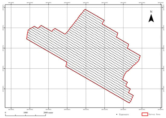
Figure 6.
Position of exposures.
3.2. Model Training and Building Detection in Nadir Images
The satellite datasets used for model training consisted of the open dataset from the crowdAI Mapping Challenge [54] and a dataset manually labelled based on Google satellite imagery of the survey area. The open dataset from the crowdAI Mapping Challenge contained tiles of satellite imagery, along with corresponding annotations. The dataset was split into a training set and a validation set. The training set and validation set contained 280,741 and 60,317 tiles of satellite imagery (as 300 × 300 pixel RGB images), respectively. The corresponding annotations of the training set and validation set were in MS-COCO format [55]. Figure 7 shows sample tiles and annotations from the crowdAI Mapping Challenge.
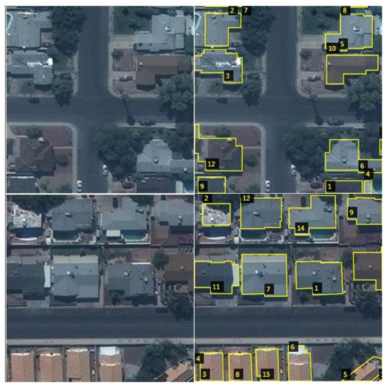
Figure 7.
Sample tiles and annotations from crowdAI Mapping Challenge.
The model training in this work was based on the implementation of [38]. The Mask R-CNN model was trained for 160 epochs on the training set. Firstly, the head of the model was trained for 40 epochs with a 0.001 learning rate. Then, the layers from the fourth to the head were trained for 80 epochs with a 0.001 learning rate. Finally, all of the layers were fine-tuned for 40 epochs with a 0.0001 learning rate. It took about 86 h to complete the 160 epochs of model training. Figure 8 shows the loss on the training set and the validation set during the training process. The loss on the validation set shows that the model begins to overfit after 60 epochs of training. To reduce the influence of the overfitting, an early stopping scheme has been adopted and the model trained for 60 epochs was selected for subsequent training.
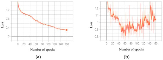
Figure 8.
Loss on: (a) training set; (b) validation set.
Buildings from the crowdAI Mapping Challenge are quite different from those in the survey area. As a consequence, the Mask R-CNN model trained on the crowdAI dataset did not transfer well to UAV images of the survey area. To improve the performance of the model, a dataset of the survey area was manually labelled and used for the subsequent training. A total of 98 image tiles covering typical ground objects including buildings, farmland and vegetation were manually labelled based on Google satellite imagery of the survey area. The tiles were labelled using the VGG Image Annotator (VIA) toolkit [56]. Figure 9 shows sample tiles and corresponding annotations. The model was trained for two epochs on this training set. Firstly, the head of the model was trained for one epoch. Then, the layers from the fourth to the head were trained for another one epoch. The preparation of the satellite dataset of the survey area took less than half an hour and the model training on this dataset took about several minutes.

Figure 9.
Sample tiles and corresponding annotations of the survey area.
The generated model was used to detect buildings in the nadir UAV images. To speed up the building detection process, the nadir images were firstly downsampled to 900 by 600 pixels and then cropped to tiles. The downsampling was conducted using the free and open-source software ImageMagick 7.0.9–25. A total of 11,730 tiles were generated. Figure 10 shows examples of building detection in the tiles. The left column of the figure shows two sample image tiles. The central column shows buildings detected using the model trained only on the crowdAI dataset, and the right column shows buildings detected using the model trained on both the crowdAI dataset and the dataset of the survey area. The detected buildings are indicated with bounding boxes. The confidence score of each detected building is also labelled. It can be seen from the figure that many false positives and false negatives exist in the buildings detected using the model trained only on the crowdAI dataset. The false positives and false negatives are significantly reduced by subsequent training on the dataset of the survey area. It is also worth noting that the confidence scores of the true positives are also increased. The results show that the trained Mask R-CNN model works well in detecting buildings in the nadir images.
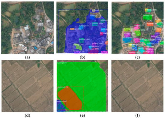
Figure 10.
Examples of building detection: (a) sample image tile1; (b) buildings detected in tile1 using model trained on crowdAI dataset; (c) buildings detected in tile1 using model trained on datasets of crowdAI and survey area; (d) sample image tile2; (e) buildings detected in tile2 using model trained on crowdAI dataset; (f) buildings detected in tile2 using model trained on datasets of crowdAI and survey area.
Although most false positives can be removed by training on the dataset of the survey area, a few still exist in the building detection results. These false positives were removed using the threshold for confidence score. To set the threshold value, the influence of the confidence score on view selection was evaluated using the nadir images. A total of 1290 out of 1955 nadir images were manually classified as building-covering images and used as the ground truth. Figure 11 illustrates the evaluation result. It can be seen that the precision of view selection consistently increases with the confidence score, and it reaches 0.982 when the score is 0.999. The accuracy and F1 score increase with the confidence score until the score reaches 0.999. The recall of the view selection slightly decreases with the confidence score, and it drops to 0.898 when the score reaches 0.999. By investigating the false negatives, it was found that they were mainly images that covered either a single atypical building or only parts of buildings. In consideration of the fact that most buildings were located in several settlements and each building was observable in several neighbouring photos, the threshold for the confidence score was set as 0.999 in this work. A total of 6008 valid building instances were determined using this threshold.
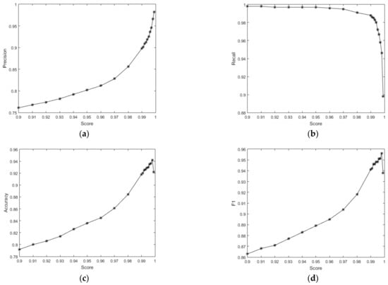
Figure 11.
Influence of score on view selection: (a) precision; (b) recall; (c) accuracy; (d) F1 score.
3.3. Direct Georeferencing of Valid Building Instances and UAV Images
In this work, an ASTER GDEM2 elevation model of the survey area was used for DEM-aided direct georeferencing of the valid building instances and the UAV images. The ASTER GDEM2 elevation model of the survey area was downloaded using the USGS EarthExplorer as a GeoTIFF file. The resolution of the file is 3601 by 3601 pixels, and the spatial resolution is about 30 m. The direct georeferencing result of the 6008 valid building instances and the ground truth are shown in Figure 12a. The ground truth containing 4055 building points labelled manually in the orthomosaic generated from the nadir UAV images is shown in Figure 12b. It can be seen that the directly-georeferenced building points and the ground truth largely overlap with each other. The number of georeferenced building points is higher than that of the ground truth. This is because each building was observable in several neighbouring nadir images. There are several false positives located in the river. These false positives result from boats, which are similar in shape to a building. By comparison of these two figures, it can be found that the number of false negatives is small. The result demonstrates the effectiveness of the building detection and direct georeferencing methods.
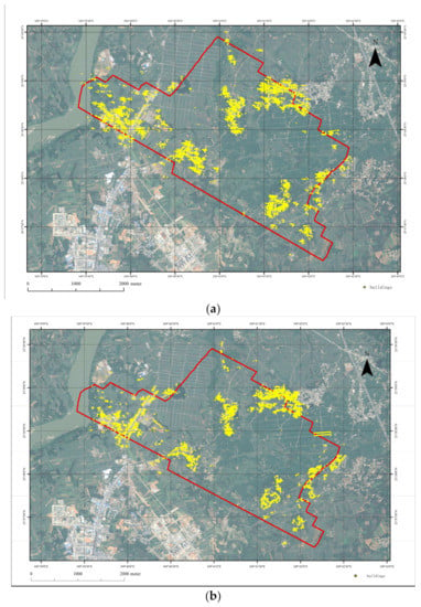
Figure 12.
Building points: (a) direct georeferencing of valid building instances; (b) the ground truth.
The directly-georeferenced principal points of images are shown in Figure 13. Principal points from different cameras are distinguished by color. Figure 13a shows that the principal points belonging to the backward-looking camera, the forward-looking camera and the nadir camera are approximately collinear. Figure 13b shows that the principal points belonging to the right-looking camera and the left-looking camera are approximately located in neighbouring lines. The spatial proximity between the principal points reflects the neighbouring relationship between corresponding images, which visually justifies the proposed match pair selection method.
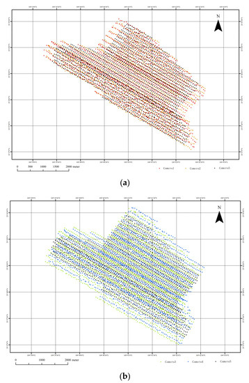
Figure 13.
Directly-georeferenced principal points of UAV images from: (a) Camera 1, 2 and 5; (b) Camera 3, 4 and 5.
3.4. Oblique View Selection and Match Pair Generation
On the basis of georeferencing of the valid building instances and UAV images, building-covering oblique images were selected by nearest neighbours search. The length of the search radius R was set as 140 m which corresponded to half the ground length of the short side of an image. The length of the search radius was calculated using the image resolution and the ground sample distance listed in Table 1. Figure 14 illustrates the view selection of an oblique image. Figure 14a shows an image (no. 415) from Camera 1 (the backward-looking camera). Figure 14b shows the search circle of the image overlaid on the georeferenced building points. The center of the search circle is the georeferenced principal point of the image. The red arrow in Figure 14b shows the flight direction of the UAV. The search circle and the flight direction are also labelled in the image to illustrate the spatial relationship between these two figures. It can be seen that there are many buildings in the aerial image. The buildings are mainly located at the central and bottom parts of the image. Few buildings are located at the top-left and top-right parts of the image. It can be seen from Figure 14b that the distribution of the georeferenced building points is consistent with that in the aerial image, which further demonstrates the correctness of the building detection and direct georeferencing methods. The image was automatically selected as many building points were searched within the circle.
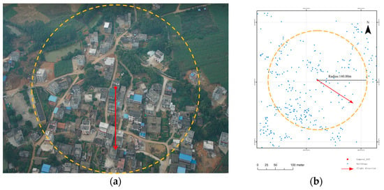
Figure 14.
Illustration of view selection based on nearest neighbours search: (a) an oblique image from Camera 1; (b) the search circle of the image overlaid on the georeferenced building points.
A total of 4441 oblique images were selected by the oblique view selection procedure. To evaluate the result of oblique view selection, the ground truth was prepared manually for images from each oblique camera. The evaluation result is listed in Table 2. It can be seen from the table that the number of selected oblique images is close to the ground truth for each camera. The precision, recall, accuracy and F1 score of view selection for the oblique cameras are close, which shows the versatility of the proposed methodology. The average precision and recall of the view selection are 0.9 and 0.88, respectively. The high F1 score shows a good balance between the precision and recall is achieved.

Table 2.
Evaluation of oblique view selection.
By investigating the false negative images, it is found that buildings are basically located in the corners of these images. It should be noted that most of the buildings in the false negative images are observable in the true positive images, and therefore these buildings can still be reconstructed. Moreover, the spatial resolution of the buildings in the true positive images is higher than that in the false negative ones because of the much shorter observation distance. A careful examination was conducted to find all the missing buildings that could not be reconstructed. A building is considered as missing if the number of observations from any oblique camera is less than two. A total of 23 missing buildings were found. These missing buildings were atypical buildings that were not detected in the nadir images. These buildings were also far from other detected buildings and, therefore, were not covered by the selected oblique images. Except for the missing ones, a total of 4032 buildings were covered by the selected oblique images, which accounted for 99.4% of all the buildings in the survey area. The evaluation result demonstrates the effectiveness of the view selection method.
Match pairs were generated from the selected oblique images and all the nadir images. Parameters for match pair generation were set as follows. The length of radius for overlapping image search was set as 505 m, which corresponded to the largest ground distance between the principal points of two overlapping images. The length of the radius was calculated using the image resolution and the ground sample distance listed in Table 1. Parameters k1, k2, k3 and k4 were set as 2, 2, 1 and 4, respectively. Threshold for viewing direction filtering was set as 50 degrees. A total of 16,261 match pairs were generated. To evaluate the effectiveness of the proposed match pair generation method, the selected oblique images and the nadir images were matched according to the generated match pairs. RootSIFT with the approximate nearest neighbours (ANN) algorithm from the open-source software OpenMVG was used for pairwise image matching [57]. To speed up the matching process, the aforementioned downsampled images were used for the experiments. A total of 15,605 match pairs were robustly matched. The number and percentage of matched image pairs are listed in Table 3. The percentage of matched pairs from each single camera is higher than 99%. The percentage of matched backward-forward and right-left image pairs are 94% and 97.2%, respectively. The percentage of matched oblique-nadir pairs is between 84.0% and 93.8%. The pairwise image matching result shows the effectiveness of the proposed match pair generation method.

Table 3.
Number and percentage of robustly matched image pairs.
3.5. Comparison of Pipelines
The proposed methodology was evaluated for SfM and dense cloud reconstruction. The data processing pipeline based on the proposed methodology was compared with the traditional pipeline from the open-source software OpenMVG [57] for SfM reconstruction. The SfM pipeline from OpenMVG reconstructed a sparse model using all the 9775 images. Firstly, position-based match pair generation was used for match pair generation. The number of nearest neighbours for the position-based match pair generation was set as 100 in the experiments. Secondly, RootSIFT with ANN was used for pair-wise image matching. Finally, an incremental SfM was used for sparse reconstruction based on the robustly matched tie points.
The SfM pipeline based on the proposed methodology reconstructed a sparse model as follows. Firstly, oblique images that cover buildings were selected by the proposed methodology. Then, match pairs were selected using the proposed match pair generation method. Third, RootSIFT with ANN was used for pair-wise image matching. Finally, an incremental SfM was used for sparse reconstruction based on the robustly matched tie points. The SfM reconstruction results were compared in terms of completeness, accuracy, and efficiency. For the evaluation of completeness, the percentage of registered images after SfM reconstruction was compared. For the evaluation of accuracy, RMSE (Root Mean Square Error) of reprojection errors was used as the measure. For the evaluation of efficiency, the time consumed by image matching and SfM reconstruction was compared. To speed up the data processing workflow and comparison without loss of generality, the aforementioned downsampled images were used for the SfM experiments.
Figure 15 shows the sparse models reconstructed by two pipelines. Figure 15a,b are the top and horizontal views of the sparse model reconstructed by the traditional pipeline. Figure 15c,d are the top and horizontal views of the sparse model reconstructed by the proposed pipeline. The green points in the figures show the position of oriented images. The top views show the difference of sparse point clouds reconstructed by the pipelines. The point densities in Figure 15a,c are similar in the building areas and significantly different in other areas. Traditional pipeline reconstructed the scene using all the images without discrimination of ground objects. The pipeline based on the proposed methodology reconstructed the scene using 6396 images (4441 selected oblique images and 1955 nadir images), which resulted in variational point density. The horizontal views show that the oriented images are approximately in a plane, and the reconstructed terrain is approximately flat, which is consistent with the ground truth. However, Figure 15b shows that many outlier points existed in the sparse point cloud generated by the traditional pipeline. These outliers are scattered in the space above and under the ground plane. In contrast, Figure 15d shows that fewer outliers existed in the sparse point cloud generated based on the proposed methodology. The reconstruction of the sparse model demonstrates the adaptiveness and accuracy of the proposed methodology.
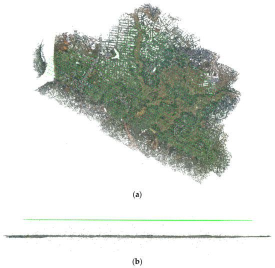
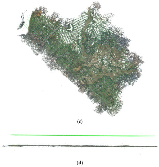
Figure 15.
Sparse models reconstructed by: (a) traditional pipeline (top view); (b) traditional pipeline (horizontal view); (c) proposed pipeline (top view); (d) proposed pipeline (horizontal view).
Statistics of sparse reconstruction based on the traditional pipeline and the proposed pipeline are listed in Table 4.

Table 4.
Statistics of sparse reconstruction based on the traditional pipeline and the proposed pipeline.
- Completeness
It can be seen from Table 4 that both pipelines achieved relatively complete reconstruction. The traditional pipeline registered 99.80% of 9775 images. The proposed pipeline registered 99.83% of 6396 images. The high completeness of the reconstruction shows the precision and robustness of the proposed match pair generation method.
- Accuracy
Both pipelines reported subpixel level of RMSE in SfM reconstruction. The traditional pipeline achieved 0.49 pixels of RMSE. The proposed pipeline achieved 0.42 pixels of RMSE, which is smaller than that of the traditional pipeline. The evaluation results show the high accuracy of the proposed methodology.
- Efficiency
Table 4 shows the time efficiency of the pipelines. It took the traditional pipeline more than 22 h to complete the processing, whereas the proposed pipeline completed the processing within 7 h. Specifically, the proposed pipeline spent 0.5 h, 1 h, 2.5 s, 11 min and 5 h and 15 min on data preparation and model training, oblique view selection, match pair generation, image matching and SfM reconstruction, respectively. It is worth mentioning that the data preparation and model training in Table 4 refers to the preparation of the satellite dataset of the survey area and the training on this dataset. The time taken for model training on the crowdAI dataset is not included, as a model is trained only once on this dataset, and the trained model is reused as a pre-trained model to be fine-tuned on a dataset of a specific area. The comparison results show that the proposed pipeline reduced 68.9% of the data processing time.
Dense clouds of the area shown in Figure 14 were generated, respectively, based on the sparse reconstructions by two pipelines using the open-source software OpenMVS [58]. Additionally, the points of four typical buildings were randomly selected from the dense clouds and used for comparison. The selected buildings are illustrated by Figure 16.
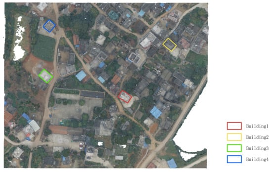
Figure 16.
Buildings selected for dense cloud comparison.
For each building, distances between dense points generated based on two pipelines were computed using the M3C2 distance plugin (Multiscale Model to Model Cloud Comparison) [59] available in the open-source software CloudCompare [60]. Two point clouds of each building were aligned using the Iterative Closest Point (ICP) algorithm [61], based on 50,000 random sample points, before the computation of points to points distances (PTPD). Statistics of PTPD of the four selected buildings are listed in Table 5. The maximum PTPD values of Building 1, 2 and 4 are less than one meter, and the maximum PTPD value of Building 3 is slightly larger than one meter. The average PTPD values of all four buildings are 5 or 6 cm, and the standard deviations of PTPD values of the four buildings are 3 or 4 cm, which are equivalent to 0.43 or 0.57 of GSD.

Table 5.
Statistics of distances between dense points generated based on the traditional pipeline and the proposed pipeline.
Figure 17 visualizes colourized point clouds and the corresponding PTPD values of each building. The left column shows the point clouds of the buildings generated based on the proposed pipeline. The right column visualizes the PTPD values for each building. The legend of the figures in the right column shows the spatial and range distribution of the PTPD values. It can be seen from the figure that the majority of the PTPD values of each building are in the range of several centimeters. Large PTPD values are basically located at highly occluded points or points of windows. Dense matching of these points is highly uncertain due to unsatisfactory observing conditions. The statistics and visualization of the PTPD values show high consistency between the point clouds of buildings reconstructed using all the images based on the traditional pipeline and the selected images based on the proposed pipeline.
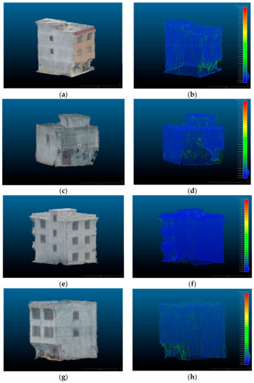
Figure 17.
Point clouds and corresponding PTPD values: (a) point cloud of Building 1; (b) PTPD values of Building 1; (c) point cloud of Building 2; (d) PTPD values of Building 2; (e) point cloud of Building 3; (f) PTPD values of Building 3; (g) point cloud of Building 4; (h) PTPD values of Building 4.
4. Discussion
The proposed methodology utilizes semantic information to select the images covering buildings and generate match pairs for the selected images. Experiments show significant improvement in efficiency by incorporating the proposed methodology in the classical SfM pipeline.
The accuracy of a sparse reconstruction reflects the inner consistency of a model. A sparse reconstruction is optimized by Bundle block adjustment (BBA) based on tie point observations. More images lead to more tie point observations and a more stable block structure. If all tie point observations are of the same accuracy, more observations generally lead to more accurate SfM reconstruction and smaller RMSE of reprojection errors. However, the experimental results have shown that the accuracy of the sparse reconstruction using the entire image set is not higher than that using the semantically selected images. The main reason is that the accuracies of tie point observations are not the same. Images with repetitive textures (e.g., farmland) are prone to outliers, and outliers undermine the overall accuracy of BBA of the entire image set. By semantically selecting images covering buildings, the proposed pipeline objectively excludes many images with repetitive textures from the spare reconstruction and reduces outliers (Figure 15). The experimental results show that fewer but better tie point observations still guarantee the accuracy of a sparse reconstruction.
The improvement in efficiency benefits from oblique view selection and match pair generation. As stated above, the proposed pipeline excludes many images with repetitive textures from sparse reconstruction, which reduces the number of images to process. Match pair generation is also crucial for the efficiency and robustness of SfM reconstruction. The position-based match pair generation method used by OpenMVG selects match pairs using spatial distance between images, but neighbouring oblique images do not necessarily overlap, and pairwise image matching based on these false match pairs is prone to false tie points. The proposed methodology selects match pairs by using direct georeferencing, which takes into account the position of images, viewing directions of images and the terrain of a survey area. Additionally, the number of generated match pairs is constrained to control the redundancy of the match graph. The proposed methodology generates fewer but more precise match pairs. Therefore, SfM reconstruction based on the proposed match pair generation method is more efficient.
The accuracy and completeness of the dense reconstruction is guaranteed by the accurate and robust sparse reconstruction based on the proposed pipeline. The comparison of dense clouds shows high consistency between the dense reconstructions of buildings based on the proposed pipeline and the traditional pipeline. Accurate sparse reconstruction generally leads to accurate dense reconstruction. Therefore, the accuracy of the dense cloud generated based on the proposed pipeline is comparable to that based on the traditional pipeline. Moreover, as almost all images that cover buildings have been selected and used for dense reconstruction, the completeness of dense reconstruction of buildings is also guaranteed.
The experimental results demonstrate that semantics-aided 3D reconstruction is much more efficient than the traditional pipeline, and it is still accurate and complete. Therefore, it can be used in regular data production work as well as time-critical applications such as disaster management and emergency response. For example, to evaluate the impact of an earthquake on residential houses and civil infrastructures in an area, the images that cover houses and civil infrastructures can be selected and used for efficient 3D reconstruction. Based on 3D reconstruction and semantic information, object level change detection and destruction evaluation can be obtained.
5. Conclusions
An oblique view selection methodology for efficient and accurate building reconstruction in rural areas is proposed in this paper. The proposed methodology effectively selects oblique images that cover buildings in a survey area based on instance segmentation and direct georeferencing. Match pairs are generated based on nearest neighbours search for matching the nadir images and the selected oblique images. The proposed methodology was tested on a dataset containing 9775 UAV images. A total of 4441 oblique images covering 99.4% of all the buildings in the survey area were automatically selected. The average precision and recall of the oblique view selection are 0.90 and 0.88, respectively. The percentage of robustly matched oblique-oblique and oblique-nadir image pairs are above 94% and 84.0%, respectively. The sparse reconstruction based on the proposed methodology significantly outperforms that based on the traditional pipeline in terms of efficiency, and it is comparably accurate and complete. The comparison of dense point clouds shows high consistency between buildings reconstructed using all the images based on the traditional pipeline and the selected images based on the proposed pipeline.
The effectiveness of the proposed methodology shows the benefits of semantic information for large-scale UAV photogrammetry. As the means and frequency of earth observations increase, more and more high quality datasets for ground object segmentation become available. At the same time, with the continuous advancement of pattern recognition and machine learning techniques, semantics-aided 3D reconstruction will be widely used.
Author Contributions
Conceptualization, Y.L.; methodology, Y.L.; software, Y.L.; validation, Y.L., X.F. and Y.Y.; formal analysis, Y.L.; investigation, Y.L.; resources, T.C.; data curation, Y.L.; writing—original draft preparation, Y.L.; writing—review and editing, Y.L.; visualization, Y.L., X.F., Y.Y. and D.L.; project administration, Y.L.; funding acquisition, T.C. All authors have read and agreed to the published version of the manuscript.
Funding
This research was funded by the Special Foundation for National Science and Technology Basic Research Program of China, grant number 2019FY202500.
Informed Consent Statement
Not applicable.
Data Availability Statement
The data presented in this study are available on request from the corresponding author.
Conflicts of Interest
The authors declare no conflict of interest.
References
- Batty, M. Model Cities. Town Planning Rev. 2007, 78, 125–151. [Google Scholar] [CrossRef]
- Gröger, G.; Plümer, L. CityGML—Interoperable semantic 3D city models. ISPRS J. Photogramm. Remote Sens. 2012, 71, 12–33. [Google Scholar] [CrossRef]
- Ham, Y.; Han, K.K.; Lin, J.J.; Golparvar-Fard, M. Visual monitoring of civil infrastructure systems via camera-equipped Unmanned Aerial Vehicles (UAVs): A review of related works. Vis. Eng. 2016, 4, 1. [Google Scholar] [CrossRef] [Green Version]
- Duarte, D.; Nex, F.; Kerle, N.; Vosselman, G. Detection of seismic façade damages with multi-temporal oblique aerial imagery. GISci. Remote Sens. 2020, 57, 670–686. [Google Scholar] [CrossRef]
- Gerke, M.; Kerle, N. Automatic structural seismic damage assessment with airborne oblique Pictometry© imagery. Photogramm. Eng. Remote Sens. 2011, 77, 885–898. [Google Scholar] [CrossRef]
- Giordan, D.; Hayakawa, Y.; Nex, F.; Remondino, F.; Tarolli, P. Review article: The use of remotely piloted aircraft systems (RPASs) for natural hazards monitoring and management. Nat. Hazards Earth Syst. Sci. 2018, 18, 1079–1096. [Google Scholar] [CrossRef] [Green Version]
- Vetrivel, A.; Gerke, M.; Kerle, N.; Nex, F.; Vosselman, G. Disaster damage detection through synergistic use of deep learning and 3D point cloud features derived from very high resolution oblique aerial images, and multiple-kernel-learning. ISPRS J. Photogramm. Remote Sens. 2018, 140, 45–59. [Google Scholar] [CrossRef]
- Fernández-Hernandez, J.; González-Aguilera, D.; Rodríguez-Gonzálvez, P.; Mancera-Taboada, J. Image-based modelling from unmanned aerial vehicle (uav) photogrammetry: An effective, low-cost tool for archaeological applications. Archaeometry 2015, 57, 128–145. [Google Scholar] [CrossRef]
- Colomina, I.; Molina, P. Unmanned aerial systems for photogrammetry and remote sensing: A review. ISPRS J. Photogramm. Remote Sens. 2014, 92, 79–97. [Google Scholar] [CrossRef] [Green Version]
- Haala, N.; Kada, M. An update on automatic 3D building reconstruction. ISPRS J. Photogramm. Remote Sens. 2010, 65, 570–580. [Google Scholar] [CrossRef]
- Nex, F.; Remondino, F. UAV for 3D mapping applications: A review. Appl. Geomat. 2014, 6, 1–15. [Google Scholar] [CrossRef]
- Pajares, G. Overview and current status of remote sensing applications based on unmanned aerial vehicles (UAVs). Photogramm. Eng. Remote Sens. 2015, 81, 281–330. [Google Scholar] [CrossRef] [Green Version]
- Remondino, F.; Barazzetti, L.; Nex, F.; Scaioni, M.; Sarazzi, D. UAV photogrammetry for mapping and 3d modeling–current status and future perspectives. Int. Arch. Photogramm. Remote Sens. Spat. Inf. Sci. 2011, 38, C22. [Google Scholar] [CrossRef] [Green Version]
- Lowe, D.G. Distinctive Image features from scale-invariant keypoints. Int. J. Comput. Vis. 2004, 60, 91–110. [Google Scholar] [CrossRef]
- Arya, S.; Mount, D.M.; Netanyahu, N.S.; Silverman, R.; Wu, A.Y. An optimal algorithm for approximate nearest neighbor searching fixed dimensions. J. ACM 1998, 45, 891–923. [Google Scholar] [CrossRef] [Green Version]
- Muja, M.; Lowe, D.G. Scalable nearest neighbor algorithms for high dimensional data. IEEE Trans. Pattern Anal. Mach. Intell. 2014, 36, 2227–2240. [Google Scholar] [CrossRef]
- Hartley, R.; Zisserman, A. Multiple View Geometry in Computer Vision, 2nd ed.; Cambridge University Press: Cambridge, UK, 2004. [Google Scholar]
- Snavely, N.; Seitz, S.M.; Szeliski, R. Photo tourism: Exploring photo collections in 3D. ACM Trans. Graph. 2006, 25, 835–846. [Google Scholar] [CrossRef]
- Agarwal, S.; Furukawa, Y.; Snavely, N.; Simon, I.; Curless, B.; Seitz, S.M.; Szeliski, R. Building Rome in a Day. Commun. ACM 2011, 54, 105–112. [Google Scholar] [CrossRef]
- Snavely, N.; Seitz, S.M.; Szeliski, R. Modeling the world from internet photo collections. Int. J. Comput. Vis. 2008, 80, 189–210. [Google Scholar] [CrossRef] [Green Version]
- Schönberger, J.L.; Frahm, J.-M. Structure-from-motion revisited. In Proceedings of the IEEE Conference on Computer Vision and Pattern Recognition, Las Vegas, NV, USA, 27–30 June 2016; pp. 4104–4113. [Google Scholar]
- Gerke, M.; Nex, F.; Remondino, F.; Jacobsen, K.; Kremer, J.; Karel, W.; Hu, H.; Ostrowski, W. Orientation of oblique airborne image sets—Experiences from the ISPRS/EUROSDR benchmark on multi-platform photogrammetry. Int. Arch. Photogramm. Remote Sens. Spat. Inf. Sci. 2016, XLI-B1, 185–191. [Google Scholar] [CrossRef] [Green Version]
- Jiang, S.; Jiang, C.; Jiang, W. Efficient structure from motion for large-scale UAV images: A review and a comparison of SfM tools. ISPRS J. Photogramm. Remote Sens. 2020, 167, 230–251. [Google Scholar] [CrossRef]
- Hirschmüller, H. Stereo Processing by Semiglobal Matching and Mutual Information. IEEE Trans. Pattern Anal. Mach. Intell. 2008, 30, 328–341. [Google Scholar] [CrossRef] [PubMed]
- Furukawa, Y.; Ponce, J. Accurate, dense, and robust multiview stereopsis. IEEE Trans. Pattern Anal. Mach. Intell. 2010, 32, 1362–1376. [Google Scholar] [CrossRef]
- Schönberger, J.L.; Zheng, E.; Frahm, J.-M.; Pollefeys, M. Pixelwise view selection for unstructured multi-view stereo. In Proceedings of the European Conference on Computer Vision, Amsterdam, The Netherlands, 8–16 October 2016; pp. 501–518. [Google Scholar]
- Kazhdan, M.; Bolitho, M.; Hoppe, H. Poisson surface reconstruction. In Proceedings of the Fourth Eurographics Symposium on Geometry Processing, Cagliari Sardinia, Italy, 26–28 June 2006. [Google Scholar]
- Hasheminasab, S.M.; Zhou, T.; Habib, A. GNSS/INS-Assisted structure from motion strategies for UAV-Based imagery over mechanized agricultural fields. Remote Sens. 2020, 12, 351. [Google Scholar] [CrossRef] [Green Version]
- Zhang, L.; Du, B. Deep Learning for Remote Sensing Data: A Technical Tutorial on the State of the Art. IEEE Geosci. Remote Sens. Mag. 2016, 4, 22–40. [Google Scholar] [CrossRef]
- Zhu, X.X.; Tuia, D.; Mou, L.; Xia, G.; Zhang, L.; Xu, F.; Fraundorfer, F. Deep Learning in Remote Sensing: A Comprehensive Review and List of Resources. IEEE Geosci. Remote Sens. Mag. 2017, 5, 8–36. [Google Scholar] [CrossRef] [Green Version]
- Ma, L.; Liu, Y.; Zhang, X.; Ye, Y.; Yin, G.; Johnson, B.A. Deep learning in remote sensing applications: A meta-analysis and review. ISPRS J. Photogramm. Remote Sens. 2019, 152, 166–177. [Google Scholar] [CrossRef]
- Wu, G.; Shao, X.; Guo, Z.; Chen, Q.; Yuan, W.; Shi, X.; Xu, Y.; Shibasaki, R. Automatic building segmentation of aerial imagery using multi-constraint fully convolutional networks. Remote Sens. 2018, 10, 407. [Google Scholar] [CrossRef] [Green Version]
- Ji, S.; Wei, S.; Lu, M. Fully Convolutional Networks for Multisource Building Extraction From an Open Aerial and Satellite Imagery Data Set. IEEE Trans. Geosci. Remote Sens. 2019, 57, 574–586. [Google Scholar] [CrossRef]
- Yi, Y.; Zhang, Z.; Zhang, W.; Zhang, C.; Li, W.; Zhao, T. Semantic Segmentation of Urban Buildings from VHR Remote Sensing Imagery Using a Deep Convolutional Neural Network. Remote Sens. 2019, 11, 1774. [Google Scholar] [CrossRef] [Green Version]
- Zhuo, X.; Fraundorfer, F.; Kurz, F.; Reinartz, P. Optimization of OpenStreetMap Building Footprints Based on Semantic Information of Oblique UAV Images. Remote Sens. 2018, 10, 624. [Google Scholar] [CrossRef] [Green Version]
- Li, W.; He, C.; Fang, J.; Zheng, J.; Fu, H.; Yu, L. Semantic segmentation-based building footprint extraction using very high-resolution satellite images and multi-source GIS data. Remote Sens. 2019, 11, 403. [Google Scholar] [CrossRef] [Green Version]
- Zhao, W.; Persello, C.; Stein, A. Building outline delineation: From aerial images to polygons with an improved end-to-end learning framework. ISPRS J. Photogramm. Remote Sens. 2021, 175, 119–131. [Google Scholar] [CrossRef]
- Mohanty, S.P.; Czakon, J.; Kaczmarek, K.A.; Pyskir, A.; Tarasiewicz, P.; Kunwar, S.; Rohrbach, J.; Luo, D.; Prasad, M.; Fleer, S.; et al. Deep Learning for Understanding Satellite Imagery: An Experimental Survey. Front Artif. Intell. 2020, 3, 534696. [Google Scholar] [CrossRef] [PubMed]
- Chen, J.; Wang, G.; Luo, L.; Gong, W.; Cheng, Z. Building Area Estimation in Drone Aerial Images Based on Mask R-CNN. IEEE Geosci. Remote. Sens. Lett. 2021, 18, 891–894. [Google Scholar] [CrossRef]
- Gevaert, C.M.; Persello, C.; Sliuzas, R.; Vosselman, G. Monitoring household upgrading in unplanned settlements with unmanned aerial vehicles. Int. J. Appl. Earth Obs. Geoinf. 2020, 90, 102117. [Google Scholar] [CrossRef]
- Li, Y.; Xu, W.; Chen, H.; Jiang, J.; Li, X. A Novel Framework Based on Mask R-CNN and Histogram Thresholding for Scalable Segmentation of New and Old Rural Buildings. Remote Sens. 2021, 13, 1070. [Google Scholar] [CrossRef]
- Heipke, C.; Rottensteiner, F. Deep learning for geometric and semantic tasks in photogrammetry and remote sensing. Geo-Spat. Inf. Sci. 2020, 23, 10–19. [Google Scholar] [CrossRef]
- Qin, R.; Gruen, A. The role of machine intelligence in photogrammetric 3D modeling—An overview and perspectives. Int. J. Digit. Earth 2020, 14, 15–31. [Google Scholar] [CrossRef]
- Shan, J.; Hu, Z.; Tao, P.; Wang, L.; Zhang, S.; Ji, S. Toward a unified theoretical framework for photogrammetry. Geo-Spat. Inf. Sci. 2020, 23, 75–86. [Google Scholar] [CrossRef]
- Nex, F.; Armenakis, C.; Cramer, M.; Cucci, D.A.; Gerke, M.; Honkavaara, E.; Kukko, A.; Persello, C.; Skaloud, J. UAV in the advent of the twenties: Where we stand and what is next. ISPRS J. Photogramm. Remote Sens. 2022, 184, 215–242. [Google Scholar] [CrossRef]
- Stathopoulou, E.; Remondino, F. Semantic photogrammetry: Boosting image-based 3D reconstruction with semantic labeling. Int. Arch. Photogramm. Remote Sens. Spat. Inf. Sci. 2019, XLII-2/W9, 685–690. [Google Scholar] [CrossRef] [Green Version]
- Stathopoulou, E.K.; Battisti, R.; Cernea, D.; Remondino, F.; Georgopoulos, A. Semantically Derived Geometric Constraints for MVS Reconstruction of Textureless Areas. Remote Sens. 2021, 13, 1053. [Google Scholar] [CrossRef]
- Zhou, G.; Bao, X.; Ye, S.; Wang, H.; Yan, H. Selection of Optimal Building Facade Texture Images From UAV-Based Multiple Oblique Image Flows. IEEE Trans. Geosci. Remote Sens. 2021, 59, 1534–1552. [Google Scholar] [CrossRef]
- Yu, D.; Ji, S.; Liu, J.; Wei, S. Automatic 3D building reconstruction from multi-view aerial images with deep learning. ISPRS J. Photogramm. Remote Sens. 2021, 171, 155–170. [Google Scholar] [CrossRef]
- Yang, C.; Zhang, F.; Gao, Y.; Mao, Z.; Li, L.; Huang, X. Moving Car Recognition and Removal for 3D Urban Modelling Using Oblique Images. Remote Sens. 2021, 13, 3458. [Google Scholar] [CrossRef]
- Oniga, V.-E.; Breaban, A.-I.; Pfeifer, N.; Diac, M. 3D Modeling of Urban Area Based on Oblique UAS Images—An End-to-End Pipeline. Remote Sens. 2022, 14, 422. [Google Scholar] [CrossRef]
- Liang, Y.; Li, D.; Feng, C.; Mao, J.; Wang, Q.; Cui, T. Efficient match pair selection for matching large-scale oblique UAV images using spatial priors. Int. J. Remote Sens. 2021, 42, 8878–8905. [Google Scholar] [CrossRef]
- Bäumker, M.; Heimes, F. New calibration and computing method for direct georeferencing of image and scanner data using the position and angular data of an hybrid inertial navigation system. In Proceedings of the OEEPE Workshop on Integrated Sensor Orientation, Hannover, Germany, 17–18 September 2001; pp. 1–16. [Google Scholar]
- CrowdAI Mapping Challenge Official Web Site. Available online: https://www.aicrowd.com/challenges/mapping-challenge (accessed on 10 January 2022).
- Lin, T.-Y.; Maire, M.; Belongie, S.; Hays, J.; Perona, P.; Ramanan, D.; Dollár, P.; Zitnick, C.L. Microsoft coco: Common objects in context. In Proceedings of the European Conference on Computer Vision, Zurich, Switzerland, 6–12 September 2014; pp. 740–755. [Google Scholar]
- Dutta, A.; Zisserman, A. The VIA annotation software for images, audio and video. In Proceedings of the 27th ACM International Conference on Multimedia, Nice, France, 21–25 October 2019; pp. 2276–2279. [Google Scholar]
- Moulon, P.; Monasse, P.; Perrot, R.; Marlet, R. OpenMVG: Open Multiple View Geometry. In Proceedings of the International Workshop on Reproducible Research in Pattern Recognition, Cancún, Mexico, 4 December 2016; pp. 60–74. [Google Scholar]
- OpenMVS Official Web Site. Available online: https://github.com/cdcseacave/openMVS (accessed on 7 June 2022).
- Lague, D.; Brodu, N.; Leroux, J. Accurate 3D Comparison of Complex Topography with Terrestrial Laser Scanner: Application to the Rangitikei Canyon (NZ). ISPRS J. Photogramm. Remote Sens. 2013, 82, 10–26. [Google Scholar] [CrossRef] [Green Version]
- CloudCompare Official Web Site. Available online: https://www.danielgm.net/cc/ (accessed on 10 June 2022).
- Fischler, M.A.; Bolles, R.C. Random Sample Consensus: A Paradigm for Model Fitting with Applications to Image Analysis and Automated Cartography. Commun. ACM 1981, 24, 381–395. [Google Scholar] [CrossRef]
Publisher’s Note: MDPI stays neutral with regard to jurisdictional claims in published maps and institutional affiliations. |
© 2022 by the authors. Licensee MDPI, Basel, Switzerland. This article is an open access article distributed under the terms and conditions of the Creative Commons Attribution (CC BY) license (https://creativecommons.org/licenses/by/4.0/).