Illumination Geometry and Flying Height Influence Surface Reflectance and NDVI Derived from Multispectral UAS Imagery

Abstract

Small unmanned aerial systems (UAS) have allowed the mapping of vegetation at very high spatial resolution, but a lack of standardisation has led to uncertainties regarding data quality. For reflectance measurements and vegetation indices (Vis) to be comparable between sites and over time, careful flight planning and robust radiometric calibration procedures are required. Two sources of uncertainty that have received little attention until recently are illumination geometry and the effect of flying height. This study developed methods to quantify and visualise these effects in imagery from the Parrot Sequoia, a UAV-mounted multispectral sensor. Change in illumination geometry over one day (14 May 2018) had visible effects on both individual images and orthomosaics. Average near-infrared (NIR) reflectance and NDVI in regions of interest were slightly lower around solar noon, and the contrast between shadowed and well-illuminated areas increased over the day in all multispectral bands. Per-pixel differences in NDVI maps were spatially variable, and much larger than average differences in some areas. Results relating to flying height were inconclusive, though small increases in NIR reflectance with height were observed over a black sailcloth tarp. These results underline the need to consider illumination geometry when carrying out UAS vegetation surveys.

1. Introduction

1.1. Vegetation Mapping with Unmanned Aerial Vehicles

Vegetation mapping using small unmanned aerial systems (UAS) has recently found many applications in environmental and ecological monitoring [1,2,3], forestry [4,5], precision agriculture [6,7] and archaeology [8]. The main advantages of UAS over other remote sensing platforms are the ability to collect data at very high spatial resolution, and a relative ease of deployment, allowing the user to define revisit times appropriate to the phenomena being investigated [1,3]. However, there is a considerable diversity of platforms, sensors and data collection methods [6,9,10], leading to uncertainties regarding data quality. In particular, the influences of collection method and environmental conditions on data quality are poorly understood [9,11]. This creates problems if data from different sources are to be combined, or if time series of observations are to be assembled, as data collected using different sensors and methods or under different environmental conditions may not be comparable.

1.2. From Imagery to Reflectance Measurements

The most common products of multispectral UAS vegetation surveys are orthorectified maps (orthomosaics) of surface reflectance or vegetation indices (VIs) such as the normalised difference vegetation index (NDVI). The sensor does not measure reflectance directly: rather, the digital number (DN) recorded at each pixel must be converted to surface reflectance in two stages: sensor correction and radiometric calibration [10,12,13]. Sensor correction reduces modifications to radiance measurements made by the sensor, including noise, vignetting, lens distortion and spectral variations in sensor response. Kelcey and Lucieer applied corrections for these modifications to data from a six-band multispectral sensor [12], and other researchers have described them for commercial off-the-shelf digital cameras [14,15,16]. Radiometric calibration is the process of retrieving surface reflectance from the corrected image DNs. In principle, this corrects for the effects of environmental conditions such as changing illumination and interactions with the atmosphere [12,13], but is subject to errors caused by non-uniform scene illumination and anisotropic reflectance of vegetation surfaces [17].

1.3. Problems in Radiometric Calibration

The most common approach to radiometric calibration is the empirical line method. Typically, this uses two or more targets with known, stable reflectance to establish a linear relationship between radiance and reflectance [17]. Variants using only one target have also been proposed [18].

The empirical line method has the advantage of simplicity, but makes several assumptions that may not be justified. The relationship between radiance and reflectance is assumed to be linear, and uniform across an image. However, illumination may not be uniform because of shadows cast by clouds or variations in topography, and atmospheric effects can be highly variable even over short distances. Natural surfaces also demonstrate anisotropic reflectance (i.e., they do not reflect equally in all directions), so reflectance measurements are likely to be affected by viewing and illumination geometry [10,17,19].

Newer UAV-mounted multispectral sensors such as the Parrot Sequoia (Parrot Drones SAS, Paris, France) incorporate an ambient light sensor and are calibrated slightly differently—measurements from the multispectral and ambient light sensors are converted to at-sensor radiances in arbitrary units, and a single image of a target with known reflectance is used to calibrate the relationship between the radiances measured at the two sensors [20,21]. This does not resolve the problems with the empirical line method—the ambient light sensor only records one measurement per image, which assumes uniform illumination, while the sensor is typically calibrated on the ground, which ignores any effect of flying height and may introduce errors due to the obstruction of the hemisphere by the UAS or person handling it [19].

Variation in illumination due to cloud shadows can be minimised by avoiding days with scattered clouds [13], but the effects of flying height and of viewing and illumination geometry on UAS imagery are not very well understood, so it is not clear how greatly they affect data quality or how they might be mitigated.

1.4. Effects of Illumination Geometry

Illumination and viewing geometry can be described by the zenith and azimuth angles of the Sun and the sensor at a given pixel, while the angular variation in reflectance of a surface is described by its bidirectional reflectance distribution function (BRDF). Interactions between these cause variations in apparent reflectance across an image. An example that is common in vegetated surfaces is the “hot spot”—a small region of increased brightness seen where the viewing and illumination angles are the same. Here, the sensor views only the illuminated part of the target, so its apparent reflectance is increased compared with regions of the image where there are more shadows [22,23].

Some authors have proposed correction methods for anisotropic reflectance effects in UAS images [10,16,22], and others have used UAS to measure the reflectance anisotropy of surfaces [24,25,26,27,28]. Very few studies have specifically investigated the impact of these effects on data quality in UAS imagery. Rasmussen et al. found significant differences in VIs between image sections in the direction of the Sun and those opposite the Sun, for images captured in sunny conditions [29]. Aasen and Bolten found that the influence of anisotropic reflectance effects differed depending on how the data were processed [19]. They created hyperspectral digital surface models (HS DSMs) using two different processing modes: one where each pixel’s spectral information is an average calculated from the images in which it appears, and another where the spectral information is taken from the image where the pixel is closest to the centre. Anisotropic reflectance effects were visible in the HS DSMs produced without averaging, but appeared to be normalised to some extent when averaging was used.

Solar elevation has also been found to influence VIs in UAS images. Brede et al. found that the enhanced vegetation index (EVI) of a tropical rainforest decreased with increasing solar zenith angle, but NDVI showed a weaker response in the opposite direction, decreasing with increased solar elevation [30]. By contrast, NDVI generally increased with solar elevation at a site in the Canadian Arctic [13], suggesting that the response of VIs to solar elevation may be site-specific.

1.5. Flying Height

Flying height affects both the depth of atmosphere between sensor and target and the spatial resolution of images, but its effect on UAS reflectance measurements has not been investigated in detail [10], possibly because of the small range of flying heights (<120 m) typically used. Yu et al. found that an algorithm to correct for atmospheric path radiance improved the correlation with ground measurements for the normalised excess green index (ExG), and the normalised green-red difference index (NGRDI), especially for greater flying heights (<100 m) [31]. They found no improvement for NDVI, because the effect of path radiance in their model was negligible for red and infrared wavelengths. Rasmussen et al. found no effect of flying height (<100 m) for any of these indices [29].

1.6. Objectives and Research Questions

The objective of this research was to quantify and visualise the effects of illumination geometry and flying height in UAS imagery captured by a Parrot Sequoia sensor. The following research questions were investigated:

• How sensitive to changing solar elevation and azimuth are reflectance and NDVI measured by the Sequoia in individual images and orthomosaics?
• Does flying height influence surface reflectance in Sequoia images and orthomosaics?
• How consistent is reflectance measured by the Sequoia with ground measurements from a field spectrometer?

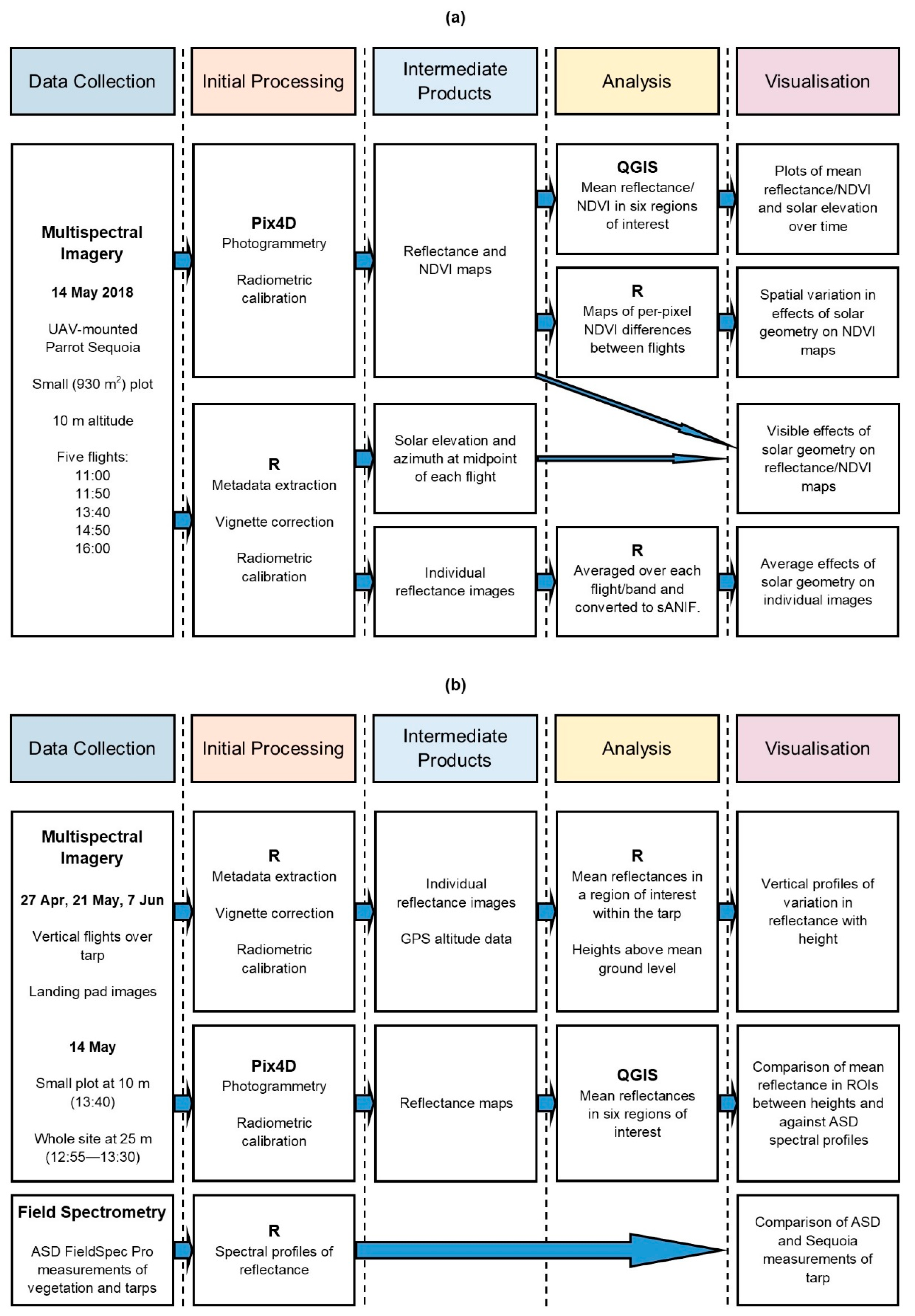
2. Materials and Methods

The workflows used to analyse the effects of illumination geometry and flying height, and for comparing UAS and ground reference data, are summarised in Figure 1. The effects of illumination geometry were assessed using data from five flights over a small (~930 m²) plot, on 14 May 2018. Images were processed in R to obtain individual reflectance images, and in Pix4D to create orthomosaics of reflectance and NDVI. These data were used to analyse and visualise the effect of illumination geometry on individual images and orthomosaics (Figure 1a).

The influence of flying height on individual images was assessed in individual images from vertical flights over a large black tarp on 27 April, 21 May and 7 June 2018. Orthomosaics created from images captured from two different flying heights on 14 May 2018 were also compared. Finally, the UAS data were compared with field spectrometer measurements of the vegetation and tarp collected on all four days (Figure 1b).

2.1. Data Collection

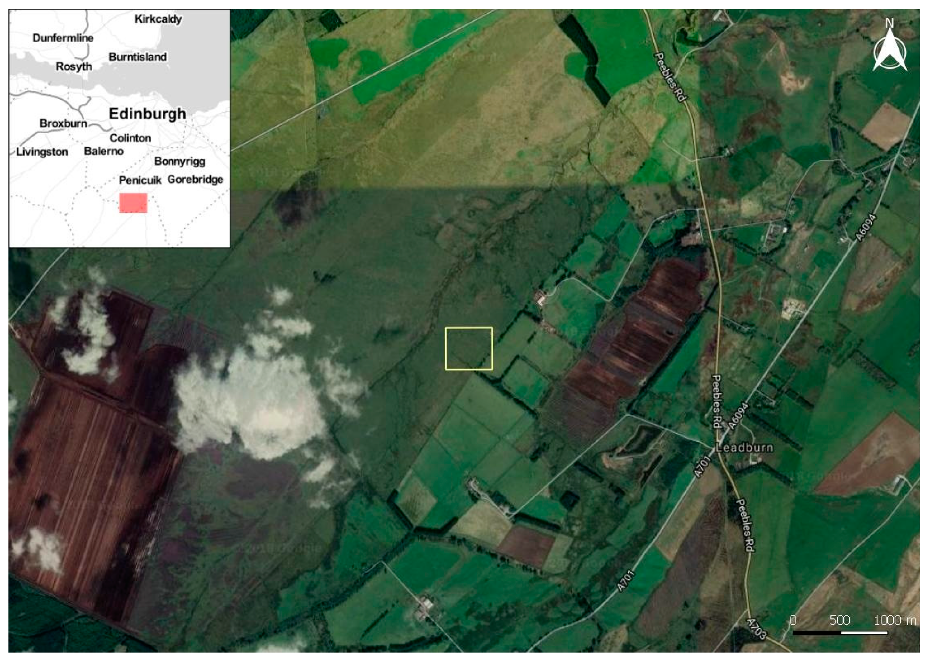
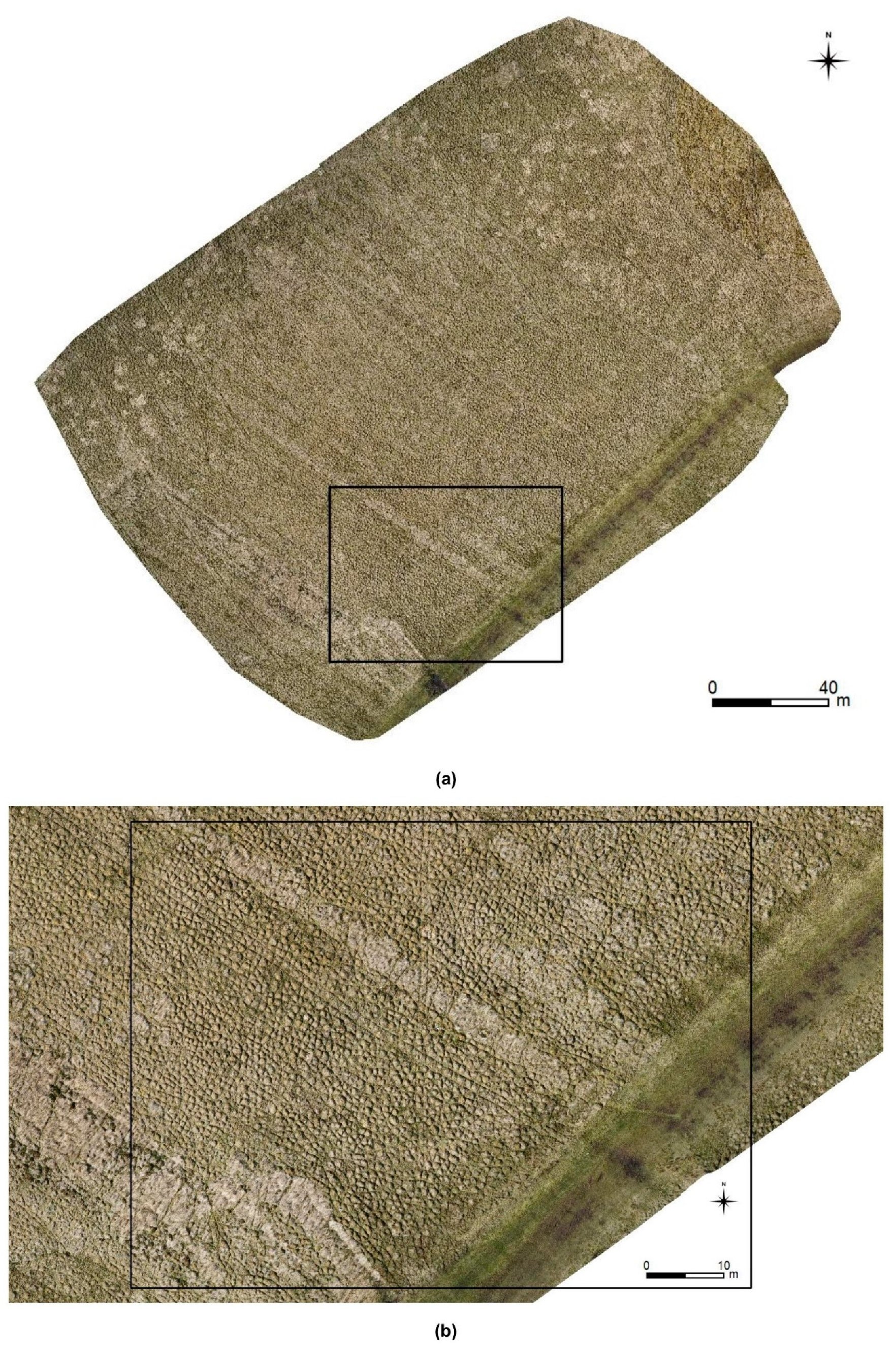
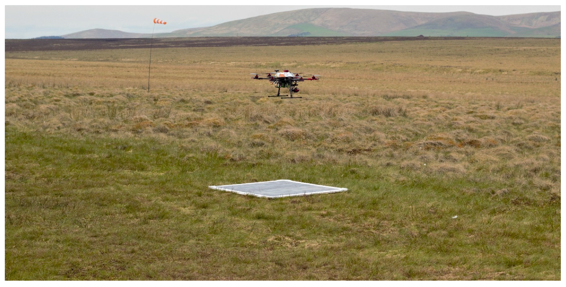
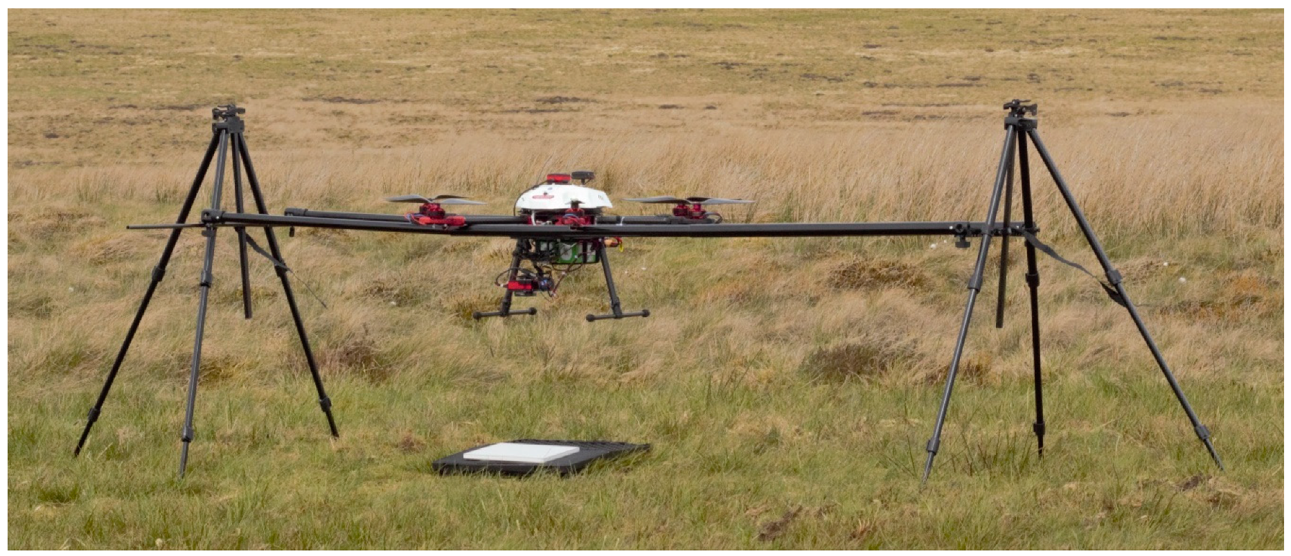
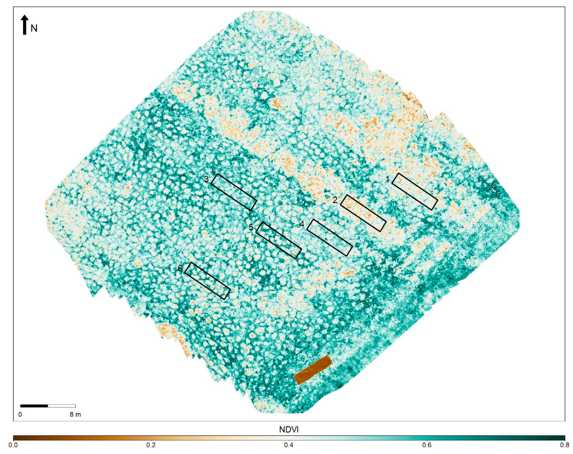
2.1.1. Study Site

All data were collected at Auchencorth Moss (Figure 2), an atmospheric monitoring site in south-central Scotland (55°47’36”N, 3°14’41”W) run by the NERC Centre for Ecology and Hydrology [32]. The site is a low-lying peatland with typical hummocky microtopography crossed by drainage ditches (Figure 3), with vegetation consisting of grasses and sedges covering a layer of Sphagnum moss [33]. Several ground control points (GCPs) had previously been placed around the site and surveyed using differential GNSS, yielding an image accuracy of 2–3 cm.

2.1.2. UAS Platform and Sensor

A custom-built UAS based on the Tarot680Pro hexacopter frame (Tarot RC, Wenzhou, China) was used for data collection (Figure 4). This was equipped with a Parrot Sequoia multispectral sensor mounted on a gimbal beneath the frame. The Sequoia sensor consists of an RGB camera, four single-band cameras—Green, Red, Red Edge and Near Infrared (NIR)—and a “sunshine sensor” that measures downwelling irradiance in the same four bands [34]. The specifications of the multispectral cameras are given in

Table 1. Specifications of the Parrot Sequoia multispectral cameras [34].

Band	Centre Wavelength (nm)	Band Width (nm)	Focal Length (mm)	Image Size (pixels)	Field of View
Green	550	40	3.98	1280 × 960	Horizontal: 61.9° Vertical: 48.5° Diagonal: 73.7°
Red	660	40
Red Edge	735	10
NIR	790	40

.

2.1.3. Image Acquisition

Data were collected on 27 April, 14 May, 21 May and 7 June 2018. To investigate the effects of illumination geometry, a small (~930 m²) area of the study site was repeatedly surveyed from a height of 10 m on 14 May. Skies were completely clear for the whole day, apart from some cirrus cloud at the start of the first flight. The start times of the 10-m flights were 11:00, 11:50, 13:40, 14:50 and 16:00 BST (UTC+0100), with each flight lasting 5–7 min. The flight speed was 2 m s^-1 and images were captured every 0.8 s, resulting in front and side overlaps of approximately 80%. The flight plan was designed so that the camera was oriented in the same direction throughout each flight. The whole site was also surveyed at a flight speed of 5 m s⁻¹ from a height of 25 m between 12:55 and 13:30 BST, to enable a comparison between vegetation imagery collected at different heights. Finally, the site was surveyed from a height of 65 m with a Sony ILCE-6000 digital camera (Sony Corporation, Tokyo, Japan) between 16:40 and 16:50 BST to enable construction of an RGB orthomosaic (Figure 3).

The effect of flying height was investigated by flying vertically up to 100 m over a large square black sailcloth tarp, taking images every 0.8 s. The spectral properties of the tarp were not characterised in advance, but it was assumed to have a reasonably flat spectral response over the visual and near-infrared range. Four of these vertical profile flights were made—one at 16:10 BST on 27 April, one at 10:45 BST on 21 May and two on 7 June (at 14:05 and 15:25 BST). The 21 May flight consisted of 613 images captured over three ascents and three descents, while the other flights consisted of just one ascent and descent, with the number of images varying between 163 and 199.

Before and after each flight, images were taken of a Zenith Lite 50% diffuse reflectance target (SphereOptics GmbH, Herrsching, Germany) for use in radiometric calibration. Images were taken with the UAS balanced on a rig above the target (Figure 5), to minimise calibration errors caused by shadows or reflections that might be created by an operator holding it.

2.1.4. Ground Reference Data

An ASD FieldSpec Pro field spectrometer (ASD Inc., Boulder, CO, USA) was used to record spectral profiles of the vegetation and the tarp. Vegetation spectral profiles were recorded near GCPs and in pairs—one measurement of a hummock and one of a hollow for each GCP. The FieldSpec Pro was operated in White Reference mode, which calculates the reflectance of the target relative to a white reference standard and allows spectra to be visualised in the field for real-time quality control [35]. The white reference standard used was a small Spectralon target (Labsphere Inc., NH, USA). Spectral averaging (i.e., the number of samples per measurement) was set to 50. No foreoptic was attached to the spectrometer, giving a circular field of view (FOV) of approximately 23° [35], and measurements were taken from approximately 10 cm above each target. The times and total numbers of ground reference measurements are given in

Table 2. Times of ground reference data collection in 2018, and numbers of measurements taken for each target.

Date	Target	Time of Measurements (UTC+0100)	Number of Measurements
27 April	Tarp	11:29–11:31	4
	Vegetation	11:35–12:05	20
14 May	Vegetation	12:10–12:35	14
21 May	Tarp	11:00–11:04	10
	Vegetation	12:15–12:50	22
7 June	Tarp	13:58	9
		14:56	10
		15:53	10
	Vegetation	16:04–16:16	10

.

2.2. Image Processing

Images were processed in two ways: individual images from all flights were converted to reflectance images using the “raster” package in R 3.4.4 [36,37]; and images from the 14 May flights were also processed in the photogrammetry software package Pix4Dmapper Pro 4.0.21 (Pix4D SA, Lausanne, Switzerland).

2.2.1. Correction and Calibration of Individual Images

Parrot sensors provide instructions for carrying out sensor correction manually for the Sequoia, using information stored in the EXIF metadata associated with each image. Two sensor corrections were applied: vignette correction [38] and exposure calibration [21].

Vignetting is a falloff in illumination away from the image centre, caused by the optical properties of the lens [12,15,16]. Parrot sensors characterise the effect of vignetting for each multispectral camera by taking images of a flat field and modelling the result as a 2D polynomial, which is represented in the EXIF metadata [38]. This was used to create a raster defining the modelled effect of vignetting, and each image was divided by this to perform the correction. Figure S1 shows the effect of vignetting for each single-band camera.

After vignette correction, image DNs were converted to at-sensor radiance in arbitrary units. The relationship between radiance and DN depends on the exposure parameters (exposure time, aperture and ISO) used to capture the image. In the case of the Sequoia, this relationship has been characterised for each band by the manufacturer using the following model:

$$I=f^2\frac{p-B}{A\epsilon \gamma +C}$$

where I is at-sensor radiance, p is pixel value (DN), f is f-number, ε is exposure time in seconds, γ is the ISO and A, B and C are constants given in the EXIF data [21].

After these corrections were applied, at-sensor radiance for each pixel was converted to reflectance using the sunshine sensor and a calibration target image. Data from the sunshine sensor were converted to irradiance in arbitrary units using the following equation:

$$I_{SS}=\frac{v}{g\tau }$$

where I_SS is irradiance, v is the count recorded by the sunshine sensor, g is a relative gain factor (to normalise all measurements to one gain mode) and τ is the integration time [39,40].

To obtain reflectance, an image of a target of known reflectance was used to calibrate the relationship between the measurements at the two sensors:

$$k=R_{target}\frac{I_{SS}}{I}$$

where k is the calibration coefficient and R_target is the target’s reflectance [20,40]. The reflectance R of each pixel in an image was then calculated as:

$$R=k\frac{I}{I_{SS}}$$

2.2.2. Reflectance and NDVI Maps

Image sets from 14 May were additionally processed in Pix4Dmapper to create RGB and multispectral orthomosaics, NDVI maps and a DSM. Pix4D was chosen because it is well-integrated with the Sequoia sensor and automatically applies the necessary sensor corrections and radiometric calibration using an image of a calibration target [41]. All multispectral image sets were processed using the Ag Multispectral template, which specifies default settings appropriate for multispectral vegetation surveys. None of these defaults were changed. The spatial resolutions of the resulting orthomosaics and NDVI maps are given in

Table 3. The average ground sampling distance (GSD) of orthomosaics and NDVI maps created in Pix4D from each 14 May flight.

Flight Time	Flying Height (m)	Average GSD (cm)
11:00	10	1.15
11:50	10	1.29
13:40	10	1.05
14:50	10	1.09
16:00	10	0.85
12:55	25	2.92

.

Only two GCPs with known locations were present in the small area surveyed from 10 m, which was not enough for georeferencing in Pix4D. Therefore, eight extra manual tie points (MTPs) were defined: a corner of the small tarp, four easily identifiable vegetation features and three small plastic cones that had been placed as makeshift GCPs but had not been surveyed. The 13:40 flight was processed first, and the locations of the MTPs in the resulting model were exported and treated as GCPs in processing the other flights. Thus, each of these were georeferenced relative to the 13:40 flight.

Because there were no spare GCPs available to use as check points, no independent measure of georeferencing accuracy was possible. The accuracy of co-registration between orthomosaics from different flights was assessed visually and appeared to be high—there were no visually detectable differences between the morning (11:00 and 11:50) flights, or between the afternoon (13:40, 14:50 and 16:00) flights, but there were errors of about three pixels between morning and afternoon.

2.3. Analysis and Visualisation

Analysis and visualisation was done using R 3.4.4 [36]. Solar elevation and azimuth were calculated using the “suncalc” package [42].

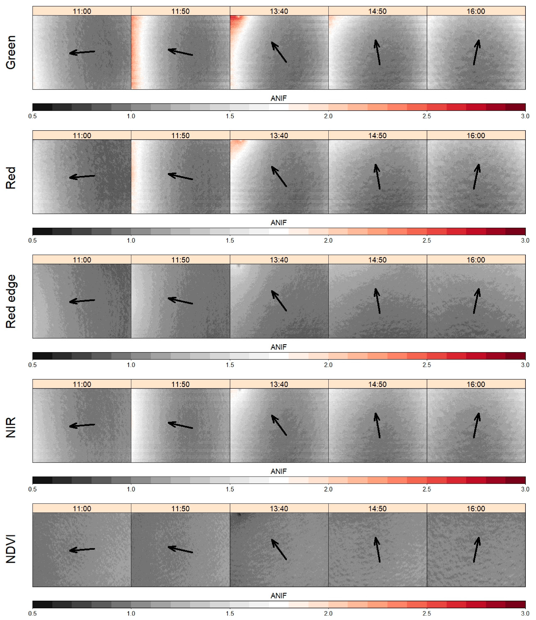
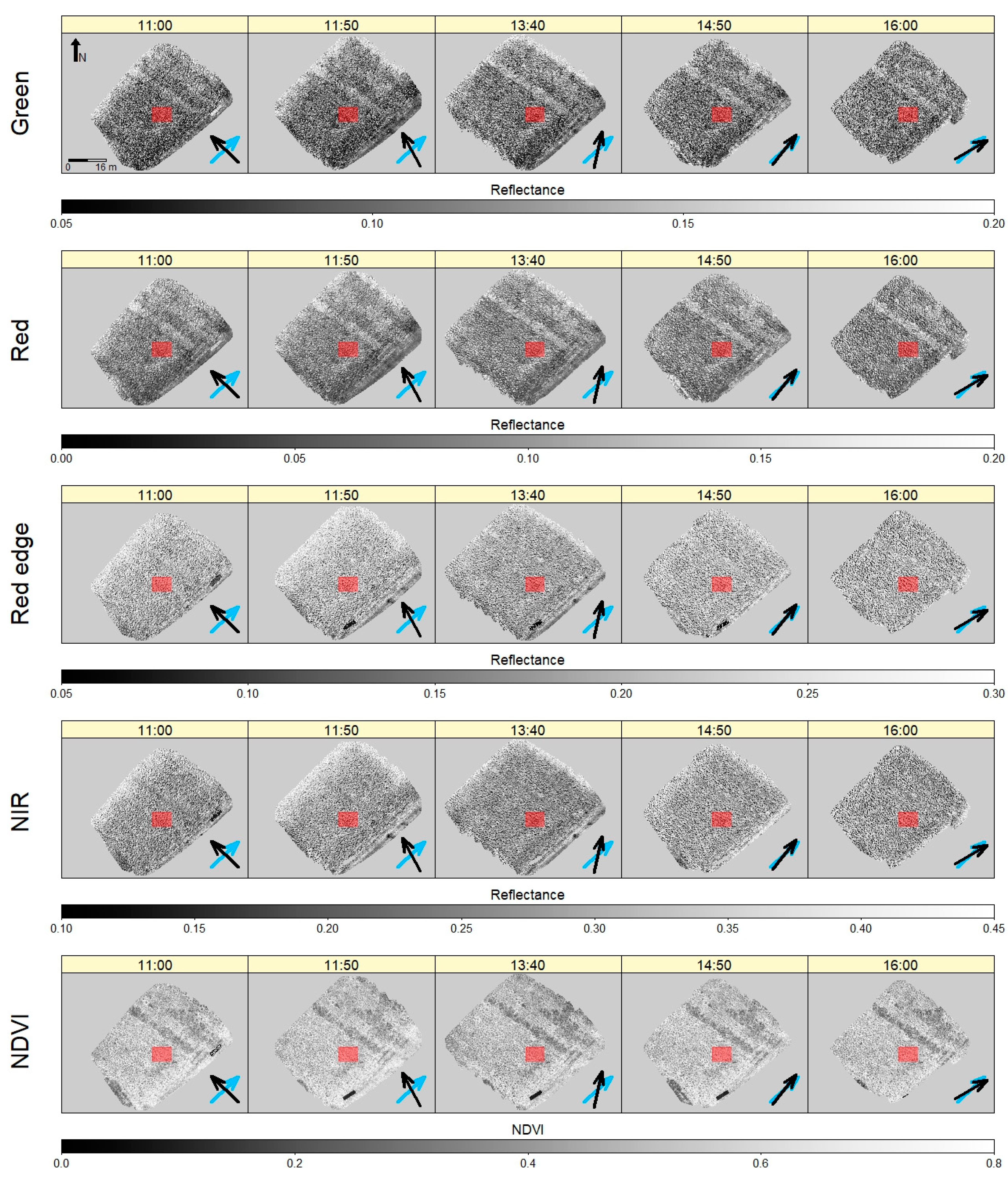
2.3.1. Illumination Geometry

To analyse the effect of illumination geometry on individual images, average reflectance images were calculated for each combination of band and flight time (i.e., using all images captured in one band over one flight). The number of images differed between flights, within a range of 389–489. This averaging was done to cancel out variation in the vegetation appearing in individual images, leaving an average variation in reflectance that was assumed to be due to anisotropic reflectance effects. Because skies were clear and flight times were short, illumination was as constant as possible over each set of images. The vegetation was reasonably homogeneous, though spatial variation in its reflectance properties could have had some effect on the average images.

A simplified anisotropy factor (sANIF) was then calculated for each pixel of these images. ANIF is the reflectance measured at a specific viewing and illumination geometry relative to the reflectance measured at nadir [23,25,26]. However, in this case the aim was to visualise the effect on averaged reflectance images. Viewing and illumination angles could not be calculated because these would have varied slightly at each pixel over each set of images used. It is therefore simplified here to the reflectance R of a pixel relative to the estimated reflectance R₀ at nadir (calculated as the mean reflectance in the region within a radius of 20 pixels from the image centre):

$$sANIF=\frac{R}{R_0}$$

The value of sANIF indicates how strongly reflectance or NDVI at a given pixel differs from the average at the image centre. The effect is to normalise the variations in reflectance across the averaged images so that visual comparisons can be made between bands.

To analyse the effect of illumination geometry on reflectance and NDVI maps from Pix4D, six regions of interest (ROIs) of the same shape and size (approximately 12 m²) were defined and the mean and standard deviation of reflectance/NDVI were calculated for each one, using QGIS 2.18.13 [43]. The ROIs were positioned away from the edges of the maps, covering vegetation with visually different NDVI properties. ROIs 1 and 2 contained vegetation with relatively low NDVIs; ROIs 3 and 4 had higher NDVIs and relatively low contrast between hummocks and hollows; ROIs 5 and 6 had higher contrast between hummocks and hollows (Figure 6).

Per-pixel differences were also calculated between each NDVI map and the NDVI map of the 13:40 flight. To reduce the effect of georeferencing errors (Section 2.2.2), each NDVI map was first resampled, using bilinear interpolation, to a GSD of 3.87 cm (three times the GSD of the 11:50 NDVI map, which had the coarsest resolution).

2.3.2. Flying Height

For each vertical profile flight, a 32 × 32 pixel region was defined that was filled by the tarp in all images. Mean reflectance in this region was calculated for each image and plotted against height above ground. This was calculated by subtracting the mean GPS altitude recorded by the Sequoia in images of the landing pad taken before and after the flight from the altitude recorded for each image during the flight.

2.3.3. Comparison between UAS and Ground Reference Data

Spectra from the ASD were averaged over a day (in the case of vegetation spectra), or over series of measurements taken at the same time (in the case of the tarp). These averaged spectra were then convolved to match the Sequoia bands. As the exact spectral response curve of the Sequoia was not available, it was assumed that its response is uniform within each band, so the ASD reflectance was simply averaged over the full width of each Sequoia band. The convolved ASD measurements were compared with:

• Mean reflectance in each Sequoia band from images collected above 25 m in vertical profile flights.
• Mean reflectance in each band in the six ROIs for reflectance maps of the 25-m flight and the 13:40 10-m flight on 14 May.

In each case, the set of ASD measurements taken closest to the flight time was used in the comparison, except for the second vertical profile flight on 7 June, where two sets of ASD measurements (approximately 30 min either side of the flight) were averaged.

3. Results

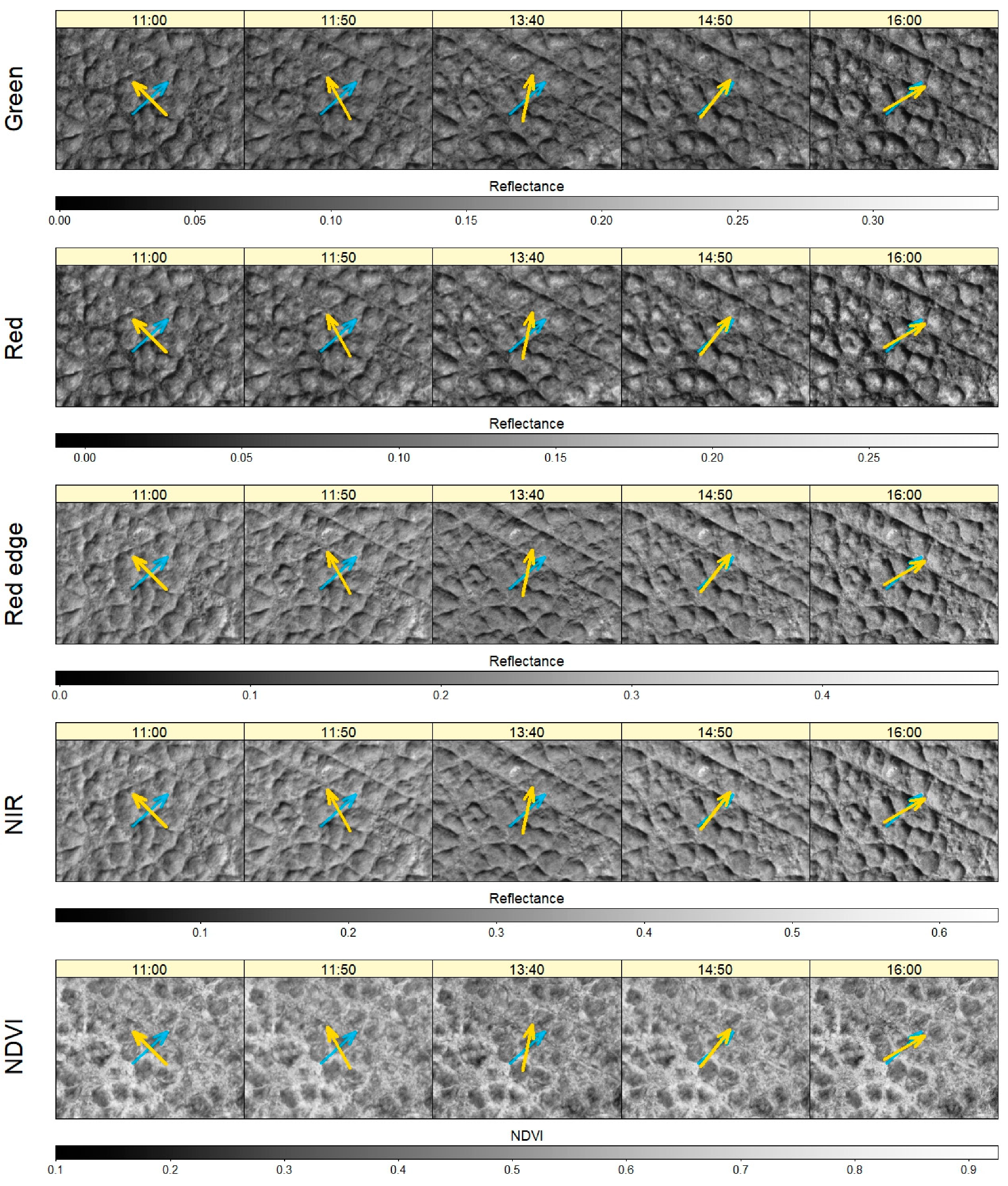
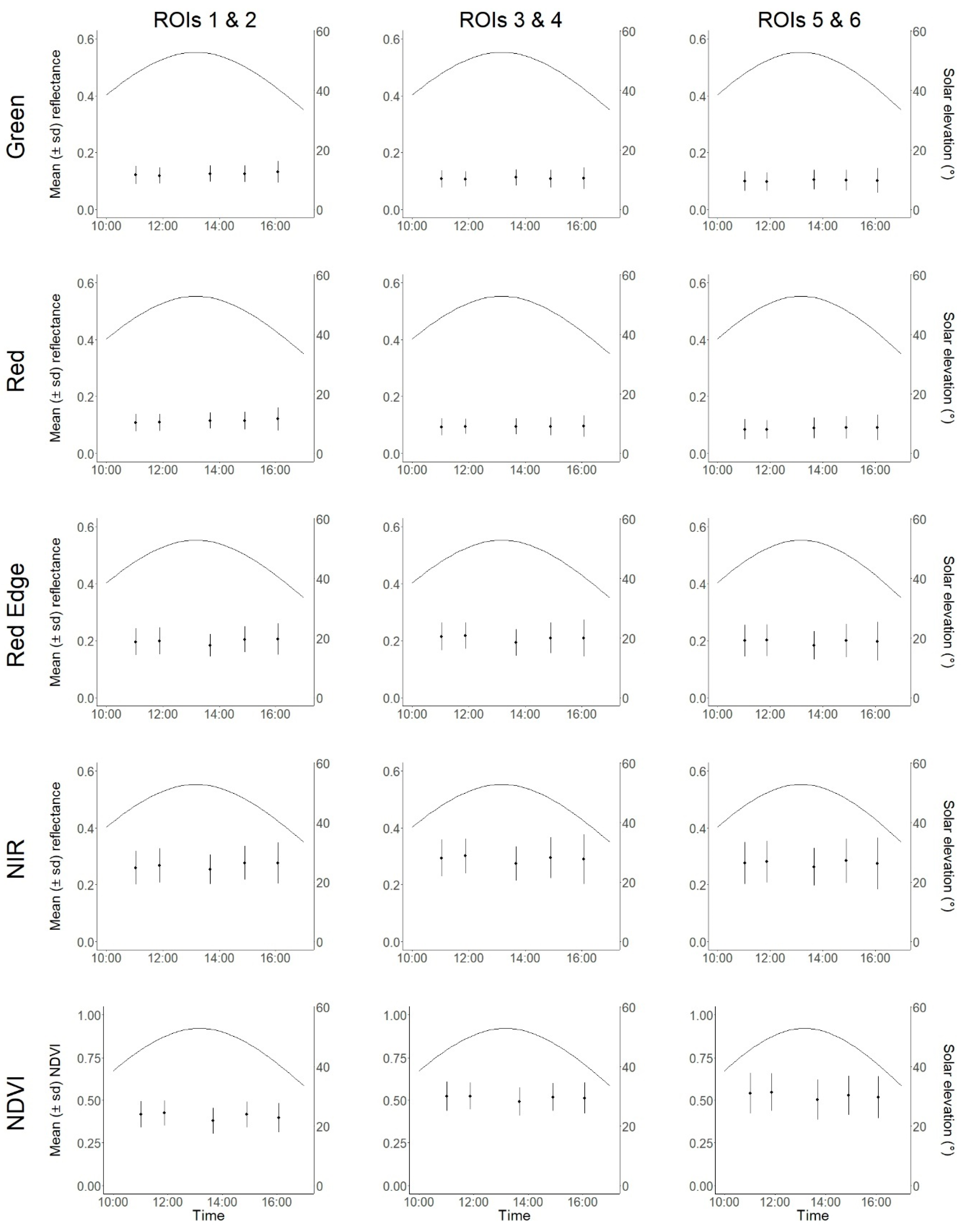
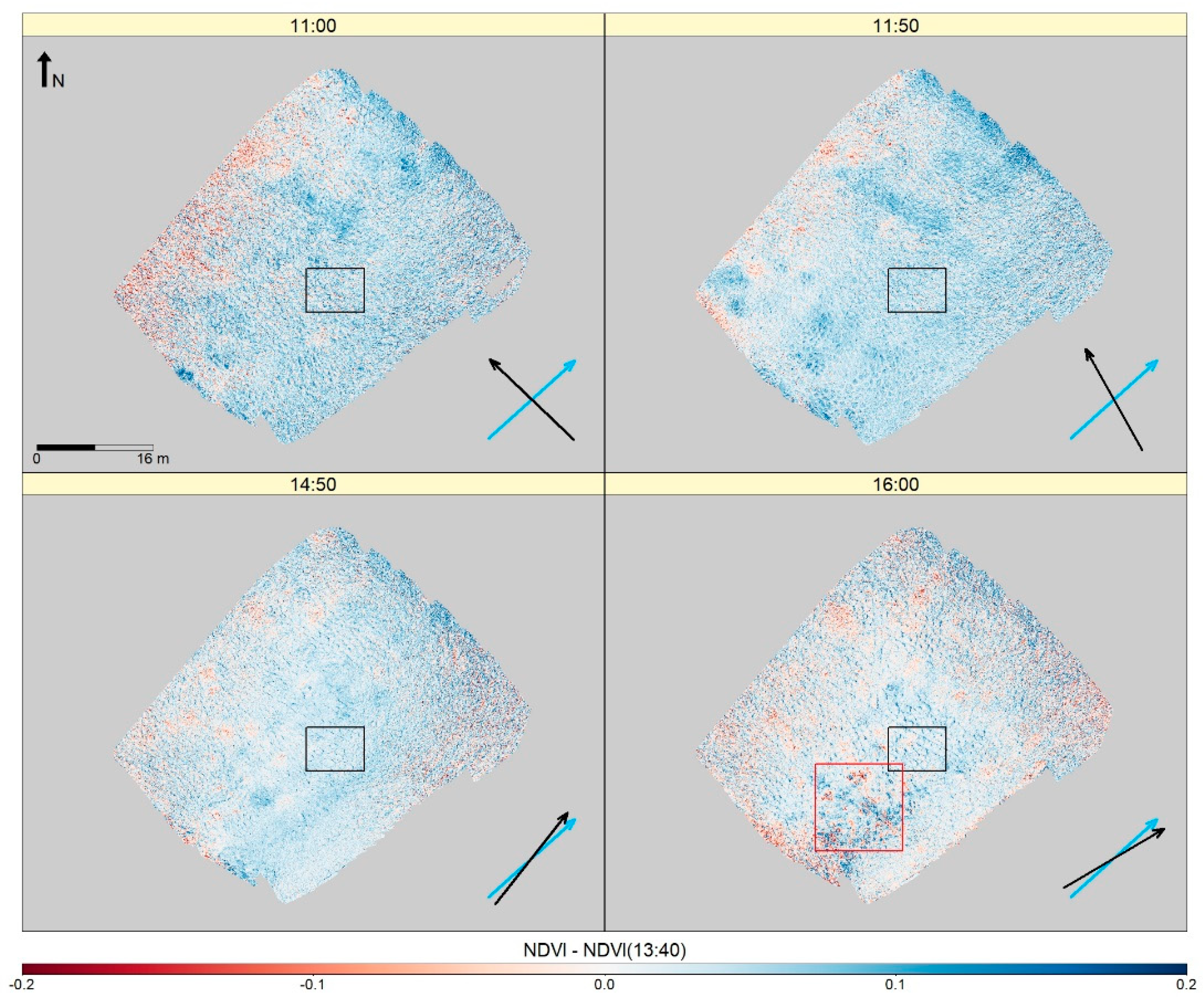
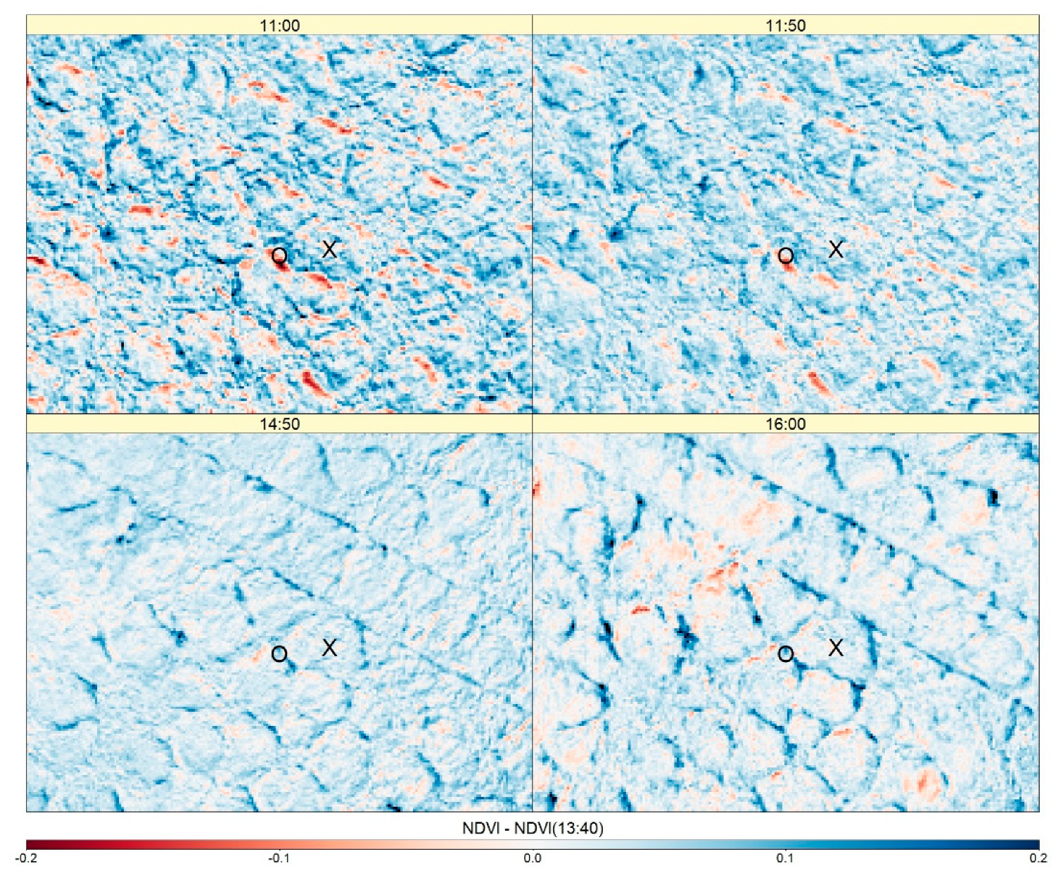
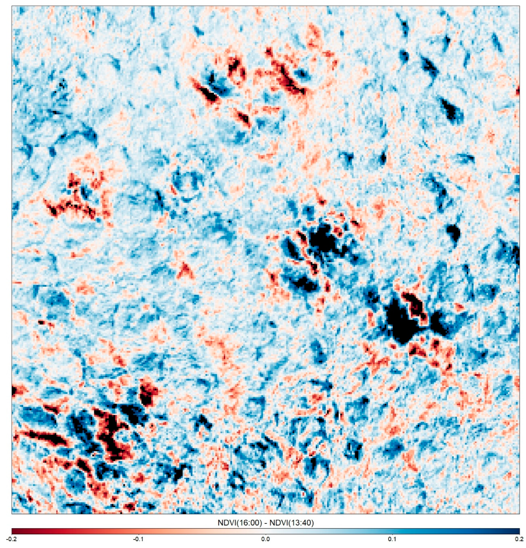
3.1. Effects of Illumination Geometry

Changing illumination geometry had a visible effect on reflectance in images from the 14 May flights (Figure 7). In the 13:40 flight, the hot spot was visible in the top left corner of the images, surrounding a small darker spot where the shadow of the UAS fell. In images from the other 10-m flights, the hot spot fell outside the Sequoia’s FOV, but there was still a noticeable increase in sANIF in the direction opposite the Sun, and an increase away from the image centre.

The relative strength of these two effects appeared to change over the day—in the morning the gradient in sANIF was predominantly right to left (i.e., increasing away from the Sun), while in the afternoon it was more circular (increasing away from the centre). The increase away from the centre was also slightly weaker in the Red band than in the NIR and Green bands.

Overall variation in sANIF was more pronounced in the Green and Red bands than in the NIR band, resulting in a slight decrease in NDVI away from the Sun (especially in the morning). Variation in sANIF across Red Edge images was less pronounced than in other bands, and variation in sANIF across NDVI images was smaller than across individual band images.

When images had been mosaiced in Pix4D, there was still an increase in reflectance in the direction opposite the Sun, but this effect was only visible at the edges of the reflectance maps (Figure 8). The 11:50 maps showed this edge effect most strongly, with higher reflectance along the NW and NE edges, and lower reflectance along the opposite edges. The 14:50 and 16:00 maps had much weaker edge effects, which is consistent with the change in the type of sANIF gradient between morning and afternoon images shown in Figure 7. Edge effects were much less visible in the NDVI maps, but there appeared to be a small decrease in NDVI at the NE edge of the 11:50 and 13:40 flights (Figure 8).

Reflectance in the NIR and Red Edge bands was noticeably lower in the 13:40 flight (which was closest to solar noon), while there was very little difference in the Green and Red bands. As a result, NDVI was lower in the 13:40 flight (Figure 9 and Figure 10). Contrast between well-illuminated and shadowed areas appeared to increase throughout the day, rather than showing an inverse relationship with solar elevation. The expected pattern appeared in the afternoon, with shadows increasing as solar elevation decreased. However, shadows appeared less strong in the morning than near noon.

The differences in mean NDVI were small—between 0.01 and 0.05. However, per-pixel differences were not spatially uniform and were much larger than mean differences in some areas (Figure 11, Figure 12 and Figure 13). This is partly because the flights did not cover the same area, which enhanced the edge effects described above. For example, the NW edge of the 11:00 and 11:50 NDVI maps overlapped with an area of the 13:40 map that was not near the edge, so NDVI was lower in this area of the 11:00 and 11:50 maps (Figure 11). There were other patches of above-average NDVI differences that appeared in both the 11:00 and 11:50 maps, suggesting that the effect of changing illumination on NDVI may vary with the vegetation—one of these patches was in the narrow strip of low NDVI running SE–NW across the survey area. Per-pixel NDVI differences also appeared to be smaller on the tops of hummocks than in hollows (Figure 12). The mean absolute per-pixel differences in NDVI from 13:40 were larger in the morning than the afternoon flights, with the 11:00 flight having the highest mean differences (

Table 4. The mean absolute per-pixel differences in NDVI between each flight and the 13:40 flight.

Flight Time	Mean Absolute NDVI Difference
11:00	0.0572
11:50	0.0484
14:50	0.0432
16:00	0.0445

).

In one area of the 16:00 map, the NDVI differences were as high as 0.5 for some pixels (Figure 13). However, this area looked somewhat blurred in the reflectance maps from the 16:00 flight, so this may have been related to motion blur or poor image overlap rather than to lower solar elevation.

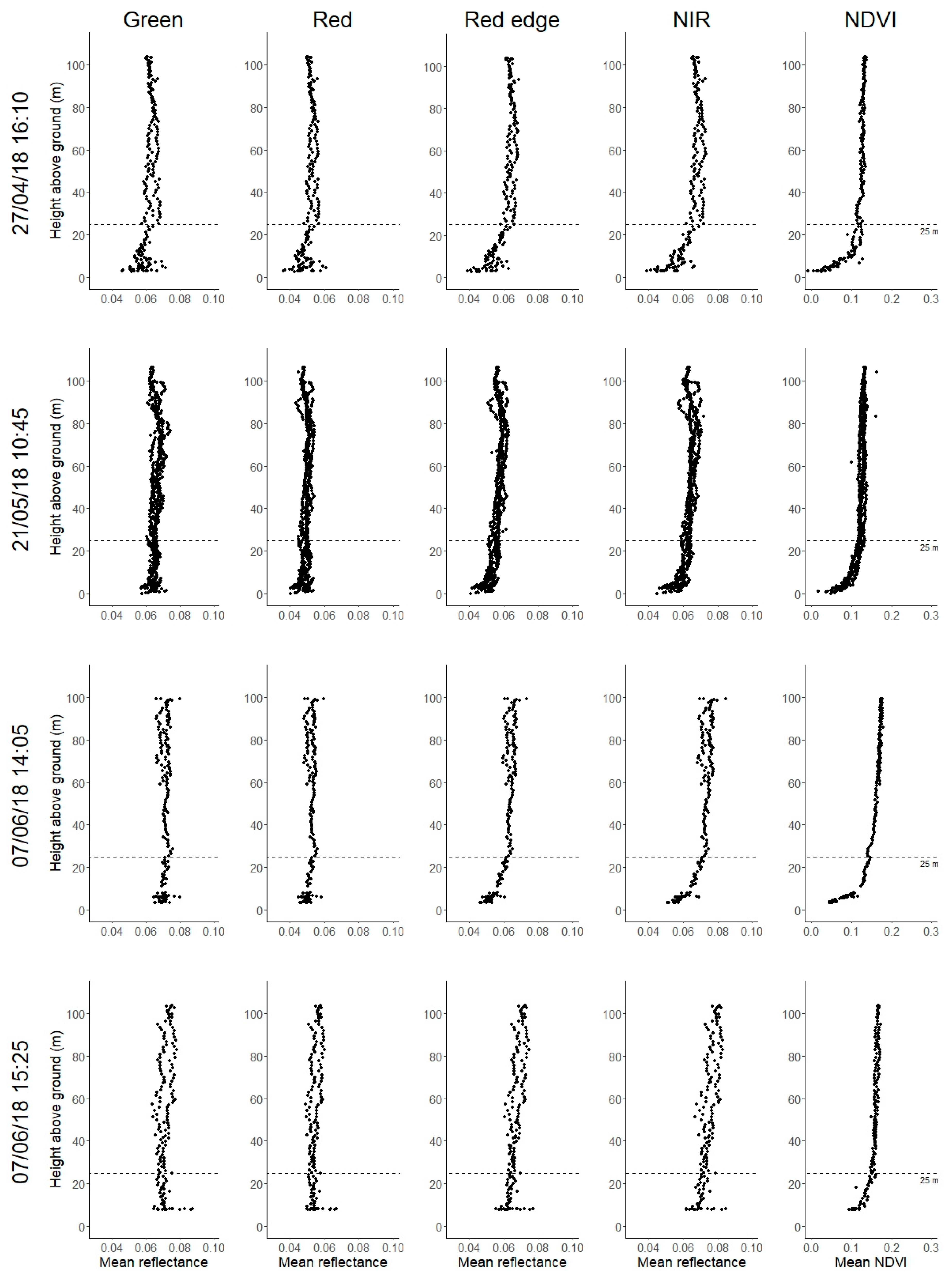
3.2. Effects of Flying Height

The effect of height above ground on the measured reflectance of the tarp varied between flights, but the general trend was an increase in Red Edge and NIR reflectance with height, especially in the first 25 m above ground. NDVI showed a similar trend, as the visible bands were much less affected by height than NIR (Figure 14). The greatest differences are seen in the NIR band (<0.04) and NDVI (<0.2) for 27 April, with most of the difference appearing in the first 25 m. There was also a small (<0.005) difference in reflectance between ascent and descent on 27 April and both 7 June flights, with higher reflectance values for the ascent in each case. Red and NIR bands were equally affected, so this effect was not apparent for NDVI.

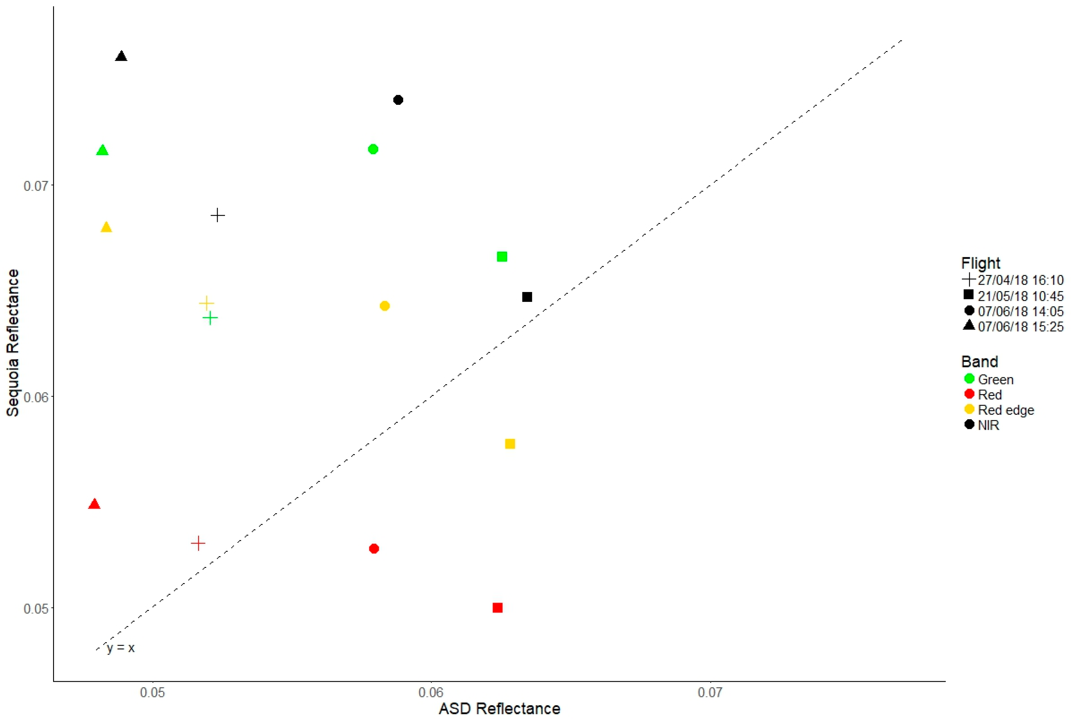
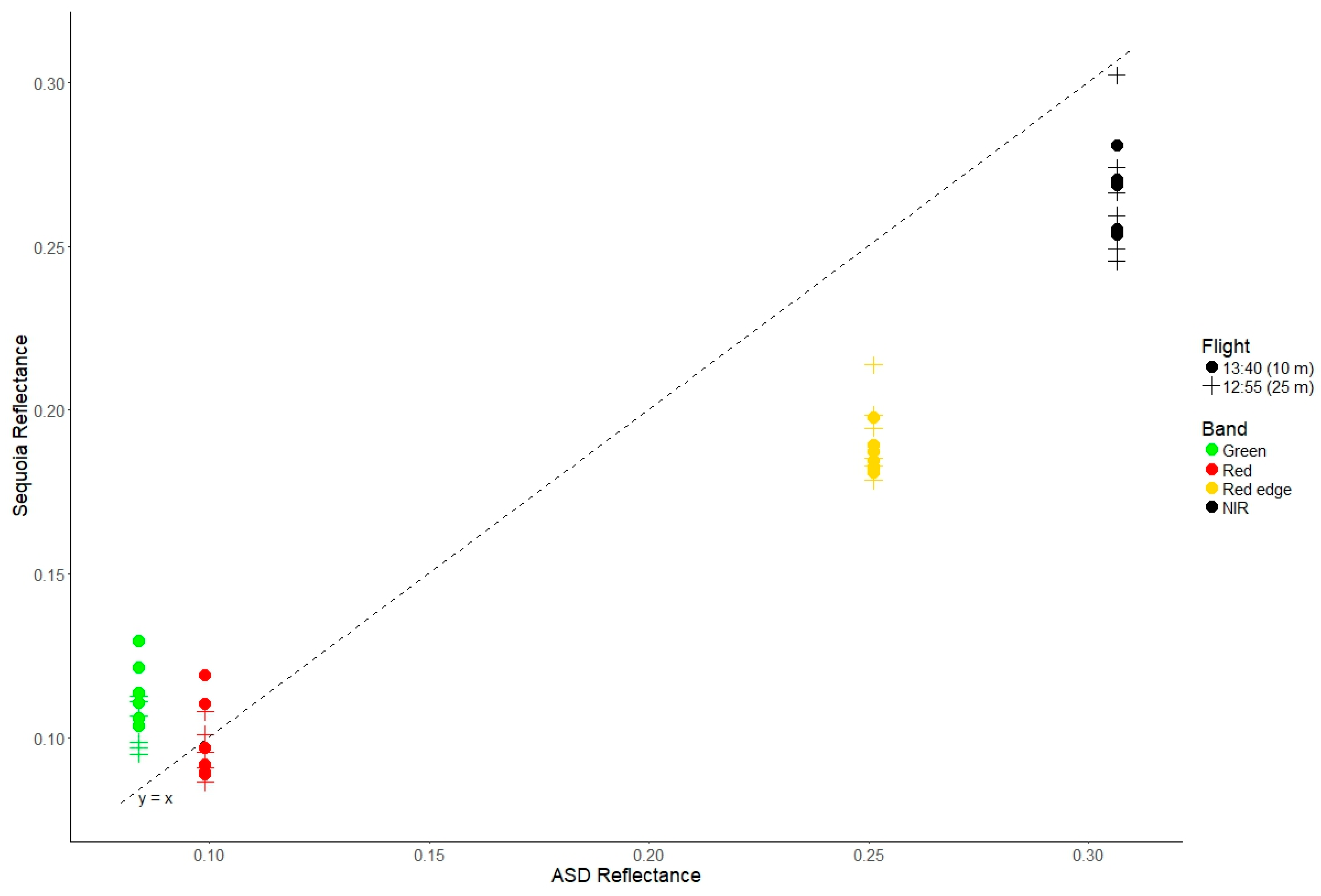
3.3. Comparison between Sequoia and Ground Reference Data

Comparison between the Sequoia and field spectrometer measurements revealed systematic discrepancies between the Sequoia’s bands (Figure 15 and Figure 16;

Table 5. Root mean square error (RMSE) values for comparisons among: ASD reflectance measurements; mean reflectance in ROIs in orthomosaics created from the 25-m and 13:40 10-m flights on 14 May; and Sequoia reflectance measurements of the large tarp.

Band	10 m vs. 25 m	Sequoia vs. ASD
		Vegetation			Tarp
		10-m Flights	25-m Flights	All Flights	All Flights
Green	0.0116	0.0315	0.0208	0.0267	0.0149
Red	0.0068	0.0114	0.0089	0.0103	0.0076
Red edge	0.0083	0.0642	0.0600	0.0621	0.0123
NIR	0.0098	0.0439	0.0444	0.0441	0.0176
NDVI	0.0193	0.0789	0.0621	0.0710	0.1394

). In Figure 15, the ASD reflectance associated with each vertical profile flight varies much less between bands than the Sequoia reflectance. The Sequoia appeared to overestimate in the Green, Red edge and NIR bands, except on 21 May. The Sequoia’s Red band measured consistently lower reflectance than the other bands, and stayed closer to the 1:1 line. (The lower Red reflectance is also apparent in Figure 14).

In the comparison between the ASD and vegetation reflectance maps (Figure 16), the Red band stayed close to the 1:1 line, while the Sequoia measured higher reflectance than the ASD in the Green band, but lower reflectance in Red edge and NIR bands. There was very little difference between the 10-m and 25-m flights.

Table 5 shows that the RMSE was much lower for comparisons of the Sequoia’s Red band and the ASD than for the equivalent comparisons among other bands. The RMSE for the comparisons of Sequoia and ASD was generally lower for the vertical profile flights over the tarp than for vegetation orthomosaics. The RMSE was also lower for the comparison between different heights than for the Sequoia versus ASD.

4. Discussion

This research investigated the effects of illumination geometry and flying height on imagery captured by a UAS with a multispectral sensor. The results showed that changing illumination geometry had visible effects on individual images, due to anisotropic reflectance of the vegetation. These effects were much less pronounced in orthomosaics, except where image overlap was lower at the edges of the survey area. Anisotropic reflectance effects should therefore be considered when planning UAS vegetation surveys. The effect of flying height was relatively minor, but comparison with ground reference data revealed discrepancies between the multispectral bands of the Sequoia, which may be problematic for comparisons with other sensors.

4.1. Anisotropic Reflectance

Several researchers have used UAS to measure the reflectance anisotropy of surfaces, using flight patterns designed to capture images or reflectance measurements of the same point from multiple angles [25,26,27,28]. A typical flight pattern of parallel lines with high overlap can also be used to measure reflectance anisotropy, by calculating the illumination and viewing angles of each pixel in images that have been aligned and orthorectified in photogrammetry software [19,24]. The method presented here is comparatively simple—whereas Roosjen et al. were able to visualise the spatial distribution of anisotropy parameters [24], our method only provides the average reflectance anisotropy of a small plot. Nevertheless, it is easy to apply, requires minimal processing time (<10 min per flight in this study) and allows the effect on individual images to be visualised (Figure 7), as opposed to variation with the viewing angle. However, it does rely on accurate vignette correction, as the greatest sANIF values are at the corners of the images, where vignetting is also greatest (Figure S1).

Two effects can be seen in Figure 7: an increase in sANIF in the backscattering direction, and an increase away from the image centre. The latter effect is caused by the sensor’s view penetrating further into the canopy at nadir than off-nadir, and a greater proportion of lower, more shaded layers can be seen in the nadir view, reducing apparent reflectance. The visible bands show a stronger backscattering effect than the NIR band because vegetation absorbs the visible wavelengths (especially red) more strongly than NIR, making the shadows darker relative to well-illuminated areas in the visible bands [23,44].

The relative influence of the two effects changed over the course of the day, with backscattering appearing stronger in the morning and the off-nadir effect stronger in the afternoon. This was less expected, as these effects are mainly related to solar zenith angle and canopy structure [23,44]. The contrast between well-illuminated and shadowed areas of orthomosaics also increased through the day (Figure 9). This may be at least partly explained by the drainage ditches running SE–NW across the site, which would have been more shadowed in the afternoon when the solar principal plane was perpendicular to them. The flight line orientation relative to the solar principal plane and the drainage ditches may also have had some effect, as the sensor’s FOV was not equal in all directions. Experiments with different flight lines at the same solar azimuth would be needed to investigate these potential interactions.

The apparent difference between hummocks and hollows in per-pixel NDVI comparisons (Figure 12) is interesting, as it suggests that the effect of illumination geometry on NDVI may vary over very short distances—for example, as a result of (micro)topography or vegetation type. The differences in NDVI appeared to be smaller on the hummocks, which would also have experienced smaller changes in illumination over the day than the hollows because they would be affected differently by shadows. The hummocks and hollows also had contrasting vegetation assemblages, whose reflectance properties could have responded differently to the change in illumination.

There is currently a need for reliable methods to correct for anisotropic reflectance effects in UAS images [19]. Figure 7 suggests that the use of vegetation indices may normalise these effects to some extent—the variation in sANIF across NDVI images is much smaller than across individual band images. Alternatively, average variations in sANIF could be used to normalise reflectance across images in individual bands. This is unlikely to be as accurate as methods that use 3D models of the surface [19], but would at least have the advantage of being quick and simple to apply. Unfortunately, this idea could not be tested as there was no way to validate the results against the ground reference data. Anisotropic reflectance effects were much less pronounced in the orthomosaics than in individual images, suggesting that Pix4D’s method for calculating pixel reflectance values is effective at correcting for these effects. One drawback is that the precise method of pixel averaging used by Pix4D is not known. This means that it is difficult (or impossible) to determine which pixels from which images were averaged, and it is not known what errors are introduced by the averaging [19].

It is worth emphasising that these results were specific to the phenological stage of the vegetation at the study site on the date they were surveyed, since anisotropic reflectance effects are strongly related to canopy structure. Another possible avenue of future research would be to repeat these measurements several times over a growing season, to determine how reflectance anisotropy changes over the phenological cycle at a certain site.

4.2. Flight Planning

Anisotropic reflectance effects became more pronounced towards the edges of orthomosaics, where image overlap was lower (Figure 8). This should be taken into consideration when planning UAS surveys. One solution is to fly in a grid pattern, rather than in parallel lines, to increase image overlap at the edges [13]. However, this may not be practical for large surveys where time or batteries are limited. An alternative is simply to allow a reasonable buffer around the area of interest, so that it is less likely to be near the edge. The buffer may need to be large if per-pixel comparisons are to be attempted, because no two flights will cover exactly the same area, and the edge of one may overlap the middle of another.

NDVI was lower in the flight nearest solar noon, which agrees with the trend observed by Brede et al. in UAS surveys of a tropical rainforest ecosystem [30]. Ishihara et al. found a similar effect, sometimes with a sharp drop at solar noon, in continuous ground-based measurements of three types of cropland in Japan [45]. On the other hand, Assmann et al. found an increase in NDVI with solar elevation [13], suggesting that the NDVI response may be site-specific. One possibility is that the presence of the hot spot within the FOV of the sensor causes NDVI to decrease. This happened by chance in the 13:40 flight on 14 May—the approximate solar zenith angle was 37.6° and the diagonal FOV of the sensor was 36.9° either side of nadir (Table 1). The flight line orientation made it just possible for the hot spot to appear in the corner (Figure 7). The results reported by Assmann et al. were for a site in the Canadian Arctic, and solar elevation was lower [13], so the hot spot would not have been within the FOV of the sensor. This hypothesis would need more investigation, but if confirmed it would suggest that flights should be planned to avoid hot spots appearing in images. However, this may be difficult at low latitudes.

4.3. Flying Height

The results relating to flying height were inconclusive. The increase in NDVI of the large tarp with height was more pronounced in some flights than in others (Figure 14), and there was no consistent effect of flying height on vegetation reflectance in orthomosaics (Figure 16). There was an interesting difference between individual images captured on the ascent and on the descent in vertical profile flights, with the ascent having higher reflectance values over a range of heights. This is difficult to explain, but probably not relevant for most applications, as images are generally captured from a constant flying height. One factor that might have influenced these measurements was downdraft from the UAS causing ripples to form in the fabric, possibly changing its apparent reflectance. This might explain the increased variability in reflectance in the first few metres above ground (Figure 14), but probably not the whole trend up to 25 m.

4.4. Radiometric Calibration

Although it is not possible to say from these results whether there was any atmospheric effect, they do raise questions about radiometric calibration. If calibration images are taken on the ground, then any change in measured reflectance with height is ignored; if images of the tarp had been used for calibration, this would have slightly changed the relationship between Red and NIR bands, and thus NDVI. There are also discrepancies between bands apparent in the comparisons with ground reference data (Figure 15 and Figure 16). It is not known what caused these discrepancies, or whether they are unique to the Sequoia unit used. This is a potential source of uncertainty in comparisons with other sensors, including other Sequoia units, and illustrates the value of using in-flight reflectance targets for quality control [13,19].

5. Conclusions

This research has demonstrated that illumination geometry and flying height can affect the retrieval of reflectance values from individual images acquired by UAS, but that photogrammetry and the use of vegetation indices such as NDVI can mitigate the effects of illumination geometry. These effects are specific to individual flights, since they depend on changing solar geometry, canopy structure and possibly atmospheric composition. Measurements of anisotropic reflectance and flying height effects at a greater variety of sites will hopefully lead to a better understanding of these issues and more robust radiometric calibration procedures, increasing the quality of UAS data products and making them more comparable across sites, sensors and times.

References

1. Manfreda, S.; McCabe, M.F.; Miller, P.E.; Lucas, R.; Pajuelo Madrigal, V.; Mallinis, G.; Ben Dor, E.; Helman, D.; Estes, L.; Ciraolo, G.; et al. On the Use of Unmanned Aerial Systems for Environmental Monitoring. Remote Sens. 2018, 10, 641. [Google Scholar] [CrossRef]
2. Cruzan, M.B.; Weinstein, B.G.; Grasty, M.R.; Kohrn, B.F.; Hendrickson, E.C.; Arredondo, T.M.; Thompson, P.G. Small unmanned aerial vehicles (micro-UAVs, drones) in plant ecology. Appl. Plant Sci. 2016, 4, 1600041. [Google Scholar] [CrossRef] [PubMed]
3. Anderson, K.; Gaston, K.J. Lightweight unmanned aerial vehicles will revolutionize spatial ecology. Front. Ecol. Environ. 2013, 11, 138–146. [Google Scholar] [CrossRef] [Green Version]
4. Pádua, L.; Vanko, J.; Hruška, J.; Adão, T.; Sousa, J.J.; Peres, E.; Morais, R. UAS, sensors, and data processing in agroforestry: A review towards practical applications. Int. J. Remote Sens. 2017, 38, 2349–2391. [Google Scholar] [CrossRef]
5. Torresan, C.; Berton, A.; Carotenuto, F.; Gennaro, S.F.D.; Gioli, B.; Matese, A.; Miglietta, F.; Vagnoli, C.; Zaldei, A.; Wallace, L. Forestry applications of UAVs in Europe: A review. Int. J. Remote Sens. 2017, 38, 2427–2447. [Google Scholar] [CrossRef]
6. Salamí, E.; Barrado, C.; Pastor, E. UAV flight experiments applied to the remote sensing of vegetated areas. Remote Sens. 2014, 6, 11051–11081. [Google Scholar] [CrossRef]
7. Zhang, C.; Kovacs, J.M. The application of small unmanned aerial systems for precision agriculture: A review. Precis. Agric. 2012, 13, 693–712. [Google Scholar] [CrossRef]
8. Cowley, D.; Moriarty, C.; Geddes, G.; Brown, G.; Wade, T.; Nichol, C. UAVs in Context: Archaeological Airborne Recording in a National Body of Survey and Record. Drones 2017, 2, 2. [Google Scholar] [CrossRef]
9. Singh, K.K.; Frazier, A.E. A meta-analysis and review of unmanned aircraft system (UAS) imagery for terrestrial applications. Int. J. Remote Sens. 2018. [Google Scholar] [CrossRef]
10. Aasen, H.; Honkavaara, E.; Lucieer, A.; Zarco-Tejada, P.J. Quantitative Remote Sensing at Ultra-High Resolution with UAV Spectroscopy: A Review of Sensor Technology, Measurement Procedures, and Data Correction Workflows. Remote Sens. 2018, 10, 1091. [Google Scholar] [CrossRef]
11. Dandois, J.; Olano, M.; Ellis, E. Optimal Altitude, Overlap, and Weather Conditions for Computer Vision UAV Estimates of Forest Structure. Remote Sens. 2015, 7, 13895–13920. [Google Scholar] [CrossRef] [Green Version]
12. Kelcey, J.; Lucieer, A. Sensor Correction of a 6-Band Multispectral Imaging Sensor for UAV Remote Sensing. Remote Sens. 2012, 4, 1462–1493. [Google Scholar] [CrossRef] [Green Version]
13. Assmann, J.J.; Kerby, J.T.; Cunliffe, A.M.; Myers-Smith, I.H. Vegetation monitoring using multispectral sensors - best practices and lessons learned from high latitudes. bioRxiv 2018. [Google Scholar] [CrossRef]
14. Berra, E.F.; Gaulton, R.; Barr, S. Commercial Off-the-Shelf Digital Cameras on Unmanned Aerial Vehicles for Multitemporal Monitoring of Vegetation Reflectance and NDVI. IEEE Trans. Geosci. Remote Sens. 2017, 55, 4878–4886. [Google Scholar] [CrossRef] [Green Version]
15. Lebourgeois, V.; Bégué, A.; Labbé, S.; Mallavan, B.; Prévot, L.; Roux, B. Can Commercial Digital Cameras Be Used as Multispectral Sensors? A Crop Monitoring Test. Sensors 2008, 8, 7300–7322. [Google Scholar] [CrossRef]
16. Lelong, C.C.D.; Burger, P.; Jubelin, G.; Roux, B.; Labbé, S.; Baret, F. Assessment of Unmanned Aerial Vehicles Imagery for Quantitative Monitoring of Wheat Crop in Small Plots. Sensors 2008, 8, 3557–3585. [Google Scholar] [CrossRef]
17. Smith, G.M.; Milton, E.J. The use of the empirical line method to calibrate remotely sensed data to reflectance. Int. J. Remote Sens. 1999, 20, 2653–2662. [Google Scholar] [CrossRef]
18. Wang, C.; Myint, S.W. A Simplified Empirical Line Method of Radiometric Calibration for Small Unmanned Aircraft Systems-Based Remote Sensing. IEEE J. Sel. Top. Appl. Earth Obs. Remote Sens. 2015, 8, 1876–1885. [Google Scholar] [CrossRef]
19. Aasen, H.; Bolten, A. Multi-temporal high-resolution imaging spectroscopy with hyperspectral 2D imagers—From theory to application. Remote Sens. Environ. 2018, 205, 374–389. [Google Scholar] [CrossRef]
20. Domenzain, L. Reflectance Estimation. Available online: https://forum.developer.parrot.com/t/reflectance-estimation/5597/2 (accessed on 3 May 2018).
21. Parrot Drones SAS. Application note: Pixel value to irradiance using the sensor calibration model. Available online: https://forum.developer.parrot.com/uploads/default/original/2X/3/383261d35e33f1f375ee49e9c7a9b10071d2bf9d.pdf (accessed on 3 May 2018).
22. Ortega-Terol, D.; Hernandez-Lopez, D.; Ballesteros, R.; Gonzalez-Aguilera, D. Automatic Hotspot and Sun Glint Detection in UAV Multispectral Images. Sensors 2017, 17, 2352. [Google Scholar] [CrossRef]
23. Sandmeier, S.; Müller, C.; Hosgood, B.; Andreoli, G. Physical Mechanisms in Hyperspectral BRDF Data of Grass and Watercress. Remote Sens. Environ. 1998, 66, 222–233. [Google Scholar] [CrossRef]
24. Roosjen, P.P.J.; Suomalainen, J.M.; Bartholomeus, H.M.; Kooistra, L.; Clevers, J.G.P.W. Mapping Reflectance Anisotropy of a Potato Canopy Using Aerial Images Acquired with an Unmanned Aerial Vehicle. Remote Sens. 2017, 9, 417. [Google Scholar] [CrossRef]
25. Roosjen, P.P.J.; Suomalainen, J.M.; Bartholomeus, H.M.; Clevers, J.G.P.W. Hyperspectral Reflectance Anisotropy Measurements Using a Pushbroom Spectrometer on an Unmanned Aerial Vehicle—Results for Barley, Winter Wheat, and Potato. Remote Sens. 2016, 8, 909. [Google Scholar] [CrossRef]
26. Burkart, A.; Aasen, H.; Alonso, L.; Menz, G.; Bareth, G.; Rascher, U. Angular Dependency of Hyperspectral Measurements over Wheat Characterized by a Novel UAV Based Goniometer. Remote Sens. 2015, 7, 725–746. [Google Scholar] [CrossRef] [Green Version]
27. Grenzdörffer, G.J.; Niemeyer, F. UAV Based BRDF-Measurements of Agricultural Surfaces with PFIFFikus. ISPRS - Int. Arch. Photogramm. Remote Sens. Spat. Inf. Sci. 2012, XXXVIII-1/C22, 229–234. [Google Scholar]
28. Hakala, T.; Suomalainen, J.; Peltoniemi, J.I. Acquisition of Bidirectional Reflectance Factor Dataset Using a Micro Unmanned Aerial Vehicle and a Consumer Camera. Remote Sens. 2010, 2, 819–832. [Google Scholar] [CrossRef] [Green Version]
29. Rasmussen, J.; Ntakos, G.; Nielsen, J.; Svensgaard, J.; Poulsen, R.N.; Christensen, S. Are vegetation indices derived from consumer-grade cameras mounted on UAVs sufficiently reliable for assessing experimental plots? Eur. J. Agron. 2016, 74, 75–92. [Google Scholar] [CrossRef]
30. Brede, B.; Suomalainen, J.; Bartholomeus, H.; Herold, M. Influence of solar zenith angle on the enhanced vegetation index of a Guyanese rainforest. Remote Sens. Lett. 2015, 6, 972–981. [Google Scholar] [CrossRef]
31. Yu, X.; Liu, Q.; Liu, X.; Liu, X.; Wang, Y. A physical-based atmospheric correction algorithm of unmanned aerial vehicles images and its utility analysis. Int. J. Remote Sens. 2017, 38, 3101–3112. [Google Scholar] [CrossRef]
32. NERC Centre for Ecology & Hydrology. Auchencorth Moss Fieldsite. Available online: http://www.auchencorth.ceh.ac.uk/ (accessed on 7 March 2018).
33. NERC Centre for Ecology & Hydrology. Auchencorth Moss: An atmospheric observatory. Available online: https://www.ceh.ac.uk/our-science/monitoring-site/auchencorth-moss-atmospheric-observatory (accessed on 7 March 2018).
34. Parrot Drones SAS. Parrot Sequoia. Available online: https://www.parrot.com/uk/parrot-professional/parrot-sequoia (accessed on 7 March 2018).
35. NERC Field Spectroscopy Facility. Field Guide for the ASD FieldSpec Pro – White Reference Mode. Available online: http://fsf.nerc.ac.uk/resources/guides/pdf_guides/asd_guide_v2_wr.pdf (accessed on 23 April 2018).
36. R Core Team. R: A Language and Environment for Statistical Computing; R Foundation for Statistical Computing: Vienna, Austria, 2018. [Google Scholar]
37. Hijmans, R. raster: Geographic Data Analysis and Modeling. 2017. Available online: https://cran.r-project.org/package=raster (accessed on 3 May 2018).
38. Parrot Drones SAS. Application note: How to correct vignetting in images. Available online: https://forum.developer.parrot.com/uploads/default/original/2X/b/b9b5e49bc21baf8778659d8ed75feb4b2db5c45a.pdf (accessed on 3 May 2018).
39. Domenzain, L. Details of Irradiance List tag for Sunshine sensor in exif data of Sequoia. Available online: https://forum.developer.parrot.com/t/details-of-irradiance-list-tag-for-sunshine-sensor-in-exif-data-of-sequoia/5261/2 (accessed on 3 May 2018).
40. Bashir, M. How to convert Sequoia images to reflectance? Available online: https://onedrive.live.com/?authkey=%21ACzNLk1ORe37aRQ&cid=C34147D823D8DFEF&id=C34147D823D8DFEF%2115414&parId=C34147D823D8DFEF%21106&o=OneUp (accessed on 3 May 2018).
41. Pix4D SA. Radiometric corrections. Available online: https://support.Pix4D.com/hc/en-us/articles/202559509 (accessed on 7 March 2018).
42. Agafonkin, V.; Thieurmel, B. suncalc: Compute Sun Position, Sunlight Phases, Moon Position and Lunar Phase, R package version 0.4; 2018. Available online: https://CRAN.R-project.org/package=suncalc (accessed on 3 May 2018).
43. QGIS Development Team. QGIS Geographic Information System. Open Source Geospatial Foundation Project. 2017. Available online: http://www.qgis.org (accessed on 3 May 2018).
44. Kimes, D.S. Dynamics of directional reflectance factor distributions for vegetation canopies. Appl. Opt. 1983, 22, 1364–1372. [Google Scholar] [CrossRef]
45. Ishihara, M.; Inoue, Y.; Ono, K.; Shimizu, M.; Matsuura, S. The Impact of Sunlight Conditions on the Consistency of Vegetation Indices in Croplands—Effective Usage of Vegetation Indices from Continuous Ground-Based Spectral Measurements. Remote Sens. 2015, 7, 14079–14098. [Google Scholar] [CrossRef]
Figure 1. Workflow diagrams for analysis of (a) illumination geometry effects and (b) flying height effects and comparison with ground reference data. sANIF refers to the simplified anisotropy factor (described in Section 2.3.1).
Drones 03 00055 g001
Figure 2. Map showing location of Auchencorth Moss, with study area outlined in yellow. Main map: image Copyright 2018 DigitalGlobe, Getmapping plc; map data Copyright 2018 Google. Inset map: Map tiles by Stamen Design, under CC BY 3.0. Data by OpenStreetMap, under ODbL.
Drones 03 00055 g002
Figure 3. RGB orthomosaic of (a) the study site and (b) the area surveyed from a height of 10 m on 14 May 2018 (outlined in black).
Drones 03 00055 g003
Figure 4. Photograph of the UAS and landing pad during take-off. Copyright D. Stow.
Drones 03 00055 g004
Figure 5. Photograph of the rig used for capturing calibration images. Copyright D. Stow.
Drones 03 00055 g005
Figure 6. NDVI map from the 10-m flight at 13:40 on 14 May, showing the ROIs used to analyse differences in reflectance and NDVI between flights. The rectangular extent of this figure is the same as the extent outlined in black in Figure 3. The low NDVI rectangle to the south of the image is a small black tarp that was placed as an in-flight calibration target but is not relevant to the results presented here.
Drones 03 00055 g006
Figure 7. Variation in simplified anisotropy factor (sANIF) in images averaged across each Sequoia band in each 10-m flight on 14 May, and in NDVI images calculated from the averaged Red and NIR images. The solar principal plane is indicated by the arrows, which point away from the Sun. The value of sANIF indicates how strongly reflectance or NDVI at a given pixel differs from the average at the image centre (a sANIF of 1 indicates equality).
Drones 03 00055 g007
Figure 8. Reflectance and NDVI maps produced by Pix4Dmapper for each 10-m flight on 14 May. The solar principal plane is indicated by the black arrows, which point away from the Sun. The blue arrows show the approximate orientation of Sequoia images (rotated 48° clockwise from north). The red shaded area is shown in more detail in Figure 9.
Drones 03 00055 g008
Figure 9. Images of a small (8 × 6 m) extract from the reflectance and NDVI maps (shaded in red in Figure 8). The solar principal plane is indicated by the yellow arrows, which point away from the Sun. The blue arrows show the approximate orientation of Sequoia images.
Drones 03 00055 g009
Figure 10. Plots of mean (±s.d.) reflectance in each band (and NDVI) in pairs of ROIs over the 10-m flights on 14 May. The curve shows the change in solar elevation over the day. Each pair of ROIs had similar NDVI properties (Figure 6) and showed a similar response to solar elevation.
Drones 03 00055 g010
Figure 11. Per-pixel differences in NDVI between the 13:40 flight and the other 10-m flights on 14 May. The areas outlined in black and red are shown in Figure 12 and Figure 13, respectively. The arrows indicate the solar principal plane (black) and orientation of the camera (blue), as in Figure 8.
Drones 03 00055 g011
Figure 12. Per-pixel NDVI differences in the 8 × 6 m area shown in Figure 9 (outlined in black in Figure 11). X = example hummock; O = example hollow.
Drones 03 00055 g012
Figure 13. Per-pixel NDVI differences between the 16:00 and 13:40 flights in the area outlined in red in Figure 11. Differences outside the range ±0.2 NDVI are shown in black.
Drones 03 00055 g013
Figure 14. Variation in the measured reflectance and NDVI of the tarp with the height of the Sequoia above ground, plotted as separate vertical profiles for each band during each flight.
Drones 03 00055 g014
Figure 15. Comparison between measurements of the reflectance of the large tarp from the ASD FieldSpec Pro and the Sequoia. Reflectance spectra measured by the ASD at the times closest to each flight were averaged and convolved to match the Sequoia bands. Reflectance measured by the Sequoia was averaged over all images captured from above 25 m in a single vertical profile flight. A 1:1 line is plotted for comparison.
Drones 03 00055 g015
Figure 16. Comparison between vegetation reflectance measurements taken on 14 May 2018 by the ASD FieldSpec Pro and the Sequoia. Reflectance spectra measured by the ASD were averaged and convolved to match the Sequoia bands. Each point shows the mean Sequoia reflectance in one of the six ROIs in Pix4D reflectance maps from the 25-m flight and the 13:40 10-m flight. A 1:1 line is plotted for comparison.
Drones 03 00055 g016