1. Introduction
Small multirotor Unmanned Aerial Systems (sUAS), often referred to as drones, have vertical takeoff and landing (VTOL) capabilities along with good maneuverability that make them an important asset for many applications. They have received unprecedented attention in the past decade due to their adoption in military usage [
1], civil applications [
2], and scientific research applications [
3,
4]. Most studies on multirotor sUAS focus on control and photography functions [
5] while little research is related to aerodynamics or aeroacoustics. Although the case, aerodynamics, and aeroacoustics of multirotor sUAS should not be disregarded. Multirotor UAS using rechargeable batteries are predicted to have a maximum endurance between 30 and 40 minutes depending on their disc loading and forward flight speed, placing a precedence on aerodynamic efficiency [
6,
7]. Data collected by Leishman [
8] showed that the small-scale rotors used on these systems have a lowered figure of merit, or the ratio of ideal power required to actual power required, compared to rotors on full-scale helicopters. This finding is due to the lower Reynolds number regime that small-scale rotors operate at, meaning viscous forces are more dominant. In this case, figure of merit is an aerodynamic performance metric that is proportional to endurance. In terms of acoustics, the applications previously mentioned typically put sUAS in close proximity to humans, potentially causing annoyance due to emitted noise. It is shown in [
9] that a quadrotor UAS weighing 2.1 Kg can produce an overall sound pressure level A-weighting (OASPLA) between 45 and 65 dBA when 35 to 5 meters away, respectively. According to a psychoacoustic study [
10], these overall SPLs would cause the majority of people to be slightly to moderately annoyed. Similarly, it has been shown that drone noise can cause detrimental effects on various animals, a common occurrence due to agriculture and wildlife imagery tasks carried out by drones [
3,
11]. Due to the previously discussed topics, aerodynamic and acoustic performances become prominent issues likely to affect the design and usage of UAS. Furthermore, it is critical to accurately predict and understand the flow and acoustic characteristics of these systems in order for a more aerodynamically efficient and quiet design to be created.
While aerodynamic performance metrics such as thrust coefficient and power coefficient are important quantitative metrics, they do not provide information on why some rotor geometries are more aerodynamically efficient. In order to better understand why certain performance values are obtained, a form of flow visualization must be used to view the flow characteristics in the wake. Likewise, observing or calculating surface pressures can be used to provide qualitative insights. Past research using smoke flow visualization shows why low Reynolds number rotors are less efficient [
12,
13]. From the visualization, it is shown that thick wake sheets are produced from the rotors which wander to the center of the wake, causing possible obstruction of the axial velocity. The root portion of the wake sheet was also convected less into the wake, proving that insufficient inflow is produced by this region of the rotor. The shed tip vortices are large and strong relative to the rotor’s size and thrust, suggesting that there is considerable downwash and induced drag occurring at this location. Lastly, the wake produced by the rotor contracts significantly; by using one dimensional momentum theory, it can be shown that this attribute causes a reduction in aerodynamic efficiency [
8]. While there has been much research investigating isolated small-scale rotors, not much attention has been put on rotor–airframe interactions. Yoon et al. [
14] found that there is little difference in thrust production when rotors are mounted above or below the airframe. It was also found that when the rotors were mounted below, there were significant unsteady variations in pressure on the airframe.
Like aerodynamic performance, the acoustic performance of rotors is also affected by the Reynolds number. Isolated low Reynolds number rotors are dominated by tonal noise in the low to mid frequency range, similar to full-scale rotors [
2]. At higher frequencies, it is shown that broadband noise is significant for low Reynolds number rotors [
15,
16]. A computational study revealed that broadband noise is significant at higher frequencies at locations in and out of the rotor plane [
17]. This study also showed that noise due to fluid displacement, also known as thickness noise, contributes no noise to a receiver directly above the rotor plane. It was found that above plane noise is dominated by loading and broadband sources. Conversely, in plane noise was found to be affected by all noise sources—thickness, loading, and quadrupole. This same study showed that noise caused by an airframe placed underneath the rotor is significant and that there is up to an 8 dBA (A-weighted sound pressure level) difference in overall sound pressure level when the location of the receiver in the plane of the rotor was altered. If an airframe was not included in the model, the noise at all in plane locations would be the same. It is also acknowledged that airframe noise seems to affect the mid frequencies, between 400 and 1500 Hz, the most [
17]. Furthermore, noise from a cylinder in steady crossflow, which is analogous to a cylindrical airframe in the wake of a rotor, produces peaks in noise typically between 400 and 700 Hz, or at the frequency that the lift coefficient is varying [
18]. It was found that receiver locations that experienced the greatest noise were normal to portions of the cylinder that experienced the greatest pressure fluctuations. From a study conducted at NASA [
19], it is predicted that an airframe that is used above the rotor will cause more noise than one placed below. This is postulated due to the fact that airframe and rotor pressure fluctuations are greater in this particular orientation, causing more noise due to unsteady loading. However, this study does not present acoustic data in the high frequency range and data is only provided at lower blade pass frequency (BPF) harmonics for a single receiver location. Furthermore, this study does not provide flow field results, which may be insightful for acoustic explanations. While blade element momentum theory (BEMT) can be used coupled with the Ffowcs Williams-Hawkings (FW-H) formulation to accurately predict steady loading noise and thickness noise within 3 dB [
20], they fail to account for unsteady loading which can be present due to rotor–airframe, rotor–vortex, and rotor–turbulence interactions. In order to account for these other sources, higher fidelity computational fluid dynamics (CFD) models should be used.
In this paper, aerodynamic and acoustic results were obtained from both experimental and computational methodologies and are used to investigate the impact of airframe orientation (both above and below the rotor) on a multirotor sUAS. Acoustic performance was measured by recording the acoustic spectrum in the far field during anechoic chamber testing. A particle image velocimetry (PIV) technique was used to obtain velocity and vorticity fields while pressure transducers on the cylindrical airframe recorded how pressure changed as the rotor moved azimuthally. Velocity and vorticity fields, pressure, and acoustic results were also simulated by the computational model for comparison purposes. Overall, the focus of this paper is to investigate the impact that airframe orientation has on aerodynamic and acoustic performance. Additionally, this paper will compare and contrast the results from the two methodologies, experimental and computational, to better understand the capabilities of high fidelity simulations and the different experimental strategies employed for this particular application.
2. Physical Model
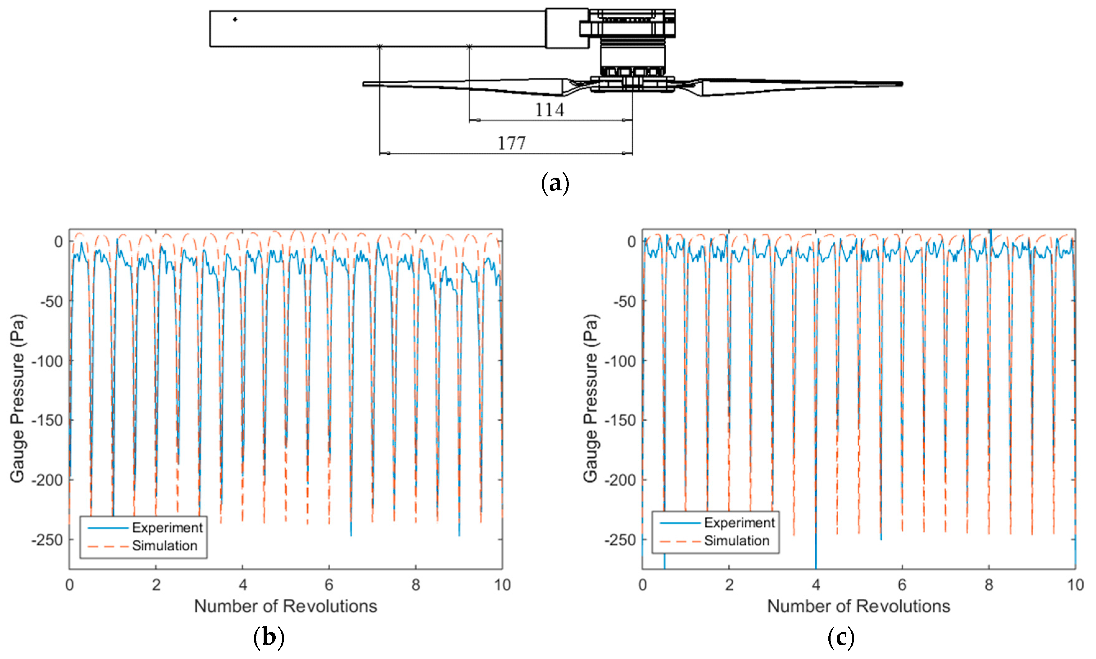
Instead of using the entire UAS for this study, only a single cylindrical airframe and rotor from the DJI S1000 drone were considered.
Figure 1 shows the physical model with the two configurations (i.e., top-mounted and bottom-mounted rotor orientations) employed to investigate the flow and acoustic characteristics. The distance between the rotor and airframe of 27 mm remained constant for the two configurations.
Additional design information about this particular rotor is given in
Figure 2.
Figure 2a shows the rotor pitch angle and non-dimensional chord length distributions in the radial direction. It is noticed that approximately linear taper and twist are employed. Specifically, a taper ratio of 0.42 (ratio of tip chord to root chord) and a linear twist value of −12.5° are used along with a large pitch value of 7.1° at the tip. It can also be seen that a large portion of the rotor (approximately 0.26R) is cutout due to the motor and connection of the blade.
Figure 2b shows the local Reynolds number experienced at different radial locations on the rotor for a rotation rate of 4000 RPM. Based upon [
21,
22], flow transition of airfoils tends to occur in the Reynolds number range of 50,000 to 70,000 depending on many factors, meaning that the rotor investigated in this study may experience this phenomenon. This is an important Reynolds number regime as laminar separation or laminar separation and reattachment due to transition to turbulent flow can occur, causing degraded performance compared to flows at higher Reynolds numbers.
Figure 2c shows the airfoil sections at the root and tip of the rotor blade, which are the same. The airfoil section used is the Althaus AH-6-40-7. This airfoil has a maximum thickness to chord ratio of 6.9% and maximum camber of 5.5% at 40% chord. The particular rotor described in this section is the only geometry tested, both experimentally and computationally. The experimental and computational approaches are described in the following sections.
4. Numerical Approach
A systematic 3-D numerical simulation was performed in STAR-CCM+ to obtain detailed flow fields including velocity, vorticity, and pressure distributions along with acoustic spectrum results. The computational domain has the same dimensions used for taking PIV measurements. In order to match the boundary conditions used during experimental PIV testing, the boundaries in the simulations were set to be non-slip walls. A pressure outlet condition was used for all boundaries in the acoustic simulations as this strategy mimicked an anechoic environment. A steady Reynolds-averaged Navier–Stokes (RANS) simulation was utilized to yield a fully developed initial flow field for the latter unsteady simulations. The SST (Menter)
k-ω improved delayed detached eddy simulation (IDDES) turbulence model, which combines the features of traditional RANS modeling in the boundary layers and large eddy simulation (LES) modeling in the regions beyond boundary layers, was used in this study [
24,
25]. In the IDDES model, the dissipation term,
ω, in the transport equation for turbulent kinetic energy is substituted for
defined as [
25]
where
is a
k-ω model coefficient and
is the free-shear modification factor.
is the hybrid length scale and is defined as
where
is the blending function;
is the turbulent length scale;
is a modified version of the equation for
;
is a model coefficient;
is the mesh length scale which is dependent on the resolution of the cells in the computational domain. This particular turbulence model was used due to the fact that it is a higher fidelity approach compared to the RANS method. Furthermore, with the turbulent structures being modeled more accurately, the accuracy of acoustic results is improved since much of the unsteady loading and noise is caused by turbulent flow structures. It is further acknowledged that a RANS/LES hybrid approach mitigates the problem of artificially large eddy viscosity, a potential issue of the RANS only model. This issue can lead to inaccurate modeling of vortical structures and boundary layers on or in close proximity to the rotor [
14].
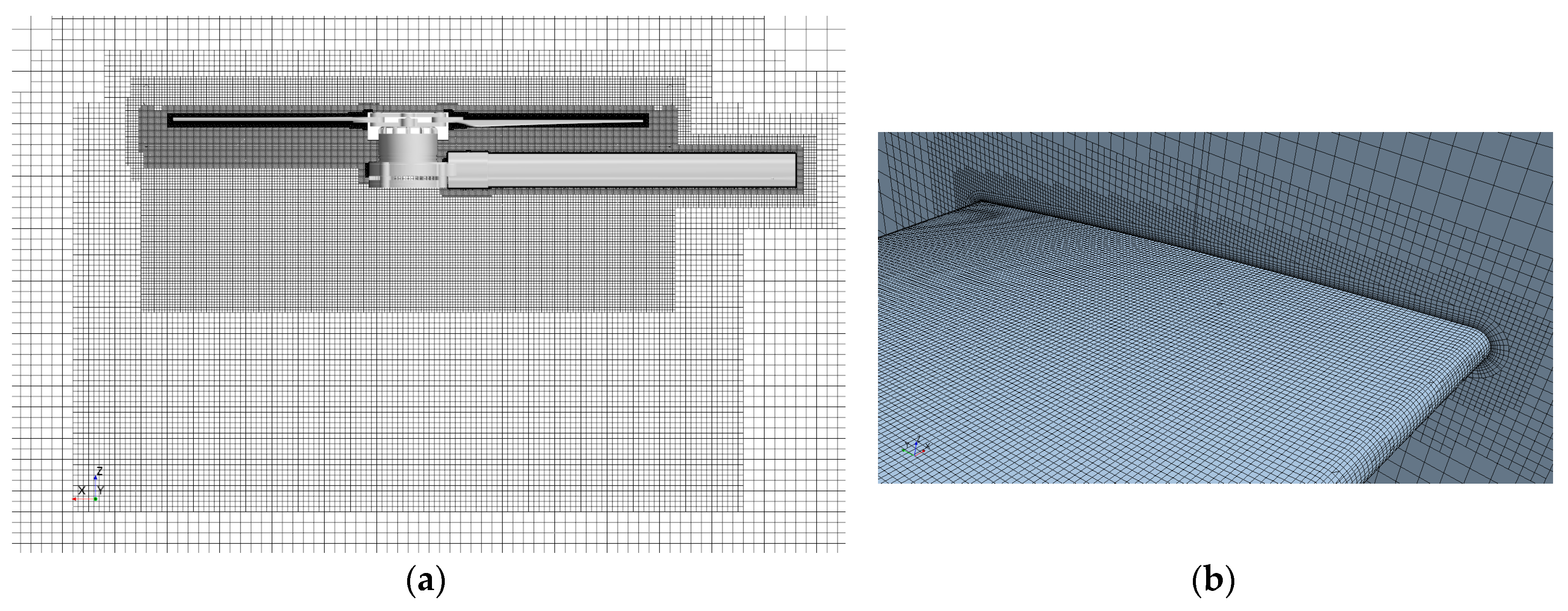
In order to mimic rotor motion, the computational domain was split into a rotating region, which encapsulates the rotor, and a stationary region. During the unsteady simulation, the rotating region moved and a sliding mesh technique was used to update the mesh at the interfaces where the rotating and stationary regions contact. A large time step was used for the first several revolutions and then the time step was gradually decreased to achieve better convergence and more accurate results. The final time step employed in the unsteady simulation equals to a 1° azimuthal increment of the rotor blade. A mesh sensitivity study was also conducted to examine if the employed mesh is sufficient to resolve the dominant flow features and to ensure mesh independence. A mesh with 15.3 million trimmed (hexahedral) cells was used in the current study. The meshes near the rotor and airframe were refined accordingly to achieve high-resolution in these regions. Consequently, the wall y+ values on the rotor blade surfaces and airframe were found to be 1 or less. The mesh was also refined in the wake to resolve convecting flow structures more accurately.
Figure 6 illustrates the mesh generated around the rotor, and in the wake region for the top-mounted configuration.
When a stable unsteady result was attained, the Ffowcs Williams-Hawkings (FW-H) formulation was employed to calculate the far-field acoustic pressure based on the near-field sources, such as the rotor and airframe. The FW-H method is widely known as an effective methodology to predict the sound generated from rigid bodies in arbitrary motion and can be derived directly by reformatting the Navier–Stokes equations into the form of the acoustic wave equation [
26]. The thickness and loading terms of the FW-H formulation were considered while the quadrupole term was omitted due to the need for extremely high mesh resolution to calculate this particular source accurately. As discussed in the introduction, this source, which calculates some of the broadband noise, is typically calculated using other means. The thickness term includes noise caused by displaced fluid as the rotor rotates while the loading term calculates noise caused by the pressure distribution on the rotor and airframe. The loading term includes noise caused by both steady and unsteady loading. The thickness and loading terms are represented by monopole and dipole sources, respectively, and are defined by Equations (4) and (5) [
27]. This specific mathematical representation of the two sources is called Farassat’s 1A formulation.
In Equations (4) and (5), and are the acoustic pressure fluctuations from the mean for the thickness and loading terms, respectively. is the density of the fluid; r is the distance between the source and the receiver; is the Mach number of the source in the direction of the receiver; is the normal velocity of the source surface; M is the Mach number vector of the source; dS is an element of the rotor blade surface; is the fluid’s speed of sound; is the local force that acts on the fluid in the direction towards the receiver; is the local force that acts on the fluid in the direction towards the local Mach number vector of the source. It should be noted that the subscripted quantities in these equations are the inner products of a vector and a unit vector. A variable with a dot above it signifies a time derivative.
6. Conclusions
The purpose of this study was to investigate the similarities and differences in aerodynamic and acoustic characteristics for two different configurations (top-mounted and bottom-mounted) of a small UAS/UAV rotor and airframe. A detailed investigation including PIV, pressure, and acoustic measurements, and comprehensive simulations were applied to compare the two configurations.
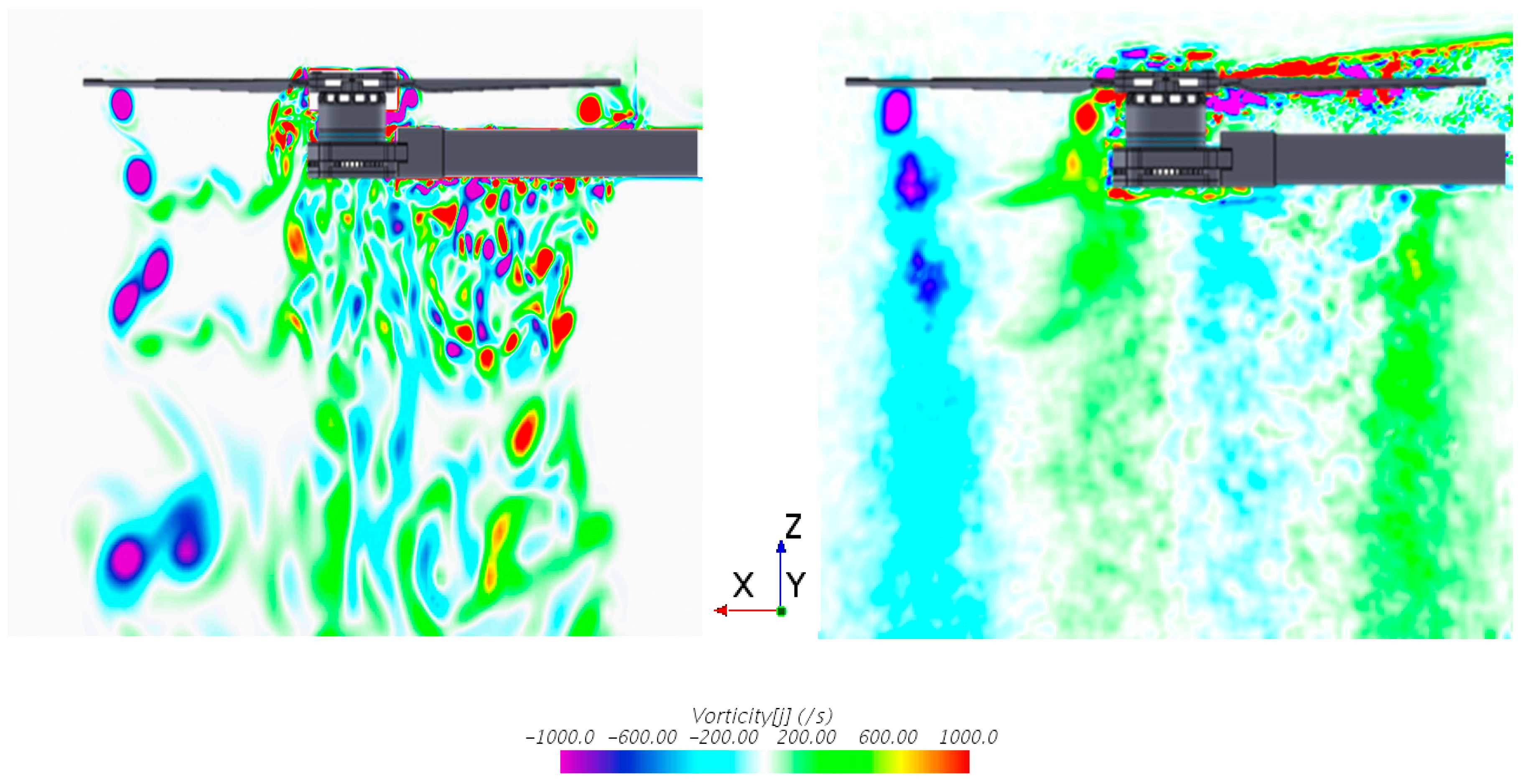
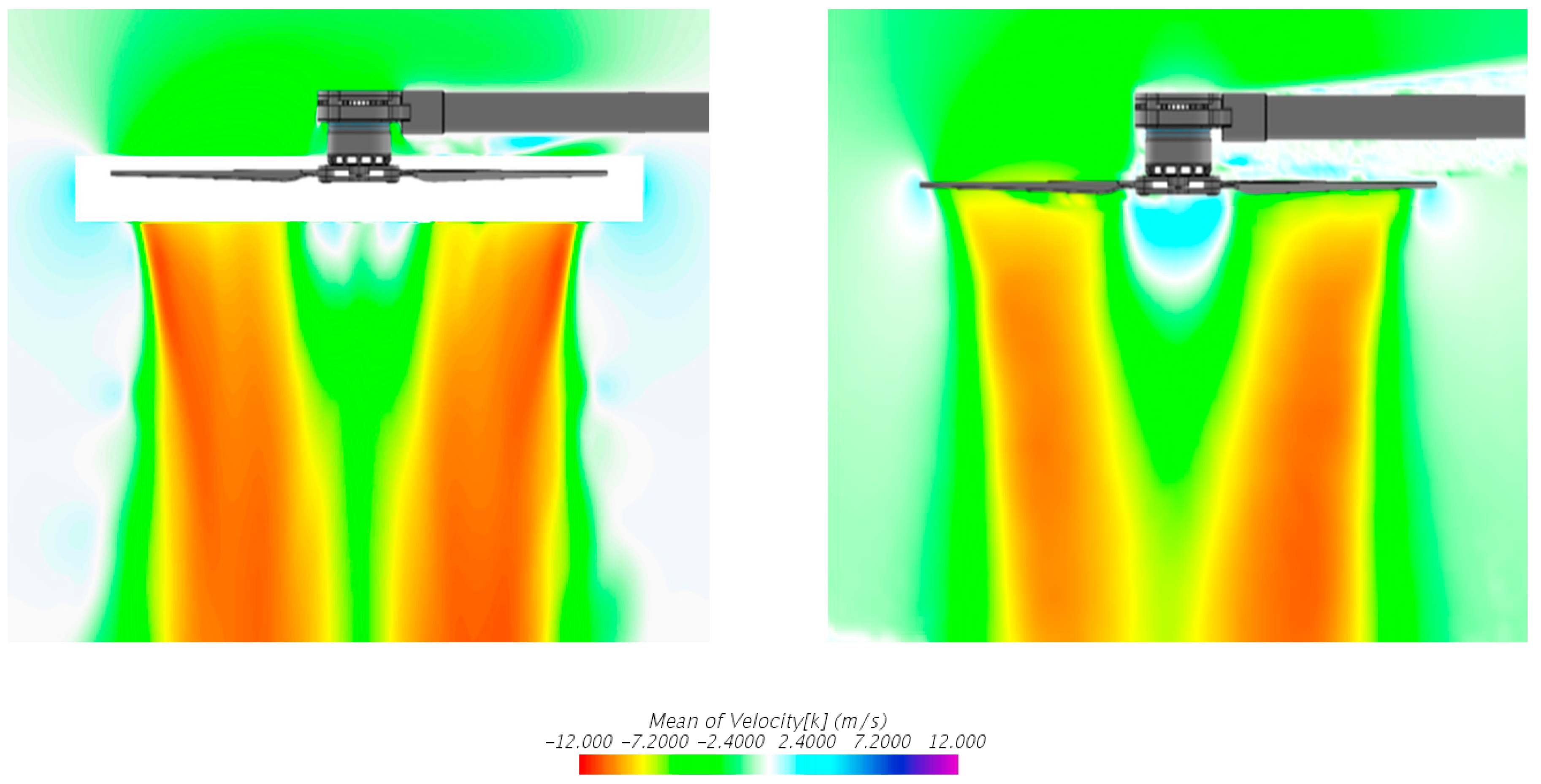
In summary, it was found that the tip vortices were stronger and rotated in the opposite direction compared to those shed by the trailing edge. Moreover, these vortical structures were well resolved by the simulation, showing similar trends with the experiment such as structure, magnitude, and dissipation as they convected farther axially into the wake. The wake sheets were found to be flat and the axial velocity fields are fairly uniform in magnitude, suggesting uniform aerodynamic loads acting on the rotor blades. It is observed that vortical structures tend to be reflected or generated in the upward direction off of the airframe into the rotor plane for the top-mounted configuration. For the bottom-mounted configuration, vortical structures tend to be sucked into the rotor plane due to the proximity airframe. It is also noted for the top-mounted rotor that the airframe significantly obstructs the flow, causing the magnitude of the velocity to be slower in portions of the wake affected by the airframe.
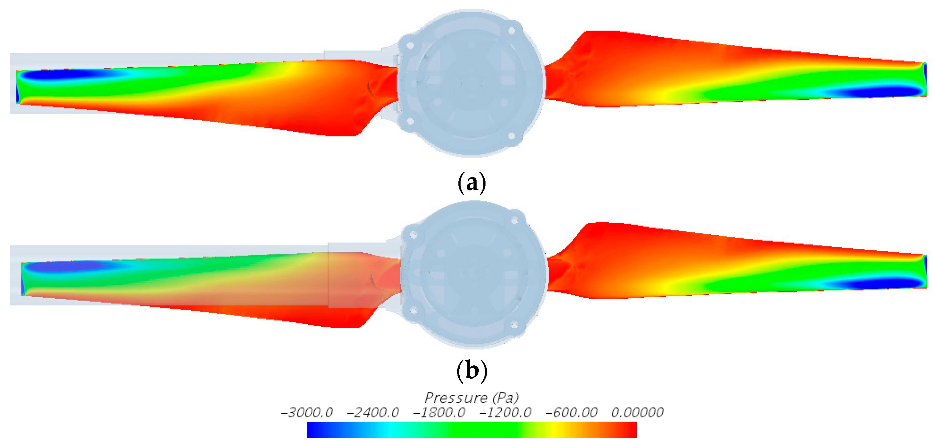
Pressure contours of the rotor showed that the airframe had little to no impact on the pressure distribution and magnitude on the rotor blades. The contours also implied that little to no thrust is produced by the quarter inner section of the rotor and that the flow detaches on the top portion of the rotor at this location. The pressure contours and measurements from the airframe showed that the top-mounted configuration produced regions of negative and positive pressure while the bottom-mounted configuration only produced negative pressures. Positive pressures occurred for the top-mounted rotor due to flow impingement while negative pressures occurred due to air flowing past the airframe and close proximity tip vortices. The airframe for the bottom-mounted configuration only experienced negative pressures due to the proximity of the suction side of the rotor.
From the acoustic results, it was observed that the bottom-mounted configuration produced more noise at the in-plane receiver due to an increase in the amplitude of BPF harmonics and high frequency noise. For the normal receiver, it was seen that the bottom-mounted configuration produced slightly more broadband noise in the low to mid frequencies. Similarly, this configuration also produced slightly greater tonal and broadband noise in the high frequency range. It can be concluded that these slight increases in noise, which can be seen across the entire spectrum of frequencies, for the bottom-mounted configuration can be attributed to the distorted inflow caused by the airframe. The airframe, in this configuration, not only produces large periodic turbulent structures which can cause tonal noise, but can also cause smaller turbulent structures to continually impact the rotor, resulting in broadband noise. Overall, the simulation was able to predict tonal noise up to approximately 1500 Hz for both configurations and receiver locations, but was unable to accurately predict broadband and high frequency noise partially due to the lack of a broadband noise model in the FW-H formulation. The lack of accuracy in the high frequency range may also be due to the computational model, which does not consider noise from the motor, mechanical vibrations, ESC, and other sources.

 and
and 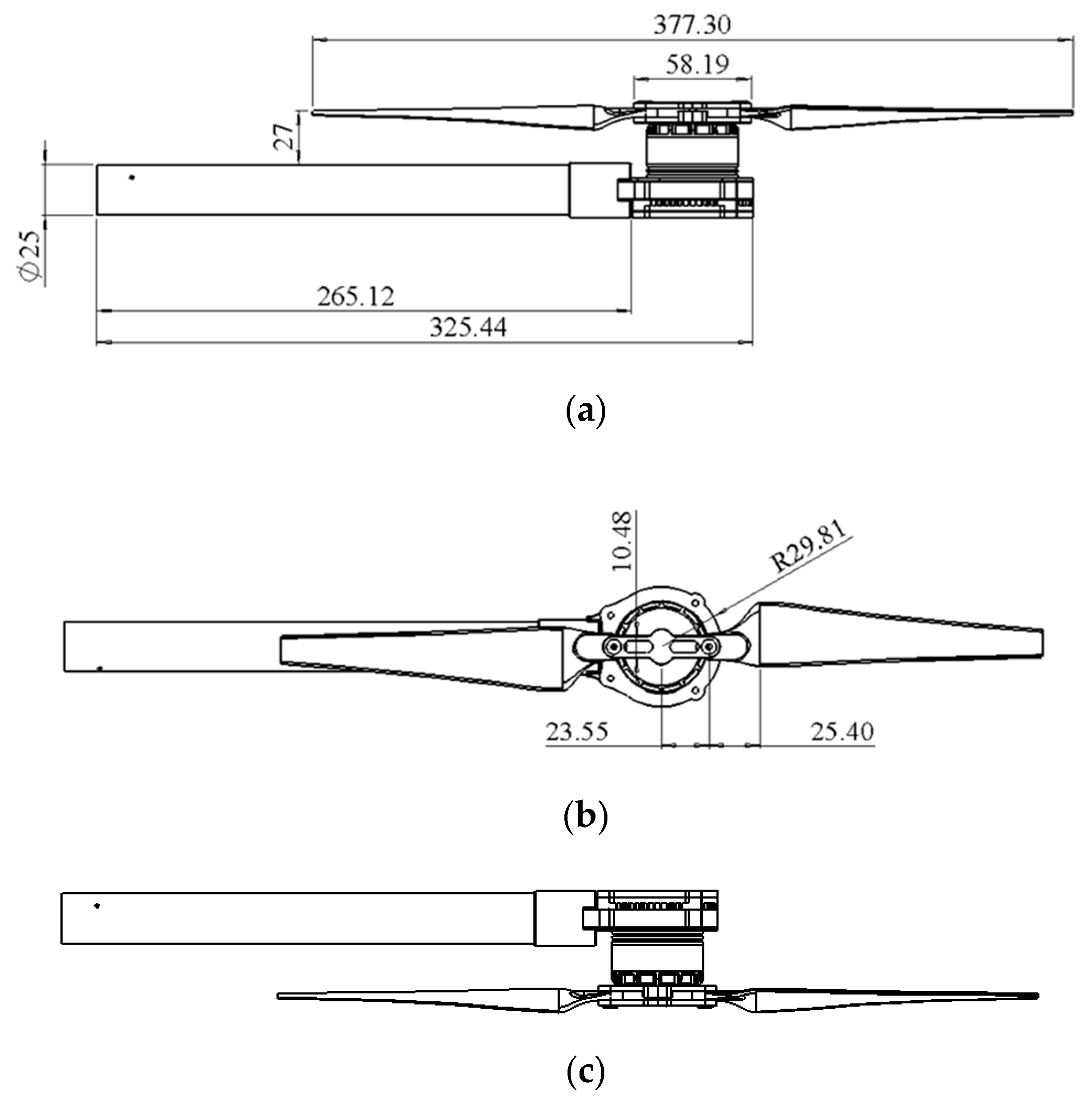


