Using Unmanned Aerial Systems (UAS) and Object-Based Image Analysis (OBIA) for Measuring Plant-Soil Feedback Effects on Crop Productivity


Abstract
:1. Introduction
2. Materials and Methods
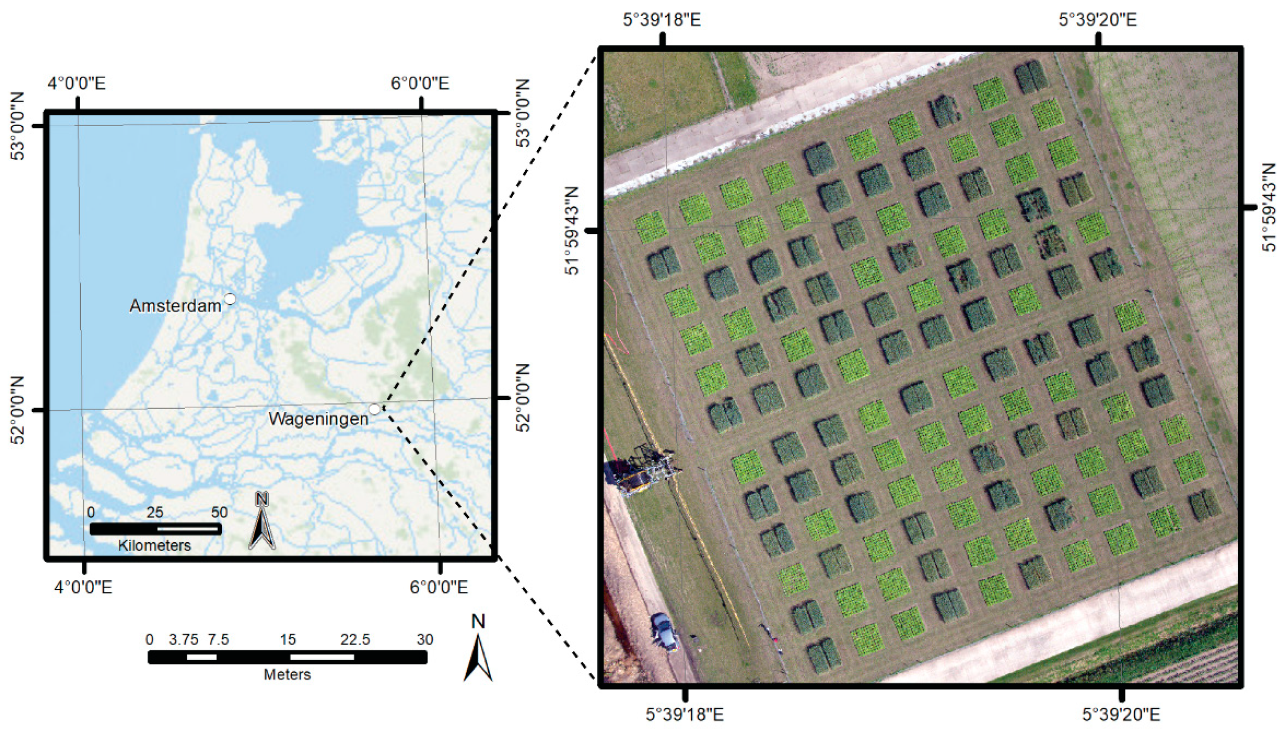
2.1. Study Area
2.2. Data
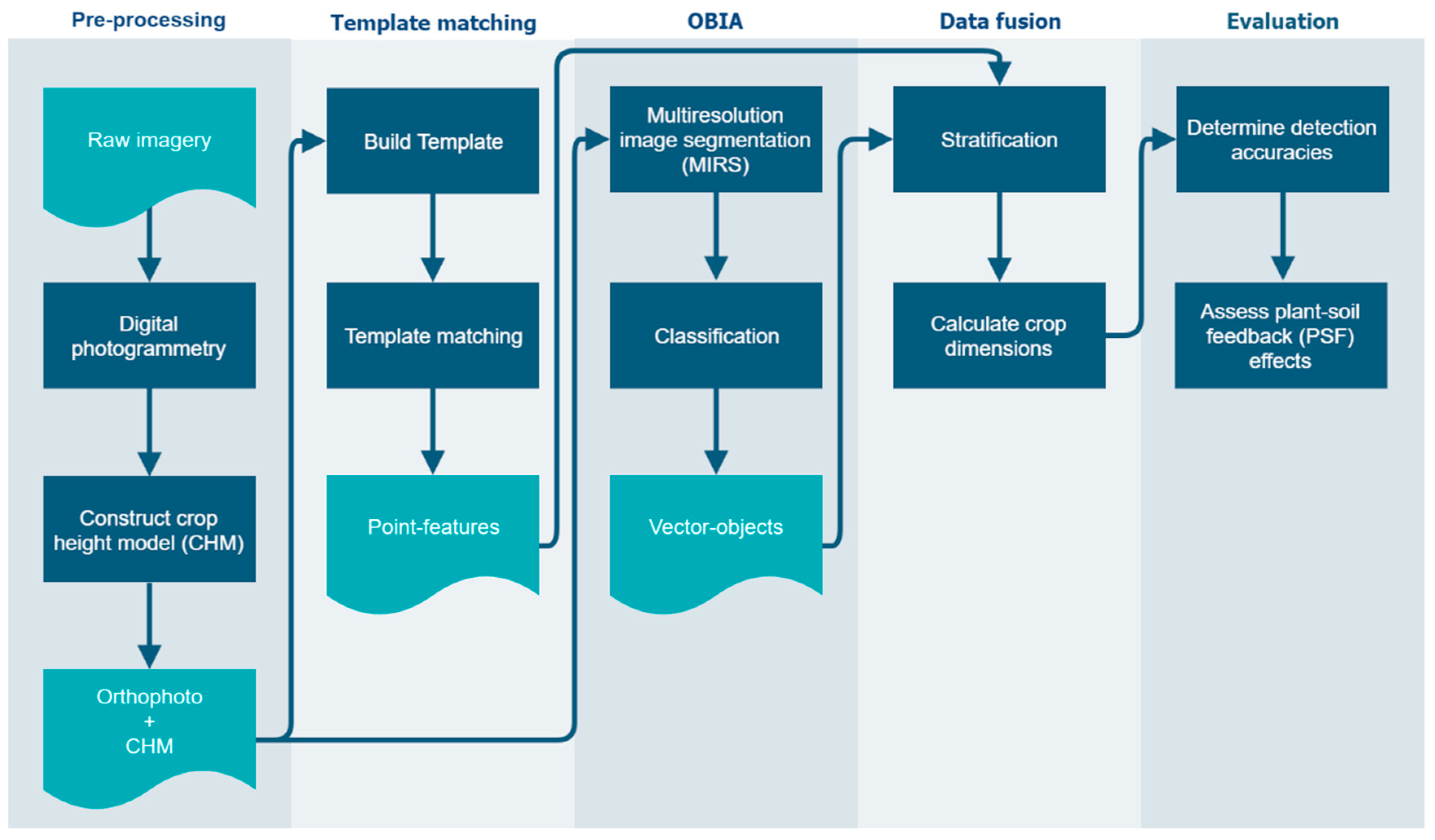
2.3. Processing and Analysis
2.3.1. Pre-Processing
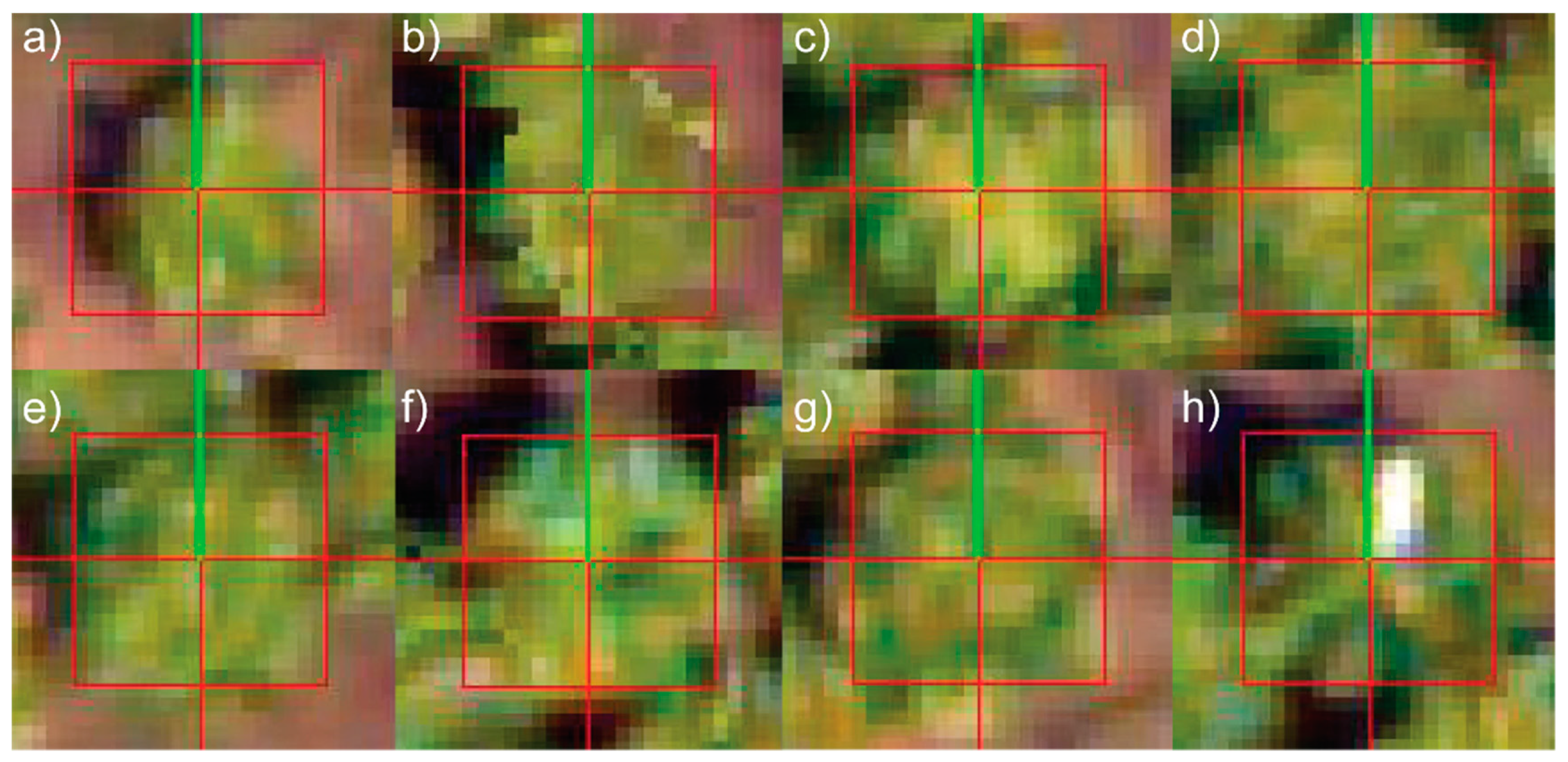
2.3.2. Template Matching
2.3.3. Object-Based Image Analysis
2.3.4. Data Fusion
2.3.5. Evaluation
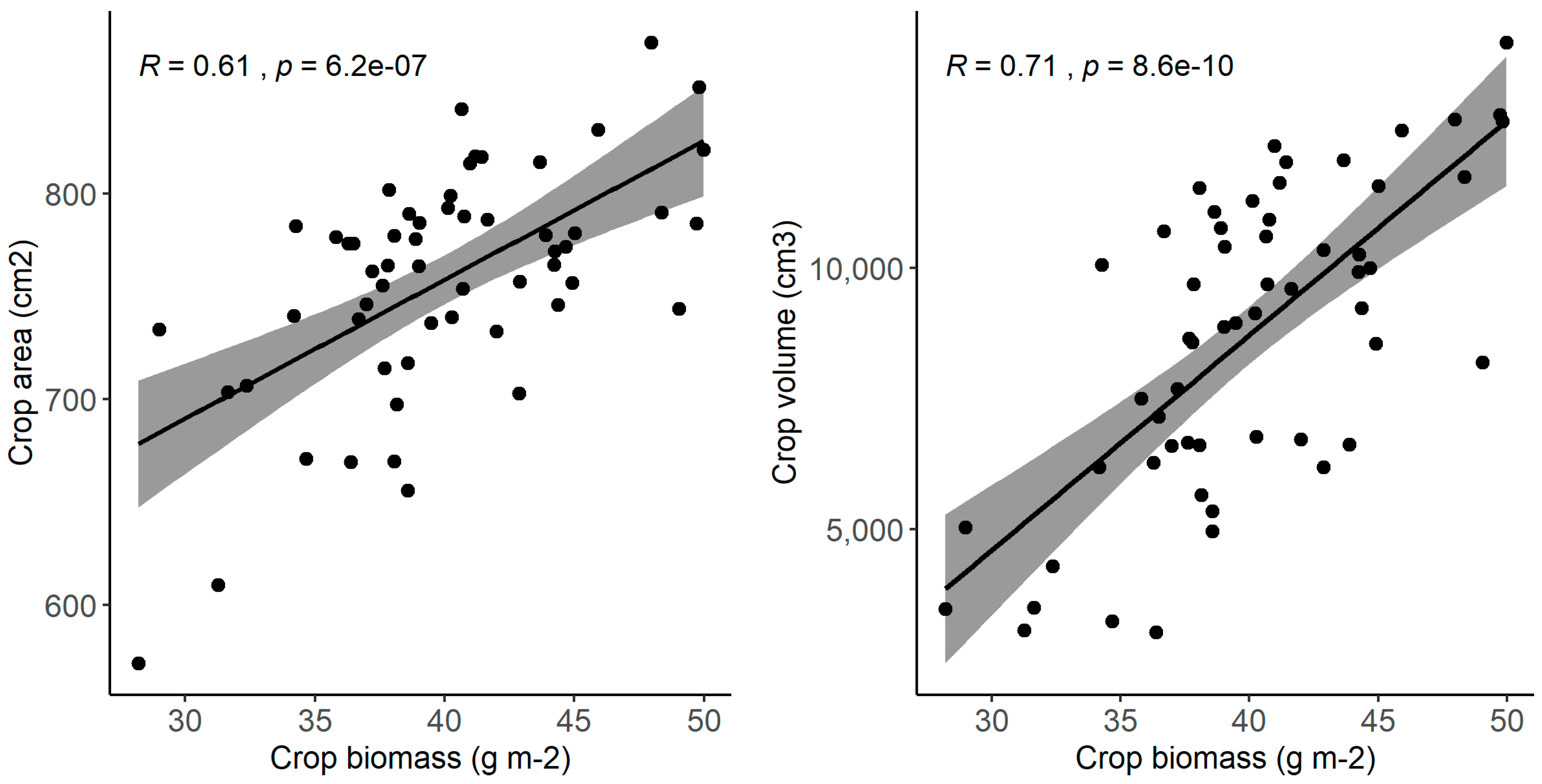
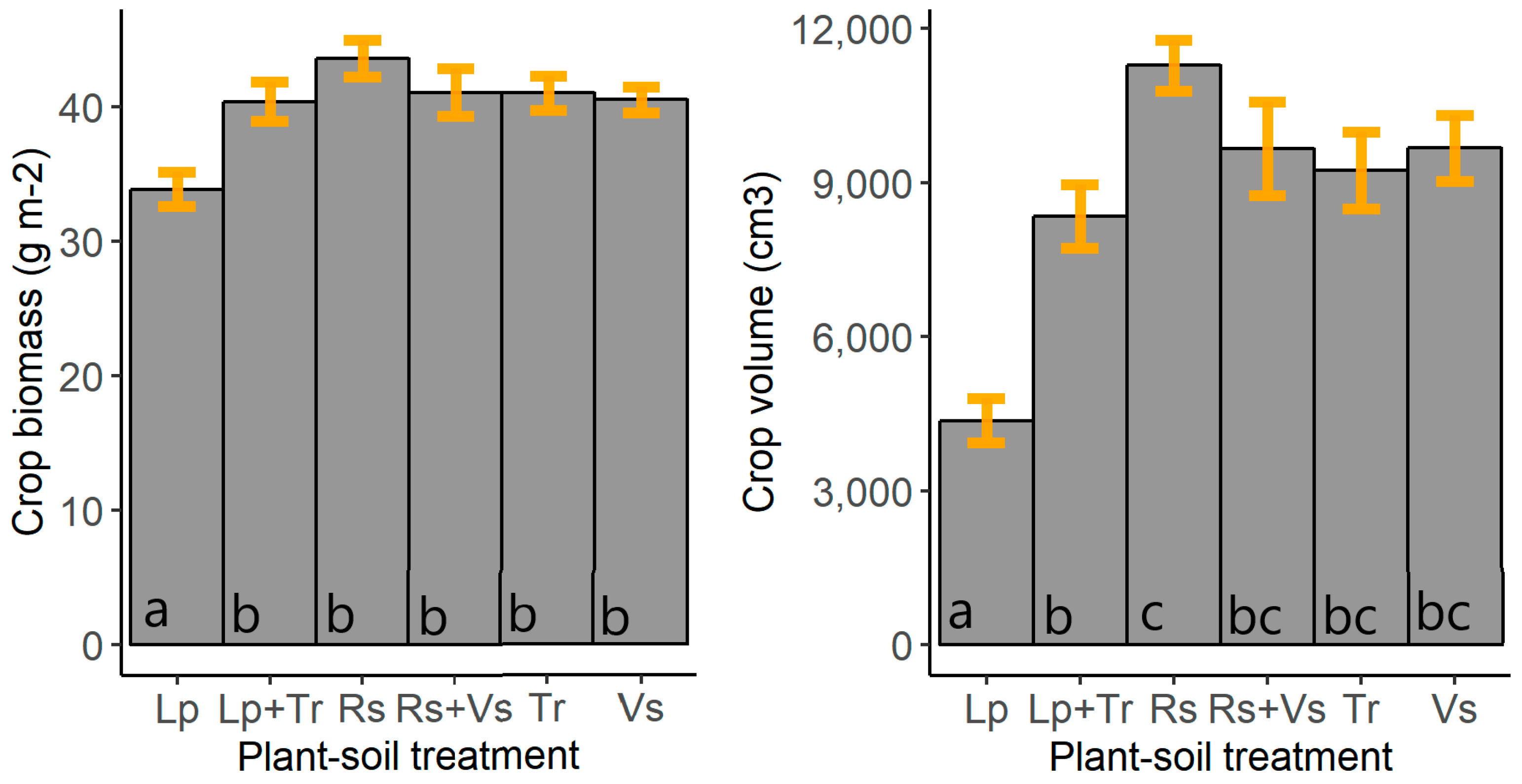
3. Results
4. Discussion
4.1. Object-Based Image Analysis
4.2. Crop Height Model
4.3. Plant-Soil Feedback
4.4. Scalability
5. Conclusions
Author Contributions
Funding
Acknowledgments
Conflicts of Interest
References
- Cortois, R.; Schröder-Georgi, T.; Weigelt, A.; van der Putten, W.; De Deyn, G. Plant–soil feedbacks: Role of plant functional group and plant traits. J. Ecol. 2016, 104, 1608–1617. [Google Scholar] [CrossRef]
- Barel, J.; Kuyper, T.; de Boer, W.; Douma, J.; De Deyn, G. Legacy effects of diversity in space and time driven by winter cover crop biomass and nitrogen concentration. J. Appl. Ecol. 2018, 55, 299–310. [Google Scholar] [CrossRef]
- Pernilla Brinkman, E.; Van der Putten, W.H.; Bakker, E.; Verhoeven, K.J.F. Plant-soil feedback: Experimental approaches, statistical analyses and ecological interpretations. J. Ecol. 2010, 98, 1063–1073. [Google Scholar] [CrossRef]
- van der Putten, W.; Bardgett, R.; Bever, J.; Bezemer, T.; Casper, B.; Fukami, T.; Kardol, P.; Klironomos, J.; Kulmatiski, A.; Schweitzer, J.; et al. Plant-soil feedbacks: The past, the present and future challenges. J. Ecol. 2013, 101, 265–276. [Google Scholar] [CrossRef]
- Dias, T.; Dukes, A.; Antunes, P.M. Accounting for soil biotic effects on soil health and crop productivity in the design of crop rotations. J. Sci. Food Agric. 2015, 95, 447–454. [Google Scholar] [CrossRef]
- Nebiker, S.; Annen, A.; Scherrer, M.; Oesch, D. A Light-weight Multispectral Sensor for Micro UAV—Opportunities for Very High Resolution Airborne Remote Sensing. Int. Arch. Photogramm. Remote Sens. Spat. Inf. Sci. 2008, 37, 1193–1200. [Google Scholar]
- Kulmatiski, A.; Kardol, P. Getting Plant—Soil Feedbacks out of the Greenhouse: Experimental and Conceptual Approaches. In Progress in Botany; Springer: Berlin/Heidelberg, Germany, 2008; Volume 69, pp. 449–472. [Google Scholar]
- van der Meij, B.; Kooistra, L.; Suomalainen, J.; Barel, J.; De Deyn, G. Remote sensing of plant trait responses to field-based plant–soil feedback using UAV-based optical sensors. Biogeosciences 2017, 14, 733–749. [Google Scholar] [CrossRef]
- Anderson, K.; Gaston, K.J. Lightweight unmanned aerial vehicles will revolutionize spatial ecology. Front. Ecol. Environ. 2013, 11, 138–146. [Google Scholar] [CrossRef] [Green Version]
- Dixon, J.; McCann, M. Precision Agriculture in the 21st Century: Geospatial and Information Technologies in Crop Management; The National Academies Press: Washington, DC, USA, 1997. [Google Scholar]
- Mulla, D.J. Twenty five years of remote sensing in precision agriculture: Key advances and remaining knowledge gaps. Biosyst. Eng. 2013, 114, 358–371. [Google Scholar] [CrossRef]
- Tian, L. Development of a sensor-based precision herbicide application system. Comput. Electron. Agric. 2002, 36, 133–149. [Google Scholar] [CrossRef]
- Feng, Q.; Liu, J.; Gong, J. UAV Remote Sensing for Urban Vegetation Mapping Using Random Forest and Texture Analysis. Remote Sens. 2015, 7, 1074–1094. [Google Scholar] [CrossRef] [Green Version]
- Andújar, D.; Ribeiro, A.; Fernández-Quintanilla, C.; Dorado, J. Using depth cameras to extract structural parameters to assess the growth state and yield of cauliflower crops. Comput. Electron. Agric. 2016, 122, 67–73. [Google Scholar] [CrossRef]
- Faye, E.; Rebaudo, F.; Yánez-Cajo, D.; Cauvy-Fraunié, S.; Dangles, O. A toolbox for studying thermal heterogeneity across spatial scales: From unmanned aerial vehicle imagery to landscape metrics. Methods Ecol. Evol. 2016, 7, 437–446. [Google Scholar] [CrossRef]
- Guo, Q.; Wu, F.; Pang, S.; Zhao, X.; Chen, L.; Liu, J.; Xue, B.; Xu, G.; Li, L.; Jing, H.; et al. Crop 3D—A LiDAR based platform for 3D high-throughput crop phenotyping. Sci. China Life Sci. 2018, 61, 328–339. [Google Scholar] [CrossRef] [PubMed]
- Li, L.; Zhang, Q.; Huang, D. A Review of Imaging Techniques for Plant Phenotyping. Sensors 2014, 14, 20078–20111. [Google Scholar] [CrossRef] [PubMed]
- Christiansen, M.P.; Laursen, M.S.; Jørgensen, R.N.; Skovsen, S.; Gislum, R. Designing and Testing a UAV Mapping System for Agricultural Field Surveying. Sensors 2017, 17, 2703. [Google Scholar] [CrossRef] [PubMed]
- Schirrmann, M.; Giebel, A.; Gleiniger, F.; Pflanz, M.; Lentschke, J.; Dammer, K. Monitoring Agronomic Parameters of Winter Wheat Crops with Low-Cost UAV Imagery. Remote Sens. 2016, 8, 706. [Google Scholar] [CrossRef]
- Mathews, A.; Jensen, J.; Mathews, A.J.; Jensen, J.L.R. Visualizing and Quantifying Vineyard Canopy LAI Using an Unmanned Aerial Vehicle (UAV) Collected High Density Structure from Motion Point Cloud. Remote Sens. 2013, 5, 2164–2183. [Google Scholar] [CrossRef] [Green Version]
- Ballesteros, R.; Ortega, J.F.; Hernandez, D.; Moreno, M.A. Onion biomass monitoring using UAV-based RGB imaging. Precis. Agric. 2018, 19, 840–857. [Google Scholar] [CrossRef]
- White, J.C.; Wulder, M.A.; Vastaranta, M.; Coops, N.C.; Pitt, D.; Woods, M. The utility of image-based point clouds for forest inventory: A comparison with airborne laser scanning. Forests 2013, 4, 518–536. [Google Scholar] [CrossRef]
- Colomina, I.; Molina, P. Unmanned aerial systems for photogrammetry and remote sensing: A review. ISPRS J. Photogramm. Remote Sens. 2014, 92, 79–97. [Google Scholar] [CrossRef] [Green Version]
- Jóźków, G.; Toth, C.K.; Grejner-Brzezinska, D. UAS Topographic Mapping with Volodyne LiDAR Sensor. ISPRS Ann. Photogramm. Remote Sens. Spat. Inf. Sci. 2016, III, 201–208. [Google Scholar] [CrossRef]
- Cheng, G.; Han, J. A survey on object detection in optical remote sensing images. ISPRS J. Photogramm. Remote Sens. 2016, 117, 11–28. [Google Scholar] [CrossRef] [Green Version]
- Tiede, D.; Krafft, P.; Füreder, P.; Lang, S. Stratified template matching to support refugee camp analysis in OBIA workflows. Remote Sens. 2017, 9, 326. [Google Scholar] [CrossRef]
- Kalantar, B.; Mansor, S.B.; Zulhaidi, H.; Shafri, M.; Halin, A.A. Integration of template matching and object-based image analysis for semi-automatic oil palm tree counting in UAV images. In Proceedings of the 37th Asian Conference on Remote Sensing, Colombo, Sri Lanka, 17–21 October 2016. [Google Scholar]
- Blaschke, T. Object based image analysis for remote sensing. ISPRS J. Photogramm. Remote Sens. 2010, 65, 2–16. [Google Scholar] [CrossRef] [Green Version]
- Hay, G.; Castilla, G. Geographic Object-Based Image Analysis (GEOBIA): A new name for a new discipline. Object-Based Image Anal. 2008, 75–89. [Google Scholar]
- Benz, U.; Hofmann, P.; Willhauck, G.; Lingenfelder, I.; Heynen, M. Multi-resolution, object-oriented fuzzy analysis of remote sensing data for GIS-ready information. ISPRS J. Photogramm. Remote Sens. 2004, 58, 239–258. [Google Scholar] [CrossRef]
- Castillejo-González, I.; López-Granados, F.; García-Ferrer, A.; Peña, J.; Jurado-Expósito, M.; de la Orden, M.; González-Audicana, M. Object- and pixel-based analysis for mapping crops and their agro-environmental associated measures using QuickBird imagery. Comput. Electron. Agric. 2009, 68, 207–215. [Google Scholar] [CrossRef]
- Yu, Q.; Gong, P.; Clinton, N.; Biging, G.; Kelly, M.; Schirokauer, D. Object-based Detailed Vegetation Classification with Airborne High Spatial Resolution Remote Sensing Imagery. Photogramm. Eng. Remote Sens. 2006, 72, 799–811. [Google Scholar] [CrossRef] [Green Version]
- Yan, G.; Mas, J.; Maathuis, B.; Xiangmin, Z.; Dijk, P. van Comparison of pixel-based and object-oriented image classification approaches—A case study in a coal fire area, Wuda, Inner Mongolia, China. Int. J. Remote Sens. 2006, 27, 4039–4055. [Google Scholar] [CrossRef]
- Platt, R.; Rapoza, L. An Evaluation of an Object-Oriented Paradigm for Land Use/Land Cover Classification. Prof. Geogr. 2008, 60, 87–100. [Google Scholar] [CrossRef]
- Wang, L.; Sousa, W.; Gong, P. Integration of object-based and pixel-based classification for mapping mangroves with IKONOS imagery. Int. J. Remote Sens. 2004, 25, 5655–5668. [Google Scholar] [CrossRef]
- Peña-Barragán, J.; Gutiérrez, P.; Hervás-Martínez, C.; Six, J.; Plant, R.E.; López-Granados, F. Object-Based Image Classification of Summer Crops with Machine Learning Methods. Remote Sens. 2014, 6, 5019–5041. [Google Scholar] [CrossRef] [Green Version]
- Peña-Barragán, J.; Kelly, M.; de Castro, A.I.; López-Granados, F. Object-Based Approach for Crop Row Characterization in Uav Images for Site-Specific Weed Management. In Proceedings of the 4th Geographic Object-Based Image Analysis (GEOBIA) Conference, Rio de Janeiro, Brazil, 7–9 May 2012; pp. 426–430. [Google Scholar]
- Suomalainen, J.; Anders, N.; Iqbal, S.; Roerink, G.; Franke, J.; Wenting, P.; Hünniger, D.; Bartholomeus, H.; Becker, R.; Kooistra, L. A Lightweight Hyperspectral Mapping System and Photogrammetric Processing Chain for Unmanned Aerial Vehicles. Remote Sens. 2014, 6, 11013–11030. [Google Scholar] [CrossRef] [Green Version]
- Jebara, T.; Azarbayejani, A.; Pentland, A. 3D structure from 2D motion. IEEE Signal Process. Mag. 1999, 16, 66–84. [Google Scholar] [CrossRef]
- Agisoft LLC. Agisoft PhotoScan Professional Edition 2018; Agisoft LLC: Saint Petersburg, Russia, 2018. [Google Scholar]
- van der Meij, B. Measuring the Legacy of Plants and plant Traits Using UAV-Based Optical Sensors. Masters’ Thesis, Utrecht University, Utrecht, The Netherlands, 2016. [Google Scholar]
- Boissonnat, J.D.; Gazais, F. Smooth surface reconstruction via natural neighbour interpolation of distance functions. Comput. Geom. Theory Appl. 2002, 22, 185–203. [Google Scholar] [CrossRef] [Green Version]
- Lewis, J.P. Fast Template Matching Template Matching by Cross Correlation 2 Normalized Cross Correlation Normalized Cross Correlation in the Transform Domain. Pattern Recognit. 1995, 10, 120–123. [Google Scholar]
- Flanders, D.; Hall-Beyer, M.; Pereverzoff, J. Preliminary evaluation of eCognition object-based software for cut block delineation and feature extraction. Can. J. Remote Sens. 2003, 29, 441–452. [Google Scholar] [CrossRef]
- Reis, M.S.; de Oliveira, M.A.F.; Korting, T.S.; Pantaleao, E.; Sant’Anna, S.J.S.; Dutra, L.V.; Lu, D. Image segmentation algorithms comparison. In Proceedings of the 2015 IEEE International Geoscience and Remote Sensing Symposium (IGARSS), Milan, Italy, 26–31 July 2015; pp. 4340–4343. [Google Scholar]
- Nuijten, R.J.G. Developing OBIA Methods for Measuring Plant Traits and the Legacy of Crops Using VHR UAV-Based Optical Sensors. Masters’ Thesis, Universiteit Utrecht, Utrecht, The Netherlands, 2018. [Google Scholar]
- Hunt, E.R.; Daughtry, C.S.T.; Eitel, J.U.H.; Long, D.S. Remote Sensing Leaf Chlorophyll Content Using a Visible Band Index. Agron. J. 2011, 103, 1090. [Google Scholar] [CrossRef]
- Mckinnon, T.; Hoff, P. Comparing RGB-Based Vegetation Indices with NDVI for Drone Based Agricultural Sensing; Agribotix LLC: Saint Petersburg, Russia, 2017; pp. 1–8. [Google Scholar]
- Pouliot, D.A.; King, D.J.; Bell, F.W.; Pitt, D.G. Automated tree crown detection and delineation in high-resolution digital camera imagery of coniferous forest regeneration. Remote Sens. Environ. 2002, 82, 322–334. [Google Scholar] [CrossRef]
- Soper, H.E.; Young, A.W.; Cave, B.M.; Lee, A.; Pearson, K. On the Distribution of the correlation coefficient in small samples. Biometrika 1932, 24, 382–403. [Google Scholar]
- Tukey, J.W. Comparing Individual Means in the Analysis of Variance. Biometrics 1949, 5, 99. [Google Scholar] [CrossRef] [PubMed]
- Ruxton, G.D.; Beauchamp, G. Time for some a priori thinking about post hoc testing. Behav. Ecol. 2008, 19, 690–693. [Google Scholar] [CrossRef] [Green Version]
- Goodbody, T.R.H.; Coops, N.C.; Hermosilla, T.; Tompalski, P.; Pelletier, G. Vegetation Phenology Driving Error Variation in Digital Aerial Photogrammetrically Derived Terrain Models. Remote Sens. 2018, 10, 1554. [Google Scholar] [CrossRef]
- Turner, D.; Lucieer, A.; Watson, C.; Turner, D.; Lucieer, A.; Watson, C. An Automated Technique for Generating Georectified Mosaics from Ultra-High Resolution Unmanned Aerial Vehicle (UAV) Imagery, Based on Structure from Motion (SfM) Point Clouds. Remote Sens. 2012, 4, 1392–1410. [Google Scholar] [CrossRef] [Green Version]
- Ouédraogo, M.; Degré, A.; Debouche, C.; Lisein, J. The evaluation of unmanned aerial system-based photogrammetry and terrestrial laser scanning to generate DEMs of agricultural watersheds. Geomorphology 2014, 214, 339–355. [Google Scholar] [CrossRef]
- Tian, Y.C.; Yao, X.; Yang, J.; Cao, W.X.; Hannaway, D.B.; Zhu, Y. Assessing newly developed and published vegetation indices for estimating rice leaf nitrogen concentration with ground- and space-based hyperspectral reflectance. Field Crops Res. 2010, 120, 299–310. [Google Scholar] [CrossRef]
- Ciganda, V.; Gitelson, A.; Schepers, J. Non-destructive determination of maize leaf and canopy chlorophyll content. J. Plant Physiol. 2009, 166, 157–167. [Google Scholar] [CrossRef] [Green Version]


| Field Characteristic | Data |
|---|---|
| Crop count | 5930 |
| Plot count | 60 |
| Plot dimensions | 3 × 3 m2 |
| Crop species | Endive |
| Cover crop species | Radish (Raphanus sativus; Rs), perennial ryegrass (Lolium perenne; Lp), white clover (Trifolium repens; Tr), and common vetch (Vicia sativa; Vs) |
| Cover crop treatments | Monocultures: Rs, Lp, Tr, and Vs; mixtures: Rs+Vs and Lp+Tr; fallow |
| Metric | OBIA | Stratified TM |
|---|---|---|
| True positives | 429.3 m2 | 5,921 crops |
| False positives | 14.2 m2 | 1 crops |
| False negatives | 56.9 m2 | 9 crops |
| Detection rate | 88.3% | 99.9% |
| Accuracy index | 85.4% | 99.8% |
© 2019 by the authors. Licensee MDPI, Basel, Switzerland. This article is an open access article distributed under the terms and conditions of the Creative Commons Attribution (CC BY) license (http://creativecommons.org/licenses/by/4.0/).
Share and Cite
Nuijten, R.J.G.; Kooistra, L.; De Deyn, G.B. Using Unmanned Aerial Systems (UAS) and Object-Based Image Analysis (OBIA) for Measuring Plant-Soil Feedback Effects on Crop Productivity. Drones 2019, 3, 54. https://doi.org/10.3390/drones3030054
Nuijten RJG, Kooistra L, De Deyn GB. Using Unmanned Aerial Systems (UAS) and Object-Based Image Analysis (OBIA) for Measuring Plant-Soil Feedback Effects on Crop Productivity. Drones. 2019; 3(3):54. https://doi.org/10.3390/drones3030054
Chicago/Turabian StyleNuijten, Rik J. G., Lammert Kooistra, and Gerlinde B. De Deyn. 2019. "Using Unmanned Aerial Systems (UAS) and Object-Based Image Analysis (OBIA) for Measuring Plant-Soil Feedback Effects on Crop Productivity" Drones 3, no. 3: 54. https://doi.org/10.3390/drones3030054
APA StyleNuijten, R. J. G., Kooistra, L., & De Deyn, G. B. (2019). Using Unmanned Aerial Systems (UAS) and Object-Based Image Analysis (OBIA) for Measuring Plant-Soil Feedback Effects on Crop Productivity. Drones, 3(3), 54. https://doi.org/10.3390/drones3030054