Neural-Network Surrogate Framework for Rapid LCA Impact Screening of Potato Production: Manual Management vs. Drone-Assisted Technification

Highlights

What are the main findings?

• Variable-rate targeting enabled by unmanned aerial vehicles can be assessed at scale by coupling life cycle assessment outputs with artificial neural network surrogate models for rapid multi-impact prediction.
• Across Ecuadorian potato production from 2015 to 2024, the drone-based variable-rate application scenario shows systematic environmental improvements compared with conventional management.

What are the implications of the main findings?

• The approach accelerates unmanned aerial vehicle technology evaluation by transforming life cycle assessment into an efficient predictive tool for scenario planning and optimization.
• A reproducible implementation improves adoption in Global South settings where full-resolution life cycle assessment data collection is challenging.

Abstract

Potato cultivation in the Ecuadorian Andes is largely manual and relies on intensive agrochemical inputs. We introduce a reproducible workflow that couples life cycle assessment (LCA) with a neural-network surrogate to enable rapid multi-impact screening of two potato management scenarios in Ecuador: (i) conventional manual management and (ii) Unmanned aerial vehicle (UAV)-based field monitoring to identify hotspots for targeted ground-based input application. Multi-category impacts are computed in OpenLCA using the environmental footprint method (EF 3.0) per kilogram of potatoes and scaled to annual national totals using reported national production data. UAV operation is parameterized as 0.51 kg CO₂ eq·h⁻¹, equivalent to 0.225 kg CO₂ eq·ha⁻¹ at a coverage rate of 2.27 ha·h⁻¹. For 2024, the UAV-informed scenario reduces climate change from 4.29 × 10⁷ to 3.75 × 10⁷ kg CO₂ eq (−12.7%), resource use, fossils from 5.09 × 10⁸ to 4.54 × 10⁸ MJ (−10.7%), and freshwater eutrophication from 3.33 × 10⁴ to 2.83 × 10⁴ kg P eq (−15.0%), while land use remains nearly unchanged at ~4.73 × 10⁹ Pt (−0.1%). To avoid repeated LCA recalculations, a multi-output artificial neural network (ANN) surrogate (29 outputs) was trained in Python (TensorFlow/Keras) and evaluated using leave-one-year-out (LOYO) cross-validation (2015–2024), showing strong agreement with the LCA results. This framework enables scalable what-if analysis and efficient evaluation of UAV-enabled precision monitoring strategies in resource-constrained settings.

1. Introduction

Agriculture has historically been the basis of economic, social, and ecological development, but the increase in methane (CH₄) and carbon dioxide (CO₂) has intensified climate change, affecting health, ecosystems, and food security [1]. Changes in temperature and precipitation compromise production and increase the risk of high prices and malnutrition, especially in traditional mountain crops such as those in the Ecuadorian highlands [2]. Potato, the fourth most important staple crop worldwide after maize, wheat, and rice, fulfils key dimensions of food security [3]. Although a population of 9.7 billion is projected for 2050 with 70% higher demand [4], the public–private partnerships promoted by Food and Agriculture Organization of the United Nations (FAO) have been criticized for reinforcing pesticide-intensive production models [3]. The Global Hunger Index has decreased, but countries such as Ecuador maintain moderate levels [2,5], and hunger still implies losses of 2–3% of global gross domestic product (GDP), despite estimated returns of 30 dollars for every dollar invested in its reduction [6].

Potato cultivation has expanded beyond its Andean origin; between 2000 and 2010, millions of hectares were planted in China, Russia, Ukraine, Poland, and India, compared to about 1.1 million in Latin America and around 66,000 hectares (ha) in Ecuador [7]. Agriculture contributes about 5% of GDP in Colombia, Ecuador, Peru, and Bolivia, rising to 7.6% in 2017 [8]. In 2023, global potato production was 303.08 million tons; South America produced 17.39 million and Ecuador only 262,038 tons (t), below the regional average [9]. In the Ecuadorian highlands, Carchi and Imbabura account for around 40% of the harvest, with yields higher than those of the central and southern regions [7]; 74% of production is destined for consumption, 17% for seed, and 9% for industry [10]. Pests and diseases such as white grubs, moths, aphids, nematodes, beetles, and thrips affect quality and yield [11], and although yields increased from 8.7 to 12.8 t/ha between 2010 and 2021, they remain below those of Colombia and Peru [10].

Projected demographic growth requires increasing food production by more than 50% [12,13]. Countries such as the Netherlands, Israel, and the United States have shown the potential of efficient greenhouses, drip irrigation, sensors, biotechnology, data analytics, drones, artificial intelligence (AI), and autonomous tractors to reduce fertilizer and pesticide use by 10–20% and improve productivity [14]. Among these technologies, unmanned ground vehicles and unmanned aerial systems (UAS) enable autonomous operations and the collection of large volumes of data, although they still require more robust control algorithms, better decision making in the field, and data infrastructure [15,16].

The agricultural drone market is growing rapidly; in Europe, for example, it accounted for 30.52% in 2023, and the global drone market is projected to grow from 6.10 to 23.78 billion dollars between 2024 and 2032 [17]. In Latin America, it was valued at 468 million in 2022, with a projection of 3.37 billion for 2030 [18]. In the United States, a relatively favorable regulatory framework facilitates commercial uses, although restrictions and issues related to cost and connectivity persist [12]. In India, reductions of 70–80% in agrochemical waste have been reported thanks to localized application with drones, although deployment is limited by regulatory frameworks and costly algorithms [12]. In Latin America, Brazil, Argentina, Chile, Mexico, and Colombia already use drones in soybean, sugarcane, fruit crops, viticulture, coffee, and flowers [19]; in Colombia, savings of 10–30% in fertilizers, increases of 30–60% in productivity, and reductions of 40–80% in water consumption have been reported [19]. Multi-spectral imagery allows the estimation of normalized difference vegetation index (NDVI) and the detection of phytosanitary problems [20], while the combination of Sentinel-1/2 and UAV has been applied to maize monitoring [21].

The global push for sustainable intensification in agriculture has accelerated the development and piloting of precision technologies, such as drone-guided systems. Despite persistent barriers to adoption (including weak regulatory frameworks, high costs, and low digital literacy), institutional support and fiscal incentives are expected to drive their implementation [22,23,24]. However, the concrete environmental advantages of these technologies must be rigorously quantified to justify investment and guide policy.

For this purpose, life cycle assessment (LCA) has been consolidated as a key tool for quantifying the environmental impacts of agricultural products and processes from inputs to post-harvest [25]. For potato, studies in Poland and Sweden highlight the agricultural phase (seed, diesel, nitrogen losses) as the main contributor to categories such as global warming, acidification, and eutrophication, as well as differences between organic and conventional systems [26,27,28]. The application of LCA to precision agriculture technologies has shown impact reductions of up to 17% with autosteer, automatic section control, proximal sensors, and prescription maps production [29], and clear benefits of drone spraying compared to conventional methods in CO₂ emissions, energy, water, and pesticide losses [30,31]. Nevertheless, LCA in agriculture still faces challenges related to data, functional units, and spatial and temporal variability [25].

Although LCA is a robust framework for quantifying environmental burdens, its application becomes impractical when multiple years, regions, and management variants need to be explored, as each new scenario involves rebuilding or recalculating models, inventories, and results. This limitation is especially relevant in contexts with budgetary and software access constraints—common in the Global South—where proprietary licenses and computational resources can constitute a barrier to systematic environmental assessment. To overcome this gap, a reproducible computational workflow is proposed, in which the results of an LCA implemented in OpenLCA are used as the basis for training a surrogate machine learning (ML) model. In this approach, the neural network does not replace the logic of the LCA, but, rather, emulates the relationship between activity/scenario variables and impact indicators, allowing near-instantaneous estimates for what-if analyses, screening of alternatives, and sensitivity explorations without re-running the entire LCA.

In view of these impacts, tools are needed that optimize input use, reduce emissions, and improve decision-making. AI, particularly artificial neural networks (ANNs), makes it possible to model non-linear relationships among agronomic, environmental, and productive variables, predict crop status, and adjust doses, especially when integrated with drone and sensor data [32]. The integration of ML with LCA helps to impute inventories and predict impact results, and life cycle impact assessment (LCIA), improving accuracy and efficiency [33]; recent reviews highlight the use of ANNs, random forests, support vector machines, and deep learning approaches in agriculture [34,35,36].

Although these applications show the potential of combining AI and LCA to support sustainable agriculture, evidence for Andean crops such as potato remains limited, particularly regarding explicit comparisons between conventional field scouting and drone-assisted multi-spectral monitoring. Accordingly, the objective of this study is to develop and evaluate a neural-network surrogate framework coupled with LCA for rapid multi-impact screening of potato production scenarios in Ecuador. Specifically, the study compares conventional manual management with drone-assisted technification in order to quantify environmental impact differences and enable rapid scenario exploration without repeated full LCA recalculations. The remainder of this paper is organized as follows. Section 2 presents a brief description of potato cultivation in Ecuador. Section 3 describes the methodology. Section 4 presents the results. Section 5 presents the discussions. Finally, Section 6 presents the main conclusions.

2. Brief Description of Potato Crops in Ecuador

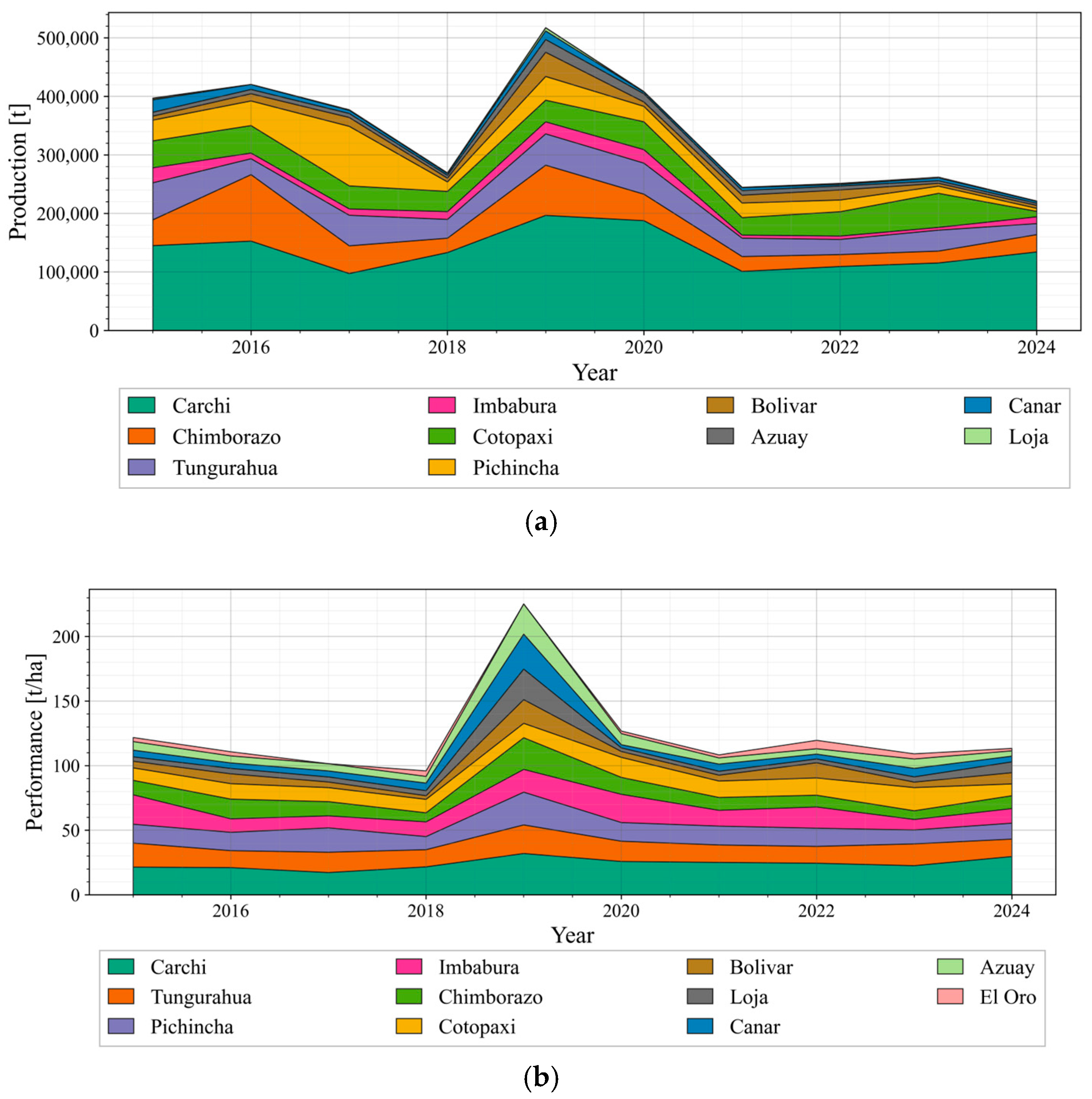
Ecuador is an Andean country where potato cultivation is concentrated along the Sierra; in a context of socioeconomic and institutional challenges, production and yields show marked territorial heterogeneity, influenced by agroecological, technological, and socioeconomic factors [37]. Figure 1 shows the temporal evolution of potato production and yields between 2013 and 2024 [38].

It is observed that Carchi concentrates the highest production values, reaching peaks close to 200 thousand tons (t) in the years 2018 and 2020, with yields above 30 tons per hectare (t/ha), which confirms its historical role as the main producing area of the country, not only for its planted area, but also for its productive efficiency compared to the rest of the provinces. Provinces such as Azuay and Chimborazo show intermediate values, while Bolívar and Cañar show marginal levels in both variables. On the other hand, Cotopaxi, El Oro, Imbabura, Loja, Pichincha and Tungurahua show different dynamics. Cotopaxi and Tungurahua stand out with productions exceeding 100 thousand tons in certain years and yields above 20 t/ha, while Loja and El Oro show a reduced participation and low yields compared to the other provinces.

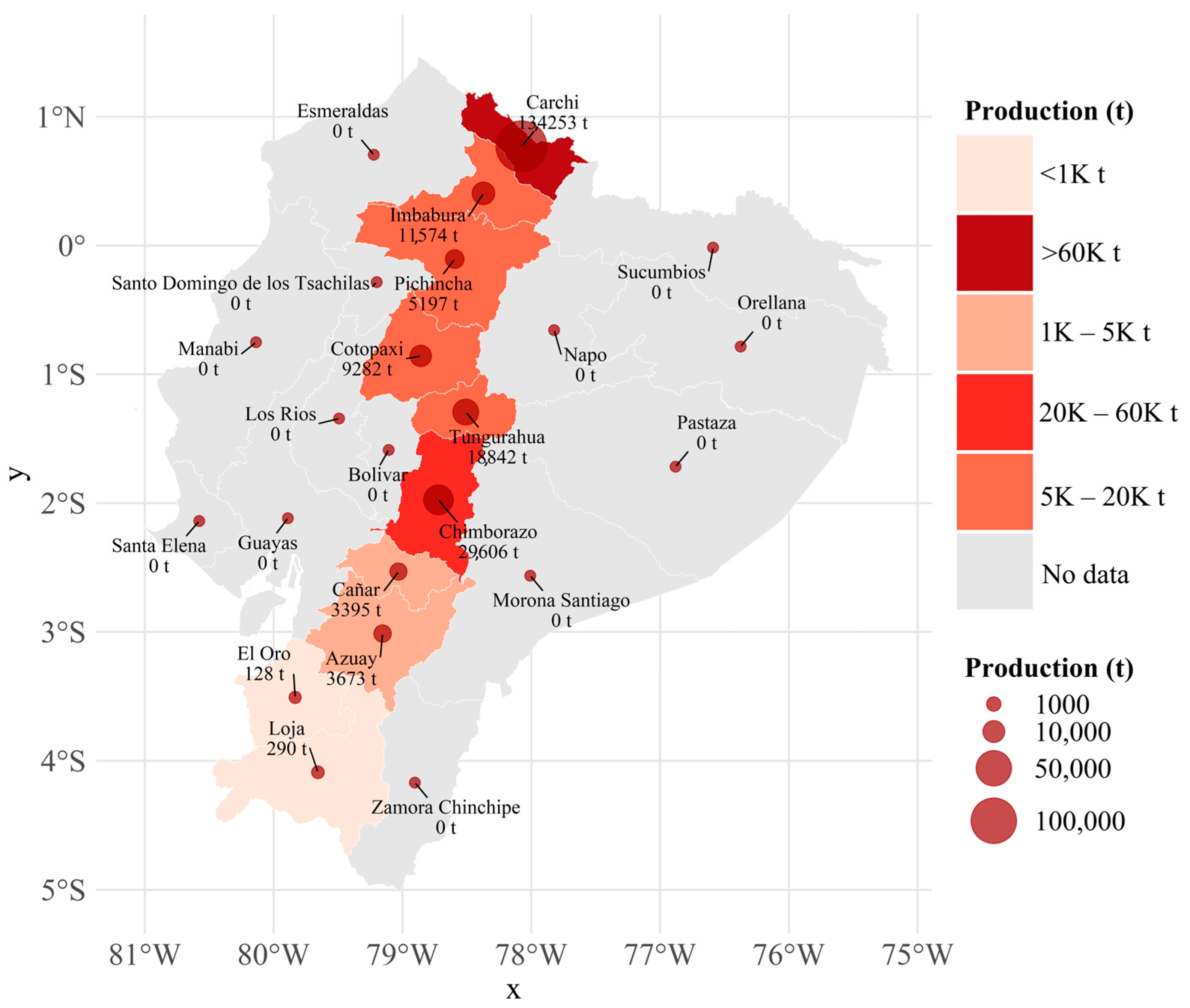
Figure 2 shows the set of geospatial results for the year 2024, showing that Carchi, Cotopaxi and Tungurahua are the most relevant provinces for national potato production, combining high production volumes with relatively high yields. These regional differences are key to understanding the spatial distribution of potato production in the country and to orienting agricultural policy strategies to strengthen food security.

The crops under study are in the central highlands of Ecuador, specifically in the province of Cotopaxi, where several technical agricultural projects are currently being developed. For the analysis, two test plots were established, each with an approximate area of two hectares, which were monitored from field preparation to tuber maturation.

3. Methodology

This study adopts a hybrid quantitative methodology that integrates two complementary analytical frameworks. First, an attributional life cycle assessment (LCA) is conducted to build the life cycle inventory and quantify the environmental impact profiles using the EF 3.0 method across 25 midpoint impact categories. Within this set, climate change is reported as kilograms of carbon dioxide equivalent (kg CO₂-eq) and is interpreted together with the remaining categories as part of a multi-impact assessment. Second, a machine-learning (ML) surrogate model, specifically an artificial neural network (ANN), is trained on the LCA results to enable rapid scenario exploration.

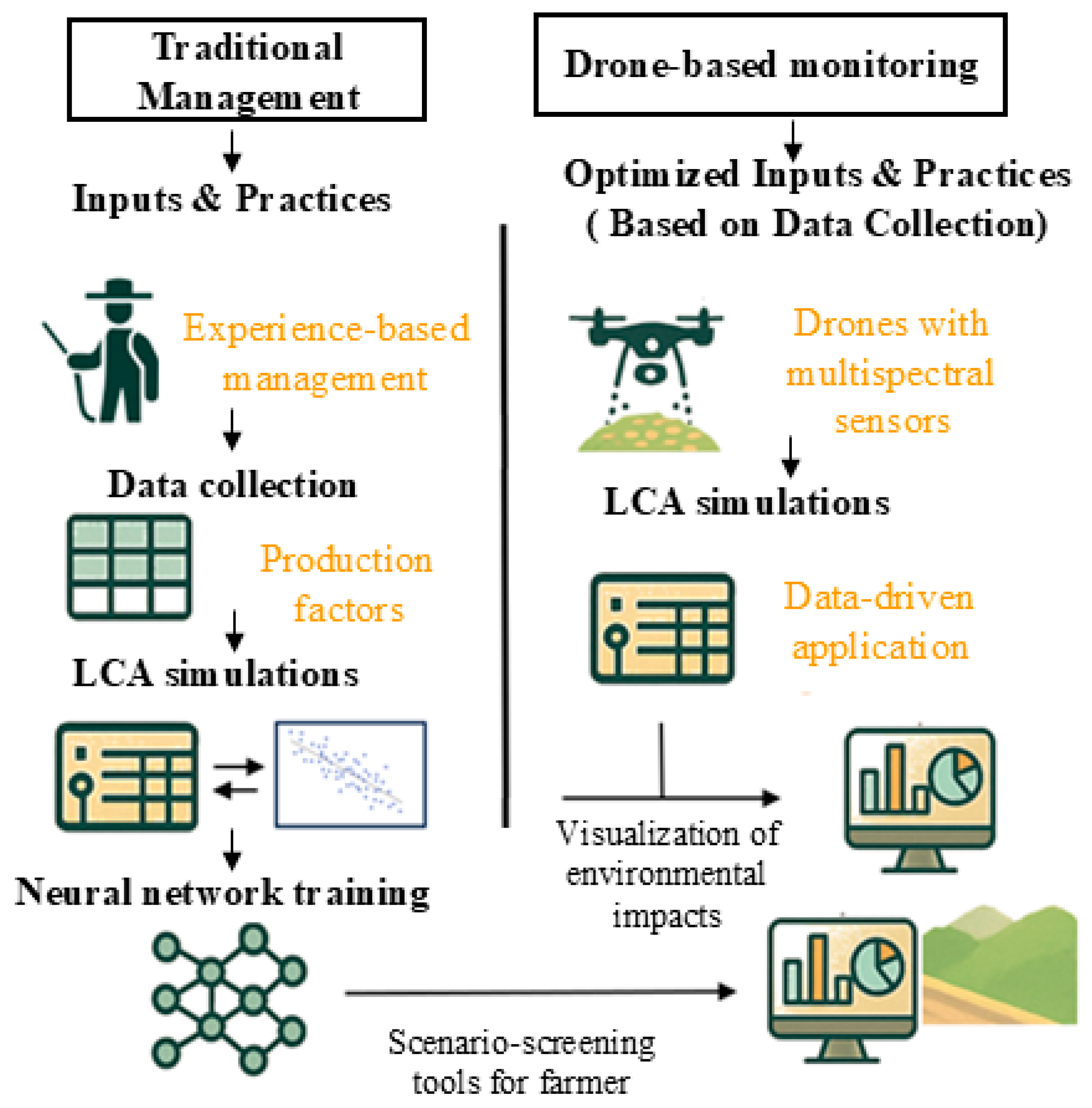
As shown in Figure 3, two scenarios for Andean potato production in Ecuador are compared. The first is a conventional scenario characterized by manual field scouting and broadcast agrochemical application typical of smallholder systems, and the second is a drone-assisted monitoring scenario in which multi-spectral sensing supports targeted input management and reduced agrochemical use. In both cases, the analyzed system covers the crop cycle from planting to tuber maturity, excluding harvesting and transportation stages. Finally, the LCA indicators are used as the training targets for the ANN surrogate, which generalizes the scenario results and enables rapid approximations for new or unobserved conditions (e.g., different provinces), facilitating sensitivity exploration and visualization under the study assumptions.

3.1. UAV-Assisted vs. Conventional Monitoring

A field case study was conducted in Cotopaxi Province (Ecuador) to compare conventional field scouting with UAV-assisted multi-spectral monitoring for potato crop protection decisions. The evaluated variety was the “Chola” potato, one of the most widely cultivated in the area. Two plots of approximately 1.2 hectares (ha) each were considered. Plot A followed conventional management, while Plot B implemented technology-supported management.

In Plot A, four crop-protection interventions were carried out during the productive cycle following the usual local practice based on field scouting and broadcast pesticide applications. In Plot B, the crop was monitored using a DJI Mavic 3M (DJI, Shenzhen, China) UAV equipped with a multi-spectral camera. Five monitoring flights were performed during the productive cycle, and the acquired imagery was processed to generate orthomosaics and crop-condition maps (e.g., vegetation indices) used to identify within-field variability and support targeted pesticide application. For both plots, operational monitoring/intervention time was recorded to enable a standardized comparison of labor requirements and operational performance.

3.2. Functional Unit, Scope and Limits of the System

The functional unit is defined as 1 kg of Andean potato produced. Annual national impacts are obtained by scaling the per-kg results using the corresponding yearly national production, enabling interannual comparisons at the country scale. This scaling approach was intended to provide annual country-level impact estimates for interannual comparison; however, it does not constitute a province-specific yield-normalized aggregation and should, therefore, be interpreted as a national-order estimate. The assessment covers a cradle-to-farm-gate system (from planting to tuber maturity). The system boundary for the LCA includes the following foreground processes: land preparation, planting, fertilizer application (N, P, K), phytosanitary treatment, water use, energy consumption, and drone operation (only for the second scenario). In addition, the inventory includes background (upstream) processes for the production and supply of all inputs (e.g., fertilizers, pesticides, diesel and electricity). Direct field emissions associated with nitrogen fertilization are included by applying the Intergovernmental Panel on Climate Change (IPCC) Tier 1 approach, implemented in OpenLCA as direct nitrous oxide (N₂O) emissions to air from synthetic nitrogen (N) fertilizer [40]. Post-farm transportation, storage, marketing or consumption stages are not considered.

3.3. Model Construction and Key Assumptions in OpenLCA Framework

The LCA of the Andean potato crop in Ecuador was carried out using OpenLCA software (version 2.4), a tool specialized in sustainability assessment of agricultural and industrial processes [41]. Although it is an open-source program, the databases may be free or commercial. In this study, only open-access data were used, specifically the European Life Cycle Database 3.2 (ELCD 3.2 free-no delta version), available for public download [41,42]. All the processes analyzed were modeled ex novo, adapting technical parameters reported in the scientific literature and in specialized reports to the conditions of the Ecuadorian context. For the assessment of environmental impacts, the life cycle impact assessment (LCIA 2.0.2) methods package was used, specifically using the EF 3.0 (adapted) method as the main frame of reference [42,43].

For the scenario simulation of precision agriculture with drones, only the operational phase (flight time and input application) was considered, excluding the equipment manufacturing processes. Agrochemical application rates using drones were standardized according to values reported in previous peer-reviewed studies [44,45].

3.3.1. Potato Crop Input Inventory Using OpenLCA

Two independent life cycle inventories (LCIs) were developed: one for the conventional scenario and one for the scenario with drone-assisted precision agriculture. Both LCIs include (i) upstream processes for the production and supply of inputs (e.g., fertilizers, pesticides, diesel and electricity) and (ii) direct field emissions associated with input use, as modeled in OpenLCA.

Both models incorporated the following elemental flows:

• Nitrogen (N), phosphate (P₂O₅) and potash (K₂O) fertilizer application.
• Water consumption for irrigation.
• Energy demand (electricity).
• Plant material input (potato seed).
• Soil preparation work.
• Diffuse emissions to the soil (by chemical component).

For the scenario with drones, reductions in fertilizer application were calibrated according to scientific evidence reported in the specialized literature, which documents improvements in use efficiency between 15–25%. Based on these studies, conservative reductions of 25% were applied in the application of nitrogen (N), and a conservative 15% reduction for phosphorus (P₂O₅) and potassium (K₂O) relative to conventional doses [44,45].

It is important to note that the field case study was used to document operational aspects of monitoring (e.g., time requirements and workflow performance) and to illustrate drone-assisted scouting under real conditions. However, input-rate reductions in the drone-assisted scenario were not measured directly in the field plots; instead, they were implemented as conservative assumptions based on peer-reviewed evidence reporting improved input-use efficiency under precision agriculture and unmanned UAV-enabled targeting.

Table 1. Foreground life cycle inventory (LCI) of inputs and on-field emissions for potato cultivation in Ecuador (conventional and drone-based VRA scenarios).

No.	Flow	Conventional	Drone (VRA)	References
1	N Fertilizer (urea, as N) [40]	0.015 kg	0.01125 kg (−25%)	[44]
2	P2O5 Fertilizer (DAP)	0.003 kg	0.00255 kg (−15%)	[46,47]
3	K2O Fertilizer (KCl)	0.006 kg	0.00510 kg (−15%)	[48]
4	Machinery diesel	0.005 kg	0.00425 kg (−15%)	[49]
5	Pumping electricity	0.038 kWh	0.0342 kWh (−10%)	[50]
6	Irrigation water	250 kg	225 kg (−10%)	[50,51]
7	Spraying water	10 kg	3.5 kg (−65%)	[45]
8	Pesticide active ingredients (under “Pesticide Application—VRA”)	$\begin{array}{c}\mathrm{Mancozeb} 6.80\times {10}^{-4} \mathrm{kg}\\ \mathrm{Cypermethrin} 6.00\times {10}^{-6} \mathrm{kg}\end{array}$	$\begin{array}{c}\mathrm{Mancozeb} 2.38\times {10}^{-4} \mathrm{kg}\\ \mathrm{Cypermethrin} 2.10\times {10}^{-6} \mathrm{kg}\end{array}$	[44]
9	Occupation, agriculture	0.40 m2·a	0.40 m2·a	[52]
10	Potato seed	0.10 kg	0.10 kg	[53]
11	N2O, direct emission to air (from synthetic N fertilizer; IPCC Tier 1)	$2.36\times {10}^{-4}$ kg	$1.77\times {10}^{-4}$ kg (−25%)	[40]
12	Mancozeb, total on-field emission (all compartments)	$1.90\times {10}^{-4}$ kg	$7.00\times {10}^{-5}$ kg	[54]
13	Cypermethrin, total on-field emission (all compartments)	$5.30\times {10}^{-7}$ kg	$1.85\times {10}^{-7}$ kg	[54]
14	Glyphosate, total on-field emission (all compartments)	$6.00\times {10}^{-5}$ kg	$2.10\times {10}^{-5}$ kg	[55]

Note: LCI: Life Cycle Inventory; VRA: Variable Rate Application; a: annum (year); IPCC: Intergovernmental Panel on Climate Change. Scientific notation: $\propto \times {10}^{-4}.$

presents the inventory of input flows considered for the LCA of the potato crop in Ecuador under two production scenarios, the first conventional method with manual application of agrochemicals and the second with a variable rate application (VRA) method using drones. Agricultural inputs (N, P₂O₅ and K₂O fertilizers, pesticides, water and energy), services per hectare (fertilizer application and phytosanitary treatments) and soil and seed occupancy factors are included. The input reductions in the drone scenario are based on those found in the recent scientific literature and reflect dose reductions due to targeting specific areas of the crop while maintaining the same service operations and soil occupation.

3.3.2. Input Inventory for Drone Use Using OpenLCA

Crop monitoring in the drone scenario was performed using a DJI Mavic 3 Multispectral (Mavic 3M; DJI, Shenzhen, China), a foldable UAV with a net weight of 951 g (including propellers and real-time kinematic module) and a maximum take-off weight of 1050 g. The system offers up to 43 min of maximum flight time (without wind), wind resistance of up to 12 m/s, operation between −10 and 40 °C, and a maximum take-off altitude of 6000 m (without load). The sensor suite integrates a 20 MP RGB camera (CMOS 4/3; field of view 84°; mechanical shutter up to 1/2000 s; max. size 5280 × 3956) and four 5 MP multi-spectral sensors (G 560 ± 16 nm, R 650 ± 16 nm, red edge 730 ± 16 nm, near-infrared 860 ± 26 nm; max. size 2592 × 1944), complemented by an integrated light sensor.

Table 2. Agricultural drone operating system consumables (per 1 h of use).

Process	Input Flow	Quantity	Unit	Source/Assumption
Drone electrical charging	Portugal electricity mix (proxy)	1.10	MJ	[56,58]
Drone maintenance	Copper wire	0.000024	kg	[59]
	Nylon 66 GF 30 compound (PA 66 GF 30)	0.01000	kg	[60]
	PC granulate	0.00030	kg	[60]
	Naphtha	0.0000024	kg	[61]
Drone relocation (1 h use)	Diesel, EU-27 (proxy)	0.60	MJ	Estimated for light transport (5 km round trip for agricultural operations)
Aggregated process	Drone flight hour	1.00	MJ	Output from the electrical charging subprocess
	Drone maintenance service	1.00	MJ (proxy)	Output from the maintenance subprocess
	Drone relocation (1 h use)	1.00	MJ (proxy)	Output from the transport subprocess

presents all the inputs and assumed values used to model the agricultural operation of the drone, structured in three sub-processes: the first called electrical load, the second called preventive and corrective maintenance, and the third named transfer to the area of operation. The electrical consumption per hour of flight was set at 1.10 megajoules per hour (MJ h⁻¹) (≈300 W), in agreement with experimental measurements reported for monitoring multi-drones, e.g., refs. [56,57]. Maintenance was represented by hourly proportional replenishment of specific materials such as, e.g., copper wiring, propellers in 30% glass fiber reinforced polyamide 66 (PA 66 GF30), polycarbonate (PC) housings/encapsulations, and light lubricant (modeled as “lubricating oil” or, alternatively, naphtha as a petrochemical proxy). These values are calculated from the mass of the parts and their replacement intervals. The transfer was modeled as light road transport equivalent to 5 km. All flows were integrated into an aggregated process (“Drone agricultural use hour”) in OpenLCA, using megajoules (MJ) as a proxy for 1 h of service, which allows assessment of the environmental impacts associated with each hour of operation. The Portuguese electricity mix was used as a background proxy for drone charging due to data availability and workflow compatibility in OpenLCA. This choice does not represent Ecuador’s actual electricity matrix, which is more hydro-dominated, and may, therefore, overestimate the climate-related burden of UAV electricity use.

3.3.3. Human Work Evaluation in LCA

Given the scarcity of region-specific data for human labor in agricultural LCA, the environmental burden of manual fieldwork was incorporated using the characterization factors published by [62]. Their study provides impact values for three labor specialization categories. For this analysis, the manual labor (HL-3) category was selected, with an impact factor of 0.41 kg CO₂-eq per work hour, as it accurately reflects the low technification and predominance of manual labor in Ecuadorian potato cultivation. The impacts from skilled (HL-1: 0.52 kg CO₂-eq/h) and technical (HL-2: 0.46 kg CO₂-eq/h) categories were not used, as they were not representative of the studied system. This factor was used as a simplified proxy for comparative scenario modeling. Although it does not capture regional differences in diet, transport, or tool use among Ecuadorian farmers, its contribution is relatively small compared with the dominant environmental burdens associated with agrochemical inputs and related upstream processes in the national-scale results.

3.4. ANN Modeling

A multi-output ANN was developed to approximate agronomic and life-cycle-related outputs of potato production under the two management scenarios evaluated in this study. The surrogate model was designed to provide rapid screening-level estimates of crop performance and environmental indicators derived from OpenLCA, thereby avoiding the need to recalculate the full LCA model for each new scenario combination. Similar machine-learning (ML)-assisted approaches have been reported in the literature to support LCA acceleration, environmental impact prediction, and agro-environmental footprint estimation, including recent review and application studies integrating ML/ANN and LCA [33,34,35,36].

The ANN inputs were intentionally defined as a parsimonious scenario descriptor composed of two variables: (i) cultivated area and (ii) province. Cultivated area was included as a continuous numerical variable because it represents the production scale and directly influences the magnitude of agronomic inputs, labor requirements, and the scaling of environmental burdens. Province was included as a categorical variable because it captures territorial heterogeneity across Ecuador, including broad differences in agroecological context, cropping conditions, and regional production patterns embedded in the annual database. As province is a non-numerical variable, it was transformed using one-hot encoding (OHE).

In the present framework, pesticide use and work-related variables are intermediate scenario-dependent quantities used to construct the LCI and generate the reference LCA results. They are not used as direct input variables for ANN training. Instead, the ANN is trained using cultivated area and province as scenario descriptors to approximate the final agronomic and environmental outputs.

This simplified input design was selected for two reasons. First, these variables were consistently available for the complete annual dataset used in this study (2015–2024). Second, the aim of the ANN was not to reproduce the full agronomic complexity of potato production, but, rather, to act as a computational surrogate for rapid multi-output screening under the assumptions of the study. In that sense, the model should be interpreted as a compact scenario-level predictor that links scale and territorial context with agronomic and environmental outcomes. Nevertheless, the authors acknowledge that these two inputs do not capture all sources of variability. Variables such as climate, soil properties, fertilizer composition, management intensity, and local operational practices could further improve predictive performance, especially for outputs with stronger multi-factorial behavior, such as yield.

The database consisted of structured annual records for the period 2015–2024 [38]. The output variables were grouped into two categories: agronomic indicators and life cycle environmental indicators. In total, the model was trained to predict 29 outputs simultaneously, comprising 4 agronomic indicators and 25 environmental impact indicators derived from the EF method.

Before training, the data were preprocessed to ensure homogeneous scaling among variables. Province was converted to a one-hot encoded vector, while the numerical variable area and all output variables ${\mathrm{y}}^{\left(\mathrm{j}\right)}$ were standardized to zero mean and unit variance. This procedure improved numerical stability during training and avoided dominance of variables with larger scales. The encoding and standardization steps are formalized in Equations (1)–(3), where ${\mathrm{a}}_{\mathrm{i}}$ denotes the one-hot representation of province and ${\mathrm{z}}_{\mathrm{i}}$ denotes the combined input vector.

$${\mathrm{a}}_i=\mathrm{one} \mathrm{hot}\left({\mathrm{Province}}_i\right) \in , {\mathrm{R}}^{\mathrm{K}}.$$

(1)

$${\mathrm{Area}}_i^{\prime }={\displaystyle \frac{{\mathrm{Area}}_i-\mathsf{\mu }\mathrm{Area}}{{\mathsf{\sigma }}_{\mathrm{Area}}}}, {\mathrm{y}}_i^{\prime (j)}={\displaystyle \frac{{\mathrm{y}}_i^{\left(j\right)}-{\mathsf{\mu }}_{y^{\left(j\right)}}}{{\mathsf{\sigma }}_{{\mathrm{y}}^{\left(j\right)}}}} , j=1,\text{…},29 .$$

(2)

$${\mathrm{z}}_i={[\mathrm{Area}}_i^{\prime }{\mathrm{a}}_i] \in {\mathrm{R}}^{1+\mathrm{k}}, \mathrm{k}=11.$$

(3)

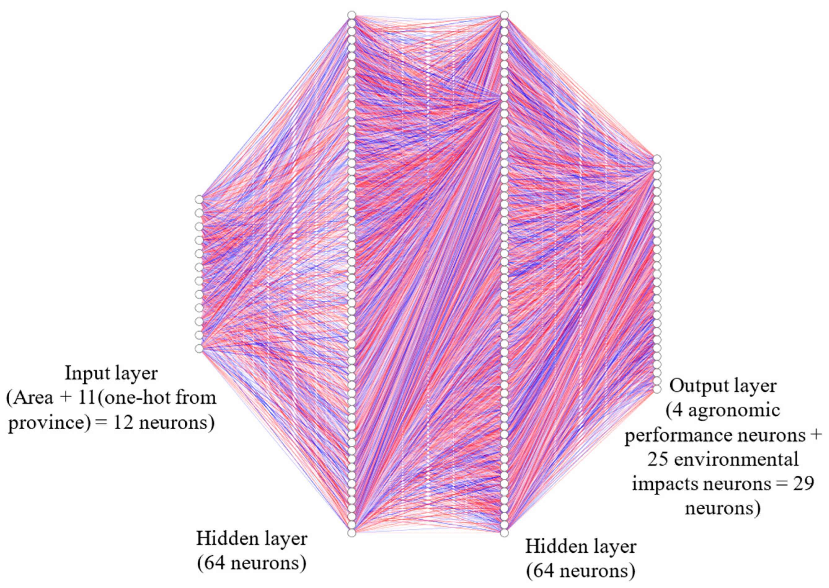
Figure 4 shows the architecture of the ANN. The model is a multi-layer perceptron with an input vector formed by the cultivated area and the one-hot encoding of province ($\mathrm{K}=11$), yielding 12 input neurons. The network contains two hidden layers with 64 rectified linear unit (ReLU) units each, followed by L2 regularization and dropout (0.10) to improve generalization. The output layer contains 29 neurons representing the agronomic and OpenLCA-derived environmental indicators. This architecture was selected because it provides sufficient flexibility to capture non-linear relationships between compact scenario descriptors and multiple output variables while keeping the model computationally efficient.

To reduce overfitting and improve generalization, standard regularization and convergence control strategies were applied during training, such as dropout rate = 0.10 (keep probability = 0.90) [63], L2/weight decay regularization on weights [64], and optimization with Adam [65,66]. Additionally, early stopping was applied by monitoring the validation loss (val_loss) with a patience of 10 epochs and restoring the best weights.

An adaptive learning rate adjustment using ReduceLROnPlateau (Keras callback, TensorFlow 2.15.0) was used, reducing the learning rate when validation loss stopped improving, which helps stabilize training and prevent overfitting [67]. These decisions are in line with classical approximation and neural network fundamentals [68]. To assess temporal robustness, an LOYO scheme was implemented where, in each iteration, one full year was reserved as a test set and the remaining years were used for training; within the training, 10% was separated for internal validation and early stopping criteria. This approach, related to group cross-validation, reduces dependence on a single partition and allows the reporting of performance by year and aggregated summaries using unitless metrics (explained variance score (EVS), weighted/macro-R², and Pearson correlation), complemented by relative error measures (weighted absolute percentage error (WAPE) and symmetric mean absolute percentage error (sMAPE)). Scale-dependent errors (e.g., mean absolute error (MAE)/root mean squared error (RMSE)) are reported per output due to heterogeneous units and ranges across targets, using a reproducible workflow in Python 3.12 with scikit-learn 1.3.2 and TensorFlow 2.15.0/Keras [68,69,70]. Although this grouped temporal validation strategy evaluates out-of-year generalization, it does not imply full independence among years, as interannual autocorrelation in climate conditions and production practices may still be present.

To contextualize the surrogate-model performance, two standard regressors were trained under the same LOYO split: (i) Ridge regression as a linear baseline and (ii) a random forest regressor as a non-linear baseline. Hyperparameters were selected using the training split (10% internal validation), and the same evaluation metrics (EVS, weighted/macro-R², Pearson, WAPE, and sMAPE) were computed to enable a fair comparison. Because the model is trained on LCA-derived outputs, it inherits the assumptions and uncertainties of the underlying inventory and impact assessment; therefore, it is intended as a surrogate for rapid scenario screening rather than a direct predictor of measured environmental burdens.

4. Results

4.1. Analysis of Intervention Time and Productivity

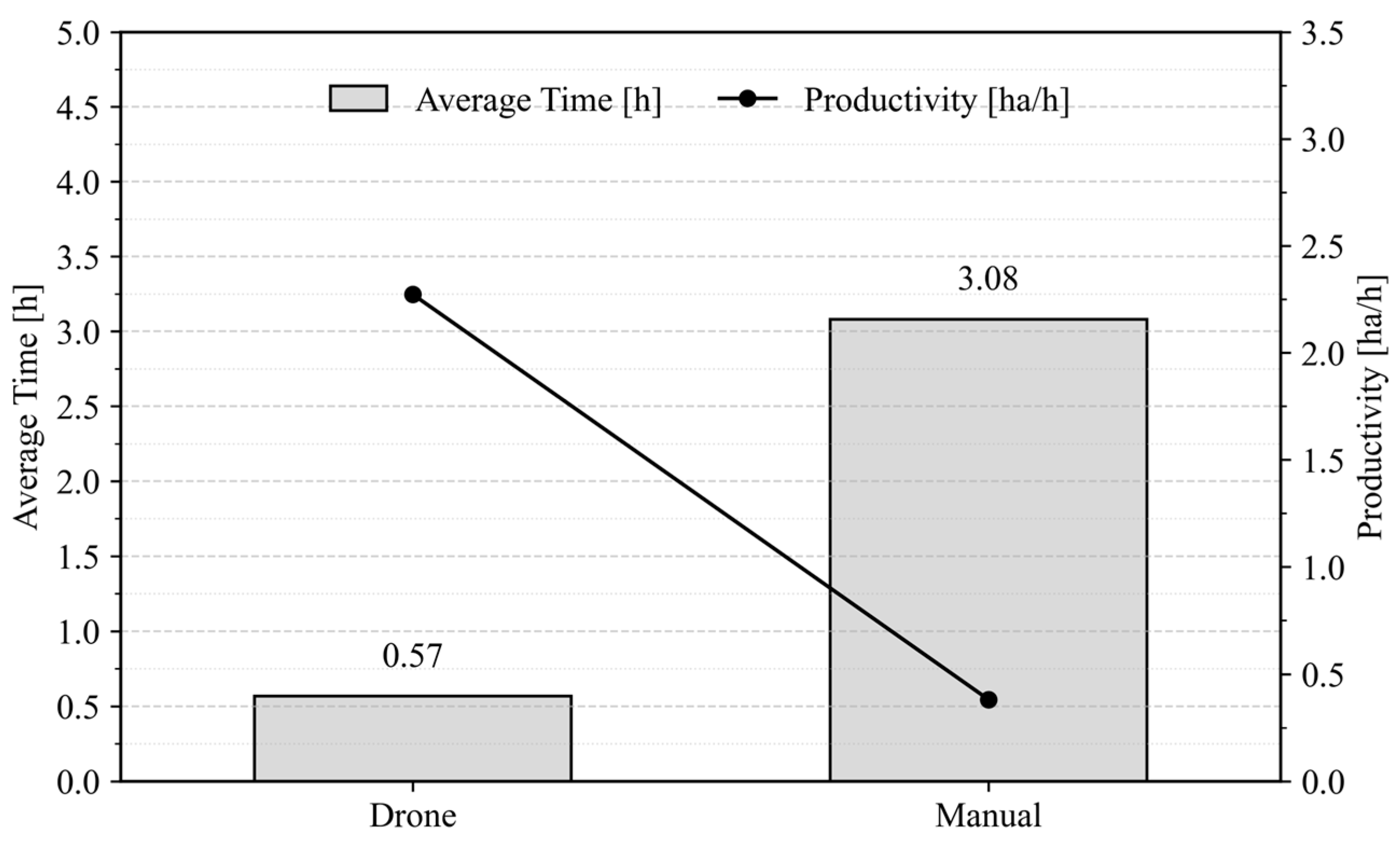
Figure 5 summarizes the operational comparison between unmanned UAV-assisted monitoring and conventional field scouting. For plots of approximately 1.2 hectares (ha), UAV-assisted monitoring reduced the average intervention time from 3.08 h to 0.57 h per day. Accordingly, operational productivity increased from 0.38 hectares per hour (ha/h) under conventional scouting to 2.27 ha/h with UAV-assisted monitoring. This value specifically represents the in-field data acquisition time (setup and flight), excluding computational post-processing, to ensure a comparable operational baseline with manual scouting.

4.2. Environmental Impact Assessment of Potato Production Scenarios

In the present comparison, cultivated area was held constant across scenarios; therefore, land-use impacts do not reflect hypothetical yield-driven reductions in land demand. The results of the national-scale LCA for potato cultivation under the conventional management scenario are presented in

Table 3. Annual evolution of the environmental impact categories of potato planting and fertilization in Ecuador (2015–2024), under a simulation scenario with indiscriminate use of fertilizers, using OpenLCA (bold values indicate the highest value in each impact category).

Impact Category	Reference Unit	2015	2016	2017	2018	2019	2020	2021	2022	2023	2024
Human toxicity, non-cancer—inorg.	CTUh	0.021851	0.023143	0.020752	0.014815	0.028473	0.02247	0.013467	0.013837	0.01442	0.012172
Land use	Pt	$8.49\times {10}^9$	$8.99\times {10}^9$	$8.06\times {10}^9$	$5.75\times {10}^9$	$1.11\times {10}^{10}$	$8.73\times {10}^9$	$5.23\times {10}^9$	$5.37\times {10}^9$	$5.6\times {10}^9$	$4.73\times {10}^9$
Resource use, fossils	MJ	$9.14\times {10}^8$	$9.68\times {10}^8$	$8.68\times {10}^8$	$6.19\times {10}^8$	$1.19\times {10}^9$	$9.4\times {10}^8$	$5.63\times {10}^8$	$5.79\times {10}^8$	$6.03\times {10}^8$	$5.09\times {10}^8$
Climate change—Fossil	kg CO2 eq	76,993,713	81,545,362	73,121,659	52,200,777	$1.0\times {10}^8$	79,176,423	47,453,804	48,755,736	50,811,726	42,890,500
Resource use, minerals and metals	kg Sb eq	0.069313	0.073411	0.065827	0.046994	0.090318	0.071278	0.04272	0.043892	0.045743	0.038612
Eutrophication, marine	kg N eq	53,272.44	56,421.75	50,593.34	36,118.05	69,416.03	54,782.67	32,833.59	33,734.4	35,156.95	29,676.21
Ecotoxicity, freshwater—organics	CTUe	7,812,749	8,274,617	7,419,842	5,296,946	10,180,312	8,034,234	4,815,259	4,947,369	5,155,996	4,352,209
Acidification	mol H+ eq	441,451.5	467,548.9	419,250.7	299,298.6	575,228.3	453,966.3	272,081.4	279,546.1	291,334.4	245,917.2
Ecotoxicity, freshwater—metals	CTUe	50,016,147	52,972,959	47,500,809	33,910,324	65,172,961	51,434,064	30,826,627	31,672,379	33,007,977	27,862,243
Water use	m3 depriv.	$4.77\times {10}^9$	$5.05\times {10}^9$	$4.53\times {10}^9$	$3.24\times {10}^9$	$\mathbf{6.22}\mathbf{\times }{\mathbf{10}}^{\mathbf{9}}$	$4.91\times {10}^9$	$2.94\times {10}^9$	$3.02\times {10}^9$	$3.15\times {10}^9$	$2.66\times {10}^9$
Ionizing radiation	kBq U-235	5,549,231	5,877,286	5,270,157	3,762,309	7,230,861	5,706,547	3,420,177	3,514,012	3,662,195	3,091,282
Human toxicity, non-cancer—metals	CTUh	0.689984	0.730774	0.655285	0.467801	0.899076	0.709545	0.425261	0.436928	0.455353	0.384366
Particulate matter	disease inc.	2.957552	3.132394	2.808815	2.005183	3.853804	3.041396	1.822838	1.872849	1.951826	1.647549
Climate change	kg CO2 eq	76,993,713	81,545,362	73,121,659	52,200,777	$\mathbf{1.0}\mathbf{\times }{\mathbf{10}}^{\mathbf{8}}$	79,176,423	47,453,804	48,755,736	50,811,726	42,890,500
Eutrophication, freshwater	kg P eq	59,741.33	63,273.07	56,736.91	40,503.88	77,845.25	61,434.95	36,820.59	37,830.79	39,426.08	33,279.8
Ozone depletion	kg CFC11 eq	3.506974	3.714296	3.330607	2.377685	4.569722	3.606394	2.161466	2.220767	2.314415	1.953612
Photochemical ozone formation	kg NMVOC	146,990.7	155,680.4	139,598.5	99,657.89	191,534.6	151,157.8	90,595.31	93,080.87	97,006.01	81,883.39
Ecotoxicity, freshwater—inorganics	CTUe	17,489,053	18,522,956	16,609,520	11,857,360	22,788,908	17,984,854	10,779,089	11,074,822	11,541,838	9,742,539
Human toxicity, non-cancer	CTUh	0.712263	0.75437	0.676443	0.482906	0.928106	0.732455	0.438992	0.451036	0.470056	0.396777
Ecotoxicity, freshwater	CTUe	69,067,750	73,150,838	65,594,297	46,827,073	89,997,931	71,025,765	42,568,768	43,736,675	45,581,014	38,475,223
Eutrophication, terrestrial	mol N eq	799,240.7	846,489.6	759,046.5	541,875.2	1,041,441	821,898.6	492,598.8	506,113.7	527,456.1	445,229
Human toxicity, non-cancer—organics	CTUh	0.002353	0.002492	0.002235	0.001596	0.003066	0.00242	0.00145	0.00149	0.001553	0.001311
Human toxicity, cancer—metals	CTUh	0.034435	0.036471	0.032703	0.023347	0.04487	0.035411	0.021224	0.021806	0.022725	0.019183
Human toxicity, cancer—organics	CTUh	0.001524	0.001614	0.001447	0.001033	0.001986	0.001567	0.000939	0.000965	0.001006	0.000849
Human toxicity, cancer	CTUh	0.035959	0.038085	0.034151	0.02438	0.046856	0.036979	0.022163	0.022771	0.023731	0.020032

. Across the 25 environmental impact categories evaluated for the period 2015–2024, a consistent temporal pattern is observed, with impact values reaching a maximum in 2019 and subsequently declining to a minimum in 2024. Relative to 2015, the 2019 peak represents an increase of approximately 30%, while the cumulative reduction between 2019 and 2024 is close to −57%, corresponding to an average annual decrease of about −6% during this period.

The coincidence of the 2019 peak and the sustained decline thereafter, with similar relative magnitudes across all impact categories, indicates that the temporal evolution of the results is primarily driven by changes in the total national potato production volume, rather than by variations in process-specific intensities. Consequently, the observed reduction in environmental indicators should not be interpreted as an improvement in technological or operational efficiency, but, rather, as the effect of reduced production levels. This reduction is consistent with reported decreases in potato production in Ecuador during recent years, potentially linked to adverse climatic conditions, including winter events and the influence of the El Niño phenomenon [8,10].

The national-scale LCA results for the scenario involving drone-based crop monitoring and targeted input application are presented in

Table 4. Annual evolution of the environmental impact categories of potato planting and fertilization in Ecuador (2015–2024), under a simulation scenario with drone use and targeted fertilizer application, using OpenLCA (bold values indicate the highest value in each impact category).

Impact Category	Reference Unit	2015	2016	2017	2018	2019	2020	2021	2022	2023	2024
Human toxicity, non-cancer—inorganics	CTUh	0.01907	0.020197	0.018111	0.012929	0.024849	0.019611	0.011753	0.012076	0.012585	0.010623
Land use	Pt	$8.48\times {10}^9$	$8.98\times {10}^9$	$8.05\times {10}^9$	$5.75\times {10}^9$	$\mathbf{1.1}\mathbf{\times }{\mathbf{10}}^{\mathbf{10}}$	$8.72\times {10}^9$	$5.23\times {10}^9$	$5.37\times {10}^9$	$5.6\times {10}^9$	$4.72\times {10}^9$
Resource use, fossils	MJ	$8.16\times {10}^8$	$8.64\times {10}^8$	$7.75\times {10}^8$	$5.53\times {10}^8$	$\mathbf{1.06}\mathbf{\times }{\mathbf{10}}^{\mathbf{9}}$	$8.39\times {10}^8$	$5.03\times {10}^8$	$5.17\times {10}^8$	$5.38\times {10}^8$	$4.54\times {10}^8$
Climate change—Fossil	kg CO2 eq	67,254,416	71,230,305	63,872,156	45,597,655	87,635,087	69,161,024	41,451,149	42,588,393	44,384,311	37,465,078
Resource use, minerals and metals	kg Sb eq	0.060092	0.063644	0.05707	0.040741	0.078302	0.061795	0.037037	0.038053	0.039657	0.033475
Eutrophication, marine	kg N eq	45,786.69	48,493.47	43,484.05	31,042.8	59,661.81	47,084.7	28,219.87	28,994.1	30,216.76	25,506.16
Ecotoxicity, freshwater—organics	CTUe	1,405,238	7,441,557	6,672,838	4,763,668	9,155,394	7,225,375	4,330,475	4,449,285	4,636,908	3,914,043
Acidification	mol H+ eq	386,819.8	409,687.5	367,366.4	262,259	504,041	397,785.8	238,410	244,950.9	255,280.3	215,483.7
Ecotoxicity, freshwater—metals	CTUe	44,222,832	46,837,159	41,998,842	29,982,528	57,624,049	45,476,513	27,256,013	28,003,802	29,184,700	24,634,990
Water use	m3 depriv.	$4.23\times {10}^9$	$4.48\times {10}^9$	$4.02\times {10}^9$	$2.87\times {10}^9$	$\mathbf{5.52}\mathbf{\times }{\mathbf{10}}^{\mathbf{9}}$	$4.35\times {10}^9$	$2.61\times {10}^9$	$2.68\times {10}^9$	$2.79\times {10}^9$	$2.36\times {10}^9$
Ionizing radiation	kBq U-235 eq	4,876,947	5,165,258	4,631,683	3,306,509	6,354,849	5,015,205	3,005,826	3,088,293	3,218,524	2,716,776
Human toxicity, non-cancer—metals	CTUh	0.62736	0.664448	0.59581	0.425342	0.817475	0.645146	0.386663	0.397272	0.414024	0.34948
Particulate matter	disease inc.	2.614973	2.769563	2.483465	1.772919	3.407411	2.689106	1.611696	1.655914	1.725742	1.45671
Climate change	kg CO2 eq	67,254,416	71,230,305	63,872,156	45,597,655	87,635,087	69,161,024	41,451,149	42,588,393	44,384,311	37,465,078
Eutrophication, freshwater	kg P eq	50,789.03	53,791.53	48,234.83	34,434.33	66,180.06	52,228.86	31,302.98	32,161.8	33,518.04	28,292.79
Ozone depletion	kg CFC11 eq	3.082097	3.264302	2.927097	2.089623	4.016091	3.169472	1.8996	1.951717	2.034019	1.716928
Photochemical ozone formation	kg NMVOC eq	127,090.8	134,604	120,699.3	86,165.97	165,604.2	130,693.7	78,330.31	80,479.37	83,873.12	70,797.83
Ecotoxicity, freshwater—inorganics	CTUe	15,407,957	16,318,832	14,633,083	10,446,403	20,077,160	15,844,760	9,496,440	9,756,982	10,168,426	8,583,233
Human toxicity, non-cancer	CTUh	0.646813	0.685051	0.614284	0.438531	0.842822	0.66515	0.398652	0.40959	0.426862	0.360317
Ecotoxicity, freshwater	CTUe	61,036,027	64,644,302	57,966,493	41,381,664	79,532,287	62,766,349	37,618,548	38,650,641	40,280,507	34,001,032
Eutrophication, terrestrial	mol N eq	673,358.5	713,165.6	639,495	456,528.7	877,412	692,447.7	415,013.4	426,399.6	444,380.6	375,104.4
Human toxicity, non-cancer—organics	CTUh	0.000383	0.002229	0.001998	0.001427	0.002742	0.002164	0.001297	0.001332	0.001389	0.001172
Human toxicity, cancer—metals	CTUh	0.030944	0.032773	0.029387	0.020979	0.040321	0.031821	0.019072	0.019595	0.020421	0.017238
Human toxicity, cancer—organics	CTUh	0.00136	0.00144	0.001291	0.000922	0.001772	0.001398	0.000838	0.000861	0.000897	0.000757
Human toxicity, cancer	CTUh	0.032303	0.034213	0.030679	0.021901	0.042092	0.033219	0.01991	0.020456	0.021318	0.017995

. Similar to the conventional scenario, all impact categories exhibit a maximum in 2019 and a minimum in 2024, with comparable relative variations over time. The cumulative decrease between 2019 and 2024 is, again, close to −57%, while the increase from 2015 to 2019 is on the order of 30%, confirming that the temporal behavior is, likewise, dominated by national production trends.

A direct comparison between Table 3 and Table 4 for the same year shows that the drone-based scenario consistently yields lower environmental impact values across most categories. This systematic reduction is attributable to the lower input requirements associated with the targeted application strategy, including reduced fertilizer and agrochemical use. These results indicate that, although production volume governs the overall temporal trend, the adoption of drone-assisted VRA can lead to measurable reductions in environmental burdens when compared to conventional management practices.

4.3. Environmental Impacts per Hour of Agricultural Drone Operation

Table 5. Key indicators per 1 h of operation (EF 3.0).

Impact Category	Unit	Result
Climate change	kg CO2 eq	0.510
Resource use, fossils	MJ	5.524
Water use	m3 deprivation	0.159
Acidification	mol H+ eq	0.00345
Eutrophication, freshwater	kg P eq	1.89 × 10−6

summarizes the most relevant EF 3.0 impact indicators for one hour of monitoring-drone operation, modeled in OpenLCA. Climate change shows the highest contribution (0.51 kg CO₂ eq·h⁻¹), followed by fossil resource use (5.52 MJ·h⁻¹).

The measured coverage rate during field tests for the monitoring drone was approximately 2.27 ha·h⁻¹. Therefore, the climate-change indicator reported in Table 5 can also be expressed per monitored hectare as 0.51 kg CO₂ eq·h⁻¹/2.27 ha·h⁻¹ = 0.225 kg CO₂ eq·ha⁻¹. This value should be interpreted as a reference estimate based on the modeled operating conditions adopted in this study. No explicit sensitivity analysis was performed for parameters such as effective coverage rate, flight speed, battery performance, or equipment aging. This conversion facilitates an order-of-magnitude comparison with operational studies reported in the literature.

Recent field work on spraying operations indicates that spraying drones can reduce energy consumption and carbon footprint compared with tractor spraying, reporting 14.48 kg CO₂ eq·ha⁻¹ for a spraying drone versus 41.28 kg CO₂ eq·ha⁻¹ for tractor spraying in controlled wheat trials [45] (

Table 6. Comparison of climate-change emissions (kg CO₂ eq·ha⁻¹) between the monitoring drone estimated in this study and spraying operations reported in the literature [45].

Operation	Reference Unit	Climate Impact (kg CO2 eq)
Monitoring drone (this study)	1 hectare monitored	0.225
Spraying drone (field, wheat)	1 hectare treated	14.48
Tractor spraying (field, wheat)	1 hectare treated	41.28

). Although monitoring and spraying are different operations, the comparison is useful to contextualize the magnitude of the monitoring-drone footprint. It should be noted, however, that the monitoring-drone value reported here reflects field operation of the UAV and associated modeled operational burdens, and does not explicitly include electricity consumption from office-based image post-processing and computer-assisted analysis. Therefore, the comparison in Table 6 should be interpreted as an operational-order-of-magnitude comparison rather than a full end-to-end comparison of all downstream digital-processing tasks. In this context, the monitoring drone footprint (0.225 kg CO₂ eq·ha⁻¹) is approximately 64× lower than the reported spraying-drone value and 183× lower than tractor spraying for the climate-change indicator [45].

Drone monitoring shows a substantially lower climate footprint per hectare than spraying systems (either drone or tractor). This difference is expected because monitoring does not require transporting large volumes of liquid or operating high-pressure pumps, which are energy-intensive processes in spraying. Instead, monitoring focuses on acquiring high-resolution imagery to identify spatially targeted intervention zones, enabling localized input management in precision agriculture. As a result, monitoring can support downstream reductions in agrochemical use by improving targeting, contributing to lower overall impacts when integrated into farm decision making.

4.4. Comparison of Life Cycle Analysis Between Manual and Drone Monitoring

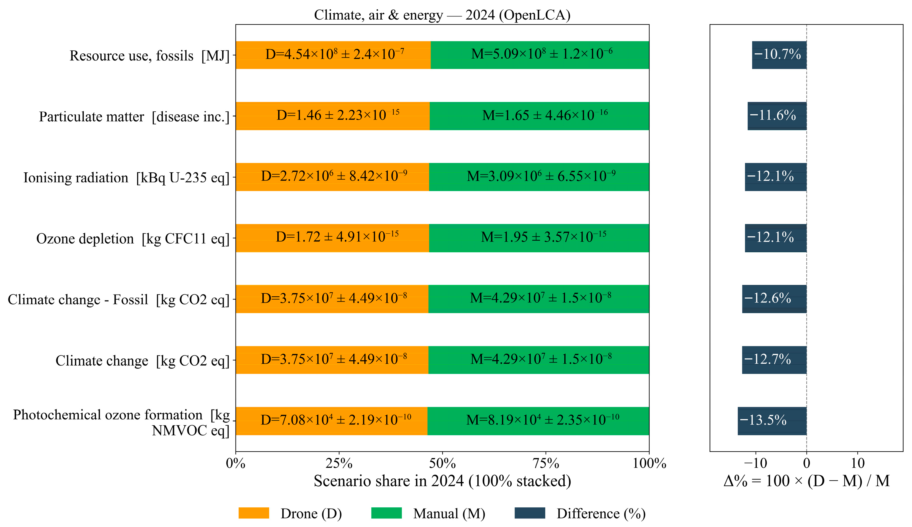
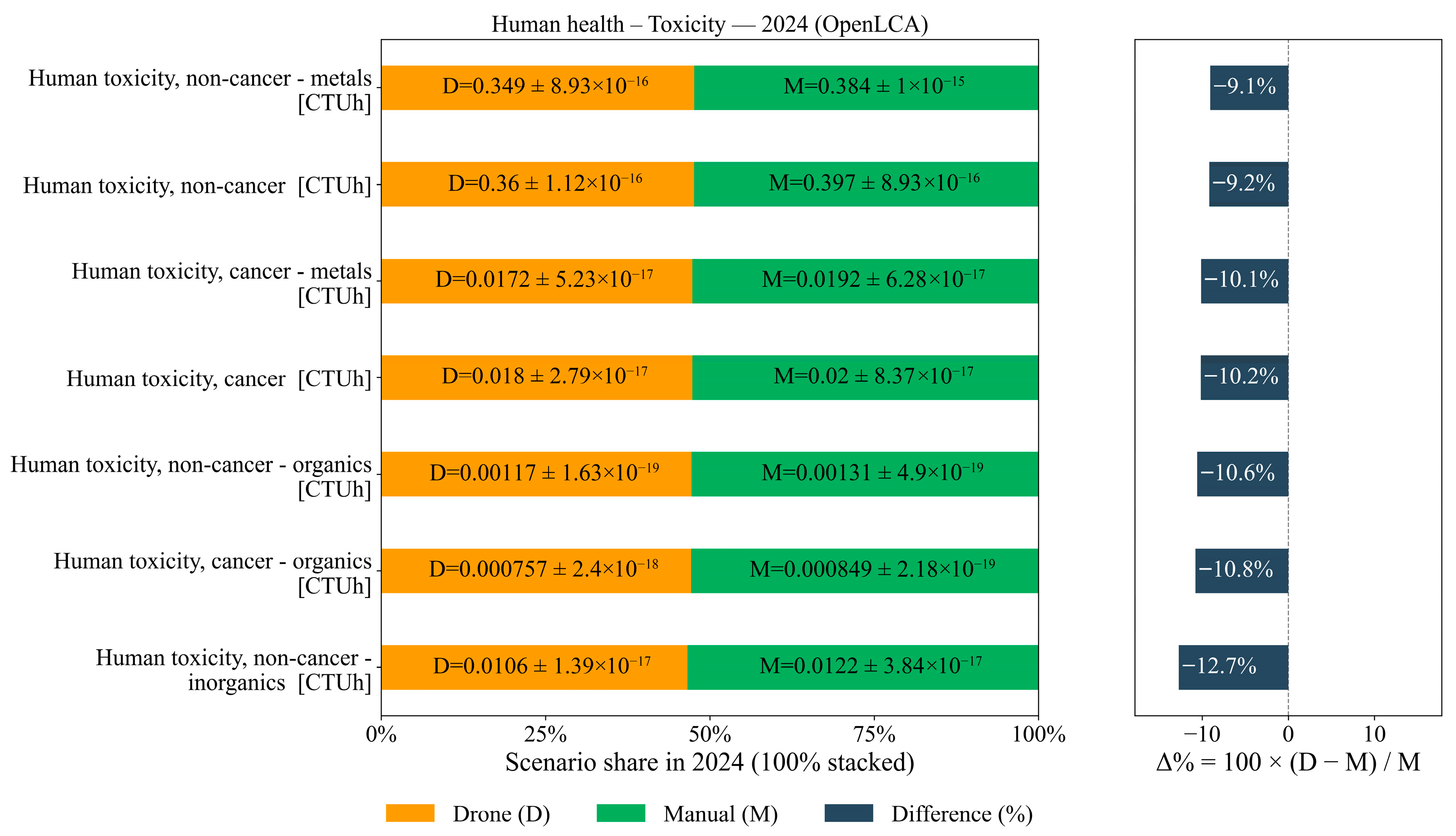
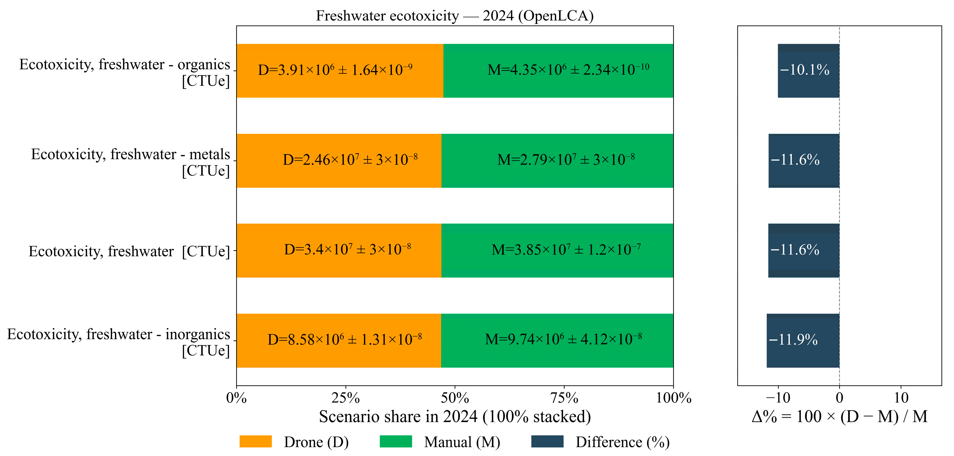
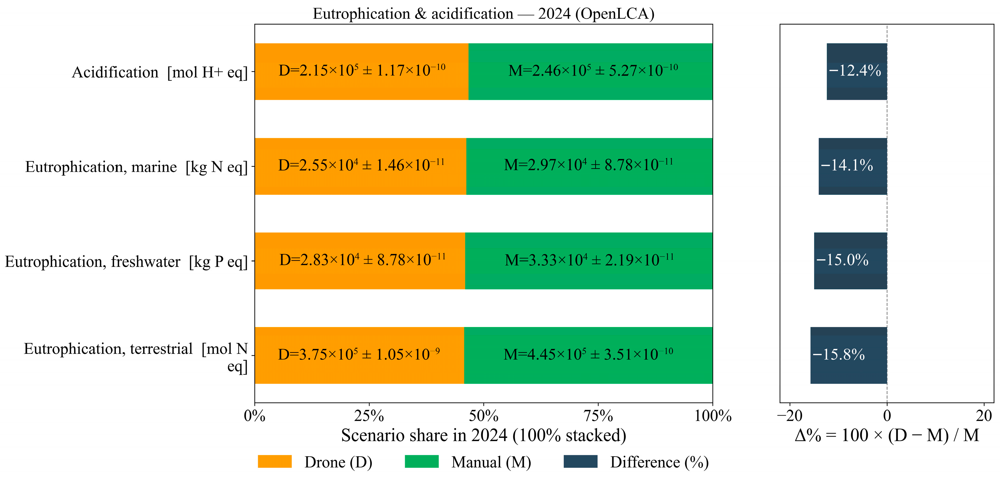
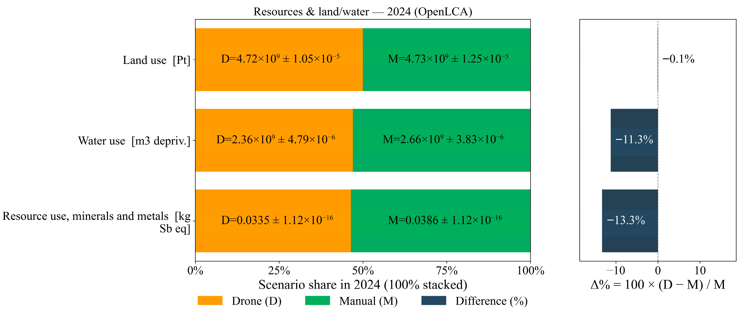
The results of the life cycle analysis for potato production at the national level for the year 2024, carried out using OpenLCA software, are presented below. The impacts obtained were categorized into five families for analysis. The “Climate change” values presented (see Table 3 and Table 4) include contributions from both manual monitoring (14,768.47 kg CO₂ eq) and drone monitoring (3075.244 kg CO₂ eq), calculated from the data obtained in Figure 5. In all figures, the left panel shows the bars stacked at 100% for each category, where the percentages of the drone versus manual scenario are compared, with a statistical uncertainty of ±1 sigma. The right panel includes a third bar of a different color representing the percentage difference between the two.

Figure 6 shows the human health toxicity values, where systematic reductions are observed with drone use in all subcategories. The highest decrease corresponds to “non-cancer–inorganics” (−12.7%), followed by “non-cancer–organics” (−10.6%) and “cancer–organics” (−10.8%). The indicators for “cancer” and “cancer–metals” decreased by −10.2% and −10.1%, respectively, while “non-cancer” and “non-cancer–metals” decreased by −9.2% and −9.1%, respectively. These results demonstrate that targeted application of inputs by drone consistently decreases human toxicity impacts, with a more pronounced effect on inorganic and organic fractions.

Figure 7 shows a reduction in ecotoxicity impacts ranging from −10.1% to −11.9%. Particularly significant were the decreases in the categories of “freshwater–inorganics” (−11.9%), “freshwater–metals” (−11.6%) and “freshwater” (−11.6%). Freshwater–organic compounds also show a significant decrease of −10.1%. This generalized reduction is consistent with the principle of application targeting, which reduces the number of inputs reaching water bodies, showing a clear concordance with the reduction in runoff and leaching phenomena.

Figure 8 shows the largest improvements among the impact categories, with consistent reductions in eutrophication and acidification: terrestrial eutrophication (−15.8%), freshwater eutrophication (−15.0%), marine eutrophication (−14.1%), and acidification (−12.4%). These results suggest that improved dose control and reduced drift with drone application decrease nutrient losses and acidifying emissions across all environmental compartments.

The impacts associated with the climate, air and energy categories are presented in Figure 9. Drone use generates significant reductions in all evaluated categories, including photochemical ozone formation (−13.5%), climate change (−12.7%), climate change–Fossil (−12.6%), stratospheric ozone depletion (−12.1%), ionizing radiation (−12.1%), particulate matter formation (−11.6%) and fossil resource use (−10.7%). These results indicate a systematic decrease in climate- and air-related impacts, consistent with the benefits of a more efficient and focused application of inputs.

Figure 10 presents the results corresponding to the use of natural resources. Significant reductions are observed in the categories of resource use, minerals and metals (−13.3%) and water use (water deprivation, −11.3%). In contrast, land use shows a negligible variation (−0.1%), an expected result given that this impact depends directly on the cultivated area and not on the efficiency of input application. These results show that drone monitoring effectively reduces pressure on abiotic resources such as minerals and water but does not affect the territorial footprint of agricultural activity.

4.5. Surrogate-Model Performance

This section presents the development of an ANN designed to provide a rapid simulation tool for 4 agronomic parameters and 25 environmental impacts, adapted to the realities of Ecuador. The model was trained using data simulated with OpenLCA. The dataset covers the period from 2015 to 2024. Input variables include province and area planted, selected due to the unique agronomic and environmental characteristics of each province. The annual data used for training correspond to all parameters listed in [39]. The environmental impact data feeding the model were simulated in OpenLCA for each province, considering two scenarios: manual monitoring and drone monitoring.

The model was evaluated using LOYO cross-validation. In each of the 10 iterations (2015–2024), nine years were used for training and the remaining year for external testing. Within each training set, an internal subdivision (90% for training, 10% for validation) was applied to control for overfitting using early stopping and adaptive learning rate reduction techniques. This approach allows us to evaluate the temporal generalization capability of the model, so that each year of data remains completely independent of training when used for testing.

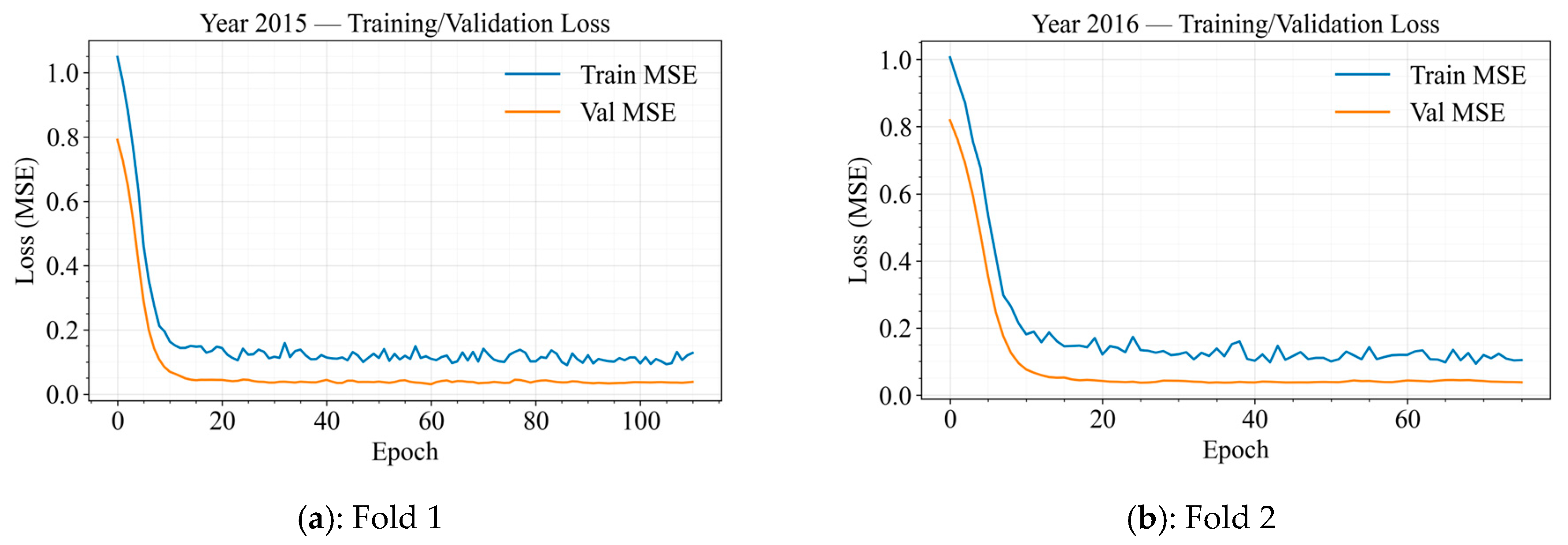
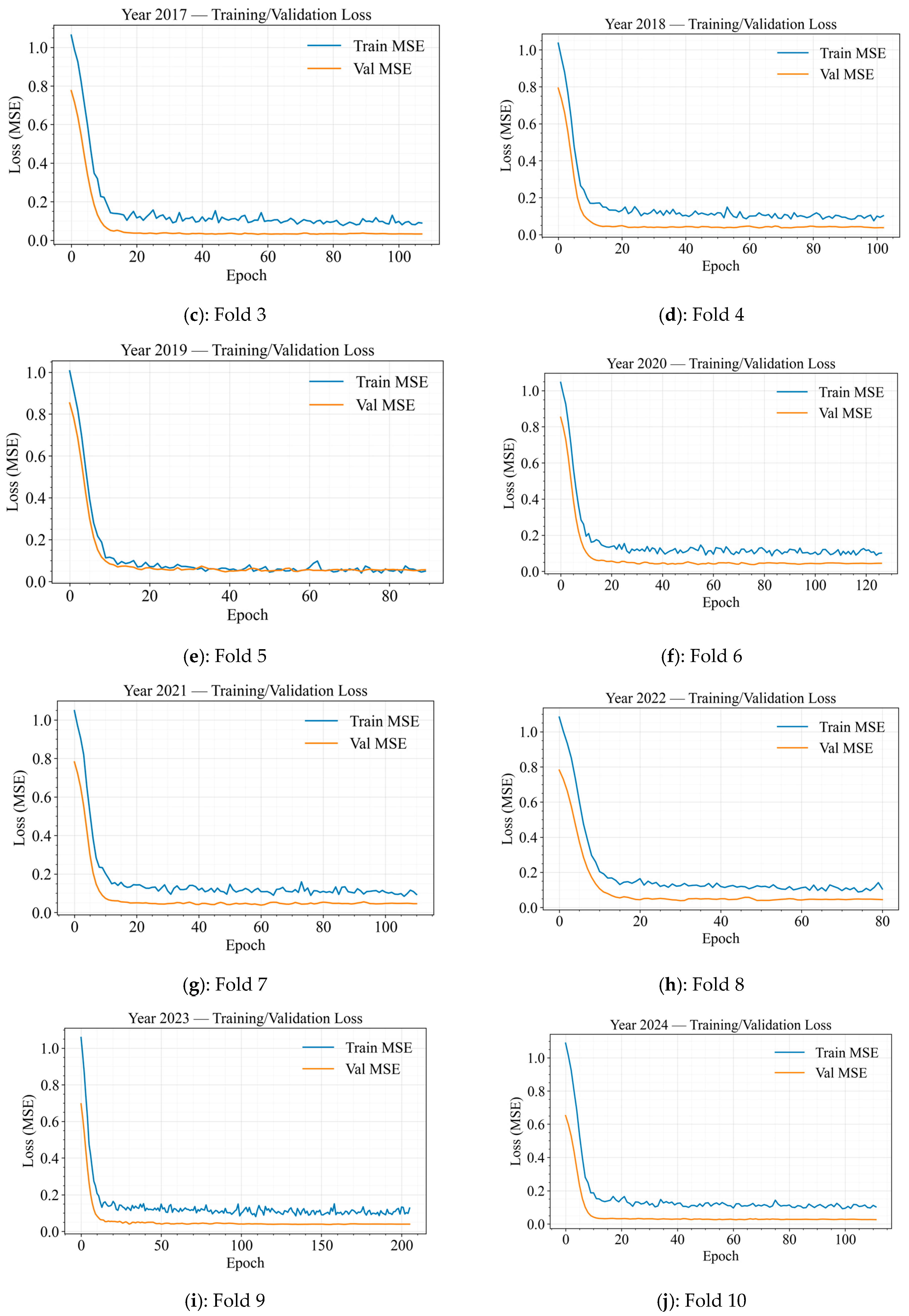
The training behavior of the model is shown in Figure A1, where the loss curves (loss measured as mean squared error, MSE) are plotted as a function of epoch for each fold in the LOYO validation scheme (2015–2024). In each panel, the evolution of both the training loss and the internal validation loss can be observed. In general, the curves show a rapid decrease in error during the first epochs, followed by stabilization, indicating convergence of the model. Among them, Figure A1e, corresponding to the 2019 fold, exhibits the most stable learning behavior. The inclusion of early stopping and adaptive learning-rate reduction helped avoid unnecessary computations and, most importantly, reduced the risk of overfitting, as evidenced by the absence of marked divergences between the training and validation curves.

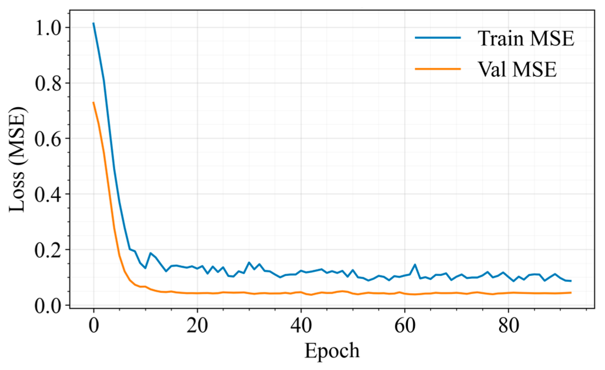
Figure 11 shows the evolution of the loss function MSE during the training of the final model with all data (2015–2024). The initial phase (epochs 0–10) shows a rapid decrease in error, indicating that the model manages to capture relevant patterns in the first iterations. In the intermediate phase (epochs 10–30), the validation loss starts to converge rapidly towards values close to zero, while the training loss stabilizes at a slightly higher level. In the final phase (epochs > 30), both curves remain stable without abrupt increases. The gap between training and validation is small and constant, so it can be said that the ANN has a good generalization.

Table 7. Comparison with baseline models (LOYO average).

Model	EVS	R2_Weighted	R2_Macro	Pearson r	WAPE (%)	sMAPE (%)
Ridge (baseline)	0.871	0.891	0.857	0.972	31.5	66.0
Random Forest (baseline)	0.912	0.984	0.834	0.982	26.8	58.0
ANN surrogate (proposed)	0.933	0.912	0.901	0.987	23.28	51.16

summarizes the surrogate-model performance over the ten evaluated years under the LOYO scheme. The average values of explained variance score (EVS) = 0.934, weighted coefficient of determination (R²) = 0.913, and macro-R² = 0.901 indicate good explanatory power and stable generalization across years. Pearson’s correlation coefficient aggregated across outputs reaches 0.988, suggesting a strong linear association between observed and predicted values.

Because the 29 targets span different physical units and ranges, scale-dependent error metrics (e.g., MAE/RMSE) are not directly comparable when aggregated. Relative metrics support interpretation across heterogeneous outputs, with weighted absolute percentage (WAPE) = 23.28% and symmetric mean absolute percentage error sMAPE = 51.15%. The average MAPE (170%) is inflated by targets with values close to zero; hence, WAPE and sMAPE are prioritized for discussion. Table 7 shows the performance of the proposed model compared to two base models (ridge and random forest) under the LOYO scheme. It can be seen that the ANN surrogate has a better balance between explanatory power and relative error, achieving an EVS = 0.933, weighted R² = 0.912, macro-R² = 0.901, and Pearson’s r = 0.987, along with the lowest percentage errors (WAPE = 23.28% and sMAPE = 51.16%).

The Ridge regression model (linear baseline) shows inferior performance, with EVS = 0.871 and higher relative errors (WAPE = 31.5%, sMAPE = 66.0%), suggesting that a linear relationship does not adequately capture the heterogeneity between provinces and the multi-output dynamics. On the other hand, random forest improves over ridge when compared (WAPE = 26.8%, sMAPE = 58.0%), and maintains high correlation (r = 0.982); however, its macro-R² is lower (0.834), indicating variability in performance between outputs. These results support the use of ANN as a surrogate model for rapid scenario exploration.

Table 8. Overall explanatory power of the neural network; coefficient of determination (R²) per variable considering the entire training and validation series (2015–2024).

Number	Variable	R2
1	Human/drone work [h]	0.987116
2	Human [kg CO2-eq]	0.988794
3	Performance [t/ha]	0.730418
4	Production [t]	0.958230
5	Human toxicity, non-cancer—inorganics [CTUh]	0.957985
6	Land use [Pt]	0.955796
7	Resource use, fossils [MJ]	0.954862
8	Climate change—Fossil [kg CO2 eq]	0.961032
9	Resource use, minerals and metals [kg Sb eq]	0.954529
10	Eutrophication, marine [kg N eq]	0.950143
11	Ecotoxicity, freshwater—organics [CTUe]	0.954608
12	Acidification [mol H+ eq]	0.948355
13	Ecotoxicity, freshwater—metals [CTUe]	0.950882
14	Water use [m3 depriv.]	0.955964
15	Ionising radiation [kBq U-235 eq]	0.957829
16	Human toxicity, non-cancer—metals [CTUh]	0.956687
17	Particulate matter [disease inc.]	0.947910
18	Climate change [kg CO2 eq]	0.958270
19	Eutrophication, freshwater [kg P eq]	0.914608
20	Ozone depletion [kg CFC11 eq]	0.964908
21	Photochemical ozone formation [kg NMVOC eq]	0.957024
22	Ecotoxicity, freshwater—inorganics [CTUe]	0.961423
23	Human toxicity, non-cancer [CTUh]	0.957742
24	Ecotoxicity, freshwater [CTUe]	0.953419
25	Eutrophication, terrestrial [mol N eq]	0.961943
26	Human toxicity, non-cancer—organics [CTUh]	0.951766
27	Human toxicity, cancer—metals [CTUh]	0.955290
28	Human toxicity, cancer—organics [CTUh]	0.954303
29	Human toxicity, cancer [CTUh]	0.961722

presents the coefficient of determination (R²) for each of the 29 target variables over the entire time series. The model exhibits outstanding performance, with 25 of 29 variables (≈86%) showing R² ≥ 0.95. Within this range are included indicators such as Human work (h) (0.987), Human kg CO₂-eq (0.989), Climate change—Fossil (0.961) and Ozone depletion (0.965). A second group of variables reaches R² values in the range 0.91–0.95, such as Eutrophication, freshwater with 0.915. These categories, although they present greater dispersion, maintain an acceptable fit within environmental contexts.

The most difficult variable to estimate is Performance (t/ha), with R² = 0.73. This can be attributed to its multi-factorial nature, involving agronomic, climatic and management factors that are not explicitly represented in the model inputs, as well as to the fact that some provinces record zero production values that, in practice, are not recorded for that period, for example, the province of El Oro (see Figure 1).

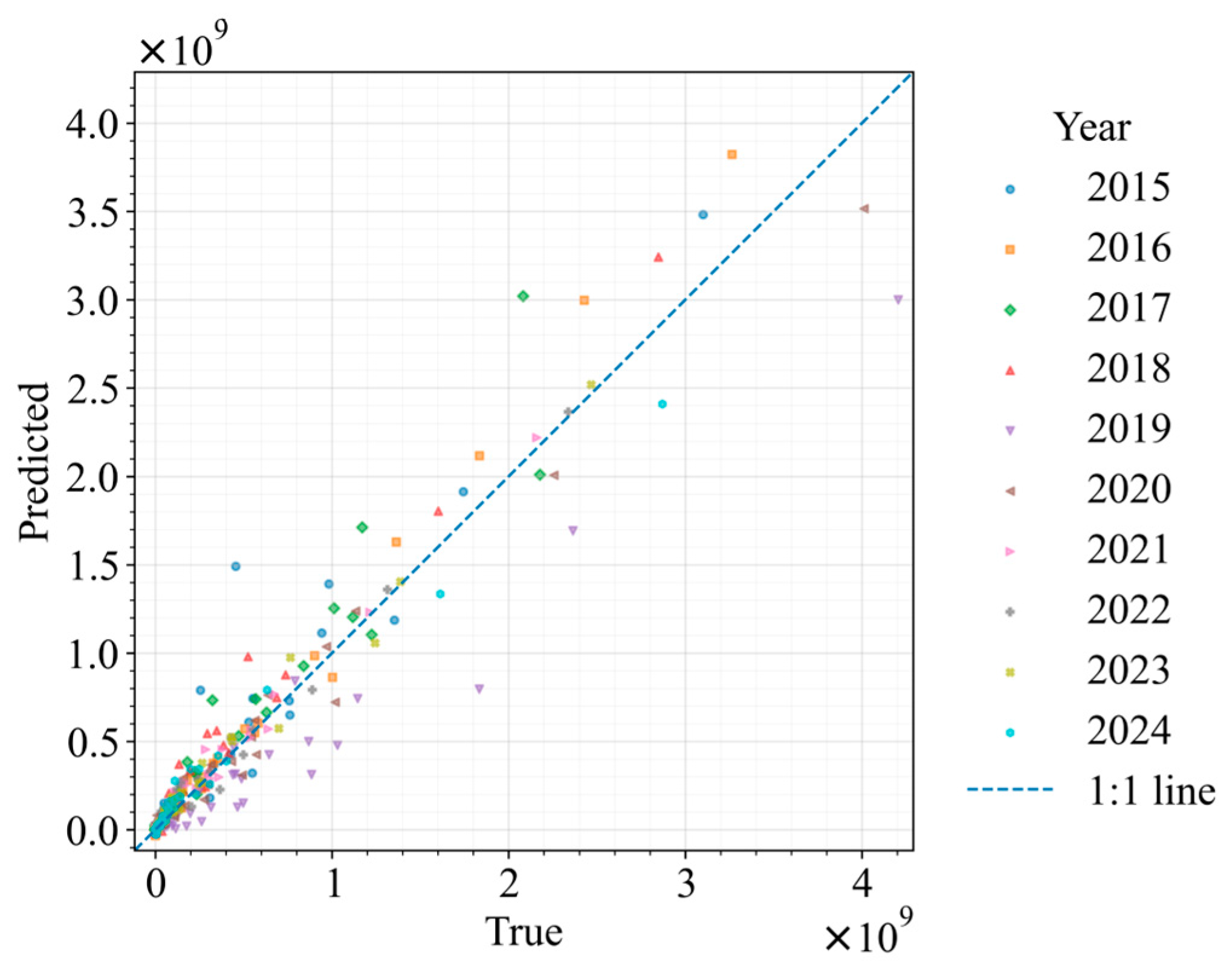
Figure 12 shows the consolidated parity plot of all LOYO folds. Each point corresponds to a (true/estimate) pair of the 29 departures, and the markers encode the test year. The cloud of results aligns closely to the 1:1 line, which indicates an acceptable model and agrees with aggregate metrics such as mean weighted R² ≈ 0.913; EVS ≈ 0.934; Pearson ≈ 0.988. Slight heteroscedasticity is appreciated; the dispersion grows with magnitude, where some points appear above and below the diagonal; this shows residual variability at higher values and/or more complex targets (e.g., yield t/ha). Even so, no marked systematic bias (consistent over- or under-estimation) is observed, and most points remain close to the diagonal.

These results synthesize multi-output performance across the entire series where estimates are close to 1:1 across most of the range, with localized deviations justifying recommendations to include agronomic/climatic covariates for the more difficult targets or log/scale transformations by variable to reduce dispersion at the upper end.

5. Discussion

The results of this study indicate that UAV-assisted monitoring, combined with targeted field interventions, can improve the environmental performance of potato production in Ecuador compared to conventional manual management. In most of the impact categories evaluated, the UAV scenario showed lower impacts on climate change, fossil fuel use, acidification, particulate matter formation, eutrophication, and several categories related to ecotoxicity. This suggests that the environmental benefit of drone-assisted mechanization stems not only from UAV operation but also from the reduction in unnecessary agrochemical applications and a more selective allocation of field interventions. In contrast, land use remained virtually unchanged across scenarios, which is to be expected as land use depends primarily on the cultivated area and not on the monitoring strategy.

From an LCA perspective, these results support the idea that precision agriculture technologies contribute to environmental mitigation not only through direct reductions in input use, but also through lower indirect loads associated with over-application, runoff, and inefficient management. This interpretation is consistent with previous studies that have reported environmental benefits of drone-assisted agricultural operations and machine-learning-supported environmental screening approaches [33,34,35,36,45]. However, the available literature remains more extensive for spraying operations than for monitoring-based strategies, making this contribution relevant for expanding the evidence base in this area

The ANN results also show that the proposed surrogate framework is useful as a rapid multi-output screening tool. The model achieved good agreement with the results derived from the LCA, indicating that compact descriptors at the scenario level can capture a substantial portion of the variability in the modeled agronomic and environmental indicators. The use of cultivated area and province as input variables was intentionally parsimonious, such that the area captures the scale of production, while the province captures the territorial heterogeneity incorporated in the annual database. In this sense, the ANN was not conceived as a full-process agronomic model, but, rather, as a computational surrogate capable of approximating the outputs of the LCA-based flow under the study’s assumptions.

Furthermore, predictive performance was not equally strong for all variables. Outputs related to yield showed comparatively lower accuracy, suggesting that some agronomic responses depend on additional explanatory factors not explicitly represented in the current model, such as climate, soil properties, fertilizer composition, local management intensity, and operational variability. Therefore, although the ANN is suitable for rapid scenario exploration and environmental screening, its outputs should be interpreted within the scope and assumptions of the reference dataset used for training.

Several limitations of the study should be acknowledged. First, the environmental assessment was presented primarily at the national level; further standardization per hectare or per ton would enhance interpretability and comparability with other studies. Second, as the ANN was trained using outputs derived from the LCA, it inherits the assumptions and uncertainties of the inventory and the impact assessment model. Third, a limitation of the present assessment of drone monitoring is that electricity use in the office associated with image post-processing, orthomosaic generation, and computer-assisted analysis was not explicitly inventoried. Future studies should incorporate these subsequent digital-processing loads to provide a more comprehensive comparison between UAV-based monitoring and other agricultural operations. In addition, richer input structures for the ANN should be explored, including climate, soil, and management covariates, as well as sensitivity and uncertainty analyses, with the aim of improving the robustness of both the environmental assessment and the surrogate-model predictions. Finally, future work should extend the present framework toward techno-economic and policy-oriented assessment, particularly to evaluate affordability, adoption barriers, and implementation pathways for smallholder farmers in Ecuador and similar resource-constrained agricultural contexts.

6. Conclusions

This study demonstrates that, for domestic potato production in Ecuador, the adoption of UAV-based monitoring with targeted fertilization constitutes a technically and environmentally preferable alternative to traditional manual management. By 2024, the UAV-informed scenario achieved systematic reductions across most environmental impact families, with median decreases of approximately −14.1% for eutrophication and acidification, −12.1% for climate/air/energy, −11.6% for freshwater ecotoxicity, −10.2% for human health toxicity, and −12.3% for resources/water. The only category with no relevant change was land use (≈−0.1%), which is consistent with the dependence of land occupation on cultivated area rather than on the monitoring approach.

The study also provides an operational reference footprint for UAV-based monitoring of 0.225 kg CO₂ eq·ha⁻¹, derived from 0.51 kg CO₂ eq·h⁻¹ at a coverage rate of 2.27 ha·h⁻¹. This value is substantially lower than values reported in the literature for pesticide spraying operations, namely, approximately 14.48 kg CO₂ eq·ha⁻¹ for drone spraying and 41.28 kg CO₂ eq·ha⁻¹ for conventional tractor spraying. These results highlight the low direct operational burden of monitoring drones and support their use for scenario screening in precision agriculture.

Regarding the multi-output artificial neural network (ANN), trained with OpenLCA-derived agronomic and environmental data from 2015 to 2024, the model successfully emulated 29 environmental and productive outputs with high fidelity. UnderLOYO validation, it achieved explained variance socre (EVS) = 0.934, weighted R² = 0.913, macro-R² = 0.901, Pearson correlation ≈ 0.988, and average weighted absolute percentage (WAPE) ≈ 23%. Approximately 86% of the variables showed R² ≥ 0.95, while the main exception was performance (t/ha) (R² ≈ 0.73), indicating that yield remains more dependent on additional agronomic and climatic covariates. Overall, the proposed approach provides a practical tool for rapid multi-impact scenario assessment and for prioritizing environmentally favorable interventions in Ecuadorian potato systems.

References

1. Bununu, Y.A.; Bello, A.; Ahmed, A. Land cover, land use, climate change and food security. Sustain. Earth Rev. 2023, 6, 16. [Google Scholar] [CrossRef]
2. Smyth, S.J.; Webb, S.R.; Phillips, P.W.B. The role of public-private partnerships in improving global food security. Glob. Food Secur. 2021, 31, 100588. [Google Scholar] [CrossRef]
3. Ahmadu, T.; Abdullahi, A.; Ahmad, K. The role of crop protection in sustainable potato (Solanum tuberosum L.) production to alleviate global starvation problem: An overview. In Animal Husbandry and Nutrition; Yücel, B., Taşkin, T., Eds.; IntechOpen: London, UK, 2021. [Google Scholar] [CrossRef]
4. FAO. The State of Food Security and Nutrition in the World 2018: Building Climate Resilience for Food Security and Nutrition; Food and Agriculture Organization of the United Nations: Rome, Italy, 2018. [Google Scholar]
5. Global Hunger Index. Available online: https://www.globalhungerindex.org/ (accessed on 15 January 2026).
6. Devaux, A.; Goffart, J.-P.; Petsakos, A.; Kromann, P.; Gatto, M.; Okello, J.; Suarez, V.; Hareau, G. Global food security, contributions from sustainable potato agri-food systems. In The Potato Crop; Campos, H., Ortiz, O., Eds.; Springer: Cham, Switzerland, 2020; pp. 3–35. [Google Scholar] [CrossRef]
7. Pumisacho, M.; Sherwood, S. El Cultivo de la Papa en Ecuador; INIAP y CIP: Quito, Ecuador, 2002. [Google Scholar]
8. Serrano-Vincenti, S.; Guamán-Pozo, J.; Chuqui, J.; Tufiño, R.; Franco-Crespo, C. Measuring the effects of climate change on traditional crops in tropical highlands, Ecuador. Front. Sustain. Food Syst. 2025, 9, 1447593. [Google Scholar] [CrossRef]
9. Our World in Data. Potato Production. Available online: https://ourworldindata.org/grapher/potato-production?time=latest (accessed on 14 October 2025).
10. Racines Jaramillo, M.R.; Amagua Bautista, J.M.; Suango Sánchez, V.D.R.; Cuesta Subía, H.X. Producción y Consumo de Papa en Ecuador; INIAP-EESC: Quito, Ecuador, 2023; Available online: https://repositorio.iniap.gob.ec/items/86afb23f-65ad-4e57-bf9c-e694bdaa73fa (accessed on 15 January 2026).
11. PotatoPro. Ecuador: Precios Aumentan por Presión Fitosanitaria. Available online: https://www.potatopro.com/es/news/2024/ecuador-precios-aumentan-por-presi%C3%B3n-fitosanitarias (accessed on 9 July 2024).
12. Hafeez, A.; Husain, M.A.; Singh, S.P.; Chauhan, A.; Khan, M.T.; Kumar, N.; Soni, S.K. Implementation of drone technology for farm monitoring & pesticide spraying: A review. Inf. Process. Agric. 2023, 10, 192–203. [Google Scholar] [CrossRef]
13. Oliveira, R.C.; e Silva, R.D. Artificial intelligence in agriculture: Benefits, challenges, and trends. Appl. Sci. 2023, 13, 7405. [Google Scholar] [CrossRef]
14. Software House. Which Country Has the Best Agricultural Technology in the World? Available online: https://softwarehouse.au/blog/which-country-has-the-best-agricultural-technology-in-the-world/ (accessed on 30 January 2025).
15. Pitla, S.; Bajwa, S.; Bhusal, S.; Brumm, T.; Brown-Brandl, T.M.; Buckmaster, D.R.; Condotta, I.; Fulton, J.; Janzen, T.J.; Karkee, M.; et al. Ground and aerial robots for agricultural production: Opportunities and challenges. Biol. Syst. Eng. 2020, CAST Issue Paper 70. Available online: https://digitalcommons.unl.edu/biosysengfacpub/727/?utm_source=digitalcommons.unl.edu%2Fbiosysengfacpub%2F727&utm_medium=PDF&utm_campaign=PDFCoverPages (accessed on 13 December 2025).
16. Cheng, C.; Fu, J.; Su, H.; Ren, L. Recent advancements in agriculture robots: Benefits and challenges. Machines 2023, 11, 48. [Google Scholar] [CrossRef]
17. Fortune Business Insights. Agriculture Drone Market Size, Share & Industry Analysis, by Offering (Hardware and Software & Services), by Components (Frames, Control Systems, Propulsion System, Navigation System, Camera Systems, and Others), by Payload Capacity (Lightweight Drones (Upto 10 kg), Medium Weight Drones (Upto 10–25 kg), and Heavy Weight Drones (Above 25 kg)), by Application (Monitoring and Mapping, Precision Farming, Irrigation Management, Crop Health Assessment, Planting and Sowing, and Data Collection and Analysis), and Regional Forecast, 2024–2032. Available online: https://www.fortunebusinessinsights.com/agriculture-drones-market-102589 (accessed on 15 January 2026).
18. Virtue Market Research. Latin America Agriculture Drones Market Research Report—Segmentation by Type (Fixed Wing, Rotary Wing), by Component (Hardware, Software, Services), by Application (Crop Management, Field Management, Crop Spraying, Livestock Monitoring, Variable Rate Application (VRA), Others); and Region—Size, Share, Growth Analysis|Forecast (2023–2030). Available online: https://virtuemarketresearch.com/report/latin-america-agriculture-drones-market (accessed on 15 January 2026).
19. Beltrán Barreto, G.X. Antecedentes, Uso y Aplicación de Drones en Colombia como Herramienta Estratégica de Análisis en la Agricultura de Precisión. Bachelor’s Thesis, Universidad de Ciencias Ambientales y Aplicadas (U.D.C.A), Bogotá, Colombia, 2023. Available online: https://repository.udca.edu.co/server/api/core/bitstreams/41675eea-0b1d-4215-801c-9500e5b6f404/content (accessed on 15 January 2026).
20. Rivera, L.B.; Montoya Bonilla, B.; Vidal, F.O. Procesamiento de imágenes multiespectrales captadas con drones para evaluar el índice de vegetación de diferencia normalizada en plantaciones de café variedad Castillo. Cienc. Tecnol. Agropecu. 2021, 20, 1578. [Google Scholar]
21. Cortez Núñez, J.A.; Zepeda Mondragón, F.; García Reyna, M.E.; Hernández León, B.; Aguirre Mendizabal, A. Monitoreo de áreas de cultivo de maíz en la zona noroeste del Estado de México a través de sensores remotos. Rev. Cart. 2024, 109, 7–27. [Google Scholar] [CrossRef]
22. Nazarov, D.; Nazarov, A.; Kulikova, E. Drones in agriculture: Analysis of different countries. BIO Web Conf. 2023, 67, 02029. [Google Scholar] [CrossRef]
23. Agromarketing Latam. Drones en la Agricultura de Latinoamérica. Available online: https://agromarketinglatam.com/drones-en-la-agricultura-de-latinoamerica/ (accessed on 15 January 2026).
24. Suvittawat, A. Investigating farmers’ perceptions of drone technology in Thailand: Exploring expectations, product quality, perceived value, and adoption in agriculture. Agriculture 2024, 14, 2183. [Google Scholar] [CrossRef]
25. Fan, J.; Liu, C.; Xie, J.; Han, L.; Zhang, C.; Guo, D.; McConkey, B.G. Life cycle assessment on agricultural production: A mini review on methodology, application, and challenges. Int. J. Environ. Res. Public Health 2022, 19, 9817. [Google Scholar] [CrossRef] [PubMed]
26. Kowalczyk, Z. Life cycle assessment (LCA) of potato production. E3S Web Conf. 2019, 132, 02003. [Google Scholar] [CrossRef]
27. Mattsson, B.; Wallén, E. Environmental life cycle assessment (LCA) of organic potatoes. Acta Hortic. 2003, 619, 427–435. [Google Scholar] [CrossRef]
28. Timpanaro, G.; Branca, F.; Cammarata, M.; Falcone, G.; Scuderi, A. Life cycle assessment to highlight the environmental burdens of early potato production. Agronomy 2021, 11, 879. [Google Scholar] [CrossRef]
29. Medel Jiménez, F.; Krexner, T.; Gronauer, A.; Kral, I. Life cycle assessment of four different precision agriculture technologies and comparison with a conventional scheme. J. Clean. Prod. 2024, 434, 140198. [Google Scholar] [CrossRef]
30. Milindi, P.S.; Nsenuka, E.E.; Chopra, S.S. Driving sustainability in the sugarcane industry: Life cycle assessment of conventional and emerging spraying technologies in Tanzania. Sci. Total Environ. 2024, 955, 176963. [Google Scholar] [CrossRef]
31. Ramteke, S.V.; Varadwaj, P.K.; Tiwari, V. Optimizing UAV spraying for sustainable agriculture: A life cycle and efficiency analysis in India. Sustainability 2025, 17, 6211. [Google Scholar] [CrossRef]
32. Fariz, T.N.; Basha, S.S. Enhanced crop yield prediction using a hybrid artificial neural network with coati optimization algorithm. Results Eng. 2025, 28, 107529. [Google Scholar] [CrossRef]
33. Salla, J.V.; de Almeida, T.A.; Silva, D.A.L. Integrating machine learning with life cycle assessment: A comprehensive review and guide for predicting environmental impacts. Int. J. Life Cycle Assess. 2025, 30, 2423–2445. [Google Scholar] [CrossRef]
34. Romeiko, X.X.; Zhang, X.; Pang, Y.; Gao, F.; Xu, M.; Lin, S.; Babbitt, C. A review of machine learning applications in life cycle assessment studies. Sci. Total Environ. 2024, 912, 168969. [Google Scholar] [CrossRef]
35. Mohammadi Kashka, F.; Tahmasebi Sarvestani, Z.; Pirdashti, H.; Motevali, A.; Nadi, M.; Valipour, M. Sustainable systems engineering using life cycle assessment: Application of artificial intelligence for predicting agro-environmental footprint. Sustainability 2023, 15, 6326. [Google Scholar] [CrossRef]
36. Elhami, B.; Khanali, M.; Akram, A. Combined application of artificial neural networks and life cycle assessment in lentil farming in Iran. Inf. Process. Agric. 2017, 4, 18–32. [Google Scholar] [CrossRef]
37. Cueva, R.; Calderón, J.; Medina, N.; Almachi, J.; Bone, E.; Medina, M.; Montenegro, J. Predicción y análisis del nivel cognitivo de jóvenes de 15 años del Ecuador utilizando regresión lineal de múltiples variables. In Proceedings of the LACCEI International Multi-Conference for Engineering, Education and Technology, Lima, Perú, 18–20 July 2018. [Google Scholar] [CrossRef]
38. Ministerio de Agricultura y Ganadería. Papa. 27 January 2025. Available online: https://sipa.agricultura.gob.ec/index.php/papa (accessed on 10 February 2026).
39. SIPA. Cifras Agroproductivas. Available online: https://sipa.agricultura.gob.ec/index.php/cifras-agroproductivas (accessed on 15 August 2025).
40. IPCC. Chapter 11: N2O emissions from managed soils, and CO2 emissions from lime and urea application. In 2006 IPCC Guidelines for National Greenhouse Gas Inventories; Volume 4: Agriculture, Forestry and Other Land Use; IPCC: Geneva, Switzerland, 2006; pp. 11.1–11.56. Available online: https://www.ipcc-nggip.iges.or.jp/public/2006gl/pdf/4_Volume4/V4_11_Ch11_N2O%26CO2.pdf (accessed on 15 January 2026).
41. Ciroth, A. ICT for environment in life cycle applications openLCA—A new open source software for life cycle assessment. Int. J. Life Cycle Assess. 2007, 12, 209–214. [Google Scholar] [CrossRef]
42. LCIA Method Pack, v2.0.2; Computer Software; GreenDelta: Berlin, Germany, 2018; Available online: https://www.openlca.org/ (accessed on 15 January 2026).
43. Fazio, S.; Biganzoli, F.; De Laurentiis, V.; Zampori, L.; Sala, S.; Diaconu, E. Supporting Information to the Characterisation Factors of Recommended EF Life Cycle Impact Assessment Methods; Publications Office of the European Union: Luxembourg, 2019; Available online: https://publications.jrc.ec.europa.eu/repository/handle/JRC114822 (accessed on 15 January 2026).
44. Kempenaar, C.; Been, T.; Booij, J.; van Evert, F.; Michielsen, J.-M.; Kocks, C. Advances in variable rate technology application in potato in The Netherlands. Potato Res. 2017, 60, 295–305. [Google Scholar] [CrossRef]
45. Safaeinejad, M.; Ghasemi-Nejad-Raeini, M.; Taki, M. Reducing energy and environmental footprint in agriculture: A study on drone spraying vs. conventional methods. PLoS ONE 2025, 20, e0323779. [Google Scholar] [CrossRef]
46. Amanpreet, K.; Sharma, A.; Kaur, N.; Sidhu, S.; Singh, R.; Zotarelli, L.; Morgan, K.; Christensen, C.; Sharma, L. Evaluate the phosphorus application response in potatoes under high phosphorus. Farming Syst. 2024, 2, 100067. [Google Scholar] [CrossRef]
47. Jasim, A.; Sharma, L.; Zaeen, A.; Bali, S.; Buzza, A.; Alyokhin, A. Potato phosphorus response in soils with high value of phosphorus. Agriculture 2020, 10, 264. [Google Scholar] [CrossRef]
48. Sandaña, P.; Soratto, R.; Silva, J.; Valenzuela, A.; Parecido, R.; Fernandes, A.; Ciampitti, I. Critical potassium dilution curve for potato crops. Field Crops Res. 2024, 316, 109492. [Google Scholar] [CrossRef]
49. Mattetti, M.; Beltramin, A.; Perez, M.; Varani, M.; Renzi, M.; Alberti, L. Start and stop systems on agricultural tractors as solution for saving fuel and emissions. Biosyst. Eng. 2022, 216, 108–120. [Google Scholar] [CrossRef]
50. Matovelle, C.; Mudarra, M.; Andreo, B. Efficiency analysis of irrigation ditches over different land uses in the Andean region of Ecuador: Implication for nature-based water management strategies. Environ. Earth Sci. 2025, 84, 107. [Google Scholar] [CrossRef]
51. Brouwer, C.; Heibloem, M. Irrigation Water Management: Irrigation Water Needs; FAO: Rome, Italy, 1987; Available online: https://www.fao.org/4/s2022e/s2022e00.htm#Contents (accessed on 15 January 2026).
52. Catucuamba, G.; Narváez, G.; Escobar, J.; Park, C. Effect of use of certified seed to increase potato (Solanum tuberosum) production in Ecuador. Cienc. Lat. Rev. Cient. Multidisc. 2023, 7, 8310–8326. [Google Scholar] [CrossRef]
53. Lutaladio, N.; Ortiz, O.; Haverkort, A.; Caldiz, D. Sustainable Potato Production; FAO: Rome, Italy, 2009; Available online: https://www.fao.org/4/i1127e/i1127e.pdf (accessed on 15 January 2026).
54. US. Environmental Protection Agency. AP-42: Compilation of Air Pollutant Emission Factors, Volume I: Stationary Point and Area Sources—Section 9.2.2: Pesticide Application; U.S. Environmental Protection Agency: Research Triangle Park, NC, USA, 1995.
55. INIAP. Producción de Papa en el Ecuador: Aspectos Técnicos y Productivos; Instituto Nacional de Investigaciones Agropecuarias (INIAP): Quito, Ecuador, 2020. [Google Scholar]
56. Hao, G.; Baoqi, H.; Bing, J.; Hansu, D. Modeling power consumptions for multirotor UAVs. IEEE Trans. Aerosp. Electron. Syst. 2023, 59, 7409–7422. [Google Scholar] [CrossRef]
57. Russell, C.; Willink, G.; Theodore, C.; Jung, J.; Glasner, B. Wind Tunnel and Hover Performance Test Results for Multicopter UAS Vehicles; NASA/TM—2018–219758; NASA: Washington, DC, USA, 2018; p. 314. Available online: https://rotorcraft.arc.nasa.gov/Publications/files/Russell_1180_Final_TM_022218.pdf (accessed on 15 January 2026).
58. Muhammad, F.; Tariq, J.; Hira, B.; Siddiqui, A.; Ahmed, G. Extending ONTAgri with service-oriented architecture towards precision farming application. Sustainability 2021, 13, 9801. [Google Scholar] [CrossRef]
59. Baltić, M.; Vasić, M.; Vorkapić, M.; Bajić, D.; Piteľ, J.; Svoboda, P.; Vencl, A. PETG as an alternative material for the production of drone spare parts. Polymers 2024, 16, 2976. [Google Scholar] [CrossRef]
60. Ajitanshu, V.; Harsha, N.; Kishor, K. Materials and energy-centric life cycle assessment for drones: A review. J. Compos. Sci. 2025, 9, 169. [Google Scholar] [CrossRef]
61. Liang, O. Oil Micro Brushless Motors. Available online: https://oscarliang.com/oil-micro-brushless-motors/ (accessed on 12 August 2025).
62. Rugani, B.; Panasiuk, D.; Benetto, E. An input–output based framework to evaluate human labour in life cycle assessment. Int. J. Life Cycle Assess. 2012, 17, 795–812. [Google Scholar] [CrossRef]
63. Srivastava, N.; Hinton, G.; Krizhevsky, A.; Sutskever, I.; Salakhutdinov, R. Dropout: A simple way to prevent neural networks from overfitting. J. Mach. Learn. Res. 2014, 15, 1929–1958. [Google Scholar]
64. Krogh, A.; Hertz, J.A. A simple weight decay can improve generalization. In Advances in Neural Information Processing Systems 4 (NIPS 1991); Morgan Kaufmann Publishers Inc.: San Francisco, CA, USA, 1991; pp. 950–957. Available online: https://proceedings.neurips.cc/paper/1991/hash/8eefcfdf5990e441f0fb6f3fad709e21-Abstract.html (accessed on 15 January 2026).
65. Almachi, J.; Vicente, R.; Bone, E.; Montenegro, J.; Cando, E.; Reina, S. Implementation of a neural network for adaptive PID tuning in a high-temperature thermal system. Energies 2025, 18, 3113. [Google Scholar] [CrossRef]
66. Almachi, J.; Saguay, J.; Anrango, E.; Cando, E.; Salvatore, R. Clustering-based urban driving cycle generation: A data-driven approach for traffic analysis and sustainable mobility applications in Ecuador. Sustainability 2025, 17, 3353. [Google Scholar] [CrossRef]
67. Lutz, P. Early stopping—But when? In Neural Networks: Tricks of the Trade, 2nd ed.; Montavon, G., Orr, G.B., Müller, K.-R., Eds.; Springer: Berlin/Heidelberg, Germany, 2012; pp. 53–67. [Google Scholar] [CrossRef]
68. Hornik, K.; Stinchcombe, M.; White, H. Multilayer feedforward networks are universal approximators. Neural Netw. 1989, 2, 359–366. [Google Scholar] [CrossRef]
69. Pedregosa, F.; Varoquaux, G.; Gramfort, A.; Michel, V.; Thirion, B.; Grisel, O.; Blondel, M.; Prettenhofer, P.; Weiss, R.; Dubourg, V.; et al. Scikit-learn: Machine learning in Python. J. Mach. Learn. Res. 2011, 12, 2825–2830. [Google Scholar]
70. Kohavi, R. A study of cross-validation and bootstrap for accuracy estimation and model selection. In Proceedings of the 14th International Joint Conference on Artificial Intelligence, Montreal, QC, Canada, 20–25 August 1995; pp. 1137–1143. Available online: https://dl.acm.org/doi/10.5555/1643031.1643047 (accessed on 15 January 2026).
Figure 1. Temporal evolution of potato agricultural production and yield in selected provinces of Ecuador (2013–2024). (a) Production and (b) performance; obtained from [38,39].
Drones 10 00382 g001
Figure 2. Spatial distribution of potato production across Ecuadorian provinces (2024). Choropleth colors represent production categories, while proportional circles indicate exact production values in metric tons. Province labels display both name and production data. Labels (e.g., Cañar, Carchi) refer to the official geographic names of Ecuadorian provinces. Galápagos excluded from analysis [38,39].
Drones 10 00382 g002
Figure 3. Analytical pipeline comparing traditional (left) and drone-based (right) management for Andean potato scenarios. Icons represent key stages: farmer practices, multispectral drone monitoring, LCA simulations, and neural network training. Arrows indicate the data workflow from collection to environmental impact visualization. Orange text highlights specific management factors.
Drones 10 00382 g003
Figure 4. Architecture of the ANN: input layer (area + one-hot province, K = 11, total 12 neurons), two hidden layers (64 ReLU units each, L2 and dropout 0.10), and an output layer with 29 neurons comprising agronomic performance and life cycle environmental indicators (OpenLCA). Created using a weight-based visualizer inspired by NN-SVG.
Drones 10 00382 g004
Figure 5. Comparison of drone and manual potato management: average intervention time (h) and productivity (hectares per hour, ha/h) (Cotopaxi, Ecuador).
Drones 10 00382 g005
Figure 6. Human health toxicity—2024 (OpenLCA). Participation by scenario (stacked bars 100%) and percentage difference (right bar) between Drone and Manual.
Drones 10 00382 g006
Figure 7. Ecotoxicity in freshwater—2024 (OpenLCA). Participation by scenario (100%) and percentage difference Drone vs. Manual.
Drones 10 00382 g007
Figure 8. Eutrophication and acidification—2024 (OpenLCA). Participation by scenario (100%) and percentage difference Drone vs. Manual.
Drones 10 00382 g008
Figure 9. Climate, air and energy—2024 (OpenLCA). Participation by scenario (100%) and percentage difference Drone vs. Manual.
Drones 10 00382 g009
Figure 10. Resources and land/water use—2024 (OpenLCA). Participation by scenario (100%) and percentage difference Drone vs. Manual.
Drones 10 00382 g010
Figure 11. Mean squared error (MSE) loss curve of the final model during training and internal validation (2015–2024).
Drones 10 00382 g011
Figure 12. Global parity estimations vs. observed with markers by year (LOYO 2015–2024).
Drones 10 00382 g012