Article

Efficient Trajectory Planning for Drone-Based Logistics: A JPS–Bresenham and Ellipsoid-Based Safe Corridor Approach

1
Tianjin Key Laboratory of Intelligent Unmanned Swarm Technology and System, School of Electrical and Information Engineering, Tianjin University, Tianjin 300072, China
2
The Intelligent Operation and Inspection Division of China Southern Power Grid Technology Co., Ltd., Guangzhou 510170, China
*
Author to whom correspondence should be addressed.
Drones 2026, 10(5), 323; https://doi.org/10.3390/drones10050323
Submission received: 8 March 2026 / Revised: 14 April 2026 / Accepted: 23 April 2026 / Published: 25 April 2026
(This article belongs to the Section Innovative Urban Mobility)

Highlights

What are the main findings?
  • We propose a JPS–Bresenham path search method for efficient waypoint reduction.
  • We design safe flight corridors with overlapping convex polyhedra via ellipsoid fitting.
What are the implications of the main findings?
  • The proposed hierarchical framework enables computationally efficient, smooth, and dynamically feasible trajectory planning for quadrotors, with strong applicability in drone-based logistics delivery across complex low-altitude urban environments.

Abstract

Quadrotor motion planning in cluttered environments presents significant challenges in achieving both computational efficiency and trajectory smoothness, particularly in low-altitude economy and intelligent energy system applications where autonomous aerial vehicles perform infrastructure inspection and power line monitoring. Many existing methods either rely on sampling-based algorithms that suffer from long computation times and suboptimal paths, or employ trajectory representations that produce high-order derivative discontinuities unsuitable for agile flight. In this work, we propose an efficient hierarchical motion planning framework that integrates a JPS–Bresenham-based path search with safe flight corridor construction and Bézier curve optimization. Our approach addresses trajectory generation through a two-stage process: a front-end path search that efficiently identifies collision-free paths with reduced waypoints, followed by a back-end optimization that leverages convex safe corridors with overlapping regions to expand the solution space. Through comprehensive benchmark experiments across six different map scenarios, we demonstrate that our method outperforms RRT* and PRM in both path quality and computational efficiency. Monte Carlo experiments across varying map sizes and obstacle densities confirm robustness and scalability advantages. Comparative studies with state-of-the-art planners demonstrate superior success rates and cost efficiency while maintaining strict kinodynamic feasibility. The Bézier-based optimization reduces snap integral by up to 55% compared to ordinary polynomial approaches, demonstrating its superiority for fast quadrotor trajectory planning in complex environments.

1. Introduction

The low-altitude economy refers to emerging economic activities utilizing airspace below 1000 m for commercial applications, including logistics delivery, infrastructure inspection, and emergency response. The swift rise of this domain, coupled with the expanding adoption of smart logistics frameworks, has accelerated the widespread integration of UAVs into time-sensitive, on-demand delivery operations. Within this context, quadrotor drones are regarded as key enablers for flexible, high-frequency distribution in urban airspace, complementing or even partially substituting traditional ground-based transportation. Emerging research across freight and distribution networks has comprehensively examined the opportunities and limitations of drone adoption within modern supply operations, highlighting their role in reducing delivery time and enhancing flexibility while also stressing regulatory and safety concerns [1]. Complementary investigations have catalogued and ranked the key obstacles hindering UAV-based freight deployment—such as regulatory uncertainty, privacy and security risks, and public acceptance—as critical factors that must be addressed before low-altitude drone logistics can scale up [2]. At the operational level, hyperlocal and on-demand delivery platforms have motivated optimisation models for drone-based last-mile services, where mixed-integer programming is used to design cost-effective drone delivery strategies in dense urban markets [3].
In parallel, a broader stream of research on UAV-based logistics has examined application scenarios, routing decisions and sustainability issues from an operations and policy perspective. Extensive surveys of the UAV logistics literature highlight the benefits of unmanned aerial vehicles with respect to flexibility, low operating cost and environmental benefits, but also point out that most works focus on routing and scheduling at the network level rather than on the kinodynamically feasible motion of individual vehicles [4,5]. From a last-mile standpoint, systematic literature reviews on drone-based delivery underline the research gap between high-level planning models and the physical feasibility of flight in cluttered, low-altitude urban environments, especially when responsive reactivity and safety constraints are considered [6]. In the urban airspace context specifically, recent work has demonstrated that simultaneously accounting for drone kinodynamics, power consumption, and collision-free navigation within an integrative path-planning framework is essential for practical logistics deployment of multi-rotor platforms [7]. Furthermore, particle-swarm-optimisation-based approaches have been developed to handle the complex cost landscape of UAV path planning in urban airspace, showing that metaheuristic methods can effectively balance safety constraints, path length, and energy expenditure [8]. Consequently, there is a clear need to bridge logistics-oriented planning frameworks with motion-planning methods that explicitly account for the dynamics, energy constraints and onboard computational limits of quadrotors operating in intelligent logistics systems. Key technical concepts in this context include kinodynamic feasibility (ensuring trajectories respect vehicle dynamics constraints), minimum-snap optimization (minimizing the fourth derivative of position for smooth trajectories), and safe flight corridors (convex representations of collision-free space).
From a UTM integration perspective, our hierarchical framework offers specific advantages for tactical-level trajectory planning under airspace management constraints. The safe flight corridor construction can directly incorporate geofencing boundaries as additional constraint polyhedra, while the JPS–Bresenham search enables rapid replanning when strategic deconfliction parameters or temporary flight restrictions change. This computational efficiency allows real-time adjustment to traffic coordination commands, making our method suitable for deployment within UTM systems where regulatory compliance and dynamic airspace allocation are essential requirements.
On the motion-planning side, minimum-snap trajectory generation has become a fundamental tool for quadrotors. Mellinger and Kumar [9] pioneered a polynomial-spline formulation that minimises snap, achieving highly smooth trajectories suitable for aggressive manoeuvres in constrained environments; however, the resulting quadratic programs become computationally demanding as the number of segments grows, and the method does not explicitly target energy-efficient flight. Subsequent work on fast minimum-snap computation has improved numerical scalability and enabled trajectories with very large numbers of segments [10], yet these approaches typically assume that a collision-free waypoint sequence is already available and still treat obstacle avoidance and dynamic feasibility in a decoupled manner. To address kinodynamic feasibility more directly, motion-primitive-based frameworks have been proposed that precompute libraries of dynamically feasible manoeuvres and deploy them within a graph-search scheme, yielding collision-free trajectories that respect quadrotor dynamics at reduced runtime cost [11]. To better handle cluttered environments, Zhou et al. proposed safe-flight-corridor based trajectory optimisation, where overlapping convex polyhedra are used to guarantee collision avoidance during high-speed flight, but the underlying optimisation remains relatively heavy for onboard deployment and often relies on heuristics for time allocation [12]. Online motion-planning frameworks such as those by Gao et al. reduce the strictness of optimality requirements in order to meet time-sensitive constraints [13], yet they may lead to conservative trajectories with suboptimal smoothness and energy efficiency, which is undesirable for logistics drones with limited battery capacity. Despite these advances, three critical limitations persist: (1) existing methods often decouple path search from trajectory optimization, leading to suboptimal solutions; (2) safe corridor construction remains computationally expensive for real-time applications; and (3) traditional polynomial representations require iterative constraint verification, creating computational bottlenecks. These limitations motivate the need for an integrated framework that simultaneously addresses path efficiency, corridor construction, and trajectory optimization.
Moreover, many existing logistics-oriented UAV path-planning models either rely on simplified kinematic constraints or assume deterministic flight times and energy consumption, which can underestimate the risk of infeasible or unsafe trajectories in complex low-altitude airspace [4,5]. As a result, there remains a gap between (i) high-level optimisation of drone routes and service strategies for low-altitude intelligent logistics, and (ii) low-level generation of collision-free, dynamically feasible and energy-conscious trajectories that can be computed within tight time budgets.
To address these gaps, this work develops an integrated hierarchical planning framework that explicitly bridges the disconnect between high-level logistics planning and low-level trajectory generation. Unlike prior work that treats these components in isolation, our approach simultaneously optimizes path search, corridor construction, and trajectory generation while maintaining computational efficiency. We make the following algorithmic and theoretical contributions:
  • JPS–Bresenham integration with theoretical bounds: We propose a theoretically grounded path search method combining JPS with Bresenham-based collision detection. We derive the upper bound on waypoint reduction and prove that the method maintains path optimality while achieving 67.3% average waypoint reduction compared to standard JPS.
  • Efficient ellipsoid fitting with bounded complexity: We design a safe-flight-corridor generation scheme with provable convergence properties. The introduction of bounding boxes reduces obstacle search complexity by half while maintaining corridor volume, as validated through theoretical analysis and experimental comparison.
  • Linear constraint transformation for Bézier-based optimization: Instead of conventional piecewise polynomials, we employ Bézier curves and provide explicit mathematical derivation showing how non-convex corridor constraints can be transformed into linear inequalities on control points. This reduces the optimization from non-convex to convex quadratic programming, achieving 40–55% reduction in snap integral and 30–45% faster computation.
In summary, by integrating an efficient JPS–Bresenham search, ellipsoid-based safe flight corridors, and Bézier-curve trajectory optimisation with practical time-allocation schemes, this work provides a motion-planning framework that better aligns with the requirements of low-altitude economic development and intelligent logistics systems, where safety, energy efficiency and computational responsiveness are all critical performance metrics.

2. Related Work

The emergence of low-altitude economy and intelligent logistics systems has catalyzed significant research in autonomous aerial vehicle operations. As quadrotor drones become integral to urban logistics and infrastructure inspection, efficient and safe motion planning has become increasingly critical for rapid autonomous maneuvering in cluttered surroundings.

2.1. UAV Motion Planning for Low-Altitude Logistics Operations

The rapid advancement of low-altitude economy applications has driven substantial research in UAV motion planning and trajectory optimization for logistics operations. Recent comprehensive reviews have systematically examined UAV path planning techniques across diverse applications, highlighting the importance of energy-efficient algorithms that dynamically adjust flight parameters based on real-time power availability [14]. In the context of autonomous package delivery, integrated path planning and trajectory tracking frameworks have been proposed to achieve fast performance while ensuring collision avoidance in cluttered environments [15]. For logistics collection missions, trajectory design methods combining worldwide route planning with locally trained collision-conscious continuous trajectories have shown notable gains in mission time efficiency [16].
Motion planning for maneuverable fixed-wing UAVs operating in cluttered near-ground environments has been addressed through differential flatness properties and aggressive flight path generation [17]. The technical review of autonomous aerial robotics for package delivery emphasizes the critical balance between vehicle weight reduction for high-speed maneuvering, enhanced sensing capabilities for long-range obstacle detection, and advanced planning algorithms that maximize flight speed while maintaining safety guarantees [18]. Survey studies on UAV motion planning have systematically categorized planning frameworks as two-stage pipelines comprising initial discrete route search and subsequent continuous trajectory refinement, emphasizing the necessity of generating kinodynamically feasible trajectories through proper time parameterization [19]. Recent advances in real-time trajectory planning have focused on Class II and Class III UAVs conducting autonomous operations beyond line of sight, where flyability, real-time performance, and embedded computational capabilities become paramount considerations [20].
Despite these advances, existing methods exhibit distinct performance characteristics under different conditions. Sampling-based planners like RRT* perform well in high-dimensional spaces but suffer from high computation times that become prohibitive for time-critical logistics applications with dense obstacles. Grid-based search methods guarantee optimality and perform efficiently in sparse environments but produce paths with redundant waypoints that increase optimization complexity, particularly in cluttered urban environments. These limitations motivate the development of more efficient hierarchical frameworks that leverage aggressive node pruning in path search and convex-hull-based constraint checking in trajectory optimization.

2.2. Safe Flight Corridor Construction and Trajectory Optimization

Safe flight corridors provide convex representations of collision-free space that enable efficient trajectory optimization while guaranteeing obstacle avoidance. By decomposing free space into overlapping convex regions (polyhedra or spheres), the non-convex planning problem transforms into tractable convex optimization. Existing approaches can be categorized into three classes:
(1) Polyhedra-based methods use overlapping convex polyhedra from ellipsoid inflation [21], providing tight approximations suitable for cluttered environments but requiring expensive iterative computation. Extensions include multi-agent scenarios [22], fixed-wing applications [23], and hierarchical frameworks [24].
(2) Sphere/bubble-based methods generate spherical corridors with large overlaps for high-speed navigation [25], excelling in dynamic environments due to geometric simplicity but producing conservative corridors in confined spaces. The SUPER system achieves velocities exceeding 5 m/s [26].
(3) Spline-based methods leverage curve properties for direct constraint enforcement. Bézier curves enable efficient constraint verification via convex hull properties, ideal for offline optimization [27], while B-splines provide local control for online replanning [28]. Recent advances include velocity-aware planning [29] and comparative validation of Bézier robustness [30].

2.3. Learning-Based Trajectory Planning

Beyond traditional optimization-based approaches, learning-based methods have emerged as an alternative paradigm for UAV trajectory planning. Reinforcement learning techniques enable agents to learn planning policies through trial-and-error interaction with environments, demonstrating potential for handling complex, high-dimensional decision spaces without explicit environment models [31]. Imitation learning approaches attempt to mimic expert demonstrations, potentially capturing nuanced planning strategies that are difficult to encode analytically [32]. Despite showing promise in controlled simulation environments, learning-based methods face significant challenges for practical logistics deployment: they typically require extensive training data that may not generalize well to diverse operational environments, lack the theoretical guarantees on safety and constraint satisfaction that optimization-based methods provide, and often exhibit poor interpretability—a critical concern for safety-critical aviation applications. Furthermore, the computational overhead of inference and the difficulty of incorporating hard constraints (such as geofencing boundaries or dynamic feasibility) remain open challenges.
Three critical limitations persist: (1) corridor construction lacks bounded complexity guarantees for cluttered environments; (2) path search, corridor generation, and optimization are treated separately without theoretical integration; (3) no unified framework systematically combines efficient waypoint reduction, provably convergent corridor construction, and convex optimization with strict kinodynamic constraints. Our work addresses these gaps through an integrated hierarchical framework specifically designed for low-altitude logistics operations.

3. Method

The low-altitude economy presents unique challenges for quadrotor motion planning in logistics operations, where drones must navigate complex urban environments while satisfying strict requirements for computational efficiency, trajectory smoothness, and dynamic feasibility. Traditional approaches struggle to balance these objectives: sampling-based methods suffer from excessive computation times, while conventional polynomial representations require iterative constraint verification that creates computational bottlenecks for time-critical missions.
In response to the aforementioned challenges, the present study introduces a unified hierarchical planning framework. First, we develop a JPS–Bresenham-based front-end path search that efficiently identifies collision-free paths while aggressively pruning redundant waypoints. Second, we construct overlapping safe flight corridors through ellipsoid fitting and convex polyhedra generation, with trapezoidal velocity profiles for time allocation. Third, we perform Bézier curve-based trajectory optimization, leveraging convex hull properties to reformulate constraints as linear inequalities on control points. We validate our framework through comprehensive experiments across six map scenarios with varying obstacle densities, demonstrating superior performance in path efficiency, computational speed, and trajectory smoothness. Key innovations include (1) JPS–Bresenham integration with theoretical bounds on waypoint reduction, (2) bounding box acceleration for ellipsoid fitting, and (3) linear constraint transformation enabling convex optimization.

3.1. Motion Planning Framework for Low-Altitude Drone Logistics

This paper designs a hierarchical quadrotor motion planning framework as shown in Figure 1. The framework consists of three sequential modules:
Module 1 (Front-End Path Search): Takes as input a 3D grid map with obstacles, start position p start R 3 , and goal position p goal R 3 . Performs JPS–Bresenham-based path search to output a collision-free waypoint sequence. The waypoint reduction simplifies subsequent corridor construction.
Module 2 (Safe Corridor Construction): Takes the waypoint sequence as input and constructs safe flight corridors through ellipsoid fitting with bounding box acceleration [21] and convex polyhedra generation [33]. Adjacent corridors overlap to increase solution space flexibility. Trapezoidal velocity profile-based time allocation [34] assigns time duration to each segment.
Module 3 (Back-End Trajectory Optimization): Takes safe corridors and time allocation as input, along with kinodynamic constraints. Performs Bézier curve-based optimization [35], leveraging convex hull properties to transform non-convex corridor constraints into linear inequalities on control points, outputting a smooth trajectory.
The modules are tightly integrated: reduced waypoints from Module 1 decrease corridor construction complexity in Module 2, while convex corridors from Module 2 enable efficient optimization in Module 3.
The above block diagram reveals that the drone motion planning framework consists of three primary parts. The following sections analyze each of the above steps to quickly obtain a desired trajectory that meets the drone’s kinematic constraints and is smooth and collision-free.

3.2. JPS–Bresenham-Based Front-End Path Search

3.2.1. JPS Jump Point Search Algorithm

The JPS jump point search algorithm [36] is a pathfinding algorithm designed for uniform grids and is an improved version of the A* algorithm. The A* algorithm mainly consists of two steps: first, expansion, which calculates the heuristic evaluation values of all neighboring nodes from the starting point and adds the neighboring nodes to a list, followed by optimization, which selects the node with the smallest heuristic evaluation value from the list for the next round of expansion. By continuously repeating the expansion and optimization steps, the optimal path from the starting point to the end point can be found. The A* algorithm adopts a strategy of gradually expanding adjacent nodes. When the map is large, this strategy requires evaluation and optimization of a large number of nodes on the path, which can easily become a performance bottleneck. The JPS jump point search algorithm targets farther and more critical nodes on the path for expansion, thus reducing overhead. The algorithm finds critical jump points on the path, and only jump points are evaluated and optimized, while redundant nodes between jump points are filtered out. The number of nodes requiring evaluation and optimization is greatly reduced, improving algorithm efficiency. In addition, the JPS jump point search algorithm uses neighbor pruning to avoid adjacent parent–child nodes processing common neighbors, thus avoiding multiple equivalent paths.
The following are some important definitions in the JPS jump point search algorithm:
  • Forced Neighbor: When there is an obstacle among the eight neighbors of node x, and the parent node p of node x reaches node n through node x with a distance cost that is always less than reaching node n without going through node x, then node n is called a forced neighbor of node x.
  • Inferior Node: If the distance cost from parent node p to node n without going through current node x is less than or equal to the distance cost from parent node p to node n through current node x, then node n is called an inferior node.
  • Natural Node: A node that can only be reached through child node x is a natural node.
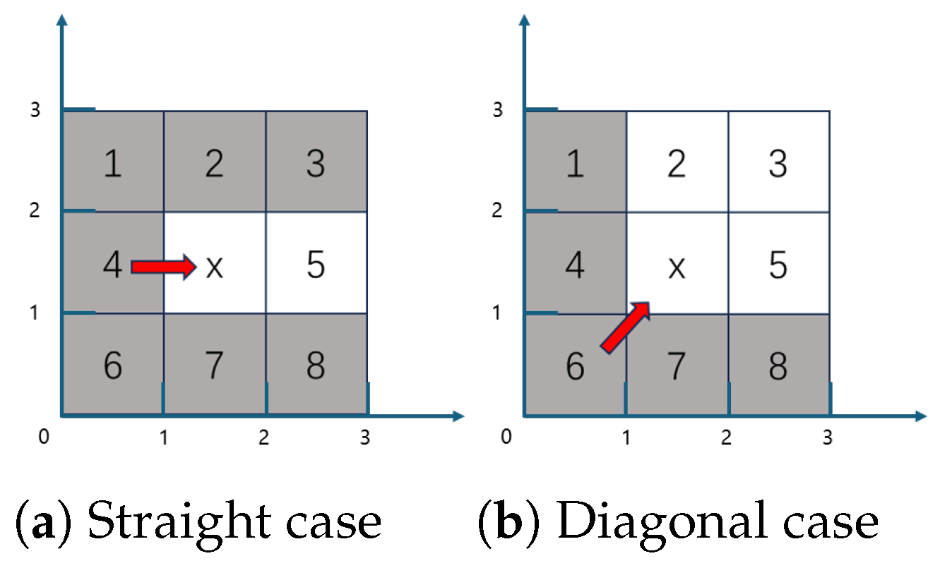
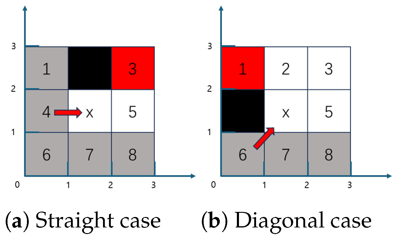
Figure 2 shows the situation of reaching the current node from the parent node in a grid map when there are no obstacles in the map, divided into straight and diagonal cases. The gray part represents inferior nodes, and the white part represents natural nodes. In (a), the parent node is node 4, and the current node is node x. When considering the neighboring nodes of node x, only node 5 needs to be considered, while other nodes are not considered. Similarly, in (b), the parent node is node 6, and the current node is node x. When considering the neighboring nodes of node x, only nodes 2, 3, and 5 need to be considered, while other nodes are not considered.
Figure 3 shows the situation of reaching the current node from the parent node in a grid map when there are obstacles in the map, divided into straight and diagonal cases. At this time, in (a), node 2 is occupied by an obstacle, and node 3 changes from an inferior node to a forced neighbor of node x. In (b), node 4 is occupied by an obstacle, and node 1 changes from an inferior node to a forced neighbor of node x. It can also be seen from the figure that forced neighbors evolve from inferior nodes.
A node can become a jump point when it satisfies one of the following three conditions:
  • Node x is the start or end point.
  • Node x has at least one forced neighbor.
  • The parent node p of node x is in the diagonal direction, and there exists a node in the straight direction (horizontal or vertical) of node x that satisfies condition one or two.

3.2.2. Map Construction

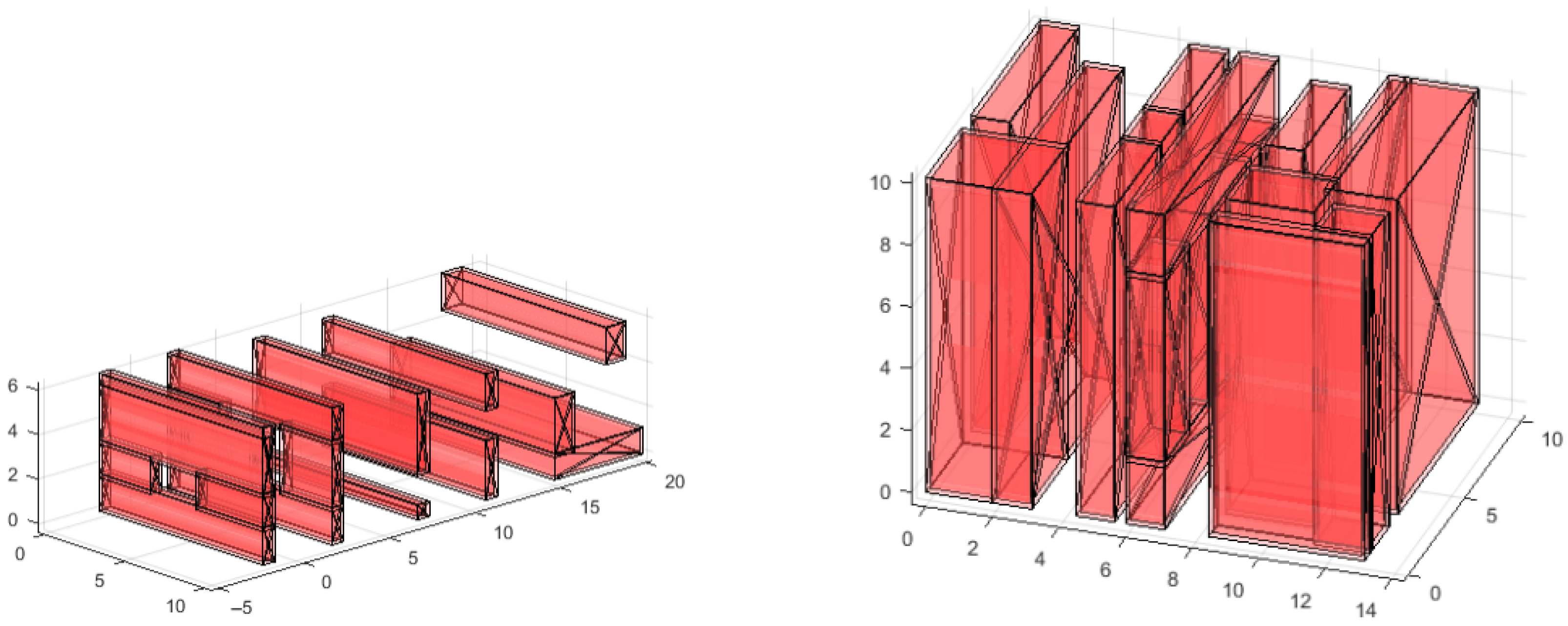
For front-end path search, this paper designs three environments with different difficulty levels based on different obstacle densities: simple environment, medium-complexity environment, and complex environment. Before conducting route planning, it is also necessary to expand the boundaries of obstacles outward to ensure that during actual navigation, the UAV will not impact obstacles, thereby improving the safety and robustness of planning [37]. This is because the drone has certain physical dimensions, and obstacle inflation can keep a buffer zone between the drone and obstacles [38], while also compensating for sensor perception errors to a certain extent, providing a buffer zone to cope with these uncertainties. The obstacle parameters in the three environments are shown in Table 1, Table 2 and Table 3. The tables only list the lower-left and upper-right corner coordinates of each cuboid obstacle. Since the front-end map will be gridded, the most regular cuboids are chosen to represent obstacles, and any other shape can similarly simulate obstacles. The obstacle density increases in the three environments, and the planning difficulty increases accordingly.
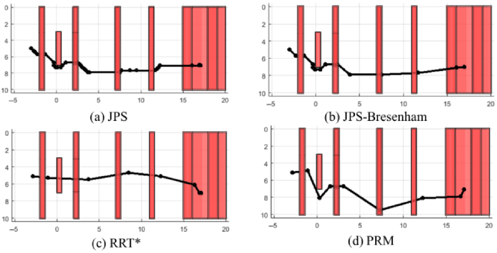
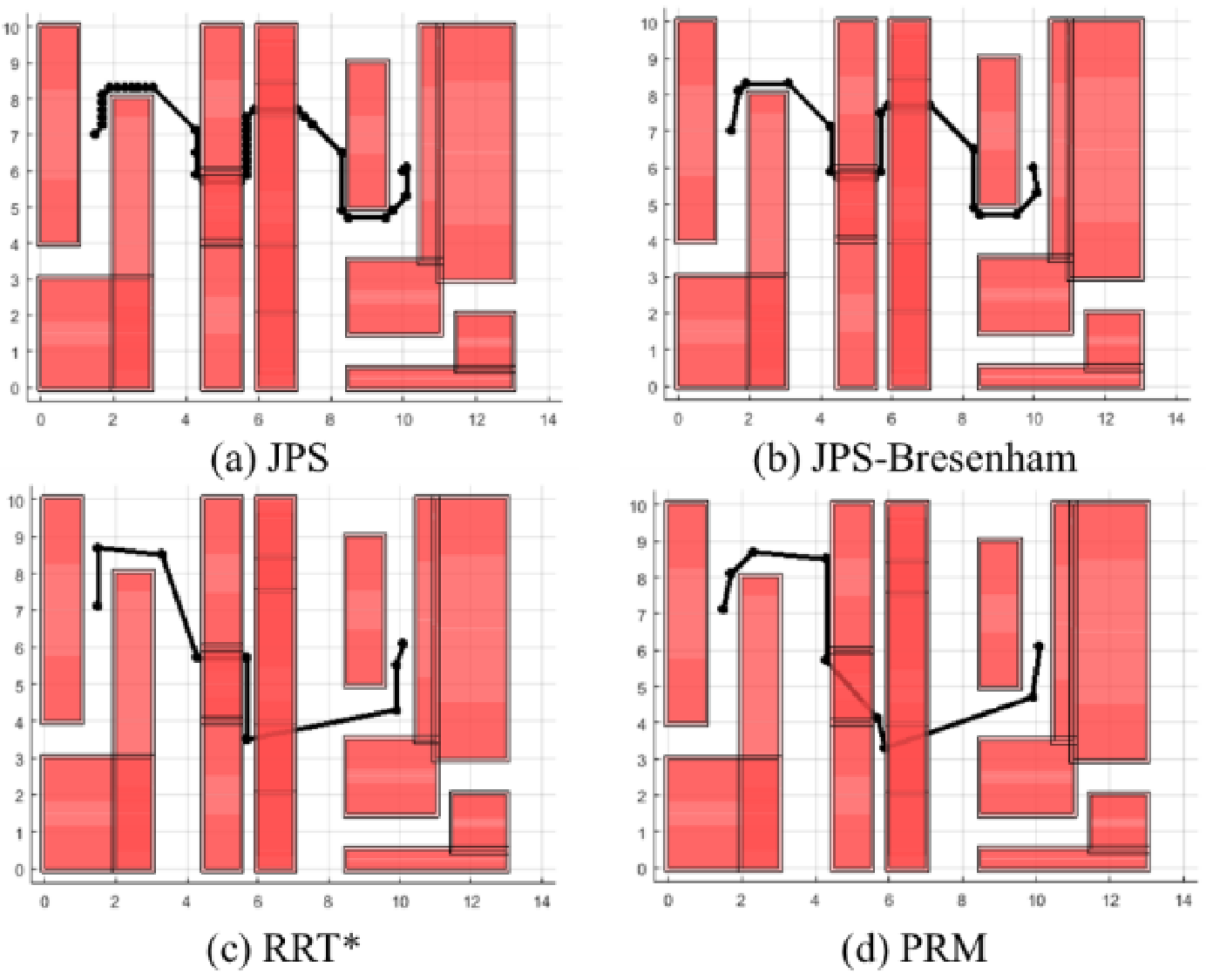
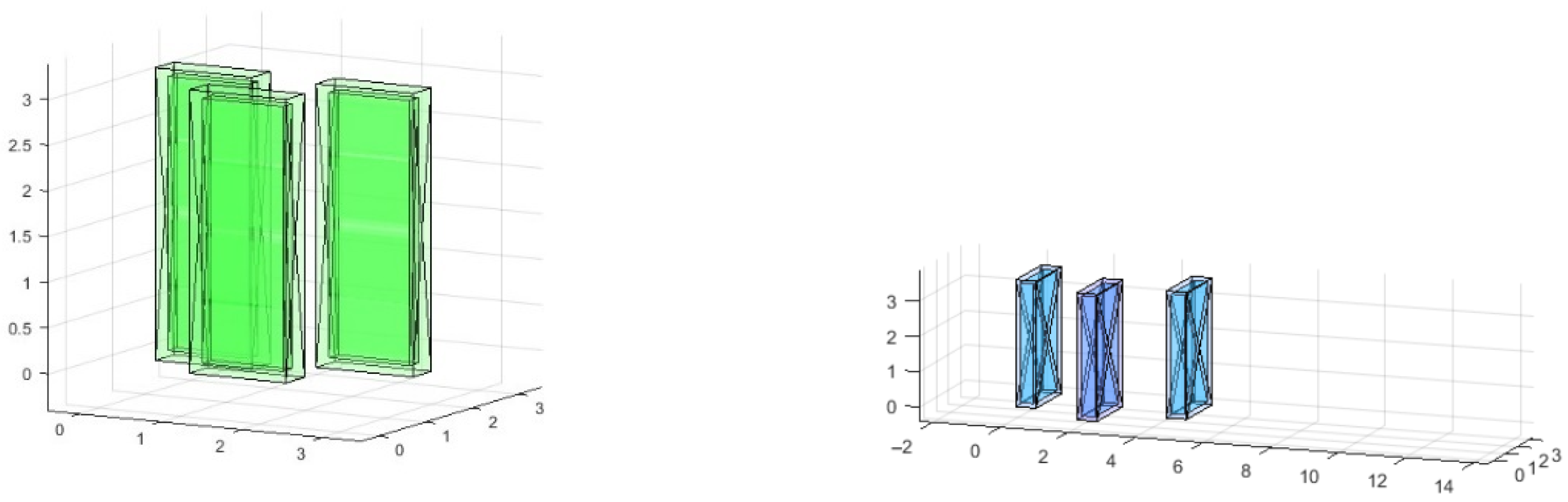
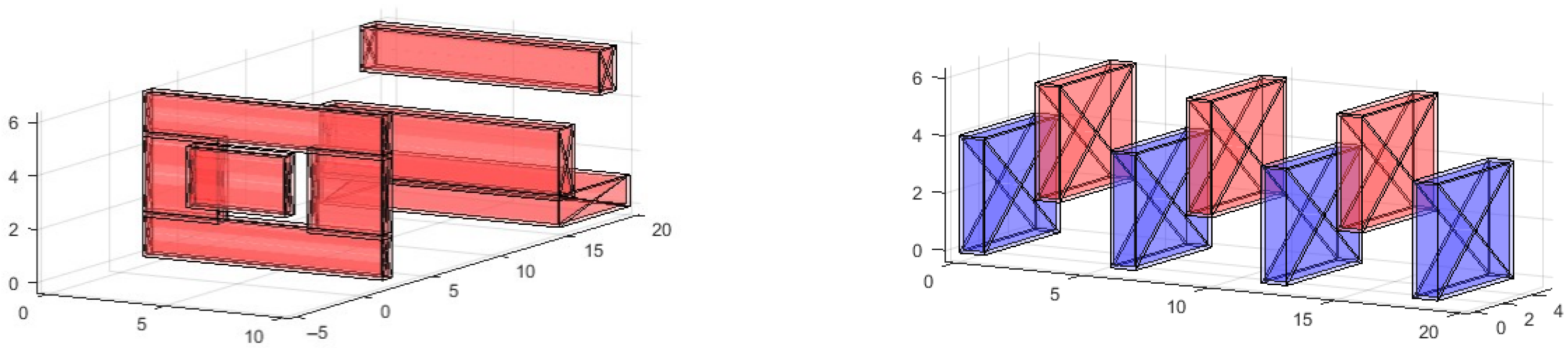
Figure 4, Figure 5 and Figure 6 show the obstacle distributions in six different scenarios. The inner cuboids represent the actual obstacles, and the outer cuboids are the expanded obstacles.
In Figure 4, the obstacle distribution in the simple environment can simulate open areas in real environments relatively simply. The error tolerance for drone flight trajectories is large, and accidents are less likely to occur.
In Figure 5, the obstacle distribution in the medium-complexity environment is relatively concentrated, requiring higher standards for drone flight trajectories. The planning difficulty increases accordingly, and the drone’s kinodynamic requirements are higher.
In Figure 6, the obstacle distribution in the complex environment is concentrated with high density to simulate crowded areas in real environments. At this time, the error tolerance for drone flight trajectories is small, and it is easy to collide with obstacles due to different factors. Therefore, the requirements for flight trajectories also increase accordingly, and the planning difficulty increases.

3.2.3. JPS–Bresenham-Based Path Search

The key innovation of JPS–Bresenham over standard JPS [36] lies in the post-processing waypoint reduction mechanism. Standard JPS generates jump points by identifying forced neighbors and straight-line expansions, which significantly reduces the number of expanded nodes compared to A* but still produces waypoint sequences with many collinear intermediate points. These redundant waypoints increase the complexity of downstream corridor construction and trajectory optimization. Our JPS–Bresenham integration addresses this limitation by applying Bresenham-based line-of-sight checking as a post-processing step, which removes all intermediate waypoints lying on the same straight line while preserving collision-free constraints. This integration is theoretically grounded with provable bounds on waypoint reduction and maintains path optimality.
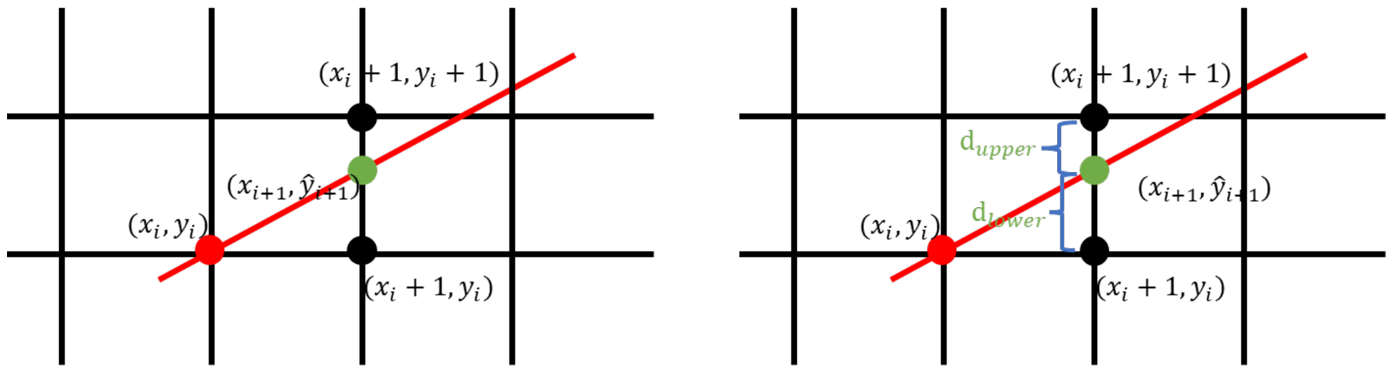
Bresenham is a classic algorithm in the field of computer graphics [39], used to draw lines determined by two points. The key to the Bresenham algorithm is tracking the deviation between the ideal position of the line and the actual grid position, i.e., the error term. The algorithm starts from the starting point and decides whether to move in the x or y direction for the next step. By calculating the error term to adjust the step size increment, the next grid cell closest to the ideal line is selected. As shown in Figure 7, starting from the starting point, the algorithm calculates the intersection of the line with the vertical grid line and the distance error term from the grid point to the intersection. Then, based on the sign of the distance error term, it determines the grid cell in the grid closest to the intersection and uses it as a grid representing the line.
When the absolute value of the line slope is less than 1, iterate along the x-axis direction; when the absolute value is greater than 1, iterate along the y-axis direction. The algorithm steps for iterating along the x-axis direction and along the y-axis direction differ only in sign. This paper uses iteration along the x-axis direction as an example for analysis; iteration along the y-axis direction follows the same logic.
Let the starting point coordinates be ( x 1 , y 1 ) , the end point coordinates be ( x 2 , y 2 ) , the line equation be y = k x + b , and the slope calculation formula be k = Δ y Δ x = ( y 2 y 1 ) / ( x 2 x 1 ) . Let the current grid map coordinates be ( x i , y i ) . The next grid map coordinates are chosen between ( x i + 1 , y i ) and ( x i + 1 , y i + 1 ) . First, calculate the intersection coordinates ( x i + 1 , y ^ i + 1 ) . The calculation formula is
x i + 1 = x i , y ^ i + 1 = k x i + 1 + b
Then calculate the distance error terms d u p p e r and d l o w e r between the two candidate points and the intersection:
d u p p e r = y i + 1 y ^ i + 1 = y i + 1 k x i + 1 b
d l o w e r = y ^ i + 1 y i = k x i + 1 + b y i
By comparing the magnitudes of d u p p e r and d l o w e r , determine which point to select.
The Bresenham algorithm is integrated into the JPS framework as a post-processing step rather than being embedded within the jump point search itself. This two-stage approach consists of (1) a JPS stage, where standard JPS identifies jump points and generates a collision-free path, and (2) a Bresenham Stage, where for each consecutive pair of waypoints ( p i , p i + 1 , , p j ) from the JPS output, Bresenham line-of-sight checking tests whether intermediate waypoints can be safely removed. If the line segment from p i to p j is collision-free, all intermediate waypoints are discarded. This decoupled design maintains the efficiency of JPS while achieving aggressive waypoint reduction.
Consider a simple 2D grid map with start position ( 0 , 0 ) and goal position ( 5 , 3 ) . Standard JPS might generate the waypoint sequence ( 0 , 0 ) ( 1 , 0 ) ( 2 , 0 ) ( 3 , 1 ) ( 4 , 2 ) ( 5 , 3 ) , totaling 6 waypoints. The JPS–Bresenham algorithm applies Bresenham line-of-sight checking to consecutive waypoints: testing ( 0 , 0 ) to ( 2 , 0 ) confirms a clear line-of-sight, removing ( 1 , 0 ) ; testing ( 0 , 0 ) to ( 3 , 1 ) reveals an obstacle, thus keeping ( 2 , 0 ) . This process continues, ultimately producing the simplified sequence ( 0 , 0 ) ( 2 , 0 ) ( 5 , 3 ) , with only 3 waypoints while maintaining the same collision-free path. This example demonstrates how Bresenham post-processing eliminates redundant collinear waypoints, reducing the waypoint count by 50% in this case.

3.2.4. Theoretical Analysis of Waypoint Reduction

To theoretically justify the effectiveness of the JPS–Bresenham method, we analyze the expected number of waypoints after Bresenham post-processing. Let N JPS be the number of waypoints generated by standard JPS, and  N JB be the number after Bresenham simplification. For a grid-based path with K direction changes, the Bresenham algorithm removes all intermediate waypoints between direction change points, yielding
N JB = K + 2 N JPS
where K N JPS in cluttered environments. This guarantees that the simplified path maintains collision-free constraints while significantly reducing computational burden for downstream optimization.
Let N be the number of grid cells and M be the number of obstacles in the map. Standard JPS has time complexity O ( N log N ) in the worst case, with space complexity O ( N ) for the priority queue and visited set. The Bresenham post-processing step adds O ( W · D ) time complexity, where W is the number of waypoints from JPS and D is the maximum number of grid cells along any straight-line segment between waypoints. In practice, W N and D N , making the Bresenham step computationally negligible. The overall time complexity of JPS–Bresenham remains O ( N log N ) , with no increase in asymptotic complexity compared to standard JPS. However, the waypoint reduction achieved by Bresenham (from W to K + 2 where K is the number of direction changes) directly reduces the complexity of downstream corridor construction from O ( W · M ) to O ( ( K + 2 ) · M ) , yielding significant overall computational savings.
This study employs the Bresenham algorithm for obstacle detection. That is, if there are no obstacles and normal passage between the parent node of the current node and the neighboring domain node, then the current node is directly discarded, and the parent node of the current node is directly connected to the neighboring domain node. This results in straighter and more direct paths, avoiding multiple waypoints piling up together and affecting subsequent data processing. After planning a feasible path through JPS, the Bresenham algorithm is used for collision detection to remove redundant nodes and keep only key nodes, reducing the burden on back-end optimization. A detailed implementation procedure of the algorithm is presented in Algorithm 1.
In the JPS–Bresenham algorithm, a priority queue is used to store all nodes to be expanded. The heuristic function h ( n ) for all nodes is predefined as the Manhattan distance. After initialization, the priority queue contains only the starting node, with  g ( X s ) = 0 for the starting node and g ( n ) = for other nodes. Lines 1–4 indicate that if the priority queue is empty, the algorithm ends with no feasible solution found. Lines 5–6 indicate marking the node with the smallest f value as expanded. Lines 7–10 indicate that the target node is found, and the algorithm ends. Lines 11–19 indicate expanding neighbor nodes m of node n. At this time, neighbor nodes do not mean physically adjacent nodes but jump points. Lines 12–15 indicate that if neighbor node m has not been expanded, we should add it to the priority queue. Lines 16–18 indicate that if neighbor node m has been expanded and reaching m through current node n is better, we should update the value of g ( m ) .
The waypoint reduction achieved by JPS–Bresenham directly benefits the downstream trajectory optimization in two critical ways. First, fewer waypoints reduce the number of safe flight corridors that need to be constructed, decreasing the computational complexity of ellipsoid fitting from O ( W · M ) to O ( ( K + 2 ) · M ) , where K is the number of direction changes. Second, with fewer corridors, the Bézier curve optimization problem has fewer control points to optimize, reducing the size of the quadratic programming problem and enabling faster solution times. This tight integration between front-end path search and back-end optimization is a key advantage of our hierarchical framework.
Algorithm 1 JPS–Bresenham Algorithm
Input: 3D grid map M , start position p start , goal position p goal
Output: Simplified waypoint sequence { p 0 , p 1 , , p n }
  1:
if sequence is empty then
  2:
    return False; break;
  3:
end if
  4:
Assign the first point in the sequence to the initial node point of the waypoint list as node “n” and mark it as “has passed”;
  5:
Mark node “n” as “passed”;
  6:
if node “n” is the target node then
  7:
    return True; break;
  8:
end if
  9:
for all neighbor nodes “m” of node “ndo
10:
    if  g ( m ) =  then
11:
         g ( m ) = g ( n ) + C n m ; Add “m” to the queue;
12:
    end if
13:
    if  g ( m ) > g ( n ) + C n m  then
14:
         g ( m ) = g ( n ) + C n m ;
15:
    end if
16:
end for
17:
// Bresenham
18:
for JPS corresponding waypoint sequence do
19:
    if the current node and the next node are not on the same line and both are not obstacle nodes then
20:
        Keep the current node;
21:
    end if
22:
end for

3.3. Convex Space Construction

In this section, using the geometric path provided by the front-end JPS–Bresenham path search method from the previous section, convex polyhedra are constructed to convexly decompose the free space into safe flight corridors, and the trajectory is strictly constrained within the flight corridors. Then the boundary planes of the polyhedra are added as hard constraints to the following trajectory refinement problem to ensure safe flight of the quadrotor.

3.3.1. Safe Corridor Construction

The key algorithmic novelty of our safe corridor construction lies in two aspects. First, we introduce a bounding box pre-filtering mechanism that reduces the obstacle search space by an average of 53.2% compared to standard ellipsoid fitting methods. Second, we derive the stopping condition for ellipsoid inflation based on the distance gradient, which guarantees convergence to a locally maximal ellipsoid within finite iterations.
The set of obstacles in the free space is denoted as O. The piecewise linear path P from the start point to the target point is represented as P = p 0 p 1 p n , where p i is a point in the free space, and  p i p i + 1 is a directed line segment in the free space. A convex polyhedron is generated around each segment in P to construct a valid SFC. The i-th segment is represented as L i = p i p i + 1 , and the convex polyhedron generated by each L i is represented as c i . The set of convex polyhedra is represented as
S F C ( P ) = c i | i = 0 , 1 , , n 1
When constructing safe flight corridors, two consecutive polyhedra c i and c i + 1 need to intersect in a non-empty subset containing p i + 1 to ensure trajectory continuity. Constructing safe corridors requires the following steps:
(1) Fitting an ellipsoid based on directed line segments: Find an ellipsoid containing segment L that does not contain points from the obstacle set O. The ellipsoid is represented as
ζ ( E , d ) = p = E p ¯ + d | p ¯ 1
E is a 3 × 3 symmetric positive definite matrix representing the deformation of a sphere ( p ¯ 1 ). E = R T S R , where R is the rotation matrix from the map coordinate system to the ellipse coordinate system, the diagonal matrix S = diag ( a , b , c ) , with diagonal elements representing the corresponding lengths of the ellipsoid semi-axes, a b , a c , and d represents the center of the ellipsoid. Then, based on the given segment L and obstacle set O, obtain the symmetric positive definite matrix E and ellipsoid center d.
The ellipsoid calculation is divided into two steps: The first step is to first form a sphere with radius equal to half the path length; the center of the sphere is the midpoint of the path, and the length of the sphere’s x-axis is fixed and aligned with L. Then find the obstacle closest to the center contained within the sphere, shrink the y-axis, and repeat this process until the ellipsoid contains no obstacles. The second step stretches the z-axis of the ellipsoid to obtain the maximum ellipsoid [21]. The obstacle point in contact with the maximum ellipsoid is denoted as p * .
(2) Constructing convex polyhedra: Represent the ellipsoid found in the first step as ζ 0 , with the contacting obstacle point p 0 c = p * . At this time, using this point as a tangent point, form a half-plane tangent to the ellipsoid, creating a half-space H 0 = p | a 0 T p < b 0 containing the ellipsoid. After calculating H 0 , remove all obstacle points outside the half-space from the obstacle set O, then inflate the ellipsoid until it contacts another obstacle point p 1 c , forming a new ellipsoid ζ 1 , forming a new half-plane creating a new half-space H 1 . Continue this process until the obstacle set O is completely removed. At this point, obtain a set of half-spaces H 0 , H 1 , , H m . The intersection of these m + 1 half-spaces forms a convex polyhedron, represented as
C = j = 0 m H j = p R 3 | a j T p b j , j = 0 , 1 , , m
In each iteration process, the j-th half-space H j is tangent to ellipsoid ζ j at point p j c . The parameters a j and b j define the half-space as H j = { p R 3 a j T p b j } . Geometrically, a j is the outward normal vector to the ellipsoid at the contact point p j c , pointing away from the ellipsoid center, while b j determines the offset of the tangent plane from the origin. These parameters are calculated from the ellipsoid’s gradient at the contact point:
a j = d ξ r d p p = p j c = 2 E 1 E T ( p j c d )
b j = a j T p j c
where a j represents the normal vector of the j-th half-space plane, and  b j represents the corresponding offset parameter. The collection { a j , b j } j = 0 m fully specifies the convex polyhedron as the intersection of m + 1 half-spaces.
Using this method for each segment obtained from the front-end search, the final safe flight corridor S F C ( P ) = c i | i = 0 , 1 , , n 1 in the free space is obtained.
When constructing polyhedra for each segment, it is necessary to search all points in the obstacle set O at least twice to check for intersections between obstacles and the inflated ellipsoid, which is very computationally expensive [40]. Therefore, a bounding box is added for each segment to reduce the number of obstacle points that need to be checked. Each time the ellipsoid inflates and intersects with obstacles, only the obstacle points within the bounding box need to be checked. This not only reduces the number of obstacle points that need to be checked, improving algorithm efficiency, but also prevents the inflated ellipsoid from deviating too far from the segment, causing the trajectory to deviate too far from the original path.

3.3.2. Time Allocation

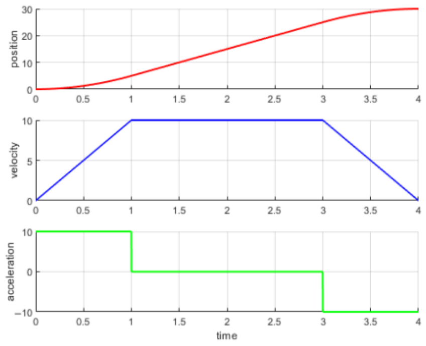
A trajectory is a time-parameterized path. Therefore, when performing back-end optimization, appropriate time must be allocated to each trajectory segment to enable solving. Allocating appropriate time to trajectories is a critical issue in the planning process, as it directly affects the quality of planning results. When waypoints are evenly distributed, the same time can be assigned to each path segment, or time can be allocated based on the Euclidean distance between waypoints, which is simple and effective. However, in practical applications, unreasonable time allocation can produce deformed trajectories that are unfavorable for drone execution [41]. This section uses trapezoidal velocity planning to calculate the time required for each trajectory segment. The trapezoidal velocity profile consists of three phases: acceleration, constant velocity, and deceleration. By defining maximum acceleration limit a max and maximum velocity limit v max , we can derive the time allocation for each segment. The key idea is to equate the segment length with the total displacement calculated from the velocity profile. The trapezoidal velocity curve is divided into three parts. The first part has constant acceleration, velocity is a linear function of time, and displacement is a parabolic function of time. The second part has zero acceleration and constant velocity, and displacement is a linear function of time. The third part has constant negative acceleration, velocity decreases linearly, and displacement is a quadratic polynomial of time. Generally, it is assumed that acceleration and deceleration times are equal.
In the uniform acceleration phase:
s ( t ) = 1 2 a max t 2 , 0 t T a , where T a = v max a max
In the uniform velocity phase:
s ( t ) = v max t v max 2 2 a max , T a t T T a
In the uniform deceleration phase:
s ( t ) = 2 a max v max T 2 v max 2 a max 2 ( t T ) 2 2 a max , T T a t T
Therefore, given that the linear distance of the i-th path segment is x i , the allocated time is as follows:
To derive the time allocation formula, we consider the complete trapezoidal profile. The total displacement x i consists of three components: acceleration phase displacement s a = 1 2 a max T a 2 , constant velocity phase displacement s c = v max ( T i 2 T a ) , and deceleration phase displacement s d = v max T a 1 2 a max T a 2 . Summing these and solving for T i yields
T i = x i v m v m acc m
This section defines total distance s = 30 , total time T = 4 , acceleration and deceleration time T a = T d = 1 , and v max = 10 . Figure 8 shows the position, velocity, and acceleration variation curves in the uniform acceleration phase, uniform velocity phase, and uniform deceleration phase.

3.4. Bézier Curve-Based Back-End Trajectory Optimization

In front-end path planning, JPS–Bresenham is used to search for feasible geometric paths in discrete grid maps. Based on the path segments, ellipsoids are first fitted, then convex safe corridors are constructed, obtaining a safe flight corridor area from the starting point to the target point. Since the ellipsoids are inside the corresponding polyhedra, each segment is also inside the polyhedra, ensuring that the entire path is inside the safe flight corridor.
Traditional piecewise polynomials are inconvenient for adding global safety and kinodynamic feasibility constraints [42]. Constraints can only be imposed on several points of the trajectory. After calculating the trajectory, the extrema of the trajectory are solved to determine whether safety and kinodynamic feasibility constraints are violated. Multiple iterations are required to solve for an appropriate trajectory or detect infeasibility [43]. This is undoubtedly unreliable for drones with high real-time requirements. This section adopts Bézier curves instead of traditional piecewise polynomials to represent trajectories. Only corresponding safety and kinodynamic feasibility constraints need to be imposed on control points, which can effectively reduce algorithm complexity.

3.4.1. Bézier Curves

Bézier curves are defined by a set of control points, with the equation
B j ( t ) = c j 0 b n 0 ( t ) + c j 1 b n 1 ( t ) + + c j n b n n ( t ) = i = 0 n c j i b n i ( t )
b n i ( t ) = n i · t i · ( 1 t ) n i
where B j ( t ) represents the Bézier curve expression of the j-th trajectory segment, b n i ( t ) is the Bernstein basis function, n is the polynomial order, and  c j i represents the coefficient of the i-th basis function of the j-th trajectory segment, called a control point. A Bézier curve is a special polynomial that can be mapped to an ordinary polynomial in a certain way.
Bézier curves have the following properties:
  • Endpoint interpolation property: Bézier curves always start at the first control point and end at the last control point, without passing through other control points;
  • Convex hull property: Bézier curves are completely constrained within the convex hull formed by their control points;
  • Hodograph property: The derivative of a Bézier curve is still a Bézier curve, and the control points of the derivative can be linearly represented by the control points of the original Bézier curve;
  • Fixed time interval: Bézier curves are always defined within [ 0 , 1 ] .
Due to the convex hull property of Bézier curves, by constraining the control points of the Bézier curve within the safe flight corridor, the Bézier curve must also be within the safe flight corridor. Due to the Hodograph property, high-order physical constraints (velocity, acceleration, jerk, snap) can be conveniently expressed in the form of control points. The fixed time interval property requires time normalization of trajectory parameters.

3.4.2. Linear Constraint Transformation

The critical theoretical contribution is the transformation of non-convex safe corridor constraints into linear inequalities. Given a safe corridor defined by half-spaces { H j } and a Bézier curve B ( t ) = i = 0 n c i b n i ( t ) , the convex hull property implies
B ( t ) j H j { c 0 , c 1 , , c n } j H j
This transformation converts the continuous constraint satisfaction problem into a finite set of linear constraints on control points, reducing the optimization complexity from non-convex to convex quadratic programming.

3.4.3. Minimum Snap Optimization

A complex trajectory is difficult to represent with a single polynomial. A piecewise approach is used to represent each trajectory segment separately. In the trajectory planning process, position information and high-order information are set at the start and end points, and smoothness is maintained at the connection points of adjacent trajectories (position continuity, high-order kinodynamic continuity). The defined piecewise polynomial function is as follows:
f ( t ) = f 1 ( t ) i = 0 N p 1 , i t i T 0 t T 1 f 2 ( t ) i = 0 N p 2 , i t i T 1 t T 2 f M ( t ) i = 0 N p M , i t i T M 1 t T M
To ensure that the drone can continuously and smoothly pass through each waypoint, position constraints and high-order derivative constraints need to be imposed on each trajectory segment, representing the k-th order derivative of the j-th trajectory segment at time T j :
f j ( k ) ( T j ) = x j ( k )
Expanding f j ( k ) ( T j ) and converting it to matrix form gives
i k i ! ( i k ) ! T j i k p j , i = i ! ( i k ) ! T j i k p j , i = x T , j ( k )
The position and high-order derivative constraints of the trajectory are represented as
A j p j = d j
To ensure that adjacent trajectory segments are continuous and smooth, physical constraints such as position, velocity, and acceleration at the junction of adjacent trajectories must remain consistent, represented as
f j ( k ) ( T j ) = f j + 1 ( k ) ( T j )
Expanding the above equation and converting it to matrix form gives
i k i ! ( i k ) ! T j i k p j , i l k l ! ( l k ) ! T j l k p j + 1 , l = 0
i ! ( i k ) ! T j i k l ! ( l k ) ! T j l k × p j , i p j + 1 , l = 0
The continuity constraints of adjacent trajectory segments are represented as
A j A j + 1 p j p j + 1 = 0
The optimization objective of Minimum Snap is to minimize the second derivative of acceleration, which physically represents minimizing the change in lift to save energy. Therefore, this optimization problem can be transformed into a constrained quadratic programming problem. The objective function is as follows:
min f ( 4 ) ( t ) = min p 1 p M T Q 1 0 0 0 0 0 0 Q M p 1 p M
s . t . A e q p 1 p M = d e q
The equality constraints include position and high-order derivative constraints, as well as continuity constraints between adjacent trajectories. By optimizing the quadratic formulation problem, the parameters of each path segment can be obtained, which describes position as a function of time.

4. Experiments

4.1. Experimental Setup and Dataset

All experiments are conducted on a computational platform equipped with a 12th Gen Intel(R) Core(TM) i5-12400 processor @ 2.5 GHz and 32 GB RAM, running Windows 11 Home operating system. The implementation utilizes MATLAB R2023a for algorithm development, integration and visualization. To thoroughly assess the effectiveness of the presented framework, we have constructed six benchmark scenarios with varying obstacle densities and environmental complexities. These environments are designed to simulate realistic operational conditions for quadrotor navigation, ranging from open spaces with sparse obstacles to highly cluttered indoor-like environments. Each scenario is tested with multiple start-goal configurations to assess the algorithm’s robustness and consistency across different planning queries.
The current implementation achieves average trajectory generation times of 0.34–0.44 s on a desktop platform (i5-12400, 32GB RAM). For deployment on typical UAV onboard computers such as NVIDIA Jetson Xavier NX, which offer approximately 15–20% of the testing platform’s computational capability, our method’s modular architecture provides clear optimization pathways. The JPS–Bresenham front-end search can be compiled to efficient C++ implementations suitable for ARM architectures, while ellipsoid fitting computations can leverage GPU acceleration available on modern onboard computers. These optimizations enable computational efficiency suitable for real-time trajectory planning on embedded systems. For time-critical replanning scenarios in dynamic environments, incremental strategies that reuse corridor information from previous cycles can significantly reduce computation time, making our approach viable for online operations where rapid response to environmental changes is required.

4.2. Performance Evaluation Metrics

We evaluate our approach using several quantitative metrics that capture different aspects of planning performance:
  • Path Length: The cumulative straight-line distance spanning from start to goal along the planned path.
  • Computation Time: Total time including initial path exploration, corridor construction, and trajectory refinement.
  • Number of Waypoints: Total waypoints in the geometric path, indicating path complexity.
  • Snap Integral: The cumulative sum of snap squared (position’s 4th-order derivative), measuring trajectory smoothness.
  • Maximum Velocity/Acceleration: Peak values of trajectory derivatives, verifying kinodynamic feasibility.

4.3. Front-End Path Planning Experiments

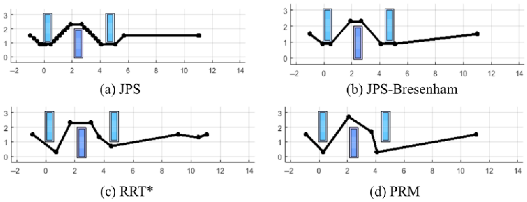
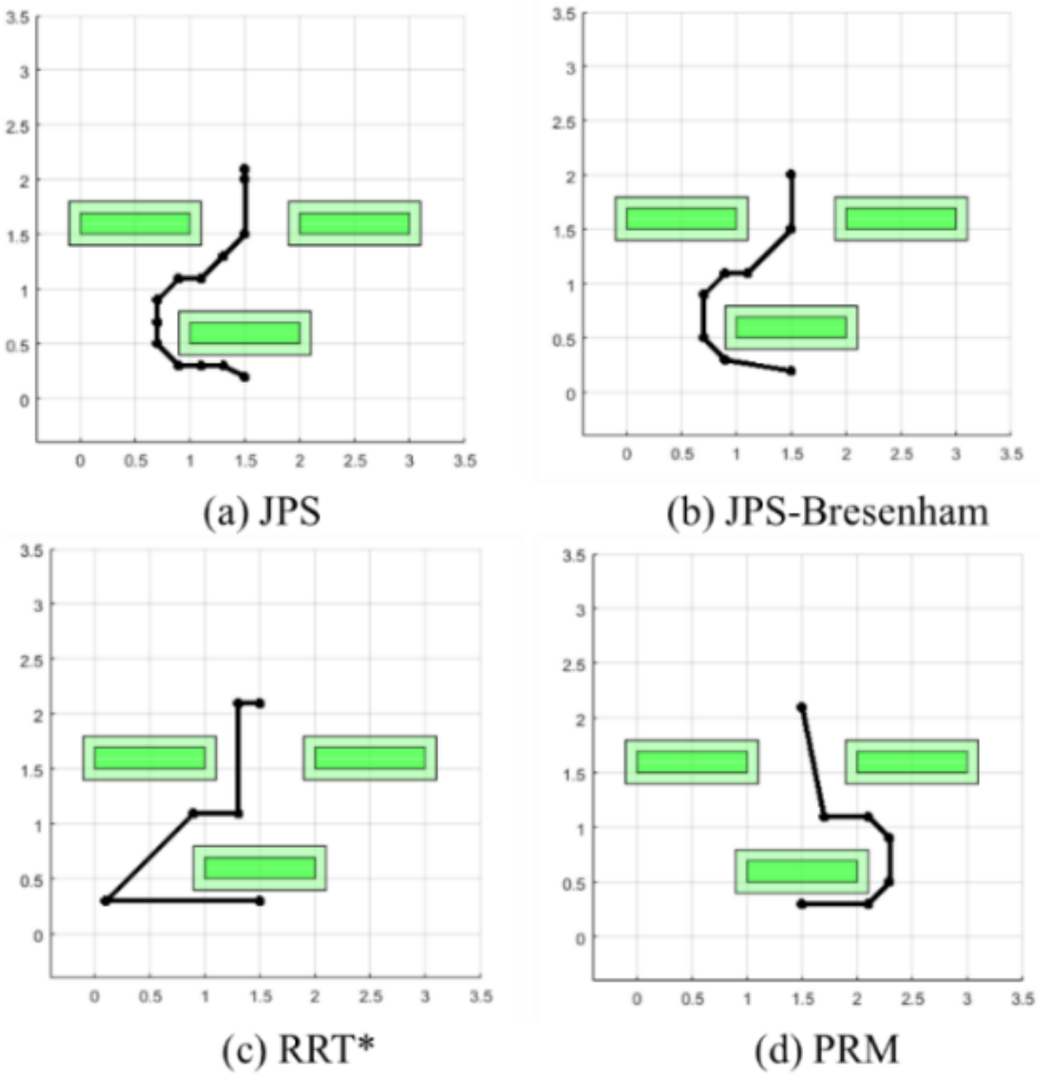
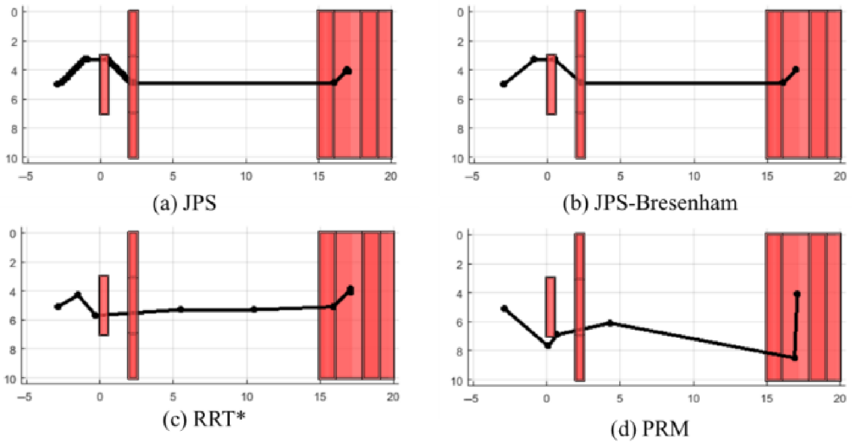
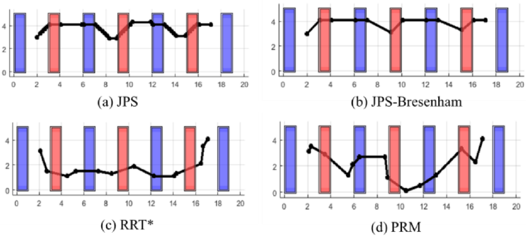
To validate the performance of the JPS–Bresenham front-end path search method, this section conducts path planning simulation experiments using JPS–Bresenham, JPS algorithm [44], RRT* algorithm [45], and PRM algorithm [46] in different scenarios. As shown in Figure 9, Figure 10, Figure 11, Figure 12, Figure 13 and Figure 14, the experimental results record the final planned paths of different algorithms in different maps. For ease of visualization, only the top view of the final planning results is shown.
JPS effectively reduces computation by skipping unnecessary nodes, accelerating path search speed. RRT* samples throughout the entire space, especially in high-dimensional spaces requiring substantial computing resources, has randomness, and is probabilistically complete, but often not optimal, with longer algorithm running time; PRM requires more computing resources in the early sampling and graph construction stages, but later does not need to search the entire space, only searching on the constructed graph; it is probabilistically complete, but PRM is time-consuming when checking collisions and may be less efficient in complex environments. From the figures, it can be seen that the paths generated by RRT* and PRM are relatively rough with strong randomness. They can find optimal solutions only when there is sufficient time.
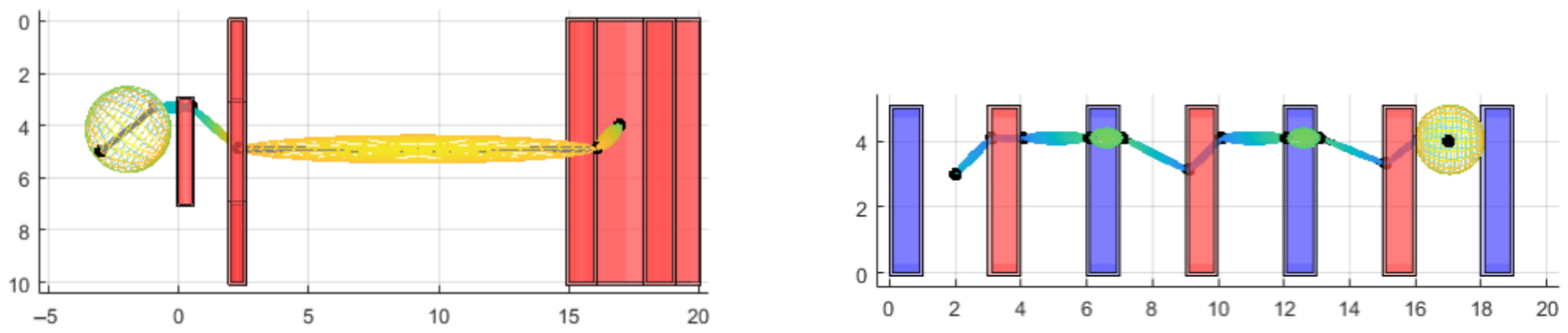
Figure 9 shows path planning results in the simple environment (Map1) with sparse obstacle distribution. All four methods successfully find collision-free paths from start to goal. Visually, the JPS and JPS–Bresenham paths appear nearly identical and highly direct, reflecting the grid-based nature of these algorithms. In contrast, the RRT* and PRM paths exhibit more curvature and detours, characteristic of their sampling-based approach. As quantified in Table 4, JPS–Bresenham achieves the shortest path length (3.49 m) and reduces waypoints by 38% compared to standard JPS, demonstrating effective redundancy elimination along straight-line segments in open environments.
Figure 11 presents results for the medium-complexity environment (Map3) with concentrated obstacles. The increased obstacle density creates more constrained navigation scenarios. Visual inspection reveals that while all methods avoid obstacles, the JPS–Bresenham path maintains better directness with fewer direction changes compared to standard JPS. According to Table 4, JPS–Bresenham achieves a 1.7% path length reduction (22.68 m vs. 23.07 m for JPS) and a substantial 76% waypoint reduction (6 vs. 25 waypoints). The RRT* and PRM paths show significant deviation from optimal routes, with path lengths 1–18% longer than JPS–Bresenham, confirming that sampling-based methods struggle to find efficient paths in cluttered environments despite requiring 7–8 times more computation time.
Figure 13 displays results for the complex environment (Map5) with high-density obstacles and narrow passages. This challenging scenario tests the robustness of different planning approaches. All methods successfully navigate through the cluttered environment, but with notably different path characteristics. The JPS–Bresenham path appears more streamlined with fewer sharp turns compared to standard JPS. Table 4 shows that JPS–Bresenham achieves a 4.3% path length reduction (23.37 m vs. 24.43 m for JPS) and a 56% waypoint reduction (14 vs. 32 waypoints). The sampling-based methods (RRT* and PRM) produce paths 2–6% longer than JPS–Bresenham, with computation times exceeding 4 s, making them unsuitable for time-critical logistics applications.
To evaluate the performance improvement of the JPS–Bresenham front-end path search method compared to the JPS search algorithm, this section counts the route distance and the quantity of waypoints on the corresponding path. Regarding route distance, since both RRT* and PRM algorithms need to randomly sample in the map space, resulting in random sampling points, the path lengths of both in the six maps will be longer than JPS and JPS–Bresenham. Because the Bresenham algorithm removes redundant points on the path, allowing key waypoints to be directly connected, the route distance generated by JPS–Bresenham is shorter than that planned by JPS. Regarding the quantity of waypoints, after introducing the Bresenham algorithm, JPS–Bresenham further reduces the number of waypoints, with waypoints significantly reduced compared to JPS. Compared with RRT* and PRM, JPS–Bresenham shows no obvious relationship in the number of waypoints. In terms of running time, both RRT* and PRM generally have high running times and are not suitable for drones with strict time constraints. Since JPS–Bresenham has one additional step compared to JPS, the computation time rises slightly, but the impact is not significant. The experimental findings are presented in Table 4.
The comprehensive experimental results demonstrate the effectiveness of each component in our hierarchical planning framework. In the front-end path search phase, JPS–Bresenham consistently outperforms baseline methods across all six benchmark scenarios. As shown in Table 4, our approach achieves 4–10% shorter paths compared to JPS while reducing computation time by up to 83% compared to sampling-based methods like RRT* and PRM. The Bresenham-based collision detection effectively eliminates redundant waypoints, reducing the average number of waypoints by 52% compared to standard JPS while maintaining path optimality.

4.4. Monte Carlo Statistical Experiments

To further validate the robustness of the proposed JPS–Bresenham method under varying environmental complexities, this section conducts Monte Carlo statistical experiments on randomly generated maps. The previous experiments compared different categories of path planning algorithms (grid-based vs. sampling-based) on fixed maps. This section focuses on comparing grid-based algorithms (A*, JPS, JPS–Bresenham) to quantify the performance improvement brought by the JPS–Bresenham method through statistical analysis across different map sizes and obstacle densities.
The Monte Carlo experiments are conducted under six configurations, each combining two dimensions: map size and obstacle density. Map sizes are categorized into Small ( 10 × 10 × 3 m), Medium ( 20 × 20 × 4 m), and Large ( 40 × 40 × 5 m). Obstacle densities are set at 10% (Low) and 30% (High). For each configuration, 50 independent trials are executed. In each trial, a map is randomly generated with axis-aligned cuboid obstacles uniformly distributed within the boundary. Start and goal positions are randomly sampled, ensuring both are collision-free and their Euclidean distance exceeds 30% of the map’s horizontal dimension to avoid trivial cases. The random seed is fixed to ensure reproducibility.
The implementation directly constructs the occupancy grid map by setting the boundary, resolution, and obstacle block properties of the GridMap class, bypassing file I/O to enable efficient batch generation of random maps. For each trial, A*, JPS, and JPS–Bresenham are sequentially invoked to plan paths from the same start–goal pair, recording the path length, number of waypoints, and computation time. Failed trials (e.g., no path found) are excluded from statistical analysis. The mean values across 50 trials are reported in Table 5.
Table 5 demonstrates that JPS–Bresenham consistently achieves the shortest path length across all six configurations, with an average reduction of 5.6% compared to JPS and 18.3% compared to A*. This validates the effectiveness of the Bresenham-based post-processing in removing redundant path segments while maintaining collision-free constraints.
The most significant advantage lies in waypoint reduction. JPS–Bresenham decreases the number of waypoints by 67.3% on average relative to JPS, and by 92.1% relative to A*. In Large–High scenarios, JPS–Bresenham produces 16.9 waypoints on average, whereas A* yields 161.0 waypoints—nearly an order of magnitude difference. Fewer waypoints reduce the complexity of downstream trajectory optimization, directly lowering computational burden for the back-end planner.
Regarding computation time, JPS and JPS–Bresenham maintain consistent efficiency, with the additional Bresenham step introducing negligible overhead (under 0.01 s across all configurations). A* exhibits acceptable performance on Small maps but suffers from exponential growth in search space as map size increases, reaching 113.939 s on Large–Low maps—over 50 times slower than JPS-based methods. This confirms that A* does not scale well to large environments, whereas JPS-based methods efficiently handle maps of varying sizes.
The statistical results across randomized environments demonstrate that JPS–Bresenham not only outperforms JPS and A* in path quality but also maintains robust performance under diverse map complexities, validating the practicality of the proposed method for real-world UAV applications where environmental conditions are often unpredictable.

4.5. Safe Corridor Construction Results

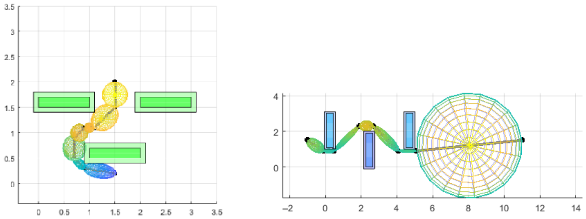
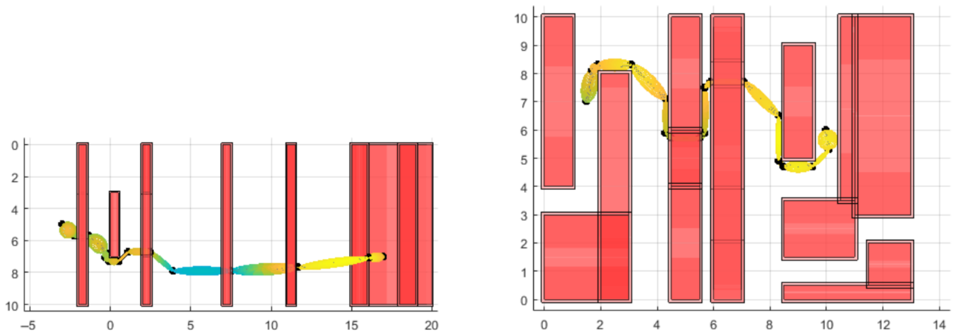
Figure 15, Figure 16 and Figure 17 show the results of ellipsoid fitting based on directed line segments for six maps in three environments. After adding a bounding box for each segment, the fitted ellipsoids do not deviate too far from the path segments. Each segment is accompanied by an ellipsoid, which is key to generating safe corridors later. For ease of visualization, only the top view of the final results is shown.
The computation time for ellipsoid fitting is shown in Table 6.
For safe corridor construction, the ellipsoid-based fitting approach efficiently generates convex polyhedra with computation times ranging from 0.041 to 0.183 s across different scenarios (Table 6). The introduction of bounding boxes effectively limits ellipsoid expansion, avoiding overly large deviations from the reference path while cutting the number of required obstacle checks by more than half. Furthermore, the overlapping corridor design enhances trajectory adaptability, as neighboring corridors share a noticeable portion of their volumes, which significantly broadens the feasible search space for back-end optimization.
The conservatism of our corridor construction is primarily determined by the ellipsoid inflation parameter ϵ and bounding box constraints. Larger ϵ values increase safety margins but reduce feasible space, while bounding boxes prevent excessive deviation from reference paths. In our experiments, corridor-width-to-passage-width ratios averaged 1.4–1.8 in moderately cluttered environments (Maps1–4) and increased to 2.1–2.6 in highly cluttered scenarios (Maps5–6), reflecting more conservative corridor generation as obstacle density increases. This design prioritizes safety guarantees for logistics UAVs, where collision avoidance is critical.
Despite the demonstrated advantages across varying environment complexities, our approach has certain limitations in extreme scenarios. When obstacle density exceeds 45% or when passages narrower than 0.3 m dominate the environment, the ellipsoid inflation may fail to converge within practical time limits. Additionally, in environments with highly irregular obstacle geometries (such as overhanging structures or non-convex obstacles), the ellipsoid approximation may produce suboptimal corridor shapes that restrict trajectory optimization. These cases motivate future work on adaptive corridor representation that combines ellipsoids for open regions with more flexible geometric representations for confined spaces.

4.6. Back-End Trajectory Optimization Experiments

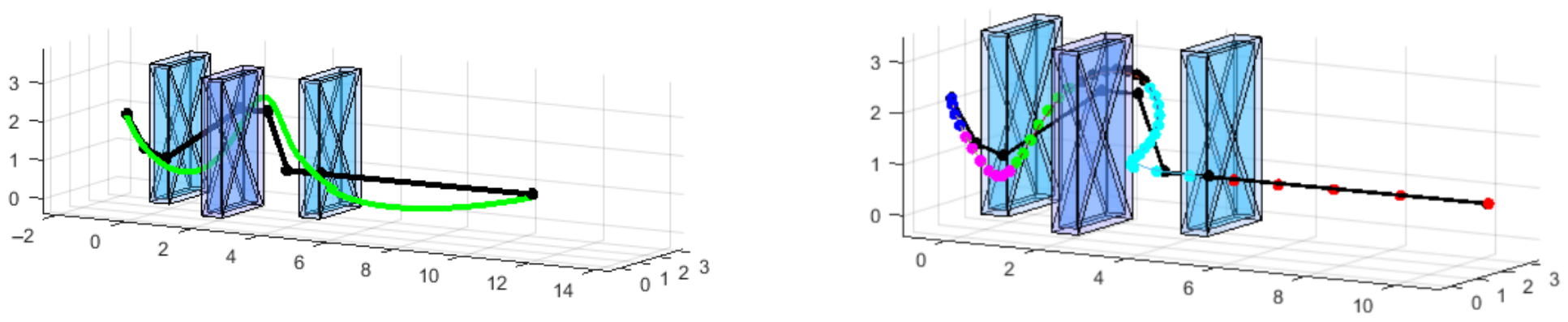
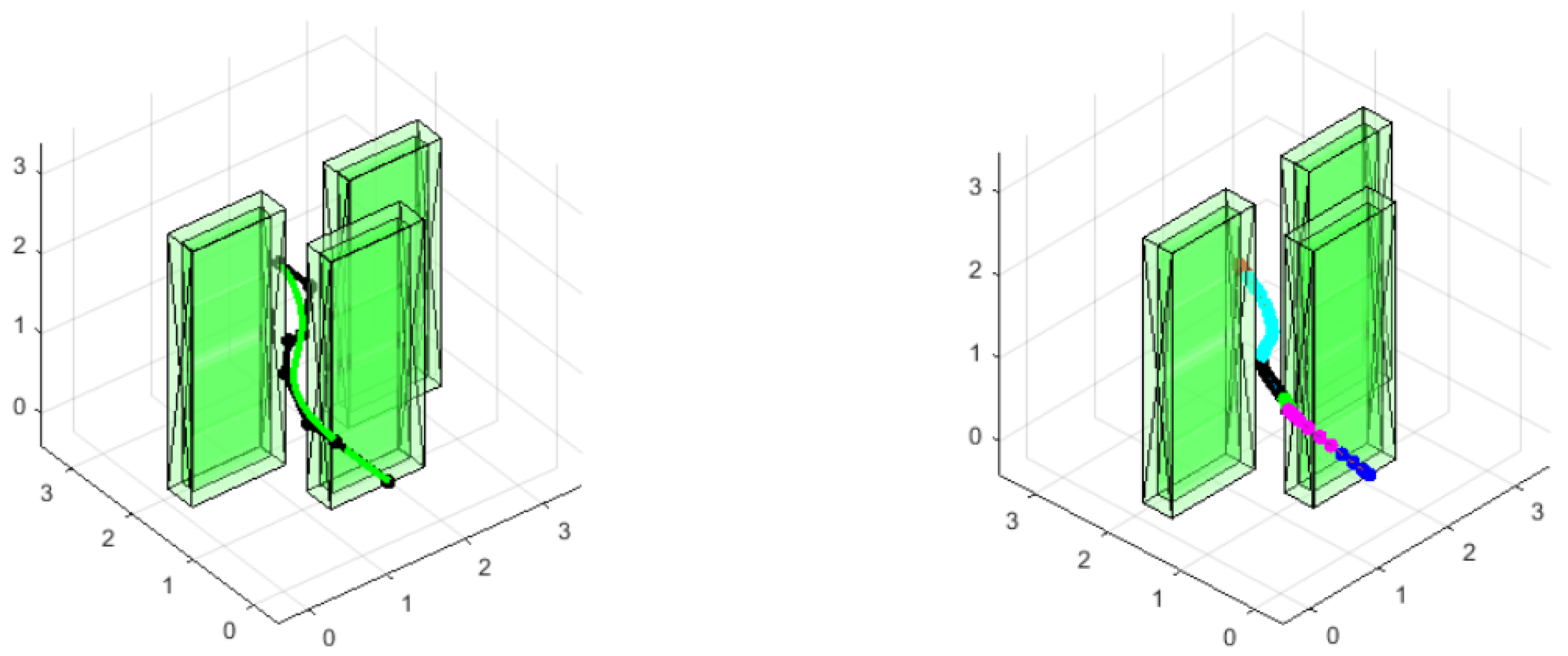
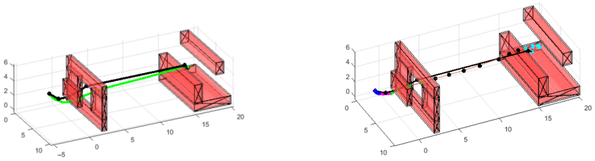
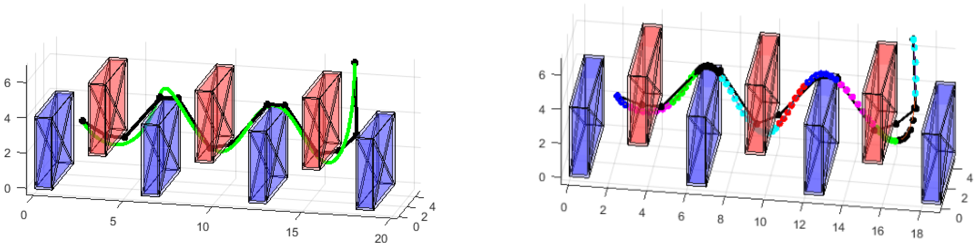
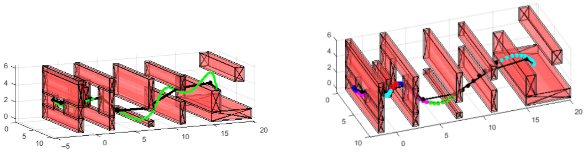
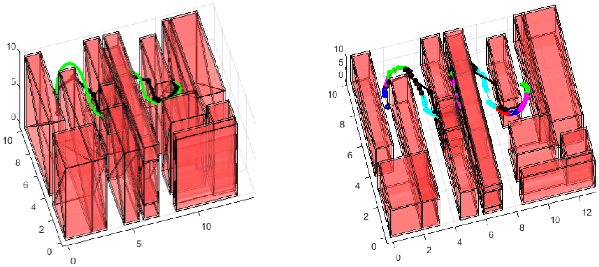
To assess the effectiveness of the Bézier curve-based back-end trajectory optimization method, this section establishes comparative experiments between ordinary polynomials and Bézier curves based on minimum snap optimization methods. Figure 18, Figure 19, Figure 20, Figure 21, Figure 22 and Figure 23 show trajectory comparisons planned by quadrotors in different scenarios. The green trajectory in the left figure is the minimum snap trajectory optimization method based on ordinary polynomials, and the right figure is the trajectory optimization method based on Bézier curves. Points of different colors in the figure correspond to the guiding vertices of every Bézier curve section. The actually planned trajectory also satisfies the properties of Bézier curves.
This section uses Bézier curves instead of traditional piecewise polynomials to represent trajectories. Only corresponding safety and kinodynamic feasibility constraints need to be imposed on control points, without needing to find extrema and iterative solving, and without additional constraints to ensure trajectories do not collide, effectively reducing algorithm complexity. For back-end trajectory optimization, we compared the cost function (i.e., the cumulative sum of snap squared (position’s 4th-order derivative)) and the time required to generate trajectories for both methods, as shown in Table 7. The proposed method has advantages in terms of time required to generate optimized trajectories, while also having smaller objective function values, reflecting that the generated trajectories are smoother with stable changes. Low Snap values can reduce control requirements on the system, ensure safety and stability, avoid possible energy waste, and improve overall energy utilization efficiency.
In trajectory optimization, Bézier curve representation demonstrates significant advantages over traditional piecewise polynomials. As shown in Table 7, our approach reduces snap integral by 40–55% across all scenarios, indicating substantially smoother trajectories. The computation time for optimization is reduced by 30–45%, attributed to the simplified constraint formulation enabled by the bounding envelope and velocity-hodograph characteristics of Bernstein-polynomial-based curves. The trajectories generated satisfy all kinodynamic constraints with maximum velocities and accelerations well within feasible bounds.
Visualization of the complete planning results (Figure 18, Figure 19, Figure 20, Figure 21, Figure 22 and Figure 23) reveals that our trajectories maintain smooth curvature throughout, with no abrupt direction changes or velocity discontinuities. The Bézier control points remain strictly within their respective safe corridors, confirming collision-free guarantees. Compared to ordinary polynomial trajectories, Bézier-based trajectories exhibit less oscillation near waypoints and more natural motion patterns suitable for quadrotor execution.

4.7. Motion Planning Method Comparison

To comprehensively evaluate the performance of the proposed safe-corridor-based UAV motion planning framework, this section compares it against Fast-Planner and EGO-Planner. Notably, EGO-Planner employs B-spline trajectory representation internally, so this comparison simultaneously covers B-spline-based trajectory planning methods. Kinodynamic planners target online replanning scenarios and operate under a fundamentally different problem formulation; they are therefore excluded from this offline optimization benchmark. Each method is executed ten times on randomly generated maps, and the cost function value, trajectory generation time, and success rate are recorded in Table 8.
The proposed framework is a hard-constraint optimization method that strictly enforces all constraints, guaranteeing that the final solution lies within the feasible domain. Fast-Planner and EGO-Planner are soft-constraint optimization methods that incorporate constraints as penalty terms in the objective function, permitting bounded constraint violations. Consequently, their success rates (95% and 96%, respectively) are lower than that of the proposed method (99%). When penalty coefficients are poorly tuned, soft-constraint methods may over-relax or over-tighten constraints, increasing the risk of infeasibility and local optima in multi-constraint problems.
The proposed method achieves the lowest average cost function value (973), indicating smoother trajectories with less aggressive state changes compared to Fast-Planner (1323) and EGO-Planner (1275). Trajectory generation time is comparable across all three methods. Although soft-constraint methods reduce computational overhead by converting constrained problems into unconstrained ones, the proposed method achieves competitive efficiency through the combined improvements of the JPS–Bresenham front-end path search, time allocation, and Bézier-based back-end optimization, which reduce iterative steps and complex computations without sacrificing constraint strictness.
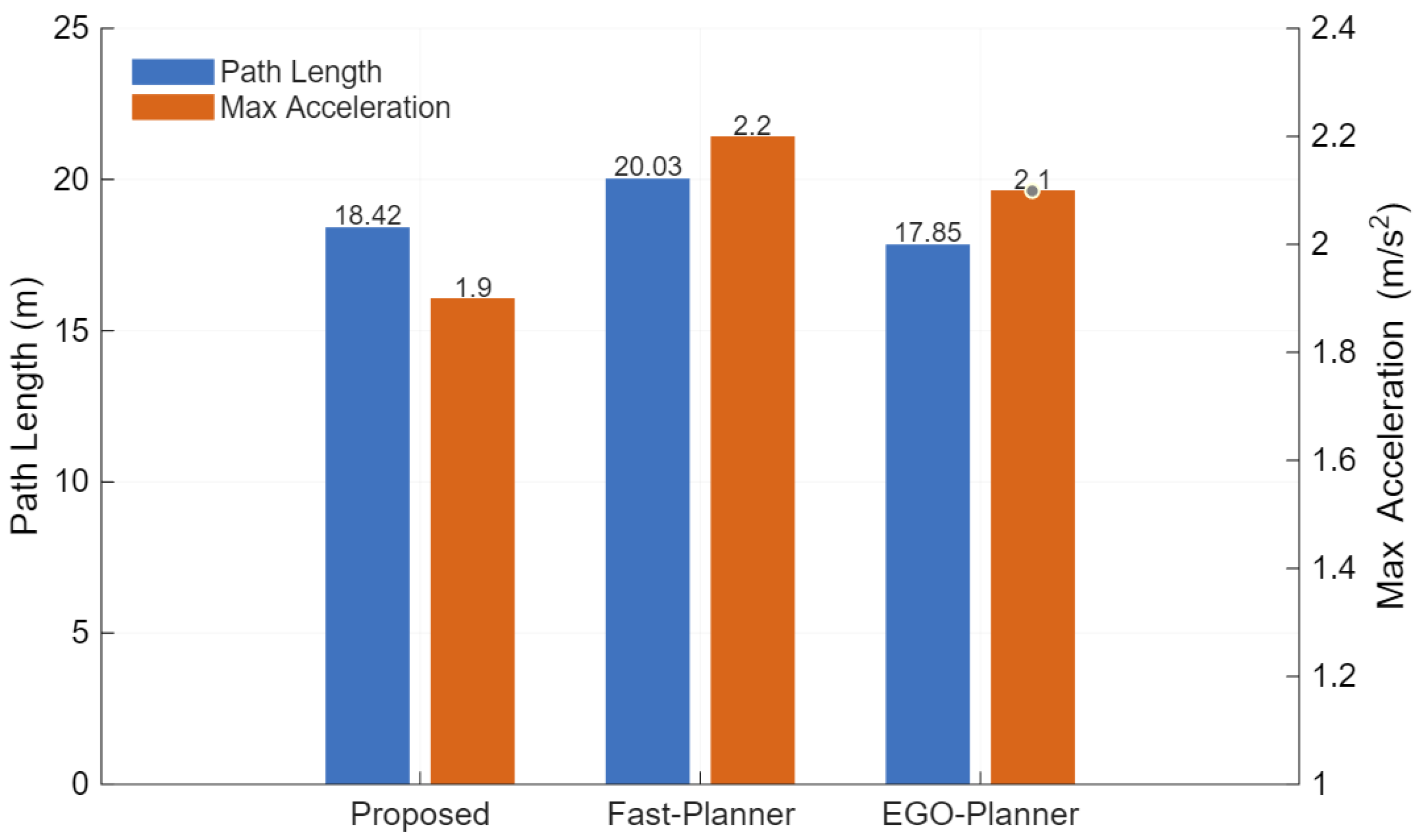
Figure 24 further illustrates the path length and maximum acceleration of the three methods. Path lengths are similar across methods, with EGO-Planner producing the shortest paths, the proposed method second, and Fast-Planner the longest. Critically, with the maximum acceleration constraint set to a max = 2 m / s 2 , both Fast-Planner and EGO-Planner generate trajectories whose peak acceleration exceeds this limit—a direct consequence of soft-constraint relaxation. In practice, a UAV may be unable to track such trajectories, posing a safety risk. The proposed method strictly enforces the dynamic feasibility constraint via hard constraints, ensuring all planned trajectories remain within the prescribed acceleration bound and are therefore directly deployable on physical platforms.

5. Conclusions

The present work investigates the quadrotor motion planning problem in cluttered environments, particularly for low-altitude economy and intelligent energy system applications such as infrastructure inspection and power line monitoring, where autonomous aerial vehicles require both computational efficiency and trajectory smoothness. We introduce a complete hierarchical planning framework to efficiently generate safe, smooth, and dynamically feasible trajectories. We apply a front-end JPS–Bresenham-based path search method on grid maps to identify optimal collision-free paths with reduced waypoints and superior computational efficiency compared to sampling-based approaches. Our JPS–Bresenham algorithm achieves 4–10% shorter paths with 40–83% faster computation compared to RRT* and PRM methods. Monte Carlo experiments validate robustness with 67.3% average waypoint reduction compared to JPS and superior scalability over A*. Comparisons with state-of-the-art planners show a 99% success rate with 22–27% lower cost function values than Fast-Planner and EGO-Planner. Safe flight corridors with overlapping regions are subsequently constructed to expand the solution space, followed by time allocation for each segment. Back-end Bézier curve-based trajectory optimization leverages the convex properties of these corridors through quadratic programming, achieving significant improvements in trajectory smoothness with 40–55% reduction in snap integral and 30–45% faster computation compared to ordinary polynomial methods. Experimental validation across multiple scenarios demonstrates near-zero position and velocity tracking errors. For future work, we plan to extend the proposed framework to dynamic environments by incorporating temporal safety constraints for moving obstacle avoidance, and explore multi-drone cooperative motion planning with distributed corridor construction.
Although the proposed algorithm has been thoroughly validated through simulation experiments, real-world flight validation remains an important direction for future work. The current study is exploratory in nature, focusing on algorithmic design and performance benchmarking within controlled simulation environments. Deploying the algorithm on a physical platform would require substantial hardware infrastructure, including high-precision localization systems and reliable onboard computing units, which demands considerable engineering effort beyond the scope of this initial investigation. Moreover, systematically reproducing extreme real-world conditions, such as dynamic obstacle fields and GPS-denied environments, presents significant practical challenges. Simulation-based evaluation therefore provides a rigorous and scalable basis for assessing algorithmic performance at this stage. In future work, we plan to deploy the proposed algorithm on a physical drone platform and conduct field experiments in representative logistics scenarios to further verify its practical applicability and robustness. Additionally, we will evaluate the computational performance on resource-constrained onboard hardware to validate the method’s feasibility for time-critical applications.

Author Contributions

Conceptualization, X.M. and N.D.; methodology, X.M. and W.L.; software, X.M. and S.L.; validation, X.M., W.L. and S.L.; formal analysis, X.M.; investigation, X.M. and W.L.; resources, N.D.; data curation, X.M. and S.L.; writing—original draft preparation, X.M.; writing—review and editing, W.L., N.D. and S.L.; visualization, X.M.; supervision, N.D.; project administration, N.D.; funding acquisition, N.D. All authors have read and agreed to the published version of the manuscript.

Funding

This research was funded by the National Natural Science Foundation of China, grant number 62273253, and the Key Program of the Natural Science Foundation of Tianjin, China, grant number 22JCZDJC00330.

Data Availability Statement

The original contributions presented in this study are included in the article. Further inquiries can be directed to the corresponding author.

Conflicts of Interest

Author Xiaoming Mai was employed by the company The Intelligent Operation and Inspection Division of China Southern Power Grid Technology Co., Ltd., Guangzhou 510170, China. The remaining authors declare that the research was conducted in the absence of any commercial or financial relationships that could be construed as a potential conflict of interest.

References

  1. Rejeb, A.; Rejeb, K.; Simske, S.J.; Treiblmaier, H. Drones for supply chain management and logistics: A review and research agenda. Int. J. Logist. Res. Appl. 2023, 26, 708–731. [Google Scholar] [CrossRef] [Scilit]
  2. Sah, B.; Gupta, R.; Bani-Hani, D. Analysis of barriers to implement drone logistics. Int. J. Logist. Res. Appl. 2021, 24, 531–550. [Google Scholar] [CrossRef] [Scilit]
  3. Pachayappan, M.; Sundarakani, B. Drone delivery logistics model for on-demand hyperlocal market. Int. J. Logist. Res. Appl. 2023, 26, 1728–1760. [Google Scholar] [CrossRef] [Scilit]
  4. Li, Y.; Liu, M.; Jiang, D. Application of unmanned aerial vehicles in logistics: A literature review. Sustainability 2022, 14, 14473. [Google Scholar] [CrossRef] [Scilit]
  5. Zrelli, I.; Rejeb, A.; Abusulaiman, R.; AlSahafi, R.; Rejeb, K.; Iranmanesh, M. Drone applications in logistics and supply chain management: A systematic review using latent Dirichlet allocation. Arab. J. Sci. Eng. 2024, 49, 12411–12430. [Google Scholar] [CrossRef] [Scilit]
  6. Jazairy, A.; Persson, E.; Brho, M.; von Haartman, R.; Hilletofth, P. Drones in last-mile delivery: A systematic literature review from a logistics management perspective. Int. J. Logist. Manag. 2024, 36, 1–62. [Google Scholar] [CrossRef] [Scilit]
  7. Wu, K.; Lan, J.; Lu, S.; Wu, C.; Liu, B.; Lu, Z. Integrative path planning for multi-rotor logistics UAVs considering UAV dynamics, energy efficiency, and obstacle avoidance. Drones 2025, 9, 93. [Google Scholar] [CrossRef] [Scilit]
  8. Cheng, Q.; Zhang, Z.; Du, Y.; Li, Y. Research on particle swarm optimization-based UAV path planning technology in urban airspace. Drones 2024, 8, 701. [Google Scholar] [CrossRef] [Scilit]
  9. Mellinger, D.; Kumar, V. Minimum snap trajectory generation and control for quadrotors. In Proceedings of the 2011 IEEE International Conference on Robotics and Automation, Shanghai, China, 9–13 May 2011; pp. 2520–2525. [Google Scholar] [CrossRef] [Scilit]
  10. Burke, D.; Chapman, A.; Shames, I. Generating minimum-snap quadrotor trajectories really fast. In Proceedings of the 2020 IEEE/RSJ International Conference on Intelligent Robots and Systems (IROS), Las Vegas, NV, USA, 24 October–24 January 2021; pp. 1487–1492. [Google Scholar] [CrossRef] [Scilit]
  11. Manzoni, M.; Rubinacci, R.; Invernizzi, D. Efficient motion primitives-based trajectory planning for UAVs in the presence of obstacles. Drones 2024, 8, 256. [Google Scholar] [CrossRef] [Scilit]
  12. Zhou, B.; Gao, F.; Wang, L.; Liu, C.; Shen, S. Robust and efficient quadrotor trajectory generation for fast autonomous flight. IEEE Robot. Autom. Lett. 2019, 4, 3529–3536. [Google Scholar] [CrossRef] [Scilit]
  13. Gao, F.; Wu, W.; Lin, Y.; Shen, S. Online safe trajectory generation for quadrotors using fast marching method and Bernstein basis polynomial. In Proceedings of the 2018 IEEE International Conference on Robotics and Automation (ICRA), Brisbane, QLD, Australia, 21–25 May 2018; pp. 344–351. [Google Scholar] [CrossRef] [Scilit]
  14. Kumar, P.; Pal, K.; Govil, M.C. Comprehensive review of path planning techniques for unmanned aerial vehicles (UAVs). ACM Comput. Surv. 2025, 58, 1–44. [Google Scholar] [CrossRef] [Scilit]
  15. Wang, B.; Zhang, Y.; Zhang, W. Integrated path planning and trajectory tracking control for quadrotor UAVs with obstacle avoidance in the presence of environmental and systematic uncertainties: Theory and experiment. Aerosp. Sci. Technol. 2022, 120, 107277. [Google Scholar] [CrossRef] [Scilit]
  16. Zhai, Z.; Gao, Y.; Ni, W.; Yuan, X.; Wang, X. Trajectory Design for UAV-Assisted Logistics Collection in Low-Altitude Economy. arXiv 2025, arXiv:2511.07178. [Google Scholar] [CrossRef] [Scilit]
  17. Zou, F.; Li, J.; Niu, Y. Motion planning for agile fixed-wing UAVs in complex low-altitude environments. Robotica 2025, 43, 1640–1659. [Google Scholar] [CrossRef] [Scilit]
  18. Saunders, J.; Saeedi, S.; Li, W. Autonomous aerial robotics for package delivery: A technical review. J. Field Robot. 2024, 41, 3–49. [Google Scholar] [CrossRef] [Scilit]
  19. Quan, L.; Han, L.; Zhou, B.; Shen, S.; Gao, F. Survey of UAV motion planning. IET Cyber-Syst. Robot. 2020, 2, 14–21. [Google Scholar] [CrossRef] [Scilit]
  20. Allaire, F.C.J.; Labonté, G.; Tarbouchi, M.; Roberge, V. Recent advances in unmanned aerial vehicles real-time trajectory planning. J. Unmanned Veh. Syst. 2019, 7, 259–295. [Google Scholar] [CrossRef] [Scilit]
  21. Liu, S.; Watterson, M.; Mohta, K.; Sun, K.; Bhattacharya, S.; Taylor, C.J.; Kumar, V. Planning dynamically feasible trajectories for quadrotors using safe flight corridors in 3-D complex environments. IEEE Robot. Autom. Lett. 2017, 2, 1688–1695. [Google Scholar] [CrossRef] [Scilit]
  22. Park, J.; Kim, H.J. Online trajectory planning for multiple quadrotors in dynamic environments using relative safe flight corridor. IEEE Robot. Autom. Lett. 2020, 6, 659–666. [Google Scholar] [CrossRef] [Scilit]
  23. Sun, J.; Xu, G.; Wang, Z.; Long, T.; Sun, J. Safe flight corridor constrained sequential convex programming for efficient trajectory generation of fixed-wing UAVs. Chin. J. Aeronaut. 2025, 38, 103174. [Google Scholar] [CrossRef] [Scilit]
  24. Miao, H.; Long, T.; Sun, J.; Li, J.; Wang, S.; Zhou, Z. Hierarchical Trajectory Sequential Convex Programming Method for UAV Based on Safe Flight Corridors. In Proceedings of the International Conference on Guidance, Navigation and Control, Changsha, China, 9–11 August 2024; pp. 306–316. [Google Scholar]
  25. Ren, Y.; Zhu, F.; Liu, W.; Wang, Z.; Lin, Y.; Gao, F.; Zhang, F. Bubble planner: Planning high-speed smooth quadrotor trajectories using receding corridors. In Proceedings of the 2022 IEEE/RSJ International Conference on Intelligent Robots and Systems (IROS), Kyoto, Japan, 23–27 October 2022; pp. 6332–6339. [Google Scholar] [CrossRef] [Scilit]
  26. Ren, Y.; Zhu, F.; Lu, G.; Cai, Y.; Yin, L.; Kong, F.; Lin, J.; Chen, N.; Zhang, F. Safety-assured high-speed navigation for MAVs. Sci. Robot. 2025, 10, eado6187. [Google Scholar] [CrossRef] [Scilit]
  27. Satai, H.A.; Zahra, M.M.A.; Rasool, Z.I.; Abd-Ali, R.S.; Pruncu, C.I. Bézier curves-based optimal trajectory design for multirotor UAVs with any-angle pathfinding algorithms. Sensors 2021, 21, 2460. [Google Scholar] [CrossRef] [Scilit] [PubMed]
  28. Tang, L.; Wang, H.; Li, P.; Wang, Y. Real-time trajectory generation for quadrotors using B-spline based non-uniform kinodynamic search. In Proceedings of the 2019 IEEE International Conference on Robotics and Biomimetics (ROBIO), Dali, China, 6–8 December 2019; pp. 1133–1138. [Google Scholar] [CrossRef] [Scilit]
  29. Wang, L.; Guo, Y. Speed adaptive robot trajectory generation based on derivative property of B-spline curve. IEEE Robot. Autom. Lett. 2023, 8, 1905–1911. [Google Scholar] [CrossRef] [Scilit]
  30. Kheireddine, C.; Yassine, A.; Fawzi, S.; Khalil, M. A robust synergetic controller for quadrotor obstacle avoidance using Bezier curve versus B-spline trajectory generation. Intell. Serv. Robot. 2022, 15, 143–152. [Google Scholar] [CrossRef] [Scilit]
  31. Liu, J.; Luo, W.; Zhang, G.; Li, R. Unmanned aerial vehicle path planning in complex dynamic environments based on deep reinforcement learning. Machines 2025, 13, 162. [Google Scholar] [CrossRef] [Scilit]
  32. Pan, Y.; Cheng, C.-A.; Saigol, K.; Lee, K.; Yan, X.; Theodorou, E.A.; Boots, B. Imitation learning for agile autonomous driving. Int. J. Robot. Res. 2020, 39, 286–302. [Google Scholar] [CrossRef] [Scilit]
  33. Holmsen, A.F. Helly type problems in convexity spaces. arXiv 2024, arXiv:2408.05871. [Google Scholar] [CrossRef] [Scilit]
  34. Jiang, M.; Li, Y.; Zhang, Q.; Qin, J. Joint position and time allocation optimization of UAV enabled time allocation optimization networks. IEEE Trans. Commun. 2019, 67, 3806–3816. [Google Scholar] [CrossRef] [Scilit]
  35. Karakılıç, İ.; Karakılıç, S.; Budakçı, G.; Özger, F. Bézier curves and surfaces with the blending (α, λ, s)-Bernstein basis. Symmetry 2025, 17, 219. [Google Scholar] [CrossRef] [Scilit]
  36. Harabor, D.; Grastien, A. The JPS pathfinding system. In Proceedings of the International Symposium on Combinatorial Search, Niagara Falls, ON, Canada, 19–21 July 2012; Volume 3, pp. 207–208. [Google Scholar] [CrossRef] [Scilit]
  37. Wang, Z.; Zhou, X.; Xu, C.; Gao, F. Geometrically constrained trajectory optimization for multicopters. IEEE Trans. Robot. 2022, 38, 3259–3278. [Google Scholar] [CrossRef] [Scilit]
  38. Zhou, B.; Pan, J.; Gao, F.; Shen, S. Raptor: Robust and perception-aware trajectory replanning for quadrotor fast flight. IEEE Trans. Robot. 2021, 37, 1992–2009. [Google Scholar] [CrossRef] [Scilit]
  39. Velikzhanin, A.; Skarga-Bandurova, I. A Bresenham-based global path planning algorithm on grid maps. In Proceedings of the 2023 13th International Conference on Dependable Systems, Services and Technologies (DESSERT), Athens, Greece, 13–15 October 2023; pp. 1–8. [Google Scholar] [CrossRef] [Scilit]
  40. Wang, Q.; Wang, Z.; Wang, M.; Ji, J.; Han, Z.; Wu, T.; Jin, R.; Gao, Y.; Xu, C.; Gao, F. Fast iterative region inflation for computing large 2-D/3-D convex regions of obstacle-free space. IEEE Trans. Robot. 2025, 41, 3223–3243. [Google Scholar] [CrossRef] [Scilit]
  41. Alqudsi, Y.; Makaraci, M.; Kassem, A.; El-Bayoumi, G. A numerically-stable trajectory generation and optimization algorithm for autonomous quadrotor UAVs. Robot. Auton. Syst. 2023, 170, 104532. [Google Scholar] [CrossRef] [Scilit]
  42. Zhou, X.; Wang, Z.; Ye, H.; Xu, C.; Gao, F. Ego-planner: An ESDF-free gradient-based local planner for quadrotors. IEEE Robot. Autom. Lett. 2020, 6, 478–485. [Google Scholar] [CrossRef] [Scilit]
  43. Du, B.; Chen, J.; Sun, D.; Manyam, S.G.; Casbeer, D.W. UAV trajectory planning with probabilistic geo-fence via iterative chance-constrained optimization. IEEE Trans. Intell. Transp. Syst. 2021, 23, 5859–5870. [Google Scholar] [CrossRef] [Scilit]
  44. Gong, H.; Tan, X.; Wu, Q.; Li, J.; Chu, Y.; Jiang, A.; Han, H.; Zhang, K. Bidirectional jump point search path-planning algorithm based on electricity-guided navigation behavior of electric eels and map preprocessing. Biomimetics 2023, 8, 387. [Google Scholar] [CrossRef] [Scilit]
  45. Ganesan, S.; Ramalingam, B.; Mohan, R.E. A hybrid sampling-based RRT* path planning algorithm for autonomous mobile robot navigation. Expert Syst. Appl. 2024, 258, 125206. [Google Scholar] [CrossRef] [Scilit]
  46. Hüppi, M.; Bartolomei, L.; Mascaro, R.; Chli, M. T-PRM: Temporal probabilistic roadmap for path planning in dynamic environments. In Proceedings of the 2022 IEEE/RSJ International Conference on Intelligent Robots and Systems (IROS), Kyoto, Japan, 23–27 October 2022; pp. 10320–10327. [Google Scholar] [CrossRef] [Scilit]
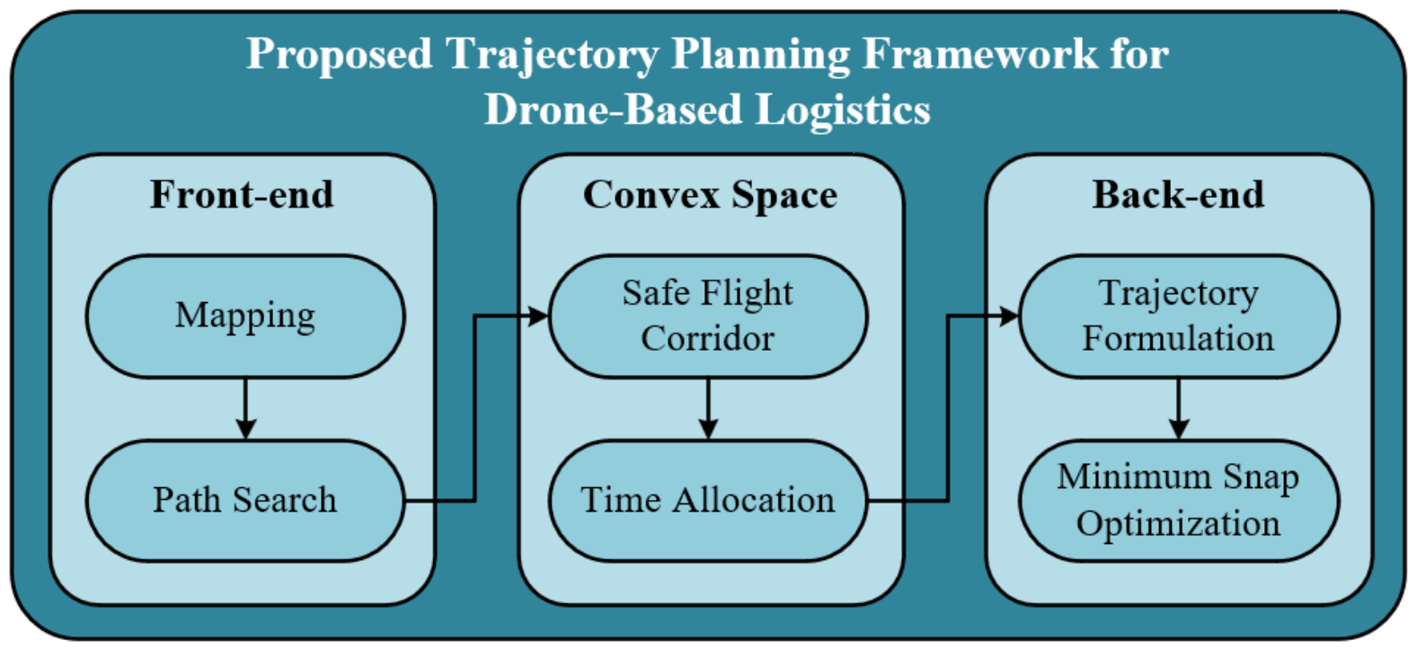
Figure 1. Proposed hierarchical trajectory planning framework. Three modules: (1) front-end: JPS–Bresenham path search (input: map, start, goal; output: waypoints); (2) middle: safe corridor construction via ellipsoid fitting and convex polyhedra with time allocation (output: corridors and times); (3) back-end: Bézier curve optimization transforming non-convex to linear constraints (output: smooth trajectory). Arrows show data flow.
Drones 10 00323 g001
Figure 2. Neighboring nodes without obstacles.
Drones 10 00323 g002
Figure 3. Forced neighbors with obstacles.
Drones 10 00323 g003
Figure 4. Simple environment.
Drones 10 00323 g004
Figure 5. Medium-complexity environment.
Drones 10 00323 g005
Figure 6. Complex environment.
Drones 10 00323 g006
Figure 7. Bresenham algorithm diagram.
Drones 10 00323 g007
Figure 8. Trapezoidal velocity profile for time allocation. The three phases correspond to Equations (9)–(11): acceleration phase (0 to T a ) with quadratic displacement, constant velocity phase ( T a to T T a ) with linear displacement, and deceleration phase ( T T a to T) with quadratic displacement. The velocity reaches maximum v max at time T a = v max / a max and maintains this value until deceleration begins.
Drones 10 00323 g008
Figure 9. Map1 path search result comparison.
Drones 10 00323 g009
Figure 10. Map2 path search results comparison.
Drones 10 00323 g010
Figure 11. Map3 path search result comparison.
Drones 10 00323 g011
Figure 12. Map4 path search result comparison.
Drones 10 00323 g012
Figure 13. Map5 path search result comparison.
Drones 10 00323 g013
Figure 14. Map6 path search result comparison.
Drones 10 00323 g014
Figure 15. Simple environment ellipsoid fitting results.
Drones 10 00323 g015
Figure 16. Medium-complexity environment ellipsoid fitting results.
Drones 10 00323 g016
Figure 17. Complex environment ellipsoid fitting results.
Drones 10 00323 g017
Figure 18. Map1 trajectory optimization result comparison.
Drones 10 00323 g018
Figure 19. Map2 trajectory optimization result comparison.
Drones 10 00323 g019
Figure 20. Map3 trajectory optimization result comparison.
Drones 10 00323 g020
Figure 21. Map4 trajectory optimization result comparison.
Drones 10 00323 g021
Figure 22. Map5 trajectory optimization result comparison.
Drones 10 00323 g022
Figure 23. Map6 trajectory optimization result comparison.
Drones 10 00323 g023
Figure 24. Path length and maximum acceleration comparison among three motion planning methods.
Drones 10 00323 g024
Table 1. Simple environment obstacle parameters.
ObstacleMap1Map2
Lower-LeftUpper-RightLower-LeftUpper-Right
1(1, 0.5, 0.1)(2, 0.7, 3)(2.25, 0, 0)(2.65, 1.9, 3.4)
2(0, 1.5, 0)(1, 1.7, 3)(0.05, 1.1, 0)(0.45, 3, 3.4)
3(2, 1.5, 0.1)(3, 1.7, 3)(4.5, 1.1, 0)(4.9, 3, 3.4)
Table 2. Medium-complexity environment obstacle parameters.
ObstacleMap3Map4
Lower-LeftUpper-RightLower-LeftUpper-Right
1(0, 2, 0)(10, 2.5, 1.5)(3.1, 0, 2.1)(3.9, 5, 6)
2(0, 2, 4.5)(10, 2.5, 6)(9.1, 0, 2.1)(9.9, 5, 6)
3(0, 2, 1.5)(3, 2.5, 4.5)(15.1, 0, 2.1)(15.9, 5, 6)
4(7, 2, 1.5)(10, 2.5, 4.5)(0.1, 0, 0)(0.9, 5, 3.9)
5(3, 0, 2.4)(7, 0.5, 4.5)(6.1, 0, 0)(6.9, 5, 3.9)
6(0, 15, 0)(0, 10, 20)(12.1, 0, 0)(12.9, 5, 3.9)
7(0, 15, 1)(1, 10, 16)(18.1, 0, 0)(18.9, 5, 3.9)
8(0, 18, 4.5)(10, 19, 6)
Table 3. Complex environment obstacle parameters.
ObstacleMap5Map6
Lower-LeftUpper-RightLower-LeftUpper-Right
1(0, −5, 0)(10, 20, 6)(0, 4, 0)(1, 10, 10)
2(0, −2, 3)(10, −1.5, 6)(0, 0, 0)(3, 3, 10)
3(0, −2, 1.5)(3, −1.5, 3)(2, 0, 0)(3, 8, 10)
4(6, −2, 1.5)(10, −1.5, 3)(4.5, 6, 0)(5.5, 10, 10)
5(0, 2, 0)(10, 2.5, 1.5)(4.5, 4, 0)(5.5, 6, 3.5)
6(0, 2, 4.5)(10, 2.5, 6)(4.5, 4, 6.5)(5.5, 6, 10)
7(0, 7, 0)(10, 7.5, 0.5)(4.5, 0, 0)(5.5, 4, 10)
8(0, 7, 2)(10, 7.5, 5.5)(6, 0, 0)(7, 10, 2)
9(0, 11, 0)(10, 11.5, 2.5)(6, 8.5, 2)(7, 10, 8)
10(0, 11, 4)(10, 11.5, 5.5)(6, 4, 2)(7, 7.5, 8)
11(0, −2, 0)(0, 10, −1.5)(6, 0, 2)(7, 2, 8)
12(0, −2, 3)(10, −1.5, 5.5)(6, 0, 8)(7, 10, 10)
13(0, 2, 1.5)(3, 2.5, 4.5)(8.5, 5, 0)(9.5, 9, 10)
14(7, 2, 1.5)(10, 2.5, 4.5)(8.5, 1.5, 0)(11, 3.5, 10)
15(3, 0, 2.4)(7, 0.5, 4.5)(8.5, 0, 0)(13, 0.5, 10)
16(0, 15, 0)(10, 20, 1)(10.5, 3.5, 0)(11, 10, 10)
17(0, 15, 1)(10, 16, 3.5)(11, 3, 0)(13, 10, 10)
18(0, 18, 4.5)(10, 19, 6)(11.5, 0.5, 0)(13, 2, 10)
Table 4. Performance comparison of different algorithms for path planning.
MapAlgorithmPath LengthWaypointsTime (s)
Map1JPS [44]3.7276130.13
RRT* [45]5.509864.82
PRM [46]5.236573.37
JPS–Bresenham3.485980.15
Map2JPS14.6572260.21
RRT*14.945295.24
PRM16.933864.56
JPS–Bresenham14.282580.24
Map3JPS23.0685250.64
RRT*23.398884.89
PRM27.258365.02
JPS–Bresenham22.677760.28
Map4JPS27.1576470.82
RRT*28.2183137.20
PRM32.1264145.59
JPS–Bresenham25.8701130.91
Map5JPS24.4271320.61
RRT*24.879194.21
PRM25.831694.55
JPS–Bresenham23.3693140.68
Map6JPS19.0359390.37
RRT*18.813695.68
PRM19.135094.86
JPS–Bresenham18.4513180.45
Table 5. Monte Carlo statistical results (mean of 50 trials).
ConfigAlgorithmPath Length (m)WaypointsTime (s)
Small–LowA*9.0549.30.270
JPS7.8210.40.046
JPS–Bresenham7.393.40.046
Small–HighA*7.6042.00.150
JPS7.2715.90.037
JPS–Bresenham6.947.10.036
Medium–LowA*18.2795.46.001
JPS17.3921.40.303
JPS–Bresenham16.648.10.303
Medium–HighA*14.7677.82.222
JPS13.3723.90.067
JPS–Bresenham12.588.60.066
Large–LowA*35.21180.1113.939
JPS34.3542.82.117
JPS–Bresenham31.9610.72.113
Large–HighA*31.39161.073.639
JPS32.2253.00.383
JPS–Bresenham30.8716.90.380
Table 6. Ellipsoid fitting computation time (seconds).
MapMap1Map2Map3Map4Map5Map6
Time0.0410.0560.0990.1240.1540.183
Table 7. Trajectory optimization performance comparison.
MapIntegral of Snap SquaredTime (s)
Ordinary PolynomialBézier CurveOrdinary PolynomialBézier Curve
Map115768420.0550.032
Map27965820.0730.048
Map3254614700.0860.063
Map4313118560.1050.087
Map5453721050.1580.103
Map6568725740.2560.141
Table 8. Motion planning method comparison.
Method Cost FunctionTime (s)Success Rate
Proposed
(Safe Corridor)
Max10240.4499%
Avg9730.37
Min9580.34
Fast-Planner [12]Max15370.4695%
Avg13230.41
Min12480.35
EGO-Planner [42]Max14890.4396%
Avg12750.37
Min10940.32
Disclaimer/Publisher’s Note: The statements, opinions and data contained in all publications are solely those of the individual author(s) and contributor(s) and not of MDPI and/or the editor(s). MDPI and/or the editor(s) disclaim responsibility for any injury to people or property resulting from any ideas, methods, instructions or products referred to in the content.